


I. Introduction
Although satellite-altimeter radars were initially devised for operating over the ocean, potentialities of this instrument in the study of continental ice sheets were demonstrated very early (Reference Brooks, Campbell, Ramseier, Stanley and ZwallyBrooks and others, 1978; Reference Zwally, Bindschadler, Brenner, Martin and ThomasZwally and others, 1983).
Estimation of the mass balance of polar ice sheets or modeling of ice-sheet flow require an accuracy of the order of 10 cm in the measurement of ice-surface elevation. Reference Remy, Mazzega, Houry, Brossier and MinsterRemy and others (1989) have shown that the precision of the topography derived from a satellite-altimeter radar over the Antarctic ice sheet may be at the present time around 0.5–3 m and also shown how the associated error maps can be derived, on the condition that the initial measurement-error budget is known.
In addition to the well-known limits of altimeter radars over open water, other errors are specific to continental ice sheets, such as the surface-slope error (Reference Brenner, Bindschadler, Thomas and ZwallyBrenner and others, 1983) or the inadequate tracking algorithms. Indeed, in contrast to the ocean, ice sheets present surface slopes of the order of 1°. In addition, radar-echo wave forms are affected by large-scale undulations (Reference Martin, Zwally, Brenner and BindschadlerMartin and others, 1983) and by medium-scale features (snow dunes or sastrugi), so that the echo modeling is not as simple as for the ocean. Moreover, Reference Ridley and PartingtonRidley and Partington (1988) and Reference Partington, Ridley, Rapley and ZwallyPartington and others (1989) have suggested that the altimeter return is also influenced by volume-scattering. Because of this effect, the estimated elevation measured by the radar altimeter is lower than the actual surface. Furthermore, as volume-scattering depends on snow-grain characteristics, it may not be constant with time. This may seriously affect the potential of satellite altimeters to monitor ice-sheet surface elevations.
As many parameters affect the radar wave forms (Reference RapleyRapley and others, 1983; Reference Ridley and PartingtonRidley and Partington, 1988; Reference Guzkowska, Rapley, Ridley, Cudlip, Birkett and ScottGuzkowska and others, 1990), it is difficult to analyse the relative importance of their effects both because of the insufficient understanding of the physics of the scattering and because of the lack of values for these parameters.
Up to now, most altimetric wave-form simulators over ice sheets did not take into account volume-scattering, while modelling the latter has been achieved analytically (Reference Partington and RapleyPartington and Rapley, 1986; Reference Ridley and PartingtonRidley and Partington, 1988; Reference Partington, Ridley, Rapley and ZwallyPartington and others, 1989). Here, we attempt to model volume-and surface-scattering simultaneously by adapting an altimeter wave-form simulator developed for a planetary radar (Reference ThouvenotThouvenot, 1990). Because the effect of the different snow parameters on the altimetric-height precision depends on the applied re-tracking technique, the existing techniques will be compared to estimate possible biases on the surface-height measurement due to volume-scattering. In this paper, we will focus the study on an area of Antarctica where the altitude is greater than 1000 m, because near the coast, other errors may lead to poor accuracy. Thus, the surface characteristics (undulations) or volume characteristics (temperature and snow conditions) are selected as appropriate for such high altitudes.
The first section of the paper deals with the simulation of the surface effect, using an ice-sheet surface model. The paper continues with the simulation of the volume effect, and finally with its impact on the accuracy of the altimetric measurement.
II. Principles of Wave-Form Simulation
The altimeter wave-form simulator is based on two basic elements: the radar and the studied body, in this case the ice sheets.
The altimeter emits radar pulses at a pulse-rate frequency (PRF) of 1000–4000 Hz and records the reflected energy after its interaction with the illuminated area. Only a sample of each pulse echo is recorded in the radar-receiving window. One can consider the returned wave form of the radar pulse as the cumulative histogram of the energy returned from each illuminated surface point, sampled by a series of gates in the receiving window. For the Seasat altimeter, each of the 60 gates measured the energy return during a time, τ, of 3.125 ns. The instantaneous power (without thermal noise) received at time t from an illuminated point has been given by Reference MacArthurMacArthur (1978) as:

where t’ is the arrival time of each illuminated point, d is the distance between the satellite and the aimed point, r is a 3.125 ns gate, σ0 is the back-scatter coefficient, dS is a physical surface element, G is the real antenna gain, Β is the band width, T is the pulse width (3.2µs), L is the propagation losses, λ is the radar wavelength and Pe is its emitted power; c is the speed of light. The contribution of each physical surface element is therefore characterized by the time t of arrival, which depends on its position in the illuminated area and on the surface topography, and by its back-scatter coefficient σ0
The wave form of the radar echo from a flat surface can be separated into two parts. Its leading edge is caused by the initial interaction of the pulse with an expanding quasi-circular area, the maximum width of which is affected by the radar-pulse length and the medium-scale features such as sastrugi. At its maximum width, this area is known as the pulse-limited footprint. After this initial stage, the illuminated surface becomes an annulus of progressively increasing radius and approximately constant surface area. The reflected energy from this annulus is attenuated by the antenna pattern and forms the trailing edge of the wave form.
Considering the availability of Seasat data over Antarctica and the desire to make comparative tests, we modeled the altimeter simulator on the description of the Seasat altimeter (Reference MacArthurMacArthur, 1978). This altimeter operated at a frequency of 13.6 GHz (λ = 2.3 cm), where the echo is mostly sensitive to surface features. Indeed, at this frequency, the volume echo, due to back-scatter of the radar signal from below the snow surface, is not dominant (see below). The transmitted pulse has a band width Β = 320 MHz. The antenna is a 1 m parabolic dish. Over a flat surface, the diameter of the beam-limited illuminated surface depends on the 3 dB two-way antenna beam width defined in degrees as:
where λ is in cm and D, the parabolic dish diameter, is in meters.
The software simulator generates return wave forms for different off-nadir pointing angles (Fig. 1) from different simulated surfaces. One can schematically describe the software in three successive parts: first, the spacecraft configuration includes effects of the elevation and geographic location of the satellite, and of the off-nadir pointing angle. Secondly, the pulse-limited footprint is determined according to its location in the beam-limited footprint, taking account of surface slope and roughness. The width of the acquisition window, within which the return energy is recorded, has been set at 40 m, as a compromise between computed execution time and compatibility with surface roughness. This leads to considering 6 × 10⁵ points in the illuminated area. Thirdly, the different characteristics of the surface-or volume-scattering are then easily taken into account according to their statistical distribution, using a Monte Carlo technique.

Fig. 1. Schematic representation of the simulator geometry, with the nadir N, the off-pointing angle β giving P, the point of sight. δ is the 3 dB beam width. The elevation h for each modeled sastruga is taken at random. I, the incidence angle involved in the back-scatter coefficient, and α, the angle involved in the radar beam and the corresponding antenna gain, are computed for each of them.
Finally, the temporal evolution of the echo is calculated by summing the responses of all points from the illuminated surface, at their corresponding arrival times.
III. Modeling Surface Features
The topography of ice sheets, and more especially of Antarctica, can be described by four main kinds of relief: two on a large scale—the near-parabolic profile and undulations — both related to the ice flow above the bedrock (Reference McIntyre and DrewryMcIntyre and Drewry, 1984), and two on medium to small scales — sastrugi and micro-roughness — created by winds (Reference KobayashiKobayashi, 1979). The smaller-scale features, micro-roughness, affect the back-scatter coefficient. The other scales affect the back-scatter coefficient and/or the arrival time.
Micro-roughness is taken into account in either one of two models of back-scattering, one with a Gaussian distribution of slopes and the other with an exponential distribution (Reference Fung and EomFung and Eom, 1983). As an example, the former is described by:

where s2 is the r.m.s. surface slope, I is the incidence angle (see Fig. 1 ) and R is the Fresnel coefficient taken at the vertical and given by:

where ε, the dielectric constant, is linked to the snow density (Reference Tiuri, Sihvola, Nyfors and HallikainenTiuri and others, 1984). This back-scatter model is adapted from that for the oceanic surface. No in-situ data are available to verify its validity. However, from this model, the echo decreases rapidly from about 5 dB at the vertical to −5 dB at 20° incidence, as is observed by the Seasat scatterometer data (Reference Ledroit, Remy and MinsterLedroit and others, 1993), which operated at the same frequency as the altimeter. With this back-scatter model, the contribution of each iluminated point will only depend on the angle between the normal vector to its surface element and the incident-beam direction (Fig. 1). The observed σ0 values from the Seasat altimeter vary from 1 to 10 dB, with a mean value of 3 (Reference Remy and MinsterRemy and others, 1990). a will always be set to 0.07 leading to σ0 = 1 dB, which is thus the minimum value.
Sastrugi are from centimeters to about 1 m in height and up to 10 m in wavelength (Reference McIntyre and DrewryMcIntyre and Drewry, 1984). These features are elongated in the katabatic upwind direction and are disymmetric with one side steeper than the other. In the simulation, only energy reflected from the gently sloping side is taken into account, considering that the return power from the other side is insignificant in comparison. Thus, sastrugi are modeled by three points of elevation taken randomly for each illuminated point (Fig. 1).
Large-scale undulations are dome-shaped with heights of the order of meters to tens of meters and wavelengths of kilometers to tens of kilometers (Fig. 2b). They affect the radar wave forms because the corresponding curvature of the surface varies on the same scale as the illuminated area (Reference Martin, Zwally, Brenner and BindschadlerMartin and others, 1983). In the altimeter simulator, the elevation connected to this modeled relief is estimated at each point in the illuminated surface by a two-dimensional sine function.
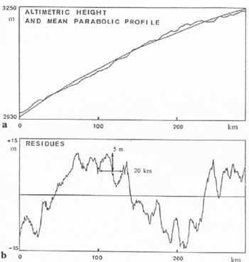
Fig. 2. Seasat altimetric profile above the Antarctic ice sheet fitted by a parabolic function (a) and its residual height showing undulations (b). From Reference Remy, Mazzega, Houry, Brossier and MinsterRemy and others (1989).
As shown in Figure 2a, a near-parabolic surface fits the large-scale ice-sheet topography over a few hundred kilometers. In an altimetric measurement, the diameter of the beam-limited footprint is 20 km to 30 km, and the pulse-limited footprint is considerably smaller, so that the parabolic relief can be approximated as a plane. In the software, we modeled this as equivalent to an off-nadir pointing angle. Indeed, the same wave form can be created by two different configurations (see Fig. 3) by an off-nadir pointing angle or by a surface slope. Note that the altimetric height relates to the distance of the nearest point from the satellite, which is shifted from the nadir N. This effect is called the slope-induced error and can be corrected at a later stage, during data processing (Reference Brenner, Bindschadler, Thomas and ZwallyBrenner and others, 1983; Reference Remy, Mazzega, Houry, Brossier and MinsterRemy and others, 1989).
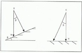
Fig. 3. Geometry for the large-scale slope effect. The large-scale topographic features (a) are taken into account as an off-nadir pointing angle (β in Fig. 1) of the same value (b).
IV. Tests with Tracking Algorithms over Simulated Surfaces
Figure 4a–c shows examples of simulated wave forms. The simulated relief parameters are indicated on the right-hand side of the figure (pointing angle, r.m.s. of the sastrugi, amplitude and wavelength of undulations). The “amplitude” means half the peak-to-trough height difference. A data bank of over 60 different surface-echo wave forms was created by varying the set of parameters.

Fig. 4. a-c. Simulated waveforms using Seasat values for the different radar parameters. Pointing angle, sastrugi r.m.s., half-amplitude and wavelength of the undulations are indicated on the righthand side. The point of sight is on the top of an undulation (T),on its edge (E),or on its bottom (B). The main difference between Figure 4a and b is the value of the pointing angle. Figure 4c shows the impact of the undulation characteristics.
To derive a measurement of the surface elevation, the altimeter records the power in the series of gates for each pulse echo. In order to center the return wave form within the acquisition window, the altimetric height is followed on board through a “height-tracking loop”, which anticipates the arrival time of the echo from that of previous ones. However, above continental ice sheets, the tracking-loop response is too slow with regard to the strong slope variations, and the echo return is shifted from the center of the receiving window. The elevation given by the altimeter is deduced from the central-gate signal even though the actual one should be associated with the half-power point on the leading edge of the wave form. Thus, because of this mispositioning, a “re-tracking correction” is required which corresponds to the offset of the leading edge from the center of the receiving window.
Two types of re-tracking algorithms have been developed to solve this problem, which we will call “leading edge” re-trackers and “full wave-form” re-trackers.
We use three different methods for comparative tests. The first method, developed by Reference Martin, Zwally, Brenner and BindschadlerMartin and others (1983) to correct Seasat and Geosat data, is based on a theoretical model for the pulse return (Reference BrownBrown, 1977). Hereafter, it will be called the “fitting process”. The latter is optimized to the initial edge of the echo at the detriment of the trailing edge which is often serrated (Reference Martin, Zwally, Brenner and BindschadlerMartin and others, 1983). The leading-edge power Ρ is described as a function of time, or equivalently gate p as:
where

χ is an adjustable parameter which describes the slope of the error-function erf: the larger χ, the steeper the slope. p0 is the position of the half-power point to estimate. Pmax is the larger power value in the receiving window. In fact, the method consists in defining and adjusting a window around p0 by least-squares regression.
A second algorithm is the Offset Center of Gravity method (OCOG), a full wave-form re-tracker developed by Reference Wingham, Rapley and GriffithsWingham and others (1986) for ERS-1 data. Note that this method was not initially designed to achieve this task (personal communication from D.J. Wingham). This method is based on the definition of two wave-form shape parameters, its “amplitude”, A, and its “width” W. The wave-form amplitude is given by:

with Pn the power of each gate sample (n, numbered from −30 to +30) in the receiving window. W, the wave-form width, is then obtained by the relation 2AW = ΣΡn , with the result:

The location of the half-power point is then formed by the following equation:

Finally, we also tested the method (GRGS) described in Reference Remy and MinsterRemy and others (1990). This last method is based on the Brown model and is a particularly simple full waveform re-tracker. From this model and when the echo is well centered in the receiving window, there exists a relation between the estimated half-power point position, P(0), the total echo power (E), obtained by summing the signal from the 60 gates of the receiving window, and the off-pointing angle (Ψ, in degrees). For the Seasat parameters, this relation is:
It is then shown that the actual total echo power, (E’), is equivalent to the model total power Ε in the absence of surface roughness, when it is well centered:

Assuming that Ψ is known from the satellite measurements, the method then iteratively displaces the wave form in the receiving window in order to satisfy Equation (11).
All these algorithms are actually justified for an ocean return, the shape of which is morphologically stable and well described by the Brown model. However, they are not really appropriate for ice sheets, because actual wave forms from the Seasat altimeter or modeled ones above Antarctica (Fig. 4) can differ significantly from the ocean-surface wave forms.
Figure 5 shows the average error and the standard deviation (s.d.) for seven different shifts applied to the whole set of wave forms. The fitting process has errors smaller than 1 bin whatever the wave form. The standard deviations are also very small. For the OCOG method, the average error and the standard deviation are independent of the shifts but the values are biased on the average by about 1 bin and the effect is unstable (s.d. of 1.5 bin). Note that this technique is purely statistical (i.e. it does not rely on a model of the wave form to interpolate in time below the gate scale), so that it cannot have a dispersion better than half the sample namely 0.5 bin. On the other hand, the values for the GRGS method increase for very large shifts but are rather good and reproducible for shifts smaller than 5 bins either way.

Fig. 5. Average error and standard deviation of the three re-tracking algorithms, for seven simulated shifts applied to the whole series of modeled wave forms. Coordinates are expressed in bins of 50 cm.
As shown in Figure 4a,b and c, the different surface characteristics lead to very different types of wave form. In order to understand better the behavior of the retracking algorithms, we therefore further defined three types of wave form, representative of all the modeled wave forms of our bank, obtained for different off-nadir pointing angles from different simulated surfaces:
-
Type 1. Echoes from strong off-nadir pointing angles (or strong surface slopes) characterized by an attenuated leading-edge and increasing trailing-edge power.
-
Type 2. “Flat trailing-edge echoes” pattern.
-
Type 3. “Specular echoes” pattern.
These three types are also encountered in actual measurements, the last one being mostly encountered when the wave impact is on the edge of undulations (see Fig. 4). We generated height errors, i.e. shifts of the wave form in the receiving window. These shifts ranged from −20 to 20 range bins, each bin corresponding to about 50 cm and thus to one gate. The re-tracking error is then defined as the difference between the actual shift and the values derived from the re-tracking algorithms. Figure 6 compares, for the three types, the height error estimated by the three re-tracking algorithms with the actual shifts: the latter are plotted in range bins on the X-axis and the height error, also measured in range bins, on the Y-axis. A negative value corresponds to a late echo in the receiving window. Each diagram also indicates the r.m.s. of the difference between the actual and retrieved values, also expressed in range bins.

Fig. 6. Re-tracking height-error behavior of the three re-tracking algorithms for three echo types. Coordinates are expressed in bins of 50 cm. Each diagram also gives the r.m.s. of the difference between the actual displacement (abscissa) and the retrieved one (ordinate).
The “fitting process” has the best responses, for all three types, for positive shifts as well as for negative ones. The OCOG method has a linear behavior for both positive and negative shifts. The scatter and the re-tracking error are both worse for specular wave forms. The GRGS method has unacceptable responses for very large shifts, most particularly for very early echoes of the first type. Indeed, this re-tracking algorithm should be sensitive to the power of the trailing edge (see Reference Remy and MinsterRemy and others, 1990), which is largest for the first type of wave form. However, the r.m.s. is good for specular wave forms.
The fitting process, a leading-edge re-tracker, is thus the best method for obtaining a precise estimation of the range to the pulse-limited footprint. Indeed, undulations and off-nadir pointing affect the shape of the wave form and more especially its trailing edge, so that the different full wave-form re-trackers are sensitive to effects (surface slope, off-nadir pointing angle,…) other than the height in the beam-limited footprint.
V. Volume Echo
Reference Ridley and PartingtonRidley and Partington (1988) and Reference Partington, Ridley, Rapley and ZwallyPartington and others (1989) suggested that both volume-and surface-scattering affect the altimeter-radar echo to variable extents and that the error due to radar penetration of the snow is between 0 and 2–3 m. On the other hand, empirical studies (Reference Remy and MinsterRemy and others, 1990; Reference Remy and MinsterRemy and Minster, 1991; Reference Ledroit, Remy and MinsterLedroit and others, 1993) suggest that the altimeter returns over dry snow are dominated by surface-scattering. Thus, in order to estimate this signal “pollution”, we add volume-scattering to the simulation of echo wave forms.
If one neglects internal-layering effects, the snow cover of the ice sheets may be described by an aggregate of snow grains governed by their mode of deposition and their further consolidation. It may be simplified as a randomly stratified medium with layers of varying density, comprising grains that are more or less spherical and of various sizes, and where compaction increases with depth. The back-scatter coefficient due to volume-scattering is then given (Reference ThouvenotThouvenot, 1990) by:
where I is the incidence angle, τtot(I) is the total attenuation of the layers and ns(I) is the number of spheres in a layer. σν, the back-scatter coefficient of each sphere of radius r (taken as constant), is calculated by Mie’s method and given by the following series:

with χ = k0r, k0 being the radar wave number in empty space, and (ai ) and (bi ) are two series of coefficients (Reference ThouvenotThouvenot, 1990).
The attenutation of each layer is given by:
where δp is the penetration depth, equivalent to 1/ke (ke being the extinction coefficient, which is the sum of the absorption coefficient, ka and of the scattering coefficient, ks ). θ 0 is the refraction angle given by the Fresnel law.
The impact of all the layers is obtained by summing the different powers ra from the first to the last one, τa being the number of layers. Of course, echoes from the first layer are not attenuated.
ns(I), the number of spheres by layer is given by:
seq (I) is the equivalent surface balanced by the decrease of the antenna gain.
For modeling of the volume-scatter, we kept the skeleton of the initial software, which allows addition of the volume-scatter to any surface. At the time of the initial impact of the radar pulse on the medium, the initial illuminated volume, and thus the contribution to the volume component, is small but increasing. This can have an affect on the width of the leading edge of the echo wave form, which plays a key role for re-tracking and thus for the precise retrieval of the altimetric height. So, because the column return power depends on the illuminated volume, we determined the exact involved volume according to the random sastrugi shapes. However, we only considered simple scattering which overestimates the volume back-scatter compared to a multiple-scattering model.
The penetration depth of the pulse has been limited to about 9 m. According to Reference Rott, Domik, Mätzler, Miller and LenhartRott and others (1985), for a frequency of 13.5 GHz, the penetration depth is around 8 m. Since we are mostly concerned with the impact of the volume component on the leading edge of the wave form, this penetration depth is quite adequate.
VI. Analysis of Radar Wave Forms with Volume Echo
Figure 7 shows volume echoes modeled without any relief and with zero off-nadir pointing angle. Only the curvature of the Earth is taken into account. Three main parameters are considered: temperature, the average grain radius and density, which in Antarctica vary respectively from −15° to −40°C, from 0.5 to 1 mm and from 0.35 to 0.45 Mg m−3. These values are representative of in-situ measurements (Reference PatersonPaterson, 1981). The average radius of snow grains is the most sensitive parameter in our model of volume-scattering. The upper value of 2.5 E-12 W from our model is an upper bound of volume echo: it remains lower than thermal noise (3.9 ΕΙ 2 W for Seasat). The volume-echo component is therefore a priori low.

Fig. 7. Volume echoes modeled for different values of the parameters, snow density, grain radius and snow temperature.
A separate bank of 20 surface-and volume-echo wave forms has been created by combining the various parameters for the two processes. Figure 8 compares, for the three types of echo, wave forms with the surface component only (full line) with wave forms where the volume component is added (dashed line). The same parameters for the volume echo have been selected in each of the three cases. It can be seen that the volume component mostly affects the trailing edge. This effect decreases with increasing off-nadir pointing angles. The volume component contributes to 15–20% of the total wave-form power, depending on the surface roughness and on the pointing angle.
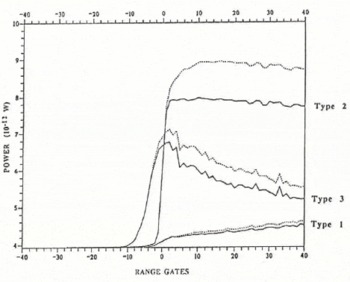
Fig. 8. Examples of modeled echoes with the surface component only (full line) and the volume component (dashed line). Note that the surface component is set to its minimum value and that the apparent ratio volume/surface is then a maximum. The type 1 echo if an example of an echo from a strong off-nadir pointing angle; type 2 represents a flat trailing-edge echo pattern, and type 3 is a “specular echo” pattern. Values for snow density, grain radius and snow temperature are 0.45 Mg m−3, 1.00 mm, −40° C, respectively. The values of surface parameters are different for each modeled echo. The type 3 modeled echo arrives in advance because these values are very large.
The radius of snow grains can evolve with time, because of compaction and aggregation phenomena, and can reach values larger than usual. Figure 9 shows the behavior of the volume-scattering power according to this parameter. Temperature and density have been fixed to respectively −40° C and 0.45 Mg m−3. It can be seen that, for large values of the grain radius, the curve reaches an asymptote, around −2.5 dB, which can be considered as an upper threshold for the volume component.

Fig. 9. Behavior of the volume back-scatter coefficient as a function of the snow-grain radius, for snow temperature of −40° C and density of 0.45 Mg m−3.
VII. Induced Error from The Volume Component on The Re-Tracking Technique
We have shown that the volume component affects the wave-form shape and more especially its trailing edge. It is therefore a priori expected that a leading-edge re-tracker will be more adequate for estimating the surface height.
We have estimated the influence of the volume echo on the surface-height determination using the three re-tracking methods. Table 1 gives the average effect and its standard deviation for the whole bank of 20 wave forms. It is always lower than half a gate. This effect has to be added to the initial re-tracking error due to the surface echo. As previously seen, the different re-tracking methods always define an elevation lower than the real one (Fig. 5). The volume component also induces an error in the same direction (Table 1). At first sight, the most adequate re-tracking method remains the fitting process developed by Reference Martin, Zwally, Brenner and BindschadlerMartin and others (1983). For the same reason as previously, the dispersion in the OCOG method is close to half a gate.
Table 1. Average influence and its standard deviation of the volume echo on the surface-height retrieval for the three different re-tracking algorithms, fitting process, OCOG and GRGS. These values have been calculated using a bank of 20 simulated wave forms with different values of the parameters (see text). They are expressed in gate numbers and in centimeters

In Figure 10, the volume effect induced by the different methods is plotted against the volume/surface ratio. Contrary to intuition, larger errors are induced by lower ratios. Indeed, as can be seen in Figure 7, for large volume echoes, the leading edge is straighter and closer to the middle of the receiving window. Thus, when volume-scattering is important, the estimation of the middle of the leading edge of the wave form and hence the retrieval of the height are not affected too much. Note also that full wave-form re-tracking techniques, in particular the GRGS algorithm, are less sensitive to this volume/surface ratio, because they take into account the whole signal.

Fig. 10. Volume-induced errors for the three re-tracking algorithms: fitting process, OCOG and GRGS as a function of the volume/surface ratio. Values are given for varying off-pointing angles in degrees. Note that the greatest errors appear for the lower ratios.
On the other hand, the result depends on the off-nadir pointing angle. The greatest errors are induced by the higher off-nadir angles even if the volume/surface ratio is low. As a matter of fact, for large off-nadir pointing angles, the wave-form shape is strongly dependent on the antenna gain. The return is characterized by a long, attenuated leading edge. Although the volume echo is small in this case, its effect on height retrieval is large, because it affects the end of the leading edge, which is already hazy. Note that the pure surface re-tracking error is also greater for type 1 wave forms (see Fig. 6). On the other hand, for low off-nadir pointing angles, the leading edge of the surface component is almost vertical. Then, the width and slope of the leading edge of the surface component is almost vertical. Then, the width and slope of the leading edge practically remain insensitive to the volume effect. In this case, the total error during re-tracking is very low, whatever the re-tracking technique.
VIII. Conclusion
We have analyzed the accuracy of the various techniques of satellite-altimeter echo analysis for determining the elevation of continental ice sheets.
The echo wave forms are mostly affected by surface effects, in particular, the off-nadir pointing angle — or equivalently by the surface slope—and by the surface roughness. The modeled power return due to volume back-scatter by the snow cover does not exceed −2.5 dB for acceptable values of snow grain-size, temperature and density, and affects mostly the trailing edge of the echo wave form. Thus, for all existing algorithms used to estimate the surface height from the echo wave form, the error due to volume back-scatter is lower than 50 cm. However, both surface and volume effects are less significant on the leading edge of the wave form so that algorithms that use a model function to search for the middle of this leading edge are more appropriate to determine the altimetric surface height. In particular, the method proposed by Reference Martin, Zwally, Brenner and BindschadlerMartin and others (1983) presents biases lower than 2 ± 2 cm due to surface effects and of the order of −20 ± 20 cm due to volume effects. We strongly recommend that such a method be applied to the ERS-1 data, as proposed by the group of ice-sheet investigations approved by ESA to receive the altimetric data (personal communication from R. Thomas).
In addition to surface elevation, as well as the back-scatter coefficient (Reference Remy and MinsterRemy and others, 1990), the extraction of other parameters from altimeter-radar wave forms is difficult because of the large number of unknown parameters. Figure 11 shows two wave forms simulated with totally different surface and volume parameters, but which are quite similar whether on their leading or on their trailing edges. The power integrals are also almost equivalent. Estimating geophysical parameters (snow grain-size, surface roughness) from the radar echo are then strongly under-determined. In particular, estimation of the volume component from the wave form would be difficult. The altimetric height error due to this component cannot be derived from the re-tracking method. A height bias of the order of 20 ± 20 cm could always be present due to this effect.

Fig. 11. Two similar radar wave forms simulated for very different values of the snow density, grain-size and temperature (values on the upper righthand side) as well as of the surface parameters (pointing angle, r.m.s. of the sastrugi and undulation amplitude; values on the lower righthand side).
One of the altimetric parameters that could have a strong effect on the volume echo is the radar frequency. Figure 12 shows a wave form with constant snow-parameter values, for different radar frequencies. For frequencies higher than 13.5 GHz, the scattering volume is increased by radar-penetration depth decreases. The leading edge of the wave form is therefore narrower and the signal comes mainly from the upper layers. In that case, the accuracy of the surface elevation should probably be better. Conversely, using two-frequency altimeters could help in separating the various effects.

Fig. 12. Volume echoes modeled for different radar frequencies.
Acknowledgements
This work was supported by a CNES Research and Development grant. An original version of the software has been provided by E. Thouvenot from CNES. He is thanked for his help in the commencement of this work. Dr C. Rapley is also thanked for his comments. An extensive review by Dr R. Thomas and an anonymous reviewer have been most helpful.
The accuracy of references in the text and in this list is the responsibility of the authors, to whom queries should be addressed.


