


1. Introduction
Global-climate-model studies have indicated high sensitivity of both ice extent and ice volume to CO2-induced warming, and so hinted at the possibility of early detection of climate change through monitoring of ice-edge position and ice thickness (Reference Parkinson, Weller, Wilson and SeverinParkinson, 1991). Indeed, Reference Gloersen. and Campbell.Gloersen and Campbell (1991) found a small decrease in remotely sensed Arctic ice extent between 1978 and 1987, while Reference Wadhams.Wadhams (1990) showed provocative evidence of a decrease in submarine-measured ice thickness north of Greenland between 1976 and 1987. On the other hand, Reference McLaren, Walsh, Bourke, Weaver. and Wittmann.McLaren and others (1992) compared mean thickness observed at the North Pole in the spring of six years between 1977 and 1990, and found large inter-annual variability with no significant trend. Finally, Reference Chapman, Welch, Bowman., Sacks. and Walsh.Chapman and others (1994) used a version of Reference HiblerHibler’s (1979) “two-level” sea-ice model, forced with observed inter-annually varying forcing from 1960 to 1988, to illustrate the large inter-annual variability inherent in the Arctic ice cover, the persistence of ice-thickness anomalies and the ability of a model to reproduce the apparent decrease in thickness observed by Reference Wadhams.Wadhams (1990) as part of the modelled inter-annual variability. Certainly a more systematic program to measure ice thickness would be valuable to establish ice thickness climatologies and variability against which to gauge future changes and to validate and improve sea-ice models.
In the present work we investigate sea-ice variability using a model which simulates the evolution of the entire thickness-distribution function, and forcing data which cover the period 1951–90. To the extent that the model is capable of reproducing the evolution of the real ice cover, this 39 year time series of ice thickness fields allows us to illustrate certain aspects of spatial and temporal variability relevant to monitoring Arctic ice thickness and ice volume.
2. Model Description and Forcing Data
The model used here is the same as that described by Reference Flato and HiblerFlato and Hibler (in press), based on an earlier model of Reference HiblerHibler (1980), so it will be described only briefly. The ice thickness distribution, g(h), is defined as (Reference Thorndike, Rothrock, Maykut. and ColonyThorndike and others, 1975)

where h is ice thickness, R is the total area of some fixed region, R, about the point of interest, and r(h 1, h 2) is the area in R covered by ice whose thickness is between h 1 and h 2. That is, g(h) can be thought of as the normalized probability density function of ice thickness. This thickness-distribution function evolves according to (Reference Thorndike, Rothrock, Maykut. and ColonyThorndike and others, 1975)

where u is the ice velocity, f is the thermodynamic growth rate, ψ is the so-called redistribution function, and F L is a source term (added by Reference HiblerHibler 1980) which describes the change in thickness distribution due to lateral melting. The redistribution term, ψ a functional of h and g(h), determines the changes in g(h) during a deformation event, essentially “redistributing” ice between thickness categories. The velocity field is obtained by solving the sea-ice momentum equation with the viscous-plastic, elliptical yield-curve theology of Hibler (1979) and the strength parameterized in terms of mechanical energy losses during ridging (Reference RothrockRothrock, 1975). The total mechanical energy dissipation rate is taken to be 17 times the potential energy change as determined by Reference Flato and HiblerFlato and Hibler (in press) from buoy-drift comparisons (this value is similar to that determined by Hopkins (1994) from simulations of individual ridging events). The thickness distribution is represented by 28 fixed thickness categories, closely spaced near the thin end of the distribution and progressively coarser for thicker ice with separate distributions for ridged and level ice (Reference Flato and HiblerFlato and Hibler, in press). The model includes snow accumulation on the ice, with average monthly snowfall rates obtained from the Russian ice-station data from 1957–61 reported in Reference Vowinckel., Orvig. and Orvig.Vowinckel and Orvig (1970). The thermodynamic growth rate is obtained from a surface energy-budget calculation essentially the same as that of Reference Parkinson and Washington.Parkinson and Washington (1979), as described in Reference HiblerHibler (1980), and the Reference SemtnerSemtner (1976) “Zero-layer” heat-conduction formulation. Further details can be found in Reference Flato and HiblerFlato and Hibler (in press).
The model uses a 160 km rectangular grid, shown in Figure 1, and is forced with daily geostrophic winds constructed from surface pressure analyses archived at the U.S. National Center for Atmospheric Research, and augmented by Arctic Buoy Program pressure fields north of 70°N after 1979 (Reference Chapman, Welch, Bowman., Sacks. and Walsh.Chapman and others, 1994). Monthly surface air temperatures are from the University of East Anglia, U.K. (Reference Jones, Raper, Bradley, Diaz, Kelly. and Wigley.Jones and others, 1986), and consist of monthly temperature anomalies, where available, super-imposed upon monthly climatology. Because the anomalies are derived from weather-station records, there are generally none available over the central Arctic and so the modelled ice cover experiences inter-annually varying air temperatures only near the coast. Furthermore, the binning procedure used to construct the anomaly data produces spurious warm temperatures over sea ice in the summer, causing unrealistic melt. Observations from Russian ice camps (e.g. Vowinckel and Orvig, 1970) show that air temperatures over sea ice rarely exceed the freezing point in summer (the maximum ice-surface temperature). Therefore the air temperatures are modified by not allowing temperatures greater than 0.5°C in grid cells where the ice concentration is greater than 15%. Down-welling long-wave radiation is calculated from air temperature and cloud amount using the parameterization of Reference Maykut and ChurchMaykut and Church (1973); short-wave radiation is obtained from the Reference ZillmanZillman (1972) clear-sky formulation along with the same cloud modification used by Reference Chapman, Welch, Bowman., Sacks. and Walsh.Chapman and others (1994). Monthly climatological cloud amounts are taken from Reference Ebert and Curry.Ebert and Curry (1993). Average monthly ocean-surface currents and heat fluxes are taken from the 40 km resolution coupled ice-ocean simulation of Reference Hibler, Zhang. and PeltierHibler and Zhang (1993).

Fig. 1. Model grid. Each grid square is 160 km on a side. The cross-hatched grid cells indicate outflow boundary points through which ice is free to exit the model domain. The solid black dot indicates the location of the thickness-distribution functions plotted in Figure 2.
3. Results of 39 Year Simulation
Thick, ridged ice evolves very slowly, owing to its long lifetime in the central Arctic, and so the distribution of ridged ice takes 10 years or more to reach equilibrium (Reference Flato and HiblerFlato and Hibler, in press). Therefore, the model was initialized with a thickness-distribution field obtained from a previous simulation of the years 1979–85, then run through the 1951–90 period once and the thickness-distribution field from the end of this run used as an initial condition for the final 1951–90 simulation. The model is effectively in cyclo-stationary equilibrium, and only the results from the final 39 year simulation will be discussed. An example of the thickness distribution at a point in the Beaufort Sea for 30 April 1976 is shown in Figure 2 along with the range in distributions for all Aprils, 1951–90. Also shown for comparison is the thickness distribution observed by U.S.S. Gurnard in the Beaufort Sea during April 1976 (Reference Wadhams. and Horne.Wadhams and Horne, 1980). The general shape of the distribution is reproduced quite well by the model, including the bimodal structure reflecting first-year and multi-year ice. The range in modelled distributions shows that inter-annual variability in the shape of the distribution function is confined to thin ice (less than 3m or so). The shape of the tail of the distribution remains essentially the same, with the mean thickness primarily reflecting the relative amounts of thin, level ice and thick, ridged ice.

Fig. 2. Modelled and observed ice thickness distribution functions at the point indicated in Figure 1. The dashed line is the model result from April 1976; the solid line is an observed thickness distribution from April 1976; and the shaded area indicates the range in modelled thickness distributions for April over the period 1951–90. (a) Linear plot, (b) semi-logarithmic plot.
In order to describe spatial variability, we now focus on the first moment of the thickness distribution, the mean thickness. Decadal averages of winter (January–March) mean thickness fields are shown in Figure 3 and illustrate the substantial changes in thickness buildup pattern that occur, particularly the trend toward thicker ice in the East Siberian Sea. In all decades, the observed zone of thick ice along the Canadian Archipelago and north Greenland coast is reproduced, with the ice generally thicker during the 1980s than during the earlier decades.

Fig. 3. Decadal-average winter (January–Manh) mean ice thickness fields. (a) 1950s, (b) 1960s, (c) 1970s, (d) 1980s. Contour interval is 0.5 m.
One way to monitor Arctic sea-ice volume would be to deploy a network of fixed sensors which measure the ice thickness at their location. The design of such a network would of course aim to measure the maximum signal with the fewest sensors. The placement of measurement sites in such a network depends on the goal of the measurement program. If one was interested in observing inter-annual and short-term variability, the strategy would presumably be to place monitoring sites in regions which exhibit the largest fraction of the overall variability. On the other hand, if one was interested in observing long-term trends in the ice volume, monitoring sites would likely be placed at low-variability sites to reduce the background “noise level” in the observations. To give an idea of where such regions are, Figure 4 shows the variance of February and August ice thicknesses (that is, at each point we compute the variance of the 39 February or August mean thicknesses). The East Siberian Sea again appears as a region of large inter-annual variability. Indeed when one considers the dominant circulation pattern, an anticyclonic gyre in the western Arctic, it appears that high-variability ice is advected off the Siberian Shelf while low-variability ice from the central Arctic is advected into this region.

Fig. 4. Variance of February and August mean ice thickness over the period 1951–90. (a) February, (b) August. Contour interval is 0.2 m2.
Optimal spacing of sites within a monitoring network depends on the correlation structure of the thickness field. The correlation is estimated as

where

and

is the mean thickness at point (x,y) averaged over month k counted from January 1951; N
yr = 39 is the number of years; and ⟨⟩kmon
indicates the average of month k
mon over the N
yr period (k
mon = 1 is January, k
mon = 2 is February, etc.). We have implicitly assumed that the correlation is stationary. The model-derived correlation field, ρ(x,y, ![]() , ỹ), is shown in Figure 5 for several points (
, ỹ), is shown in Figure 5 for several points (
![]() , ỹ), where (
, ỹ), where (
![]() , ỹ) are denoted by the heavy black dots in the figure. The area enclosed by the ρ = 0.7 contour (within which a local measurementFootnote
1
explains about 50% of the variance of the surrounding ice) is generally about 4 × 10⁵ km2. As a crude estimate, take this as the area represented by a local measurement; it would therefore take roughly 20 measurement sites to monitor Arctic ice volume. In estimating the total Arctic ice volume, one would not weight all these sites equally; rather, the weights would be assigned based on the variance/covariance structure of the thickness field through some optimization procedure.
, ỹ) are denoted by the heavy black dots in the figure. The area enclosed by the ρ = 0.7 contour (within which a local measurementFootnote
1
explains about 50% of the variance of the surrounding ice) is generally about 4 × 10⁵ km2. As a crude estimate, take this as the area represented by a local measurement; it would therefore take roughly 20 measurement sites to monitor Arctic ice volume. In estimating the total Arctic ice volume, one would not weight all these sites equally; rather, the weights would be assigned based on the variance/covariance structure of the thickness field through some optimization procedure.

Fig. 5. Correlation of mean ice thickness relative to that at the point indicated by a heavy black dot. Contour interval is 0.1.
Given the correlation structure estimated by the model, one could design an optimal measurement network and estimate the measurement error. However, one might also ask about the temporal variability in the ice volume that would be observed by such a network, and so we will examine briefly the ice-volume time series produced by the model. Figure 6 shows the time series of total ice volume and “thin” ice volume (defined as the volume of ice whose thickness is less than 1 m) in the model domain over the 39 year simulation. Also shown is the anomaly time series constructed by subtracting the average annual cycle. Since the model is forced to be in cyclo-stationary equilibrium, there is no overall trend (the volume at the beginning of 1951 is the same as the volume at the end of 1990); however, there is a change in the mid-1970s from “below-average” to “above-average” total ice volume. How much of this is due to the introduction, in 1979, of Arctic buoy data into the surface pressure fields used to force the model is unknown.

Fig. 6. (a) Time series of total ice volume in the model domain (solid line) and volume anomaly (dashed line) computed by subtracting the average annual cycle from the volume time series. (b) Thin-ice ( < 1m) volume and volume-anomaly time series.
The temporal auto-correlation function (ACF) of ice-volume anomaly is shown in Figure 7 for total and thin ice as well as for “medium” thickness ice (defined as thickness of 2–5 m). One can estimate a correlation time-scale by fitting an exponential to the initial decaying part of each ACF (recall that the ACF of a first-order auto-regressive processFootnote 2 is an exponential function; e.g. Jenkins and Watts, 1968). This yields time-scales of approximately 7 years for total ice volume, 20 months for medium-ice volume and 2 months for thin ice volume. The short time-scale associated with thin ice variability reflects the fact that such ice is primarily formed by freezing of open water in newly exposed leads and is subsequently destroyed by ridging; both events coincide with the passage of synoptic systems across the Arctic. Thin ice, however, accounts for only about 5% of the total volume, and so the overall behavior is dominated by thicker ice. Ice thicker than 5m is Formed almost exclusively by ridging, and accounts on average for just under half of the total ice volume. Once formed, such ice can survive the summer melt and remain in the central Arctic for many years before exiting through Fram Strait. Roughly 10–20% of the total Arctic ice volume is transported through Fram Strait each year, implying a renewal time of 5–10 years. A several-year time-scale is also expected from the slow evolution of ridged ice volume noted by Reference Flato and HiblerFlato and Hibler (in press).
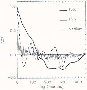
Fig. 7. Auto-correlation functions of total, medium-(2m≤ h ≤5m) and thin-ice (h ≤ 1m) volume-anomaly time series.
4. Discussion and Conclusions
Sea-ice extent and volume represent observable measures of the climatic state in the polar regions. Ice extent has been routinely monitored by satellite imagery for about 20 years; however, ice volume would be a more useful quantity to monitor since it is directly related to heat and fresh-water storage. The technology to observe ice thickness (volume per unit area) using moored upward-looking sonar devices is available and motivates the analysis of modelled ice thickness performed here. Using a fairly comprehensive sea-ice model forced with daily varying winds and monthly mean air temperatures from 1951 to 1990, we computed monthly-average ice thickness fields over the Arctic Ocean and peripheral seas and examined aspects of the spatial and temporal variability.
Regions exhibiting the largest inter-annual variability were the Beaufort Sea and the Siberian Shelf. The Laptev Sea and central Arctic were much less variable. Interestingly, Reference Flato and HiblerFlato and Hibler (in press) found that the Beaufort Sea and Siberian Shelf areas experienced substantially more ridging than the Laptev Sea or central Arctic, and so much of the inter-annual variability may result from differences in wind-driven ridging, firming thick ice which survives several years. The spatial correlation fields showed areas, surrounding a point, of about 4 × 10⁵ km2 in which the correlation coefficient was above 0.7. This sort of information could be used in the design of an ice-thickness monitoring network. Insofar as the modelled ice volume time series are representative of the real Arctic, we would anticipate a temporal correlation time-scale of roughly 7 years for total ice volume, 2 years for the volume of ice between 2 and 5 m thick and 2 months for the volume of ice less than 1 m thick. Particularly for total ice volume, this serial correlation must be taken into account in statistical tests aimed at detecting a trend (see, e.g., Reference Laumann and Gates.Laurmarnn and Gates (1977) for a more complete discussion of the issues involved) and make it unlikely that ice volume will provide an “early” indication of climate change. Detection of trends in ice-covered areas may be more feasible in this regard, since the correlation time-scale of ice-area anomalies is only about 3 months, a time-scale associated with heat storage in the marginal ice-zone mixed layer (Reference Lemke, Trinkl and Hasselmann.Lemke and others, 1980). That is not to say that one should neglect systematic ice thickness monitoring. Indeed, measurement of ice thickness (in fact, the ice thickness distribution function) is vital for the validation of sea-ice models used in global climate simulations, in terms of their ability to reproduce both observed climatological thickness patterns and realistic inter-annual variability.
Acknowledgements
I am grateful to F. Zwiers for many helpful discussions on statistics. I thank W. Chapman for kindly providing the surface-pressure and air-temperature data and B. van Hardenberg for writing programs to interpolate data to the model grid. F. Zwiers, J. Cherniawsky, D. Rothrock and an anonymous reviewer provided valuable comments on the draft manuscript.


