


1. Introduction
Simulations of wall-bounded turbulence at high Reynolds numbers are computationally challenging because they must resolve a vast range of scales. For example, in the near-wall region, the velocity scales with the viscous length scale, which at high Reynolds numbers requires a very fine mesh near the wall. In large-eddy simulations (LES), ‘wall models’ are deployed to model rather than resolve these small near-wall length scales. Wall models for LES have been reviewed in Piomelli & Balaras (Reference Piomelli and Balaras2002), Piomelli (Reference Piomelli2008), Larsson et al. (Reference Larsson, Kawai, Bodart and Bermejo-Moreno2016) and Bose & Park (Reference Bose and Park2018). Here, we concentrate on ‘wall-stress models’ in which the LES domain extends all the way to the wall, where the wall stress is applied as a boundary condition. The simplest and most commonly used wall-stress model is the equilibrium wall model (EQWM), which assumes that the velocity profile follows some known functional form, an equilibrium velocity profile such as the log law (Deardorff Reference Deardorff1970; Schumann Reference Schumann1975; Piomelli et al. Reference Piomelli, Ferziger, Moin and Kim1989). While, strictly, such profiles tend to be valid after long-time averaging under full equilibrium conditions, applications of the EQWM in LES usually assume such profiles to be valid locally and instantaneously. This enables us to use the LES velocity at the wall-model height to determine the local friction velocity and thus the local wall stress. However, the application of a model derived from pure equilibrium assumptions to situations in highly non-equilibrium conditions poses conceptual and practical problems. One difficulty is that it combines both quasi-equilibrium and non-equilibrium effects in a single model formulation, where non-equilibrium effects tend to be clouded by the underlying quasi-equilibrium dynamics. Alternative recent wall models such as the dynamic slip wall models impose a slip velocity boundary condition (Bose & Moin Reference Bose and Moin2014; Bae et al. Reference Bae, Lozano-Durán, Bose and Moin2019). Close connections between slip-velocity and equilibrium wall models have been pointed out in Yang, Bose & Moin (Reference Yang, Bose and Moin2016).
Existing wall models tend to model non-equilibrium and quasi-equilibrium effects in a single formulation. A popular method for incorporating non-equilibrium effects is to solve the full thin boundary layer equations in a near-wall mesh, given the LES velocity (Balaras, Benocci & Piomelli Reference Balaras, Benocci and Piomelli1996). Although this method includes all non-equilibrium terms in the momentum balance, its computational cost can approach that of wall-resolved LES since a refined near-wall mesh is used. Chung & Pullin (Reference Chung and Pullin2009) developed a model based on the wall-normal integrated thin boundary layer equations within the near-wall region and a law of the wall assumption for the velocity profile. Certain non-equilibrium effects can be captured since all terms are included in the momentum balance and because the horizontal Reynolds-stress gradients are evaluated using the subgrid scale (SGS) stresses at the wall-model height. Nevertheless, the model assumes a plug-flow profile for the advection term. In order to account for the velocity profile below the wall-model height, Yang et al. (Reference Yang, Sadique, Mittal and Meneveau2015) developed another wall model (called iWMLES) based on the integrated momentum equations. They assume that the near-wall velocity profile is linear in the viscous sublayer, above which it obeys the log law with an additional linear term to capture non-equilibrium effects. Tests using iWMLES in non-equilibrium flows such as flow over cubed roughness elements (Yang et al. Reference Yang, Sadique, Mittal and Meneveau2015) and the sudden spanwise pressure gradient (SSPG) flow in Lozano-Durán et al. (Reference Lozano-Durán, Giometto, Park and Moin2020) have shown that the model captures properly some non-equilibrium effects. However, iWMLES models non-equilibrium solely through modifying the assumed velocity profile, still assuming that non-equilibrium dynamics can be captured via an only slightly modified equilibrium velocity profile. Thus equilibrium and non-equilibrium effects are mixed together in a single formulation, and it remains unclear how to proceed for more complex flows where the modelling assumption of a near-equilibrium velocity profile is expected to break down.
Recently, a formal approach to separate equilibrium, quasi-equilibrium and highly non-equilibrium conditions for wall modelling was proposed in Fowler, Zaki & Meneveau (Reference Fowler, Zaki and Meneveau2022). The formalism decomposes LES information into contributions from different time scales, and models each component separately. Quasi-equilibrium is assumed to hold for time scales slow enough so that the corresponding velocity profile satisfies the law of the wall. An evolution equation for the friction-velocity vector was derived, which may be described as a ‘Lagrangian relaxation towards equilibrium’, or LaRTE for short. This LaRTE model then captures solely the quasi-equilibrium dynamics, leaving non-equilibrium dynamics to be modelled separately. Consequently, the LaRTE equation was supplemented with a laminar non-equilibrium (lamNEQ) model to capture the wall-stress response to fast changes in the pressure gradient. This combination captures the slow wall-stress behaviour by the LaRTE model, and captures the fast wall-stress behaviour by lamNEQ. The LaRTE+lamNEQ wall model was applied to standard equilibrium channel flow to compare with data and to document the various properties of the approach. Then it was applied to simulate a strongly non-equilibrium flow, the SSPG test case of Lozano-Durán et al. (Reference Lozano-Durán, Giometto, Park and Moin2020), to demonstrate how the model behaves during non-equilibrium conditions.
The Fowler et al. (Reference Fowler, Zaki and Meneveau2022) model, summarized here in § 2, included quasi-equilibrium evolution (slow time scales, of the order of the integral scale turnover time) as well as very fast laminar viscous sublayer dynamics very near the wall. However, the approach did not represent turbulent fluctuations that would arise due to eddies of sizes below the wall-model height, evolving at turbulent time scales represented by the smallest resolved LES motions near the wall. The first objective of the present paper is to introduce a new model turbNEQ for the turbulence portion that was not included before (see § 2.3). The resulting model will thus include three separate parts (LaRTE, lamNEQ and turbNEQ), and be termed the multi-time-scale (MTS) wall model.
While in general non-equilibrium may refer to any flow where the time derivative and/or nonlinear advection terms in the ensemble-averaged momentum balance are non-negligible, in this work we consider only non-stationary flows. Examples considered previously in the direct numerical simulations (DNS), LES and experimental literature include flows with spanwise wall movements in time such as wall oscillations (Jung, Mangiavacchi & Akhavan Reference Jung, Mangiavacchi and Akhavan1992; Quadrio & Ricco Reference Quadrio and Ricco2003; Ricco et al. Reference Ricco, Ottonelli, Hasegawa and Quadrio2012; Yao, Chen & Hussain Reference Yao, Chen and Hussain2019), flows where a spanwise pressure gradient is applied suddenly (Moin et al. Reference Moin, Shih, Driver and Mansour1990; Lozano-Durán et al. Reference Lozano-Durán, Giometto, Park and Moin2020), flows with streamwise acceleration or deceleration (He, Ariyaratne & Vardy Reference He, Ariyaratne and Vardy2008, Reference He, Ariyaratne and Vardy2011; He & Ariyaratne Reference He and Ariyaratne2011; Jung & Chung Reference Jung and Chung2012; He & Seddighi Reference He and Seddighi2013, Reference He and Seddighi2015; Talha & Chung Reference Talha and Chung2015; Jung & Kim Reference Jung and Kim2017; Sundstrom & Cervantes Reference Sundstrom and Cervantes2018c; de Wiart, Larsson & Murman Reference de Wiart, Larsson and Murman2018), and flows with a streamwise oscillating pressure gradient (Tardu, Binder & Blackwelder Reference Tardu, Binder and Blackwelder1994; Scotti & Piomelli Reference Scotti and Piomelli2001; Weng, Boij & Hanifi Reference Weng, Boij and Hanifi2016; Sundstrom & Cervantes Reference Sundstrom and Cervantes2018b; Cheng et al. Reference Cheng, Jelly, Illingworth, Marusic and Ooi2020).
A second objective of this paper is to apply and explore the performance of the MTS wall model for two non-stationary non-equilibrium flows, in which the unsteadiness is applied in the streamwise direction as opposed to the case presented by Fowler et al. (Reference Fowler, Zaki and Meneveau2022), who examined a sudden change in the spanwise pressure gradient. The first application that we consider is pulsating (or oscillating) channel flow (see § 3), where the streamwise pressure gradient forcing oscillates sinusoidally, based on the work of Weng et al. (Reference Weng, Boij and Hanifi2016). The second flow considered in this work is linearly accelerating channel flow (see § 4), where the bulk mean velocity increases linearly during an acceleration period, based on the work of Jung & Kim (Reference Jung and Kim2017). Pulsating and linearly accelerating flows were chosen to apply and explore the new wall model because these flows can cover the vast range of conditions from quasi-equilibrium to highly non-equilibrium flow. For example, for pulsating flow, slow oscillations lead to quasi-equilibrium conditions, whereas fast oscillations lead to non-equilibrium conditions. For linearly accelerating flow, the acceleration rate can be varied to cover different regimes. These flows are interesting application cases because they span various different physical processes, relying on contributions from different parts of the MTS wall model. There is also ample evidence that both of these flows exhibit signs of a laminar Stokes layer during non-equilibrium conditions. For pulsating flow, the periodic wall-stress amplitude and phase follow the Stokes solution (Stokes’ second problem) when the pulsing frequency is very high. For linearly accelerating flow, the deviations of the wall stress and velocity from their initial states follow a laminar solution during the first stage of acceleration if the acceleration is fast enough. Therefore, the lamNEQ model is expected to capture these limiting behaviours. However it is impossible to know a priori how the MTS wall model will perform during conditions in between quasi-equilibrium and laminar non-equilibrium. For these intermediate conditions, the turbulent non-equilibrium model helps to bridge the gap between these two limiting states. Since the wall model used in Fowler et al. (Reference Fowler, Zaki and Meneveau2022) to model rapid spanwise pressure gradient flow did not include the turbulent non-equilibrium (turbNEQ) physics, in Appendix A we briefly revisit that flow as well, showing that predictions using the MTS wall model are comparable to those presented in Fowler et al. (Reference Fowler, Zaki and Meneveau2022) for channel flow subjected to rapid spanwise pressure gradient.
While using the MTS wall model in LES, considerations of model simplicity led us to also explore a simpler option, in which the LaRTE relaxation time scale is set to zero but the model still includes effects from the lamNEQ dynamics. The resulting approach is termed the ‘equilibrium multi-time-scale’ wall model. In § 5, it is shown that it also can provide good predictions of the wall-stress evolution in various applications, but with less complete information about the wall-stress physics. Overall conclusions from this work are discussed in § 6.
2. Multi-time-scale wall model: from full equilibrium to non-equilibrium
We begin with a summary schematic containing all the constitutive parts of the MTS wall model. Figure 1 includes the full spectrum of length and time scales captured in this approach. The wall-modelling region is confined between the wall and the wall-modelling height  $y=\varDelta$, whereas the ‘LES region’ exists above, beyond
  $y=\varDelta$. The total wall stress in the MTS wall model is evaluated as the superposition between the quasi-equilibrium, lamNEQ and turbNEQ components:
 \begin{equation} \boldsymbol{\tau}_w(x,z,t) = \bar{\boldsymbol \tau}_w(x,z,t) + \boldsymbol{\tau}_w''(x,z,t) + \boldsymbol{\tau}_w'(x,z,t).\end{equation}
The quasi-equilibrium component  $\bar {\boldsymbol \tau }_w$ is modelled via the LaRTE wall model first introduced in Fowler et al. (Reference Fowler, Zaki and Meneveau2022) and reviewed in § 2.1. The LaRTE model is named according to its governing equation for the friction-velocity vector
  $\boldsymbol {u}_\tau$, which relaxes to its equilibrium value in a Lagrangian manner at a rate
  $T_s$ called the relaxation time scale. Therefore, the LaRTE model captures the quasi-equilibrium behaviour of the wall stress, which occurs at time scales longer than the relaxation time scale. In figure 1, the LaRTE region is shown in blue, with relaxation represented by the dark blue arrow pointing to the dark grey equilibrium closure region.

Figure 1. Multi-time-scale wall model length and time scales.
The LaRTE model is further supplemented by lamNEQ and turbNEQ models to capture wall-stress dynamics faster than  $T_s$. The lamNEQ component
  $\boldsymbol {\tau }_w''$ covers fast dynamics resulting from the pressure gradient forcing at time scales faster than a viscous time scale,
  $t_\nu \sim \nu /u_\tau ^2$ (where
  $\nu$ is the kinematic fluid viscosity, and
  $u_\tau$ is the friction velocity). This laminar ‘Stokes-like’ behaviour is assumed to be confined to the laminar viscous sublayer. For intermediate time scales, i.e. for time scales between
  $t_\nu$ and
  $T_s$, turbulent eddies that would occur between the wall and
  $y=\varDelta$ but cannot be reproduced by LES must also be modelled. In this paper (§ 2.3), we develop a turbNEQ wall model that completes the spectrum of time scales covered by the MTS wall model.
Generally, the model terms are distinguished by the following notation and colours (abbreviated model name, symbol, colour in parentheses): quasi-equilibrium is marked by overline (LaRTE,  $\bar {\phi }$, blue), laminar non-equilibrium by double prime (lamNEQ,
  $\phi ''$, red), turbulent non-equilibrium by single prime (turbNEQ,
  $\phi '$, green), and full equilibrium by superscript ‘eq’ (
 $\phi ^{eq}$, grey), where
  $\phi$ represents any relevant model variable. Averaging over the homogeneous directions (and ensemble averaging, if applicable) is denoted with angled brackets, with the subscript identifying any additional variables over which averaging is done, i.e.
  $\langle \cdot \rangle$ indicates averaging over
  $x$ and
  $z$, and
  $\langle \cdot \rangle _t$ indicates averaging over
  $x$,
$x$,  $z$ and
  $t$.
$t$.
2.1. Quasi-equilibrium (LaRTE)
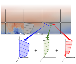
First, we summarize the primary governing equations for the LaRTE portion of the MTS wall model. Derivations and additional details are discussed in Fowler et al. (Reference Fowler, Zaki and Meneveau2022). The goal of the LaRTE portion is to capture quasi-equilibrium dynamics of the wall stress. This is achieved by assuming an equilibrium mean-velocity profile in the near-wall region, whose dimensional parameter (friction velocity) is allowed to evolve slowly in both space and time. Generally, a slow, quasi-equilibrium quantity with LES horizontal resolution is indicated with an overline. For all present applications, we assume that the horizontal quasi-equilibrium velocity  $\bar {\boldsymbol u}_s = \bar {u} \hat {\boldsymbol \imath } + \bar {w} \hat {\boldsymbol k}$ satisfies the law of the wall
 \begin{equation} \bar{\boldsymbol u}_s(x,y,z,t) = {\boldsymbol u}_{\tau}(x,z,t)\,f(y^+),\end{equation}
where  ${\boldsymbol u}_\tau (x,z,t)$ is the friction-velocity vector and is a slowly varying function of the horizontal coordinates
  $(x,z)$ and time
  $t$. A schematic of this velocity profile is shown in figure 2(a). The quasi-equilibrium wall-stress vector can be found from the friction-velocity vector using
 \begin{equation} \bar{\boldsymbol \tau}_w = u_{\tau} {\boldsymbol u}_{\tau}. \end{equation}
Figure 2. A schematic of the velocity profiles for the (a) LaRTE, (b) laminar non-equilibrium, and (c) turbulent non-equilibrium components. Additional visualizations (including an interactive animation) of the various terms comprising the MTS wall model are provided in Appendix A, in figure 27.
LaRTE is based on an evolution equation for the friction-velocity vector  $\boldsymbol {u}_\tau (x,z,t)$, from which the wall stress can then be computed. The evolution of
  $\boldsymbol {u}_\tau (x,z,t)$ is based on an unsteady Reynolds-averaged Navier–Stokes momentum equation for
  $\bar {\boldsymbol u}_s(x,y,z,t)$, the wall-parallel Reynolds averaged velocity as a function of vertical position
  $y$. The momentum balance governing this velocity is
 \begin{align} &\frac{\partial \bar{\boldsymbol u}_s}{\partial t} + \boldsymbol{\nabla}_h \boldsymbol{\cdot} ( \bar{\boldsymbol u}_s \bar{\boldsymbol u}_s ) + \partial_y ( \bar{v} \bar{\boldsymbol u}_s ) ={-} \frac{1}{\rho}\,\boldsymbol{\nabla}_h\bar{p} + \frac{\partial}{\partial y} \left[ (\nu+\nu_T)\, \frac{\partial \bar{\boldsymbol u}_s}{\partial y} \right] \nonumber\\ &\quad + \boldsymbol{\nabla}_h \boldsymbol{\cdot} [(\nu+\nu_T) ( \boldsymbol{\nabla}_h \bar{\boldsymbol u}_s+\boldsymbol{\nabla}_h \bar{\boldsymbol u}_s^{\rm T} )], \end{align}
where  $\boldsymbol {\nabla }_h=\partial _x \hat {\boldsymbol \imath } +\partial _z \hat {\boldsymbol k}$ represents the horizontal gradients on the
  $x$–
$x$– $z$ wall plane, and the total (viscous plus eddy) diffusion cross-terms involving the (small) vertical velocity
  $\bar {v}$ have been neglected. This partial differential equation (PDE) is then integrated vertically from the wall to the wall-model height
  $y=\varDelta$, and the assumed velocity profile (2.2) is substituted to get all terms as a function of
  ${\boldsymbol {u}}_\tau$. After simplifying the PDE, i.e. neglecting horizontal diffusion terms as well as a term representing the horizontal divergence of the friction-velocity direction vector (see Appendix B, which provides an alternative derivation of the LaRTE equation from that presented in Fowler et al. Reference Fowler, Zaki and Meneveau2022), the following evolution equation for the friction-velocity vector is obtained:
 \begin{equation} \frac{\partial {\boldsymbol{u}}_\tau}{\partial t} + {\boldsymbol V}_\tau \boldsymbol{\cdot} \boldsymbol{\nabla}_h {\boldsymbol{u}}_\tau = \frac{1}{T_s} \left[ \frac{1}{u_\tau}\left(-\frac{\varDelta}{\rho}\, \boldsymbol{\nabla}_h \bar{p} + \bar{\boldsymbol{\tau}}_\varDelta \right) - {\boldsymbol u}_\tau\right] + u_\tau\, \frac{\delta^*_\varDelta}{\varDelta}\, \frac{\partial {\boldsymbol s}}{\partial t},\end{equation}
where
 \begin{equation} T_s \equiv f(\varDelta^+)\,\frac{\varDelta }{u_\tau} \end{equation}
appears formally as a relaxation time scale,  $\boldsymbol {s} \equiv \boldsymbol {u}_\tau /u_\tau$ is the unit friction-velocity vector,
 \begin{equation} \bar{\boldsymbol \tau}_\varDelta \equiv \left. (\nu+\nu_T)\,\frac{\partial \bar{\boldsymbol u}_s}{\partial y} \right|_{y=\varDelta}, \end{equation}
is the total shear stress (including viscous and turbulent stresses) at the wall-model height  $y=\varDelta$,
  ${\boldsymbol V}_\tau \equiv (1-{\delta ^*_\varDelta }/{\varDelta } - {\theta _\varDelta }/{\varDelta })\, f(\varDelta ^+)\,{\boldsymbol u}_\tau$ is the advection velocity for the friction-velocity vector, and
 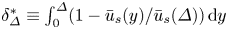 $\delta ^*_\varDelta \equiv \int _0^\varDelta (1-{\bar {u}_s(y)}/{\bar {u}_s(\varDelta )} ) \, {{\rm d} y}$ and
  $\theta _\varDelta \equiv \int _0^\varDelta ({\bar {u}_s(y)}/{\bar {u}_s(\varDelta )}) (1-{\bar {u}_s(y)}/{\bar {u}_s(\varDelta )} ) \, {{\rm d} y}$ are the cell displacement and momentum thicknesses, respectively. In this equation, the friction velocity relaxes in a Lagrangian fashion (with velocity
  ${\boldsymbol V}_\tau$), to its equilibrium value ((2.13), introduced later in this subsection). Hence the model was termed the Lagrangian relaxation towards equilibrium (LaRTE) wall model.
The LaRTE evolution equation is discretized in time using a forward Euler method for explicit evaluation of  $\boldsymbol {u}_\tau$. To evaluate spatial gradients that arise from the advection term in the Lagrangian time derivative, we use a semi-Lagrangian scheme (Staniforth & Côté Reference Staniforth and Côté1991) where the right-hand side of (2.5) is evaluated at the upstream location using bilinear spatial interpolation. The additional numerical diffusion caused by the discretization scheme furthermore reduces the need to evaluate the horizontal diffusion term, thus we opt to neglect it. Specifics for evaluating (2.5) may be found in Fowler et al. (Reference Fowler, Zaki and Meneveau2022).
The term towards which the friction velocity relaxes includes contributions from both the pressure gradient and the total stress at the wall-model height. The LES information (velocity and pressure gradient) contains the full spectrum of time scales resolved by the LES. Therefore, we must remove explicitly the effects of the fast laminar Stokes layer behaviour from the LES inputs, otherwise the friction velocity will relax to an incorrect value. For the quasi-equilibrium pressure gradient, this is done through a one-sided exponential filter that is evaluated as
 \begin{equation} \boldsymbol{\nabla}_h\overline{p}^n = \frac{\delta t^n}{t_\nu}\,\boldsymbol{\nabla}_h p_{LES}^n + \left( 1 - \frac{\delta t^n}{t_\nu}\right) \boldsymbol{\nabla}_h\overline{p}^{n-1},\end{equation}
where  $n$ is the time step index,
  $\delta t$ is the time step size,
  $\boldsymbol {\nabla }_h p_{LES}$ is the LES pressure gradient at the location
  $(x,\varDelta,z)$, and
  $t_\nu$ is a viscous diffusion time scale associated with the laminar Stokes layer. The laminar diffusion time scale
  $t_\nu \sim l^2_s/\nu$ is defined based on the assumption that the laminar Stokes layer is confined to the region from the wall to a height
  $l_s$ in which viscous effects dominate over inertial ones. The thickness of the viscous sublayer is fixed in inner units, therefore we express
  $t_\nu$ in terms of
  $l_s^+= l_s u_\tau /\nu$ according to
 \begin{equation} t_\nu \equiv (l_s^+)^2 \nu/u_\tau^2, \quad {\rm where}\ l_s^+{=} 12. \end{equation}
This viscous time scale represents the time it takes for a Stokes layer to propagate from the wall to the edge of the viscous sublayer. Throughout this paper,  $l_s^+ = 12$ is used. This value marks the intercept between the log law and linear viscous sublayer velocity profiles with the von Kármán constant
  $\kappa =0.4$ and log-law intercept
  $B=5.8$. This value also agrees with the viscous sublayer thickness estimated by Nickels (Reference Nickels2004) (called
  $y_c^+$ in that work).
The total stress at  $y=\varDelta$, i.e.
  $\bar {\boldsymbol \tau }_\varDelta$, is the primary term to be closed in (2.5). The LaRTE wall model uses an equilibrium closure for evaluating the total stress but with a ‘velocity correction’ to the LES velocity that removes the contribution of the laminar Stokes layer to the LES velocity, similar to what was done for the quasi-equilibrium pressure gradient. The total stress closure is based on the full equilibrium momentum balance, where the unsteady and advection terms are set to zero. The smooth-walled, full equilibrium solution is found by solving the ordinary differential equation
 \begin{equation} 0 ={-}\frac{1}{\rho}\,\boldsymbol{\nabla}_h \bar{p} + \frac{{\rm d}}{{\rm d} y}\left( (\nu+\nu_T)\,\frac{{\rm d} \bar{\boldsymbol u}^{eq} }{{\rm d} y}\right),\end{equation}
with boundary conditions
 \begin{equation} \bar{\boldsymbol u}^{eq} (0) = \boldsymbol{0}, \quad \bar{\boldsymbol u}^{eq}(\varDelta) = \bar{\boldsymbol u}_\varDelta, \end{equation}
where  $\varDelta$ is the wall-model height, and
  $\bar {\boldsymbol u}_\varDelta$ is the velocity input to the model. This velocity is related (but not exactly equal) to the LES velocity at
  $y=\varDelta$,
  $\boldsymbol {U}_{LES}$ (as discussed further in this section). The pressure gradient
  $\boldsymbol {\nabla }_h \bar {p}$ is determined from the LES pressure gradient by low-pass filtering it at a viscous time scale, as introduced in (2.8). Finally, the eddy viscosity is assumed to be unaffected by the pressure gradient and is evaluated as
  $\nu _T(y)=[D(y)\,\kappa y]^2\|{\rm d} \bar {\boldsymbol u}^{eq} /{{\rm d} y}\|$, where
  $D(y)$ is the van Driest damping function (van Driest Reference van Driest1956).
Integrating (2.10) between  $y=0$ and
  $y=\varDelta$, one obtains
 \begin{equation} 0 ={-}\frac{\varDelta}{\rho}\,\boldsymbol{\nabla}_h \bar{p} + \bar{\boldsymbol{\tau}}_\varDelta - \bar{\boldsymbol \tau}_w^{eq}, \quad {\rm where} \ \bar{\boldsymbol \tau}_w^{eq} \equiv \left. \nu\,\frac{{\rm d} \bar{\boldsymbol u}^{eq}}{{\rm d} y} \right|_0. \end{equation}
The equilibrium wall stress  $\bar {\boldsymbol \tau }_w^{eq}$ is the viscous stress at the wall involving the solution
  $\bar {\boldsymbol u}^{eq}(y)$ to (2.10). The obtained equilibrium wall stress, appropriately non-dimensionalized, was fitted for general use in Meneveau (Reference Meneveau2020), expressing the result in terms of a wall-model friction factor
  $c_{f}^{wm,eq}(Re_\varDelta,\psi _p)\equiv 2 \bar {\tau }_w^{eq}/\bar {u}_\varDelta ^2$, or equivalently, a wall friction Reynolds number
  $Re_{\tau \varDelta }^{pres}(Re_\varDelta,\psi _p)\equiv \varDelta (\bar {\tau }_w^{eq})^{1/2}/\nu$, where the inputs to the fit are
  $Re_\varDelta \equiv \bar {u}_\varDelta \varDelta /\nu$ and
  $\psi _p \equiv ({1}/{\rho })(\boldsymbol {\nabla }_h \bar {p} \boldsymbol {\cdot } \hat {\boldsymbol e}_u) {\varDelta ^3}/{\nu ^2}$, with
  $\hat {\boldsymbol e}_u \equiv \bar {\boldsymbol u}_\varDelta /\bar {u}_\varDelta$ the velocity input unit vector. Both are related via
  $c_{f}^{wm,eq}=2 [ Re_{\tau \varDelta }^{pres} / Re_{\varDelta } ]^2$ (see Meneveau (Reference Meneveau2020) and Fowler et al. (Reference Fowler, Zaki and Meneveau2022) for more details). Full equilibrium implies that we may use the equilibrium wall model of
  $\bar {\boldsymbol \tau }_w^{eq}$ as a model for the total forcing at
  $y=\varDelta$, namely we replace
 \begin{equation} -\frac{\varDelta}{\rho}\,\boldsymbol{\nabla}_h \bar{p} + \bar{\boldsymbol{\tau}}_\varDelta = \bar{\boldsymbol \tau}_w^{eq} = \frac{1}{2}\, c_{f}^{wm,eq}(Re_\varDelta,\psi_p)\, \bar{u}_\varDelta^2 \hat{\boldsymbol e}_u\end{equation}
in (2.5).
During LES of flows under strong non-equilibrium conditions, we have found that simply using the LES velocity  $\boldsymbol {U}_{LES}$ as the input to the stress closure for
  $\bar {\boldsymbol \tau }_w^{eq}$ (i.e. using
  $Re_\varDelta = U_{LES} \varDelta /\nu$) yields incorrect results during periods of high non-equilibrium forcing. For example, if the flow is accelerated in the streamwise direction by a sudden increase in the pressure gradient, then a shear layer grows near the wall and the velocity outside the shear layer increases. If we were to use the LES velocity as the input, then (2.13) incorrectly attributes the increase in velocity to an increase in the turbulence and the wall stress. Ample evidence from the literature (He & Jackson Reference He and Jackson2000; Greenblatt & Moss Reference Greenblatt and Moss2004; He et al. Reference He, Ariyaratne and Vardy2008; He & Seddighi Reference He and Seddighi2013; Vardy et al. Reference Vardy, Brown, He, Ariyaratne and Gorji2015; Sundstrom & Cervantes Reference Sundstrom and Cervantes2018a) shows that the stress outside of this shear layer remains unchanged for some time after application of the sudden change in the pressure gradient, consistent with the concept of ‘frozen turbulence’. To mimic this effect while also keeping the simplicity of the equilibrium wall model, we correct the LES velocity by subtracting from it the anticipated increase in velocity due to rapid changes in pressure gradient. This velocity correction is denoted as
  $\boldsymbol {u}_\varDelta ''$ and is modelled as the solution to the model equation
 \begin{equation} \frac{\partial \boldsymbol{u}_{\varDelta}''}{\partial t} ={-}\frac{1}{\rho}\,\boldsymbol{\nabla}_h p'' -\frac{\boldsymbol{u}_{\varDelta}''}{T_\varDelta},\end{equation}
where  $T_\varDelta = t_\nu + \varDelta /\kappa u_\tau$ represents the time scale associated with the destruction of the laminar Stokes layer as it diffuses away from the wall. In the absence of mean shear, the fluid acceleration is equal to the pressure gradient. However, because the underlying flow has shear, the laminar Stokes layer above
  $l_s$ weakens and becomes turbulent as it diffuses away from the wall. The characteristic time for this diffusive process to take place,
  $T_\varDelta$, is modelled as the time it takes for the laminar Stokes layer to diffuse to the edge of the viscous sublayer,
  $t_\nu$, plus the eddy turnover time at the wall-model height,
  $\varDelta ^2/\nu _T(\varDelta ) = \varDelta /\kappa u_\tau$. In figures 1 and 2, the dark red region corresponds to the laminar Stokes layer near the wall, which diffuses to the edge of the viscous sublayer,
  $l_s$, by time
  $t_\nu$. The Stokes layer's growth is then interrupted by the turbulent flow, which further diffuses it over an eddy turnover time. This is represented by the light red region in figures 1 and 2. Here,
  $\boldsymbol {\nabla }_h p'' \equiv \boldsymbol {\nabla }_h p_{LES} - \boldsymbol {\nabla }_h \bar {p}$ is the high-pass filtered non-equilibrium pressure gradient containing the high-frequency content of the LES pressure gradient affecting mostly the laminar sublayer dynamics. Equation (2.14) effectively models the changes in the LES velocity due to fast changes in the pressure gradient. Note the similarities between (2.14) and (2.16), soon to be introduced. Equation (2.14) is essentially a model for (2.16) evaluated at the wall-model height
  $\varDelta$ where the viscous term is replaced by a modelled destruction term.
The velocity input used in (2.13) is then given by
 \begin{equation} \bar{\boldsymbol u}_\varDelta = \boldsymbol{U}_{LES} - \boldsymbol{u}_\varDelta''.\end{equation}
The velocity correction  $\boldsymbol {u}_\varDelta ''$ is shown schematically with the thick red vector in figure 2, and the resulting corrected velocity input
  $\bar {\boldsymbol u}_\varDelta$ is shown by the light grey vector. During non-equilibrium events,
  $\boldsymbol {u}_\varDelta ''$ cancels the changes in the LES velocity, which ultimately leads to a delayed response by
  $\bar {\boldsymbol \tau }_\varDelta$. In previous applications of the LaRTE wall model (Fowler et al. Reference Fowler, Zaki and Meneveau2022),
  $\boldsymbol {U}_{LES}$ was filtered using a
  $2\varDelta$ spatial filter to remove LES velocity fluctuations that ultimately lead to an overpredicted wall stress (Bou-Zeid, Meneveau & Parlange Reference Bou-Zeid, Meneveau and Parlange2005). However, we have found that the velocity correction eliminates the need to filter the LES velocity since it inherently removes the high-frequency content in
  $\boldsymbol {U}_{LES}$. Therefore, in the present test cases using the LaRTE wall model, the LES velocity remains spatially unfiltered.
2.2. Laminar non-equilibrium
The lamNEQ wall model developed in Fowler et al. (Reference Fowler, Zaki and Meneveau2022) is based on the concept of frozen turbulence where the Reynolds stresses remain unaffected during a short period after a fast change in the pressure gradient forcing. Since the Reynolds stresses may be neglected, the resulting governing equation for this process is laminar. The lamNEQ velocity  $\boldsymbol {u}''$ is then modelled by solving
 \begin{equation} \frac{\partial \boldsymbol{u}''}{\partial t} ={-} \frac{1}{\rho}\,\boldsymbol{\nabla}_h p'' + \nu\, \frac{\partial^2 \boldsymbol{u}''}{\partial y^2},\end{equation}
where
 \begin{equation} \boldsymbol{\nabla}_h p'' = \boldsymbol{\nabla}_h p_{LES} - \boldsymbol{\nabla}_h \bar{p}\end{equation}
may be interpreted as the high-frequency pressure gradient fluctuations around the LaRTE quasi-equilibrium pressure gradient (see (2.8) for the evaluation of  $\boldsymbol {\nabla }_h \bar {p}$). The resulting flow is confined to a thin region near the wall where the flow is quasi-parallel and advection terms may be neglected, therefore
  ${\boldsymbol \nabla }_h p''$ is the sole driving force for accelerating the flow. The solution to (2.16) is represented in figure 2 by the dark red Stokes layer profile near the wall.
Analytical solutions to (2.16) can be obtained, from which we find the lamNEQ wall stress to be
 \begin{equation} \boldsymbol{\tau}_w''(t) = \sqrt{\nu/{\rm \pi}} \int_{t_0}^t - \frac{1}{\rho}\,\boldsymbol{\nabla}_h p''(t')\, (t - t')^{{-}1/2} \, {\rm d} t'. \end{equation}
Efficient evaluation of (2.18) is challenging due to the non-local nature of the convolution integral. For practical implementation, we use the ‘sum-of-exponentials’ method developed by Jiang et al. (Reference Jiang, Zhang, Zhang and Zhang2017). In this method, the kernel is approximated as a sum of exponential terms
 \begin{equation} (t_n - t')^{{-}1/2} \approx \sum_{m=1}^{N_{exp}} \omega_m \, {\rm e}^{{-}s_m (t_n - t')}, \end{equation}
where the constants  $\omega _m$ and
  $s_m$ are determined a priori. The number of exponential terms,
  $N_{exp}$, is fixed in time, therefore leading to reduced storage and computation requirements. Upon substituting (2.19) into (2.18), one can show that the integral can be evaluated recursively. Exponential time filtering is known to be advantageous because the recursive structure does not require storing the entire time evolution, and the current time-filtered variable depends only on the filtered value at the last time step and the current increment (Meneveau, Lund & Cabot Reference Meneveau, Lund and Cabot1996). The advantage of this method is that it requires
  $O(N_{exp})$ storage and
  $O(N_T N_{exp})$ computational work, whereas a direct method requires storing the entire time evolution, i.e.
  $O(N_T)$ storage and
  $O(N_T^2)$ work, which becomes unwieldy for long simulations. The accuracy of this algorithm was tested and verified in Fowler et al. (Reference Fowler, Zaki and Meneveau2022).
2.3. Turbulent non-equilibrium
The wall-model physics described so far captures the slow, quasi-equilibrium behaviour and the fast, lamNEQ behaviour caused by fast changes in the pressure gradient. The velocities associated with each of these models are governed by (2.2) and (2.14) for the LaRTE and lamNEQ models, respectively. We now introduce a simple model that accounts for the velocity difference between the LES velocity and the LaRTE and lamNEQ models. This velocity deficit is expressed as
 \begin{equation} \boldsymbol{u}_\varDelta' = \bar{\boldsymbol u}_\varDelta - \boldsymbol{u}_\tau\,f(\varDelta^+) = \boldsymbol{U}_{LES} - \boldsymbol{u}_{\varDelta}'' - \boldsymbol{u}_\tau\,f(\varDelta^+),\end{equation}
and is represented in figure 2 by a thick green vector. Turbulent non-equilibrium is assumed to occur when turbulence affects the velocity profile at a rate faster than the relaxation time scale, thus the LaRTE model is unable to account for this effect.
Since  $\boldsymbol {U}_{LES}$ is known from the simulation, and the laminar velocity
  $\boldsymbol {u}_\varDelta ''$ and LaRTE velocity contribution are known from their respective models, during LES, the remainder represents the turbulence that is left out and not yet included in the wall model. While this velocity can be computed during LES based on (2.20), what remains is to determine the contribution to the wall stress from turbulent flow structures that are associated with the velocity fluctuation
  $\boldsymbol {u}_\varDelta '$. For this purpose, we invoke the attached eddy hypothesis of Townsend (Reference Townsend1976), which has been refined further in various more recent works (Mathis, Hutchins & Marusic Reference Mathis, Hutchins and Marusic2009; Smits, McKeon & Marusic Reference Smits, McKeon and Marusic2011; Marusic & Monty Reference Marusic and Monty2019). Based on the attached eddy hypothesis,
  $\boldsymbol {u}_{\varDelta }'$ may be viewed as a turbulent velocity fluctuation caused by the large, wall-attached eddies with height of the order of
  $\varDelta$, as portrayed in figure 3. We are interested only in the wall stress filtered to the LES resolution, i.e. the local average of effects of eddies over the LES resolution. It is this local average that is associated with the velocity fluctuation
  $\boldsymbol {u}_\varDelta '$. The contribution of eddies smaller than
  $\varDelta x \times \varDelta \times \varDelta z$ is neglected. In the absence of additional information or any further assumptions, we model the resulting flow structures as consisting of streamwise elongated high- and low-speed regions in which the velocity profile is approximated as mostly plug flow. When approaching the wall, one assumes that there is a linear shear layer connecting the profile to the no-slip boundary condition on the smooth wall. We assume that this layer has the thickness of the viscous sublayer (the same as that assumed for the Stokes layer,
  $l_s$). The turbNEQ velocity is then
 \begin{equation} \left.
\begin{array}{ll@{}} \boldsymbol{u}' =
\boldsymbol{u}_\varDelta'\, \dfrac{y}{l_s} & \textrm{for} \
0 \leq y \leq l_s, \\ \boldsymbol{u}' =
\boldsymbol{u}_\varDelta' & \textrm{for} \ y \geq
l_s, \end{array}\right\} \end{equation}
\begin{equation} \left.
\begin{array}{ll@{}} \boldsymbol{u}' =
\boldsymbol{u}_\varDelta'\, \dfrac{y}{l_s} & \textrm{for} \
0 \leq y \leq l_s, \\ \boldsymbol{u}' =
\boldsymbol{u}_\varDelta' & \textrm{for} \ y \geq
l_s, \end{array}\right\} \end{equation}
where  $l_s = l_s^+ \nu /u_\tau$ with
  $l_s^+=12$, and the friction velocity
  $u_\tau$ comes from the LaRTE model. The wall stress is then computed as
 \begin{equation} \boldsymbol{\tau}_w' \equiv \left. \nu\, \frac{\partial \boldsymbol{u}'}{\partial y} \right|_0 = \frac{u_\tau \boldsymbol{u}_\varDelta'}{l_s^+}.\end{equation}
Very recently, Hansen et al. (Reference Hansen, Whitmore, Abkart and Yang2022) have shown that very similar vertical profiles can be obtained from proper orthogonal decomposition analysis, showing that the most important (energetic) modes of the unresolved turbulence can be described by plug flow with a viscous layer towards the wall starting at  $y^+ \sim 12$, consistent with our simple model.

Figure 3. A schematic of the turbNEQ velocity profiles resulting from two counter-rotating wall-attached eddies. Circles indicate the LES grid points, and the blue surface indicates a possible region of negative velocity fluctuation (green arrows) induced between wall-attached eddies (yellow) that can be only partially resolved on the LES resolution.
2.4. Summary of the MTS wall model
The total wall stress for the MTS wall model is evaluated as the superposition of the three components according to (2.1), where  $\bar {\boldsymbol \tau }_w = u_\tau \boldsymbol {u}_\tau$ is the quasi-equilibrium/LaRTE wall stress governed by (2.5),
  $\boldsymbol {\tau }_w''$ is the lamNEQ wall stress governed by (2.18), and
  $\boldsymbol {\tau }_w'$ is the turbNEQ wall stress governed by (2.22). The LaRTE model has two inputs, the quasi-equilibrium pressure gradient
  ${\boldsymbol \nabla }_h\bar {p}$, and the quasi-equilibrium velocity
  $\bar {\boldsymbol u}_\varDelta$, needed for the equilibrium stress closure that is evaluated as a wall-model friction factor according to (2.13). Dynamics occurring faster than a viscous time scale
  $t_\nu$ (see (2.9)) is assumed to contribute to a laminar Stokes layer that is confined to the laminar viscous sublayer near the wall. The laminar viscous sublayer thickness is fixed in inner units (we use
  $l_s^+ = 12$ throughout the paper). Dynamics occurring faster than
  $t_\nu$ must be removed from the inputs to the equilibrium stress closure, otherwise the predicted stress will be incorrect. For the quasi-equilibrium pressure gradient, this is done by filtering explicitly the LES pressure gradient according to (2.8). For the quasi-equilibrium velocity, the LES velocity
  $U_{LES}$ must be corrected by subtracting from it the estimated change in velocity due to fast laminar Stokes layer dynamics. The velocity correction is modelled according to (2.14), which is then subtracted from the LES velocity to get the velocity input according to (2.15).
The lamNEQ model captures wall-stress dynamics responding to fast changes in the LES pressure gradient ( ${\boldsymbol \nabla }_h p''$ defined in (2.17)). The resulting governing equation for the lamNEQ wall stress requires evaluating a non-local convolution integral. Efficient evaluation is achieved through the use of a sum-of-exponentials approximation to the kernel, (2.19), where
  $N_{exp}$ terms must be stored per horizontal grid point. This leads to a noticeable but relatively small increase in the computational cost, as discussed at the end of § 5. However, the key point is that the storage requirement remains fixed in time while still accurately capturing wall-stress dynamics operating in this laminar Stokes layer regime, as discussed in the subsequent results sections.
The turbNEQ model captures wall-stress dynamics responding to LES velocity fluctuations not accounted for by the LaRTE and lamNEQ models. This turbNEQ velocity fluctuation ( $\boldsymbol {u}_\varDelta '$ defined according to (2.20)) is predicted to occur in response to wall-attached eddies with sizes similar to the LES grid resolution. To connect the wall-stress response to this velocity fluctuation, we must model the corresponding velocity profile. The velocity profile is modelled as mostly plug flow with a linear shear layer near the wall, with the thickness being the same thickness as the viscous sublayer,
  $l_s$. The turbNEQ wall stress may then be computed according to (2.22).
3. Wall-modelled LES for pulsating channel flow
Large-eddy simulations of pulsating channel flow, with an oscillating streamwise pressure gradient forcing, were conducted with the MTS wall model and with the classical EQWM. These results are compared with the DNS of Weng et al. (Reference Weng, Boij and Hanifi2016) upon which the simulation set-up is largely based. As in Weng et al. (Reference Weng, Boij and Hanifi2016), we adopt a triple decomposition where any variable,  $F(\boldsymbol {x},t)$, may be written as
 \begin{equation} F(\boldsymbol{x},t) = \langle F \rangle_t(y) + \tilde{F}(y,t) + F'(\boldsymbol{x},t), \end{equation}
where  $\langle F \rangle _t$ is the steady, time and horizontally averaged field,
  $\tilde {F}$ is the periodic component caused by the oscillatory pressure gradient, and
  $F'$ corresponds to turbulent fluctuations. Note that the turbulent fluctuations are the only cause for variability in the
  $x$ and
  $z$ directions for channel flow. Also note that a single prime in this section is not to be confused with a turbNEQ quantity unless specified otherwise. The time and horizontally averaged component is computed as
 \begin{equation} \langle F \rangle_t(y) = \frac{1}{(t_{N_t}-t_0) L_z L_x} \int_{t_0}^{t_{N_t}} \int_{0}^{L_z} \int_{0}^{L_x} F(\boldsymbol{x},t) \, \mathrm{d}\kern0.7pt x \, \mathrm{d} z \, \mathrm{d} t, \end{equation}
where  $t_0$ and
  $t_{N_t}$ are the initial and final times, respectively, over which time averaging is done. The periodic component is found by subtracting the time-averaged flow field from the phase average:
 \begin{equation} \tilde{F} (y,t) \equiv \frac{1}{N_p L_x L_z} \sum_{n=1}^{N_p} \int_0^{L_z} \int_0^{L_x} F ( \boldsymbol{x}, t + (n-1) T_f ) \, {\rm d}\kern0.7pt x \, {\rm d}z - \langle F \rangle_t(y), \end{equation}
where  $T_f$ is the pressure gradient forcing period, and
  $N_p$ is the total number of periods over which phase averaging is done.
Simulations are performed using LESGO (an open-source, mixed pseudo-spectral and finite difference code available on github, LESGO 2021) with a steady friction Reynolds number  $\langle Re_\tau \rangle _t = u_{\tau p} h/\nu = 350$, where
  $h$ is the channel half-height, and
  $u_{\tau p} \equiv \sqrt {-h\rho ^{-1}(\partial _x \langle p \rangle _t)}$ is the friction velocity based on the steady pressure gradient. The Lagrangian scale-dependent dynamic subgrid stress model (Bou-Zeid et al. Reference Bou-Zeid, Meneveau and Parlange2005) is used in the bulk of the flow. The domain size, number of grid points and grid size are
  $(L_x, L_y, L_z)/h = (8{\rm \pi},2,3{\rm \pi} )$,
  $(N_x, N_y, N_z) = (128,30,48)$ and
  $(\varDelta _x, \varDelta _y, \varDelta _z)/h = (0.196,0.067,0.196)$, respectively. The third grid point is used for the wall-model height (i.e.
  $\varDelta = 5\varDelta _y/2$) because for low-Reynolds-number simulations, the first grid point falls beneath the log layer where the SGS model lacks accuracy. This underperformance causes an incorrect velocity to be fed into the wall model, which in turn produces an incorrect wall stress. Choosing a point further away allows a more accurately computed velocity to be fed into the wall model. It is also in agreement with the recommendations made by Larsson et al. (Reference Larsson, Kawai, Bodart and Bermejo-Moreno2016). Time advancement is done using an Adams–Bashforth method with a varying time step size to achieve a constant Courant–Friedrichs–Lewy (CFL) value 0.05. On average, this gives a time step size
  $\delta t \approx 4.2\times 10^{-4} h/u_{\tau p}$, which is two orders smaller than the fastest forcing time scale. This assures that all dynamics are well resolved temporally.
Sinusoidal flow variation is caused by the time-periodic streamwise pressure gradient forcing
 \begin{equation} \frac{\partial \langle p \rangle}{\partial x} = \frac{\partial \langle p \rangle_t}{\partial x}\,[ 1 + \beta \cos ( \omega_f t ) ], \end{equation}
where  $\partial \langle p \rangle _t/\partial x$ is the steady pressure gradient forcing, and
  $\omega _f$ and
  $\beta$ are the pressure gradient forcing frequency and amplitude, respectfully. In our simulations, we use a sine function instead of a cosine function to avoid a discontinuous change in the pressure gradient forcing at
  $t=0$ when the forcing starts; however, we adopt the nomenclature of Weng et al. (Reference Weng, Boij and Hanifi2016) which uses a cosine function. Therefore, all phases reported are consistent with a cosine pressure gradient forcing. A wide range of forcing frequencies are tested, which cover the full range of possible flow types. This is summarized in table 1. The forcing frequency determines the extent to which the Stokes layer penetrates into the flow. Similarly, the Stokes length scale provides an estimate of this penetration depth and is related to the frequency through
  $l_f = \sqrt {2\nu /\omega _f}$ or in inner units
  $l_f^+ = \sqrt {2/\omega _f^+}$, where inner units normalization is done with the friction velocity
  $u_{\tau p}$ and the kinematic viscosity
  $\nu$. If the Stokes layer stays within the viscous sublayer, then it does not interact with the turbulence and the flow remains ‘quasi-laminar’. This is estimated to occur when
  $\omega _f^+>0.04$ or
  $l_f^+<7$ (Weng et al. Reference Weng, Boij and Hanifi2016). Several of the other frequencies tested are in the so-called ‘intermediate frequency range’
  $0.006<\omega _f^+<0.04$, where the wall-stress amplitude is actually less than the amplitude from the Stokes solution. Finally, a couple of low-frequency cases are tested where the flow is in a quasi-steady state. In other words, the flow has time to adjust to the instantaneous pressure gradient.
Table 1. The forcing frequencies  $\omega _f^+$ and periods and their corresponding Stokes lengths
  $l_f$ in inner units and outer units, and the flow regime classification. For comparison, the relevant wall-modelling time scales are
  $\langle T_s \rangle _t\,u_{\tau p}/h = 2.57$,
  $\langle t_\nu \rangle _t\,u_{\tau p}/h = 0.41$ and
  $\langle T_\varDelta \rangle _t\,u_{\tau p}/h = 0.83$.

Following Weng et al. (Reference Weng, Boij and Hanifi2016), the pressure gradient forcing amplitude is set to give a constant ratio for the periodic centreline velocity amplitude over the mean centreline velocity. This is done by fixing  $a_{cl} \equiv |\tilde {u}_{cl}|/U_{cl} = 0.1$, where
  $U_{cl}$ is the centreline velocity of the laminar flow with the same flow rate as the turbulent mean flow. The relationship between
  $\beta$ and
  $a_{cl}$ can be determined by finding an analytical expression for the periodic centreline velocity
  $\tilde {u}_{cl}$. This is obtained by writing the momentum balance at the centre of the channel and then neglecting the total periodic stress – a valid assumption if the Stokes layer is far from the centre of the channel. The periodic centreline velocity is then found to be
 \begin{equation} \tilde{u}_{cl} = |\tilde{u}_{cl}| \cos (\omega_f t + \phi_{\tilde{u}_{cl}}), \end{equation}
where
 \begin{equation} |\tilde{u}_{cl}| = \frac{\beta u_{\tau p}^2}{\omega_f h}, \quad \phi_{\tilde{u}_{cl}} ={-} {\rm \pi}/2.\end{equation}
Combining the amplitude shown in (3.6a,b) and the definition of  $a_{cl}$,
  $\beta$ can be found using
 \begin{equation} \beta = a_{cl} \omega_f^+\,Re_{cl}, \end{equation}
where  $Re_{cl}\equiv U_{cl}h/\nu \approx 9078$ for
  $Re_\tau = 350$, and
  $a_{cl}$ is set to a constant value
  $0.1$.
For the figures throughout this paper, the line types and colours of the various models/data have the following forms: DNS are shown with dashed black lines; LES with the MTS wall model are shown with solid black lines; and LES with the EQWM are shown with dashed-dot grey lines. For vertical profiles, open circles and plus symbols correspond to the location of LES grid points for LES with the MTS wall model and the EQWM, respectively. Extraneous lines, such as analytical laminar solutions, are shown with thin dotted lines. The different wall-stress components of the MTS wall model are shown with different colours: total wall stress is black, LaRTE wall stress is blue, lamNEQ wall stress is red, and turbNEQ wall stress is green.
Figure 4 shows the periodic centreline velocity for a wide range of pressure gradient forcing frequencies. For the intermediate and high frequencies, the LES are nearly indistinguishable from the DNS, whereas for  $\omega _f^+ = 0.001, 0.003$, there are some discrepancies. These differences may be attributed to the LES overprediction of the mean velocity in the centre of the channel (see figure 5), which becomes important only for low frequencies when the Stokes layer interacts with the turbulence near the centre of the channel. However, for the intermediate and high frequencies, the centreline velocity agrees quite well with (3.5) and (3.6a,b), and the target periodic centreline velocity amplitude (
 $a_{cl}=0.1$) has been met.

Figure 4. The time evolution of the periodic centreline velocity  $\tilde {u}_{cl}$ for several forcing frequencies,
  $\omega _f^+=0.001, 0.003, 0.006, 0.01, 0.02, 0.04$ (plots (a–f), respectively). Line types correspond to LES using the MTS wall model (thick solid black), LES using the EQWM (thick dashed-dot grey), and DNS from Weng et al. (Reference Weng, Boij and Hanifi2016) (thick dashed black). The phase within the cycle is based on the imposed pressure gradient forcing.

Figure 5. The time-averaged mean (a) velocity profiles and (b) Reynolds stresses. Dashed lines correspond to the DNS of Weng et al. (Reference Weng, Boij and Hanifi2016) for  $Re_\tau =350$ with pulsations; circles with solid connecting lines correspond to LES with the MTS wall model; and plus symbols with dashed-dot connecting lines correspond to LES with the EQWM. In (b),
  $\langle u'u' \rangle _t$,
  $\langle v'v' \rangle _t$,
  $\langle w'w' \rangle _t$ and
  $\langle u'v' \rangle _t$ are shown with blue, red, green and black lines, respectively. For the LES, only the high-frequency case (
 $\omega _f^+=0.04$) is shown since the time-averaged velocity and Reynolds stress profiles are independent of the pulsation frequency.
Figure 5 shows the time-averaged mean velocity profiles and Reynolds stresses for the MTS wall model and for the EQWM compared with the DNS of Weng et al. (Reference Weng, Boij and Hanifi2016). The MTS wall model and the EQWM give nearly identical first- and second-order statistics. This indicates that the mean behaviour of the LES is largely unaffected by the wall-model choice. As discussed in Fowler et al. (Reference Fowler, Zaki and Meneveau2022), there is a slight overshoot in the mean velocity profile in the wake region. However, this overshoot is attributed to simulation details other than the wall model, such as subgrid model and numerical effects. Additionally, for these low Reynolds number simulations, the SGS model tends to underpredict the subgrid stress beneath the log layer, thus leading to an overpredicted velocity. This is evident from the first grid point in figure 5. The Reynolds shear stress agrees well with DNS, as expected from momentum conservation, and the streamwise normal stress is also well predicted (except for the near-wall peak that is unresolved in LES). The spanwise and wall-normal diagonal Reynolds stress profiles are overpredicted by the LES, but in equal measure by all the wall models, pointing to remaining limitations of the SGS closure and not the wall models.
The governing equation for the periodic component of the streamwise velocity is found by subtracting the time-averaged streamwise momentum equation from the phase-averaged streamwise momentum equation:
 \begin{equation} \frac{\partial \tilde{u}}{\partial t} ={-}\frac{1}{\rho}\,\frac{\partial \tilde{p}}{\partial x} + \nu\,\frac{\partial^2 \tilde{u}}{\partial y^2} - \frac{\partial \widetilde{u'v'}}{\partial y}.\end{equation}
Laminar analytical solutions to (3.8) can be found by setting the Reynolds stress term to zero and using  $\partial _x \tilde {p} = \beta (\partial _x \langle p \rangle _t) \cos (\omega _f t)$. The frequencies considered in table 1 are high enough such that the Stokes solution is similar to the laminar channel flow solution since
  $l_f \ll h$, as shown in table 1. Therefore we will simply use the Stokes solution as the ‘laminar channel flow solution’, which is
 \begin{equation} \tilde{u}/U_{cl} = a_{cl} [ \sin(\omega_f t) - {\rm e}^{{-}y/l_f}\sin(\omega_f t - y/l_f) ]. \end{equation}
Figure 6 shows the amplitude and phase of the periodic velocity for the six lowest forcing frequencies. The Stokes solution curve is also shown for reference. In the plots, it is clear that for the lowest frequency, the DNS and LES deviate from the Stokes solution significantly, thus a quasi-laminar state is not achieved. However, for the highest frequency shown, the DNS and LES follow the Stokes solution very closely, thus indicating that the flow is in a quasi-laminar state. Generally, the LES agree closely with the DNS. The MTS wall model and EQWM produce similar results, with the greatest discrepancies between the two occurring in the first few grid points away from the wall. These grid points are more sensitive to the wall model since they are affected more directly by the wall stress.

Figure 6. (a) Amplitude and (b) phase lead of the periodic velocity for six forcing frequencies,  $\omega _f^+ = 0.001, 0.003, 0.006, 0.01, 0.02, 0.04$. The DNS of Weng et al. (Reference Weng, Boij and Hanifi2016), the LES with the MTS wall model, the LES with the EQWM, and the Stokes solution are shown with dashed black lines, open circles connected with solid black lines, grey plus symbols connected with grey dashed-dot lines, and dotted black lines, respectively. Animations of the periodic velocity can be accessed at https://www.cambridge.org/S0022112023005852/JFM-Notebooks/files/Figure-6/u_animation.html, and the corresponding source code can be found at https://www.cambridge.org/S0022112023005852/JFM-Notebooks/files/Figure-6/pulse_velocity_profiles.ipynb. Note that the animations of the DNS velocity profiles are computed from the provided amplitudes and phases.
Figures 7–10 show how the periodic wall stress changes with frequency, where figures 7 and 8 show the periodic wall-stress time signals, and figures 9 and 10 show the periodic wall-stress amplitude and phase as functions of frequency. Figure 7 compares LES with the MTS wall model (solid black lines) against the DNS of Weng et al. (Reference Weng, Boij and Hanifi2016) (dashed black lines), and the LES with the EQWM (dashed-dot grey lines). The figure shows that the MTS wall model and EQWM perform similarly well for low frequencies, but as the frequency is increased, the EQWM degrades in performance, whereas the MTS wall model follows the trends of the DNS quite well. This is expected since the EQWM is based on equilibrium assumptions and therefore cannot capture properly the non-equilibrium dynamics of the high-frequency test cases. Figure 8 shows the different wall-stress contributions in the MTS wall model for the low, intermediate and high frequencies. This figure demonstrates why the MTS wall model can capture the trends of the DNS, and highlights the usefulness of such an approach. For the low, intermediate and high frequencies, the dominant contributors to the periodic wall stress are the quasi-equilibrium (LaRTE), turbNEQ and lamNEQ components, respectively. This is consistent with the length and time scale schematic in figure 1, where each component of the MTS wall model targets dynamics within a range of time scales. Using table 1, we see that the flow dynamics relative to the relaxation time scale (the frequencies in figure 8) are of the orders (a)  $T_f/T_s \gg 1$, (b)
  $T_f/T_s \sim 1$ and (c)
  $T_f/T_s < 1$, which again is consistent with the model picture in figure 1. Note that in this flow, the scale separation between the laminar viscous time scale
  $t_\nu$ and the relaxation time scale
  $T_s$ is not very large (from the caption in table 1, we see that
  $\langle t_\nu \rangle _t/\langle T_s \rangle _t=0.16$). This is a direct result of the low Reynolds number of the flow considered. As seen from the expression
  $t_\nu /T_s = (l_s^+)^2/f(\varDelta ^+)\, \varDelta ^+$, the numerator is constant while typically, the denominator (and thus the scale ratio) increases with increasing Reynolds number.

Figure 7. Single-period time evolution of the periodic streamwise wall stress  $\tilde {\tau }_{wx}$ for several forcing frequencies,
  $\omega _f^+=0.001, 0.003, 0.006, 0.01, 0.02, 0.04$ (plots (a–f), respectively). Line types correspond to LES using the MTS wall model (thick solid black), LES using the EQWM (thick dashed-dot grey), and DNS from Weng et al. (Reference Weng, Boij and Hanifi2016) (thick dashed black). The phase within the cycle is based on the imposed forcing frequency.

Figure 8. Single-period time evolution of the periodic streamwise wall stress  $\tilde {\tau }_{wx}$ for low, intermediate and high forcing frequencies:
  $\omega _f^+=0.001, 0.006, 0.04$ (plots (a–c), respectively). Line types correspond to LES using the MTS wall model (thick solid black), with LaRTE (thin solid blue), lamNEQ (thin solid red) and turbNEQ (thin solid green) parts, and DNS from Weng et al. (Reference Weng, Boij and Hanifi2016) (thick dashed black). The phase within the cycle is based on the imposed forcing frequency.

Figure 9. (a) The periodic wall-stress amplitude normalized by the Stokes solution amplitude. (b) The periodic wall-stress phase relative to the centreline velocity phase. Asterisks correspond to outside experimental, LES or DNS data from Ronneberger & Ahrens (Reference Ronneberger and Ahrens1977) (experimental), Tardu et al. (Reference Tardu, Binder and Blackwelder1994) (experimental), Scotti & Piomelli (Reference Scotti and Piomelli2001) (LES) and Weng et al. (Reference Weng, Boij and Hanifi2016) (DNS). The DNS data of Weng et al. (Reference Weng, Boij and Hanifi2016) are emphasized with filled circles and connected with thick dashed black lines. LES using the MTS wall model are shown with open circles and connected with thick solid black lines. LES using the EQWM are shown with plus symbols and connected with thick dashed-dot grey lines. The thin dotted horizontal black lines correspond to the Stokes solution.

Figure 10. (a) The periodic wall-stress amplitude normalized by the Stokes solution. (b) The periodic wall-stress phase relative to the centreline velocity phase. Line types correspond to the DNS of Weng et al. (Reference Weng, Boij and Hanifi2016) (filled circles connected with thick dashed black lines) and LES using the MTS wall model (open circles connected with thick solid black lines), with LaRTE (open circles connected with thick solid blue lines), lamNEQ (open circles connected with thick solid red lines), and turbNEQ (open circles connected with thick solid green lines) components. The thin dotted horizontal black lines correspond to the Stokes solution.
Figures 9 and 10 show the periodic wall-stress amplitude and phase. They provide the same information as figures 7 and 8, but in a more succinct manner, allowing trends to become more obvious. In general, as the forcing frequency increases, the wall-stress amplitude (normalized with the Stokes solution amplitude) decreases, and the wall-stress phase (relative to the centreline velocity phase) increases, until they reach their Stokes limit values 1 and 45 degrees, respectively. Figure 9 demonstrates clearly that the EQWM is unable to capture the non-equilibrium effects caused by the high-frequency pressure gradient pulsations. The wall-stress amplitude continues to decrease past its Stokes limit value, while the phase remains relatively constant. The MTS wall model, on the other hand, agrees quite well with DNS trends. It even captures the non-monotonic behaviour in the intermediate frequency range where the periodic wall-stress amplitude falls beneath the Stokes amplitude. The wall model's ability to capture the full spectrum of frequencies, from quasi-equilibrium conditions to Stokes limit conditions, is due to the separate modelling of quasi-equilibrium and non-equilibrium effects. This is observed most clearly in figure 10, where the model's decomposition into quasi-equilibrium, lamNEQ and turbNEQ parts is shown. The periodic wall stress, which is the wall-stress deviation from equilibrium conditions, is captured best by the LaRTE model for low frequencies, the lamNEQ model for high frequencies, and the turbNEQ model for intermediate frequencies (since the LaRTE and lamNEQ models become out of phase with each other). These models effectively turn on or off depending on if the conditions consistent with these models are met. This is an important quality to have to capture both extremes of non-equilibrium.
Figures 11–15 show the periodic Reynolds stresses as functions of height and phase for several forcing frequencies. In order to compare LES with DNS, the SGS stresses are included for the shear stress component, although the SGS contribution is negligible relative to the resolved stresses. Figure 11 shows  $\widetilde {u'v'}$ profiles at different times (where time is indicated by a shift in the vertical direction), whereas figure 12 shows the
  $\widetilde {u'v'}$ amplitude and phase. For succinctness, only the amplitude and phase plots are shown for the normal stresses. Unlike the time-averaged Reynolds stress profiles in figure 5, the periodic Reynolds stresses for the wall-model LES do exhibit a dependency on the wall-model choice. For instance, in figure 12(c), the EQWM agrees well with the DNS, whereas the MTS wall model significantly underpredicts the amplitude. This discrepancy (for this particular frequency) is discussed further in detail below. Overall, the LES with the EQWM appear to agree with the DNS better than the MTS wall model for the
  $\widetilde {u'v'}$ and
  $\widetilde {u'u'}$ components; however, the reverse is true for the
  $\widetilde {v'v'}$ and
  $\widetilde {w'w'}$ components, where the EQWM tends to overpredict the amplitudes. It is interesting to note that the discrepancy between the MTS wall model and the EQWM is greatest for the intermediate frequencies and not for the highest frequency. This might be explained by the fact that for these frequencies, the Stokes length is roughly the same height as the height of the first LES grid point, which is the point that is most sensitive to the wall model.

Figure 11. The time evolution of  $\widetilde {u'v'}$ at different phases of the wave cycle for different forcing frequencies:
  $\omega _f^+ = 0.001, 0.006, 0.01, 0.02, 0.04$. The profiles are
  $T_f/32$ apart, and are offset by
  $1\times 10^{-1}$ units in the vertical direction. Grey lines correspond to the DNS of Weng et al. (Reference Weng, Boij and Hanifi2016). Black lines correspond to LES using the MTS wall model. Animations of the different periodic Reynolds stress components can be viewed by clicking on the links corresponding to the following frequencies:
  $\omega _f^+ = 0.001$, https://www.cambridge.org/S0022112023005852/JFM-Notebooks/files/Figure-11/rs_pul1_animation.html;
  $\omega _f^+ = 0.006$, https://www.cambridge.org/S0022112023005852/JFM-Notebooks/files/Figure-11/rs_pul3_animation.html;
  $\omega _f^+ = 0.01$, https://www.cambridge.org/S0022112023005852/JFM-Notebooks/files/Figure-11/rs_pul4_animation.html;
  $\omega _f^+ = 0.02$, https://www.cambridge.org/S0022112023005852/JFM-Notebooks/files/Figure-11/rs_pul5_animation.html;
  $\omega _f^+ = 0.04$, https://www.cambridge.org/S0022112023005852/JFM-Notebooks/files/Figure-11/rs_pul6_animation.html. The source code for generating these animations is located at https://www.cambridge.org/S0022112023005852/JFM-Notebooks/files/Figure-11/pulse_reynolds_stress_profiles.ipynb.

Figure 12. (a–e) Amplitude and ( f–j) phase lead of  $\widetilde {u'v'}$ for five forcing frequencies,
  $\omega _f^+ = 0.001, 0.006, 0.01, 0.02, 0.04$. The DNS of Weng et al. (Reference Weng, Boij and Hanifi2016), the LES with the MTS wall model, and the LES with the EQWM are shown with dashed lines, open circles with solid black connecting lines, and plus signs with grey dashed-dot connecting lines, respectively.
The periodic Reynolds stress sensitivity to the wall model may be understood further by examining the different contributions to the phase-averaged, integrated momentum budget. These are related by
 \begin{equation} \int_0^y \frac{\partial \langle u \rangle}{\partial t}\,{{\rm d} y}' ={-}\frac{y}{\rho}\,\frac{\partial \langle p \rangle}{\partial x} + \nu\,\frac{\partial \langle u \rangle}{\partial y} - \langle u'v' \rangle - \langle \tau_{wx} \rangle,\end{equation}
where angled brackets represent phase averaging. Figure 16 shows the time signals of the different terms in (3.10) at three heights for the intermediate frequency  $\omega _f^+ = 0.01$. Although the MTS wall model predicts the wall stress much better than the EQWM, small discrepancies in the
  $\partial _t \langle u \rangle$ term are correlated with noticeable discrepancies in the Reynolds stress since the Reynolds stress oscillation amplitude is small relative to the
  $\partial _t \langle u \rangle$ term. This figure highlights the intricate relationship between each term in the momentum balance. Instead of focusing on how a wall model might be able to capture these details (i.e. how wall-stress fluctuations can affect the near-wall turbulence), we give a greater focus on capturing the mean wall-stress behaviour, which is arguably the most important feature in wall modelling since an accurate skin friction prediction is usually the goal. We have shown in figures 7–10 that the MTS wall model is more successful than the EQWM at achieving this goal.

Figure 13. (a–e) Amplitude and ( f–j) phase lead of  $\widetilde {u'u'}$ for five forcing frequencies
  $\omega _f^+ = 0.001, 0.006, 0.01, 0.02, 0.04$. Line types are the same as in figure 12.

Figure 14. (a–e) Amplitude and ( f–j) phase lead of  $\widetilde {v'v'}$ for five forcing frequencies,
  $\omega _f^+ = 0.001, 0.006, 0.01, 0.02, 0.04$. Line types are the same as in figure 12.

Figure 15. (a–e) Amplitude and ( f–j) phase lead of  $\widetilde {w'w'}$ for five forcing frequencies,
  $\omega _f^+ = 0.001, 0.006, 0.01, 0.02, 0.04$. Line types are the same as in figure 12.

Figure 16. Time signals of budget terms for  $\omega _f^+=0.01$ in the integrated, phase-averaged
  $x$ momentum equation for different integration heights: (a)
  $y/h = 0.067$, (b)
  $y/h = 0.200$, and (c)
  $y/h = 0.467$. Line types correspond to the DNS of Weng et al. (Reference Weng, Boij and Hanifi2016) (dashed lines), LES with the MTS wall model (solid lines), and LES with the EQWM (dashed-dot lines). Line colours correspond to different terms in the budget as indicated in the legend.
4. Wall-modelled LES for linearly accelerating channel flow
Wall-modelled LES were also conducted for a turbulent channel flow that is accelerated linearly over a ramp time  $T$. The flow set-up is based on the DNS study of Jung & Kim (Reference Jung and Kim2017). In their work, the linear acceleration is imposed by modifying the pressure gradient forcing. The governing equation for the pressure gradient is found by integrating the ensemble-averaged streamwise momentum equation in the wall-normal direction over the entire channel. This yields
 \begin{equation} -\frac{1}{\rho}\,\frac{\partial \langle p \rangle^*}{\partial x}(t^*)=\frac{1}{2\, Re_{\tau,i}}\,\frac{\textrm{d} Re_m(t^*)}{\textrm{d} t^*}+\left(\frac{Re_\tau(t^*)}{Re_{\tau, i}}\right)^2, \end{equation}
where a star indicates normalization with  $h$ and
 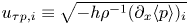 $u_{\tau p,i} \equiv \sqrt {-h\rho ^{-1}(\partial _x \langle p \rangle )_i}$ (the friction velocity based on the pressure gradient forcing before acceleration),
 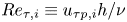 $Re_{\tau,i} \equiv u_{\tau p,i} h/\nu$ is the initial friction Reynolds number, and
  $Re_m \equiv U_m2h/\nu$ is the bulk mean Reynolds number, with
  $U_m$ being the bulk mean velocity (averaged over the entire channel). Each term on the right-hand side of (4.1) is modelled since they are not known a priori. A benefit of this approach is that the pressure gradient remains unaffected by the LES wall model, and the LES have the exact same pressure gradient forcing as used in the DNS of Jung & Kim (Reference Jung and Kim2017). If
  $t^* = 0$ marks the beginning of the acceleration, then
  $Re_m$ is set according to
 $$\begin{gather} Re_m(t^*) = Re_{m,i}, \quad t^* < 0, \end{gather}$$
 $$\begin{gather}Re_m(t^*) = Re_{m,i} + \frac{t^*}{T^*}\, ( Re_{m,f} - Re_{m,i} ), \quad 0 \leq t^* < T^*, \end{gather}$$
 $$\begin{gather}Re_m(t^*) = Re_{m,f}, \quad t^* \geq T^*, \end{gather}$$
where the initial and final bulk mean Reynolds numbers  $Re_{m,i}$ and
  $Re_{m,f}$, respectively, are estimated to give the correct initial and final friction Reynolds numbers. For all simulations considered in this study, the initial and final friction Reynolds numbers are
  $Re_{\tau,i}=180$ and
  $Re_{\tau,f}=395$ to match those of Jung & Kim (Reference Jung and Kim2017). Since these are low Reynolds numbers, following Jung & Kim (Reference Jung and Kim2017) we use the empirical relationship given by Dean (Reference Dean1978) to relate the bulk mean Reynolds number to the friction Reynolds number:
 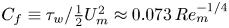 $C_f \equiv \tau _w/\frac 12 U_m^2 \approx 0.073\,Re_m^{-1/4}$. To obtain
  $Re_{m,i}$ and
  $Re_{m,f}$ as functions of
  $Re_{\tau,i}$ and
  $Re_{\tau,f}$, respectively, we use
 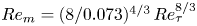 $Re_m = (8/0.073)^{4/3}\,Re_\tau ^{8/3}$. Then once
  $Re_m(t)$ has been obtained from (4.2)–(4.4), we use the inverse relation
  $Re_\tau = (0.073/8)^{1/2}\,Re_m^{3/8}$ to substitute
  $Re_\tau (t)$ into (4.1) to obtain the pressure gradient forcing.
Table 2 shows the acceleration rates considered and their corresponding flow regimes. The flow regime classification is based on the work of Jung & Kim (Reference Jung and Kim2017) and the trends observed for the skin friction. A flow is considered ‘transitional’ if laminar-like behaviour is observed initially (e.g. through the skin friction) that breaks down into a new turbulent state as turbulent spots form. A flow is considered ‘quasi-steady’ if the skin friction does not deviate far from its steady value at a given flow rate (i.e. it agrees with ‘Dean's correlation’ specified above). The ‘intermediate’ flow does not exhibit transitional characteristics, yet its skin friction differs enough from its steady value that it cannot be labelled quasi-steady.
Table 2. The acceleration/ramp rates simulated, and the flow regime classification. For comparison, the relevant wall-modelling time scales are  $T_s^* = 2.20$,
  $t_\nu ^*/h = 0.80$ and
  $T_\varDelta ^* = 1.22$, where the time scales are computed before the flow is accelerated (i.e.
  $t^* \leq 0$).

Large-eddy simulations were performed with the MTS wall model and compared against LES with the EQWM. The domain length, resolution and other simulation details are the same as the pulsatile channel flow, specified in § 3. Again, a constant CFL 0.05 was used, which gives an initial time step size  $\delta t^* \approx 4.6\times 10^{-4}$, and a final time step size (long after the acceleration)
  $\delta t^* \approx 1.9\times 10^{-4}$. Note that the time step size decreases as the flow accelerates, to achieve a constant CFL. This time step size is several orders of magnitude smaller than the fastest acceleration rate, thus ensuring that all dynamics are well resolved temporally.
Figure 17 shows time signals of the imposed pressure gradient forcing and the resulting bulk mean Reynolds numbers for each of the acceleration rates. The pressure gradient forcing is designed to be the same between the LES and the DNS of Jung & Kim (Reference Jung and Kim2017), which is observed in figure 17(a). However, the mean Reynolds number is not controlled directly, so there can be discrepancies between the LES and DNS, which we see in figure 17(b). The acceleration rates match well between the DNS and the LES with largest deviations occurring for the slowest acceleration rate ( $T^*=10$) at the end of the acceleration period. This is caused by a combination of factors, with the primary contributors being the performance of the wall model and the SGS model.

Figure 17. Time signals of (a) the pressure gradient forcing, and (b) the mean Reynolds number ( $Re_m = 2 h U_m/\nu$) divided by the initial mean Reynolds number,
  $Re_{m,i}$, for different acceleration ramp rates. Ramp rates
  $T^* = 0.1, 1.0, 3.0, 5.0, 10.0$ correspond to black, blue, red, green and magenta lines, respectively. Line types for the DNS of Jung & Kim (Reference Jung and Kim2017), LES with the MTS wall model, and LES with the EQWM are dashed, solid and dashed-dot, respectively.
Figure 18 shows the mean velocity (figures 18a,c) and mean Reynolds stresses (figures 18b,d) before the acceleration (figures 18a,b) and long after the acceleration once the flow has reached its new steady-state (figures 18c,d). The LES and DNS agree reasonably well, with overall trends similar to those observed and discussed for the time-averaged profiles of pulsating channel flow (figure 5). Note that the slight overprediction of the velocity near the centre of the channel causes the overprediction of the mean Reynolds number after the acceleration period seen in figure 17(b).

Figure 18. The mean velocity profiles and Reynolds stresses (a,b) before acceleration and (c,d) after acceleration, once the flow has achieved its new steady state. Dashed lines correspond to the DNS of Moser, Kim & Mansour (Reference Moser, Kim and Mansour1999), circles with solid connecting lines correspond to LES with the MTS wall model, and plus signs with dashed-dot connecting lines correspond to LES with the EQWM. In (b,d),  $\langle u'u' \rangle$,
  $\langle v'v' \rangle$,
  $\langle w'w' \rangle$ and
  $\langle u'v' \rangle$ are shown with blue, red, green and black lines, respectively.
Time signals of the planar-averaged wall stress for each of the acceleration rates considered are shown in figures 19 and 20. We first show the results in terms of the skin friction coefficient  $C_f \equiv 2\tau _w/U_m^2$ in figure 19, in order to highlight the evolution during what is often termed a ‘turbulent to turbulent transition’. The acceleration process is marked by an initial fast increase in the skin friction, where a laminar Stokes layer develops; the skin friction then decays until the transition time, where (in the DNS) turbulent streaks would start developing and ultimately increase the skin friction to a new turbulent state at a higher Reynolds number. For example, He et al. (Reference He, Ariyaratne and Vardy2011) identify three acceleration stages for the wall stress with the following characteristics: (1) the turbulence remains ‘frozen’ and the wall stress is governed by a laminar solution; (2) the wall stress increases rapidly, with many signatures of a transition-like process; (3) the wall stress approaches its quasi-steady value asymptotically. Across each of these stages, the velocity deviation from its initial value (ensemble-averaged) is governed by the equation
 \begin{equation} \frac{\partial \langle u \rangle^\wedge}{\partial t} ={-}\frac{1}{\rho}\,\frac{\partial \langle p \rangle^\wedge}{\partial x} + \nu\, \frac{\partial^2 \langle u \rangle^\wedge}{\partial y^2} - \frac{\partial \langle u'v' \rangle^\wedge}{\partial y},\end{equation}
where angled brackets represents ensemble averaging, and 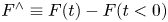 $F^\wedge \equiv F(t) - F(t<0)$ (for any variable
  $F$) indicates the change in a variable from its initial value before the acceleration. Typically, the Reynolds shear stress deviation is neglected during the first stage because the turbulence is assumed to be ‘frozen’ (He et al. Reference He, Ariyaratne and Vardy2011). These arguments lead to a laminar solution to (4.5) (Sundstrom & Cervantes Reference Sundstrom and Cervantes2018c):
 \begin{equation} \langle u_{lam} \rangle^\wedge = U_m \left[ 1 - (1+2\eta^2)\,\textrm{erfc}(\eta) + \frac{2}{\sqrt{\rm \pi}}\,\eta\,\textrm{e}^{-\eta^2} \right], \quad \textrm{where} \ \eta = \frac{y}{\sqrt{4\nu t}}, \end{equation}
which has the corresponding wall stress
 \begin{equation} \langle \tau_{w,lam} \rangle^\wedge = 2 \frac{{\rm d}U_m}{{\rm d}t} \sqrt{\frac{\nu t}{\rm \pi}}.\end{equation}
The thin dotted line in figure 19 shows the laminar analytical solution during this initial acceleration stage (shifted to have initial wall stress  $u_{\tau p,i}^2$). The DNS of Jung & Kim (Reference Jung and Kim2017) are shown with the thick dashed line. All acceleration rates have a brief period where DNS wall stress closely follows the laminar solution. However, for
  $T^*=0.1$ and
  $T^*=1$, the laminar solution persists longer (relative to the acceleration rate), and there is a distinctive time where the skin friction increases quickly, departing from this laminar state. This is a feature of stage 2, and is indicative of a transition-like process occurring. Jung & Kim (Reference Jung and Kim2017) identified these two acceleration rates as having a bypass-like transition. The rest of the acceleration rates are in a state of quasi-equilibrium where the wall stress does not differ far from its steady value at the instantaneous Reynolds number.

Figure 19. Time signals of the skin friction coefficient for different acceleration ramp rates. Ramp rates  $T^* = 0.1, 1.0, 3.0, 5.0, 10.0$ correspond to plots (a–e), respectively. The curves compared are the DNS of Weng et al. (Reference Weng, Boij and Hanifi2016) (thick dashed black line), LES with the EQWM (thick dashed-dot grey line), and LES with the MTS wall model (thick solid black line). The thin black dotted line is the laminar solution given by (4.7).

Figure 20. Time signals of the wall stress for different acceleration ramp rates. Ramp rates  $T^* = 0.1, 1.0, 3.0, 5.0, 10.0$ correspond to plots (a–e), respectively. The curves compared are the DNS of Weng et al. (Reference Weng, Boij and Hanifi2016) (thick dashed black line) and the LES with the MTS wall model (thick solid black line), with LaRTE (thick blue line), lamNEQ (thick red line) and turbNEQ (thick green line) components.
For the slowest acceleration case considered ( $T^*=10$), the MTS wall model and the EQWM show little difference between them over the entirety of the acceleration. This trend is expected since the flow is in a state of quasi-equilibrium, and equilibrium assumptions made by the EQWM are a good approximation. Note that both LES skin frictions differ from the DNS long after the acceleration because of the overpredicted velocity in the wake region as seen in figure 18(c). For the faster acceleration rates, the EQWM performs very poorly relative to the DNS. The EQWM is unable to capture the quick increase in the skin friction caused by the developing laminar Stokes layer. The EQWM also overpredicts the skin friction once the flow starts transitioning to its new turbulent state. During this time, the EQWM incorrectly attributes the increase in velocity to an increase in the wall stress. This undesired effect justifies the use of a velocity correction in the equilibrium closure for the MTS wall model, as introduced in § 2.1.
The MTS wall model, on the other hand, does quite well over each of the acceleration rates considered. It is able to capture the wide range of flow features, from the rapid increase in  $C_f$ initially, to the transition between turbulent states. Figure 20 shows the different contributions to the MTS wall stress so we may see clearly how each component behaves during the different stages of the flow. For all of the acceleration rates, the lamNEQ wall model is dominant when the flow first accelerates. This response allows the MTS wall model to capture the sharp initial increase in the wall stress, which the EQWM is unable to do. Conversely, the LaRTE wall model has a delayed response to the acceleration because of its inherent relaxation dynamics. Without the velocity correction, however, the LaRTE model responds too quickly, causing the wall stress to be overpredicted initially. Also as expected, after the flow has accelerated and approaches its new steady state, the LaRTE model is the primary contributor to the wall stress. In between these two extremes (after the lamNEQ contribution decays, but before the LaRTE model responds), the turbNEQ response is the most prominent. This also happens to be the time when the turbulent-to-turbulent transition occurs. Figures 20(a) and 20(b) show that the turbNEQ model helps to speed up the wall-stress response during this transition stage.
Further insights can be obtained by focusing on the relationship between the LES velocity at the wall-model point and the wall-stress evolution and fluctuations. According to the turbNEQ model (2.20) and (2.22), an increase in  $\tau _{wx}'$ means that the LES velocity is increasing faster than the quasi-equilibrium velocity obtained from LaRTE, thus leading to a velocity deviation
  $u_\varDelta '$ (see figure 21 for time signals of this velocity as well as other model contributions to the LES velocity). For channel flow with a constant pressure gradient, this velocity deviation may be explained by turbulent fluctuations. However, for linearly accelerating channel flow, this velocity deviation has a non-zero average, which can be explained as follows. As the flow accelerates, the initial growth in
  $U_{LES}$ is accounted for by the laminar contribution
  $u_\varDelta ''$, and the turbulent contribution
  $u_\varDelta '$ is small. However, near the flow transition time, the laminar Stokes layer decays as it interacts with the ‘outside’ turbulence, and there is no change in the pressure gradient to drive its growth. This occurs at approximately the time
  $t=t_\nu$ since this time scale is defined as the time for a Stokes layer to grow from the wall to the edge of the laminar viscous sublayer. After this time, there is a difference between the turbulent state away from the wall and near the wall. In DNS studies, this leads to the generation of near-wall streaks and a breakdown to a new turbulent state (He & Seddighi Reference He and Seddighi2013, Reference He and Seddighi2015). In LES with the MTS wall model, this is measured through
  $u_\varDelta '$, and the turbNEQ model attempts to account for the expected increase in the wall stress during transition. In practice, the turbNEQ model responds less quickly than is desirable, as seen by the difference between the DNS and LES curves after transition in figure 20. A possible explanation is that the breakdown to turbulence caused by near-wall streak instabilities is a rapid phenomenon (Hack & Zaki Reference Hack and Zaki2014) that is not detected by the first LES velocity point, which is too far from the wall. The turbNEQ model relies solely on LES velocity information and therefore cannot account for this subtle effect whose modelling requires more detailed future efforts.

Figure 21. Time signals at a representative single point  $(x,y,z)=(L_x/2,\varDelta,L_z/2)$ of the different modelling components of the LES velocity for several acceleration ramp rates. Ramp rates
  $T^* = 0.1, 1.0, 3.0, 5.0, 10.0$ correspond to plots (a–e), respectively. The different lines correspond to
  $U_{LES}$,
  $u_\tau f(\varDelta ^+)$,
  $u_\varDelta '$ and
  $u_\varDelta ''$, shown in grey, blue, green and red, respectively.
Single-point time signals (no planar averaging) of the different modelled components of the LES velocity are shown in figure 21. The LES velocity ( $U_{LES}$ shown in grey) is decomposed according to (2.20), with LaRTE (
 $u_\tau f(\varDelta ^+)$, shown in blue), lamNEQ (
 $u_\varDelta '$, shown in red) and turbNEQ (
 $u_\varDelta ''$, shown in green) contributions. It is clear from the figure that the LaRTE portion effectively filters out the large LES velocity fluctuations due to the relaxation dynamics of LaRTE. It also captures the mean value before and after the linear acceleration. The lamNEQ portion captures the initial linear behaviour of the velocity as soon as the flow accelerates. The turbNEQ contribution is twofold. On the one hand, it is responsible for capturing the majority of the LES velocity fluctuations. On the other hand, it captures the behaviour of the velocity in response to transition, as discussed previously. Figure 21 demonstrates the usefulness of decomposing a complicated flow into its constitutive parts, as is possible with the MTS wall model.
Figure 22 shows time signals of the (planar-averaged) velocity perturbation at different heights for a fast acceleration case ( $T^*=0.1$) and a slow acceleration case (
 $T^*=5$). For the fast acceleration case, the LES for both wall models gives the correct linear trend during the accelerating phase. However, after the acceleration is over, the LES predicts a decrease in the velocity perturbation too soon (with the exception of the channel centreline), with the EQWM generally giving a larger drop in the velocity perturbation than the MTS wall model, the latter therefore being closer to the DNS data. For the slow acceleration case, the LES and the DNS agree well over all times. This is expected since the flow is in a state of quasi-equilibrium and thus both wall models yield similar mean wall stresses.

Figure 22. Time signals of the velocity perturbation (from the initial condition) at several heights for (a)  $T^*=0.1$ and (b)
  $T^*=5.0$. From light to dark lines, the heights correspond to
  $y/h = 0.167, 0.5, 0.967$, which are the third, eighth and centreline LES grid points, respectively. The DNS (from Jung & Kim Reference Jung and Kim2017), the LES with the MTS wall model, and the LES with the EQWM correspond to dashed lines with filled circles, solid lines, and dashed-dot lines, respectively. The circles correspond to the sample times given for the DNS.
5. The MTS wall model in the limit of instantaneous relaxation
A possible variant of the MTS wall model is now explored by considering the limit of a vanishingly small relaxation time scale, i.e.  $T_s \to 0$. In that limit, the friction velocity from LaRTE is equal to its equilibrium value (i.e.
  ${\boldsymbol u}_\tau = \bar {\boldsymbol {\tau }}_w^{eq}/(\bar {\tau }_w^{eq})^{1/2}$, with the corresponding wall stress
  $u_\tau {\boldsymbol u}_\tau = \bar {\boldsymbol {\tau }}_w^{eq}$), and the quasi-equilibrium velocity becomes
  $\bar {\boldsymbol u}_\varDelta = {\boldsymbol u}_\tau \,f(\varDelta ^+)$, since
  ${\boldsymbol u}_\tau$ is obtained from the equilibrium model that uses
  $\bar {\boldsymbol u}_\varDelta$ as input velocity. Therefore, according to (2.20),
  $\boldsymbol {u}'_\varDelta = 0$ and the turbulent turbNEQ portion is subsumed into the equilibrium wall-model contribution. The total wall stress for the MTS wall model in the limit
  $T_s \to 0$ is then simply
 \begin{equation} \boldsymbol{\tau}_w = \bar{\boldsymbol{\tau}}_w^{eq} + \boldsymbol{\tau}_{w}'',\end{equation}
where  $\bar {\boldsymbol {\tau }}_w^{eq}$ is evaluated according to the fit from (2.13), and
  $\boldsymbol {\tau }_{w}''$ is governed by (2.18). The MTS wall model in the limit of instantaneous relaxation, governed by (5.1), is referred to as the equilibrium MTS (EQMTS) wall model. It is important to note that the quasi-equilibrium velocity input still contains the velocity correction to the LES velocity ((2.14) and (2.15)) to account for changes in the LES velocity caused by the laminar Stokes layer. For succinctness, the equilibrium model component
  $\bar {\boldsymbol {\tau }}_w^{eq}$ with a corrected velocity input is referred to as the ‘corrected equilibrium’ model.
We now apply this model to pulsating and linearly accelerating channel flow. Representative resulting stress evolution plots are shown in figures 23–25. For pulsating channel flow, the EQMTS wall model is nearly identical to the EQWM for the two lowest frequencies ( $\omega _f^+ = 0.001, 0.003$). For low frequencies, the lamNEQ contribution is relatively small, meaning that the corrected equilibrium wall stress is dominant. Additionally, while
  $T_f \gg T_\varDelta$, the velocity correction has a negligible impact and the corrected equilibrium wall model thus behaves similarly to the standard EQWM (e.g. see figure 24(a) where the corrected equilibrium wall-stress component and EQWM curves are nearly indistinguishable). These two effects cause the EQMTS wall model to behave similarly to the EQWM for low frequencies where performance is good.

Figure 23. Single-period time evolution of the periodic streamwise wall stress  $\tilde {\tau }_{wx}$ for several forcing frequencies,
  $\omega _f^+=0.001, 0.003, 0.006, 0.01, 0.02, 0.04$ (plots (a–f), respectively). Line types correspond to LES using the MTS wall model (thick solid black), LES using the EQWM (thick dashed-dot grey), LES using the equilibrium MTS wall model (thick dotted black) and DNS from Weng et al. (Reference Weng, Boij and Hanifi2016) (thick dashed black). The phase within the cycle is based on the imposed forcing frequency.
Most evident in figure 23(d), the total EQMTS wall stress is not sinusoidal. From figure 24, we see that this is caused by the corrected equilibrium model component, which becomes non-sinusoidal as frequency is increased. This must be caused by the velocity correction since this is the only difference between the corrected equilibrium and EQWM models. The model (2.14) shows that  $\boldsymbol {u}_\varDelta ''$ evolves at time scale
  $T_\varDelta$. When subtracted from the LES velocity (which evolves at the forcing period
  $T_f$), the quasi-equilibrium velocity input becomes distorted and non-sinusoidal if
  $T_f$ and
  $T_\varDelta$ are of similar order. This occurs in the intermediate- and high-frequency regimes.
For high frequencies, the EQMTS wall model behaves similar to the regular MTS wall model. This is primarily because the lamNEQ model is dominant here, which is shared between the two models and therefore any differences between the corrected equilibrium model and the LaRTE+turbNEQ stresses (figure 24c) are small relative to the total wall stress. At high frequencies ( $\omega _f^+ \geq 0.04$), the velocity correction effectively filters out the corresponding high frequency content of the LES velocity, which causes the equilibrium portion of the equilibrium MTS wall model to respond slowly, similarly to the LaRTE model. Without the velocity correction, the total wall stress for the EQMTS wall model is simply the lamNEQ wall stress plus the EQWM wall stress. This leads to an overprediction of the total wall stress, thus showing the necessity of the velocity correction for non-equilibrium flows.

Figure 24. Single-period time evolution of the periodic streamwise wall stress  $\tilde {\tau }_{wx}$ for low, intermediate and high forcing frequencies,
  $\omega _f^+=0.001, 0.006, 0.04$ (plots (a–c), respectively). Curves shown include the corrected equilibrium component of the EQMTS wall model (dotted blue), the EQWM wall stress (dashed-dot grey), and the LaRTE+turbNEQ wall stresses (solid cyan). The phase within the cycle is based on the imposed forcing frequency.

Figure 25. Time signals of the skin friction coefficient for different acceleration ramp rates. Ramp rates  $T^* = 0.1, 1.0, 3.0, 5.0, 10.0$ correspond to plots (a–e), respectively. The curves compared are the DNS of Weng et al. (Reference Weng, Boij and Hanifi2016) (thick dashed black line), LES with the EQWM (thick dashed-dot grey line), LES with the EQMTS wall model (thick dotted black line), and LES with the MTS wall model (thick solid black line). The thin black dotted line is the laminar solution given by (4.7).
For linearly accelerating channel flow, the EQMTS wall model is able to achieve some of the same trends in the skin friction as the full MTS wall model (e.g. the sharp increase in the skin friction initially), although it tends to overpredict the skin friction after the laminar stage of the acceleration. The velocity correction allows the EQMTS model to have a delayed response to changes in the pressure gradient so that the lamNEQ model can capture the non-equilibrium response to fast changes in the pressure gradient. However, the velocity correction time scale  $T_\varDelta$ appears to not be long enough for the EQMTS wall model to give the correct wall stress since the skin friction begins to increase too early for all of the acceleration rates shown in figure 25. In fact, the EQMTS wall stress even exceeds the EQWM wall stress during portions of the flow acceleration for the slow acceleration cases. This must be caused by the slow decay of the lamNEQ wall stress since the corrected equilibrium wall stress
  $\bar {\boldsymbol {\tau }}_w^{eq}$ can never be greater than the EQWM wall stress (since it is essentially just a delayed version of it).
We now comment briefly on the differences in computational cost between the wall models considered. For all wall-modelled LES considered here, the computational cost remains insignificant compared to wall-resolved LES because the wall models do not require solving equations on a fine, near-wall mesh (see e.g. Choi & Moin (Reference Choi and Moin2012) and Yang & Griffin (Reference Yang and Griffin2021) for more details). For pulsatile channel flow, the average percentage of time spent in the wall-model function call (over the total time spent per time step) was measured to be 18.973 % for the MTS wall model, 16.373 % for the EQMTS wall model, and 3.390 % for the EQWM. Similar percentages were found for the linearly accelerating channel flow. The  $\sim$3 % of time spent for the EQWM is consistent with expectations since 30 grid points were used in the wall-normal direction, and wall model computations are done over a single horizontal plane. The additional
  $\sim$15 % of time spent for the MTS and EQMTS wall models is a direct result of the additional 48 exponential terms (per point on the horizontal wall-modelling plane) needed for the lamNEQ model. This increase in cost is expected since
  $N_{exp}$ times more computations were used for the lamNEQ model. However, it is clear from the present results that the lamNEQ model plays a critical role in properly modelling the wall stress in instances of high non-equilibrium, therefore no effort was made to reduce
  $N_{exp}$ to decrease the computational cost. It is possible that further gains in efficiency could be made by reducing
  $N_{exp}$ following a careful study of loss of accuracy versus computational efficiency. In this work, we opted to keep the model highly accurate since the overall cost increase was relatively small. Finally, the minor difference in cost between the MTS and EQMTS wall models shows that the additional complexity of the LaRTE model does not equate with a significant increase in computational time.
Overall, the EQMTS wall model is able to capture several of the important features in non-equilibrium flows (since the lamNEQ model captures the majority of these dynamics) while maintaining some of the simplicity of the EQWM. While the full MTS model agrees somewhat better with the DNS for the majority of the non-equilibrium flows tested, the EQMTS wall model can be considered as a simpler alternative since it does not require the solution of the LaRTE friction-velocity transport equation.
6. Conclusions
A multi-time-scale (MTS) wall model for large-eddy simulations has been developed and applied to a wide variety of flows, from quasi-equilibrium to non-equilibrium conditions. The MTS wall model consists of LaRTE, lamNEQ and turbNEQ components that allow the wall model to capture the full range of time scales necessary to model non-equilibrium flows. Figure 1 presents the various length and time scales included in the MTS wall model. The LaRTE+lamNEQ model (originally introduced in Fowler et al. Reference Fowler, Zaki and Meneveau2022) has been augmented to represent additional physical effects not included before. For the LaRTE model, this includes a newly added ‘velocity correction’ to the LES velocity input to the equilibrium closure, and inclusion of the full pressure gradient term in the closure (both discussed in § 2.1). The velocity correction allows for a more accurate prediction of  $\bar {\boldsymbol {\tau }}_\varDelta$ when using an equilibrium closure. And to represent the contributions from unresolved turbulent eddies, we introduced the turbNEQ term, which models the wall-stress response to velocity fluctuations around their quasi-equilibrium value (see (2.20)). It is worthwhile pointing out that the quasi-equilibrium portion of the MTS model bears resemblance to behaviour of slow, large-scale outer boundary layer motions that have been observed to cause amplitude modulation of near-wall, small-scale turbulence (Mathis et al. Reference Mathis, Hutchins and Marusic2009). Amplitude modulation is a phenomenon that has received considerable attention over the past decade (Marusic & Monty Reference Marusic and Monty2019). In future work, it would be of interest to explore the relationship between the LaRTE inherent time scale
  $T_s$ and the characteristic time scale of the modulating motions identified in the work of Mathis et al. (Reference Mathis, Hutchins and Marusic2009).
The MTS wall model was then applied to two distinct non-equilibrium flows, namely pulsating channel flow in § 3, and linearly accelerating channel flow in § 4. For pulsating channel flow, the forcing frequency was varied to achieve conditions ranging from quasi-equilibrium to non-equilibrium. As expected, for low frequencies, the MTS wall model and EQWM are very similar and agree well with the DNS of Weng et al. (Reference Weng, Boij and Hanifi2016). However, as the frequency is increased, the EQWM departs progressively from the DNS results, whereas the MTS wall model displays good agreement with the DNS. Time signals of the different components of the MTS wall model show that the LaRTE, turbNEQ and lamNEQ wall stresses are most dominant for low, intermediate and high frequencies, respectively. This is consistent with the length and time scale schematic of figure 1. Amplitude and phase plots of the periodic velocity show little difference between the MTS wall and the EQWM over all of the frequencies tested. However, amplitude and phase plots of the periodic Reynolds stresses show a dependency on the wall model, with complicated trends that have so far eluded any straightforward explanation.
For linearly accelerating flow, the acceleration rate was varied from very rapidly accelerating, non-equilibrium conditions (where bypass transition-like behaviour is observed in the DNS) to slowly accelerating, quasi-steady conditions. The MTS wall model performs significantly better than the EQWM for the majority of the acceleration rates (except for the slowest  $T^*=10$ case, where performance is similar). Time signals of the various constitutive components of the MTS wall model show that different terms are dominant during each stage of the flow acceleration. During the laminar, transition and quasi-steady stages, the lamNEQ, turbNEQ and LaRTE components, respectively, provide the largest contribution to the wall-stress response to acceleration. These trends are again consistent with the situation illustrated in figure 1.
Finally, motivated by practical considerations, we explore the MTS wall model in the limit of instantaneous relaxation called the equilibrium MTS wall model (EQMTS). This approach keeps some of the simplicity of the traditional EQWM while maintaining most of the accuracy of the full MTS wall model during non-equilibrium conditions. It leverages the observation that the EQWM with velocity correction behaves similarly to the LaRTE+turbNEQ models. For both pulsating and linearly accelerating channel flow, the EQMTS wall model captures the majority of the mean wall-stress time evolution. The most noticeable differences between EQMTS and the full MTS wall models include non-sinusoidal behaviour during intermediate forcing frequencies, and an overprediction of the skin friction during the transition stage for the two fastest flow accelerations considered.
In Appendix A, the equilibrium/stationary channel flow and SSPG test cases from Fowler et al. (Reference Fowler, Zaki and Meneveau2022) are repeated for the MTS wall model. The streamwise wall-stress probability density functions for the equilibrium channel flow actually improve relative to the original LaRTE+lamNEQ wall model. This is due primarily to the turbNEQ model, which dominates wall-stress fluctuations for the MTS wall model. The spanwise wall-stress variance is overpredicted, however, which appears to be related to the overprediction of the spanwise resolved velocity fluctuation variance in the LES due to the SGS closure, as mentioned in § 3. For the SSPG flow, the MTS wall model shows good agreement with the DNS for the spanwise component of the wall stress, similar to what was seen in the LaRTE+lamNEQ model of Fowler et al. (Reference Fowler, Zaki and Meneveau2022). The streamwise wall-stress component, however, shows an increased delayed response to the SSPG, and still cannot predict the short drop in  $\tau _{wx}$ caused by the scrambling of momentum-carrying turbulent structures, which would require further modelling.
Future work will focus on developing and testing the MTS wall model for flows with non-equilibrium in space instead of the temporal non-equilibrium conditions considered in this work. The shear stress closure for  $\bar {\boldsymbol {\tau }}_\varDelta$ already contains weak effects of non-equilibrium since the fit
  $Re_{\tau \varDelta }^{pres}$ incorporates the LES pressure gradient information in estimating the local shear stress. However, further testing is needed to ascertain the performance of the MTS model for spatial non-equilibrium where ‘history effects’ are significant, or cases with separation where the wall stress is zero locally. Due to the Lagrangian nature of the relaxation time delay in the LaRTE portion of the MTS model, there is nothing structurally preventing us from simulating flows with spatial non-equilibrium. However, the non-equilibrium portions of the MTS model, especially the laminar model, may be different from the temporal models developed here. More work is needed to examine such modelling aspects.
Supplementary material
Computational Notebook files are available as supplementary material at https://doi.org/10.1017/jfm.2023.585 and online at https://cambridge.org/S0022112023005852/JFM-Notebooks.
Funding
This work is supported by a grant from the Office of Naval Research (grant no. N00014-21-1-2162, Dr P. Chang is program manager).
Declaration of interests
The authors report no conflict of interest.
Appendix A. Revisiting wall-stress probability density functions and SSPG flow
The wall-stress probability density functions (PDFs) in equilibrium channel flow, as well as the sudden spanwise pressure gradient (SSPG) flow studied in Fowler et al. (Reference Fowler, Zaki and Meneveau2022) (based on the DNS of Lozano-Durán et al. Reference Lozano-Durán, Giometto, Park and Moin2020), are revisited here, in order to discuss how the addition of the non-equilibrium turbulent model (and the other model changes) affects the results. The same grid and subgrid scale model as in the original SSPG test in Fowler et al. (Reference Fowler, Zaki and Meneveau2022) are used. The first grid point is used for the wall model height. Major differences between LaRTE+lamNEQ and the newly proposed MTS wall model include: (1) treatment of the pressure gradient in the LaRTE relaxation term; (2) introducing velocity correction to the LES velocity input for computing the equilibrium stress; and (3) addition of the turbNEQ wall model.
First, we consider equilibrium channel flow at  $Re_\tau = 1000$ and 5200, repeating figure 10 of Fowler et al. (Reference Fowler, Zaki and Meneveau2022) but using the MTS model. Results are shown in figure 26 and are compared with DNS (dashed black line). Compared to the model version used in Fowler et al. (Reference Fowler, Zaki and Meneveau2022), it is evident that the addition of the turbNEQ portion of the model in the MTS approach yields very realistic PDFs of the streamwise component of the wall stress as compared to filtered DNS, but overestimates the level of variability of the spanwise wall-stress component. A simple explanation is that the current LES overpredicts the spanwise velocity fluctuations in the near-wall region, as can be seen in figures 5(b) and 18(b,d) for low Reynolds numbers, and figure 5 in Fowler et al. (Reference Fowler, Zaki and Meneveau2022) for high Reynolds numbers. Since the turbNEQ wall stress is proportional to the LES velocity fluctuations at the wall-model height, this leads directly to overpredicted wall-stress fluctuations.

Figure 26. PDFs for  $\tau _{wx}$ and
  $\tau _{wz}$, for (a,b)
  $Re_\tau = 1000$, and (c,d)
  $Re_\tau = 5200$. The PDF curves correspond to the filtered DNS (dashed black lines), the LaRTE model (blue lines), the lamNEQ model (red lines), the turbNEQ term (green lines) and the MTS model (solid black lines). DNS data are obtained from the Johns Hopkins Turbulence Database (Graham et al. Reference Graham2016; JHTDB 2021). The DNS PDFs are obtained from the Gaussian filtered wall stress where the filtering size is the same as the LES mesh size in the horizontal directions.
In order to help to visualize the response of the wall stress to velocity fluctuations in the LES using the MTS wall model, in figure 27 we show the superposition of the various model terms. An animation can be rotated interactively to improve understanding of the model.

Figure 27. Assumed velocity profile below the wall-model grid point for the MTS wall-model approach. For an interactive animation of this sketch, see https://www.cambridge.org/S0022112023005852/JFM-Notebooks/files/Figure-27/steady_channel_flow_wm_velocity_profiles.html. (To play the animation, select ‘Controls’ and ‘Play loop’ on the K3D panel.) The source code that generated the animation can be found at https://www.cambridge.org/S0022112023005852/JFM-Notebooks/files/Figure-27/steady_channel_flow_wm_velocity_profiles.ipynb. Line colours for the total modelled velocity and its LaRTE, lamNEQ and turbNEQ components are black, blue, red and green, respectively. Thin coloured lines are the model's streamwise and spanwise velocity profiles.
Next, we examine the SSPG flow. The evolution of the predicted spatially averaged mean wall stress is shown in figure 28. For the streamwise wall stress, the MTS wall model has a slightly more delayed response compared with the LaRTE+lamNEQ results in Fowler et al. (Reference Fowler, Zaki and Meneveau2022) (results not shown here). This delayed response is likely caused by differences (1) and (2) stated above. However, we deem this behaviour acceptable since these differences to the DNS are small relative to the total wall-stress change after the SSPG is introduced. The spanwise wall stress, shown in figure 28(b), is very similar to that shown in Fowler et al. (Reference Fowler, Zaki and Meneveau2022) despite the significantly slower response of the LaRTE model shown by the blue curve. For the spanwise direction, the LaRTE model is slower, due primarily to the treatment of the pressure gradient in the relaxation term ( ${\boldsymbol \nabla }_h \bar {p}$ in (2.5)). In both Fowler et al. (Reference Fowler, Zaki and Meneveau2022) and the present work, the quasi-equilibrium pressure gradient is evaluated as the filtered LES pressure gradient with the filtering time scale
  $t_\nu$. However, in Fowler et al. (Reference Fowler, Zaki and Meneveau2022), part of this pressure gradient is brought into the equilibrium stress closure (see (2.13)) and part of it is left in the relaxation term as a ‘band-pass filtered pressure gradient’. In the present work, all of
  ${\boldsymbol \nabla }_h \bar {p}$ is brought into the equilibrium stress closure, therefore there is no leftover relaxation term. When changes in the pressure gradient are large (as is the case with the SSPG flow), this term can become quite significant and speeds up the response of the LaRTE model. We chose to keep all of the quasi-equilibrium pressure gradient in the equilibrium stress closure since the LaRTE model now truly relaxes to its ‘equilibrium stress’ while the turbNEQ model makes up for the delayed response of the LaRTE model.

Figure 28. (a) Streamwise and (b) spanwise wall stress after a suddenly applied spanwise pressure gradient. Line types correspond to the DNS of Lozano-Durán et al. (Reference Lozano-Durán, Giometto, Park and Moin2020) (thick dashed black lines), LES with the EQWM (dashed-dot grey lines), and the total wall stress for LES with the MTS wall model (solid black lines). In (b), wall stresses for the LaRTE, lamNEQ and turbNEQ components of the MTS wall model are shown with blue, red and green lines, respectively. The thin dotted line in (b) corresponds to the Stokes solution wall stress. Angled brackets represent ensemble averaging over the horizontal plane and over five independent simulations.
The turbNEQ wall model, by design, assumes that a wall stress is generated if the LES velocity (with velocity correction) responds more quickly than the quasi-equilibrium velocity  $\boldsymbol {u}_\tau f(\varDelta ^+)$. The green curve in figure 28(b) shows that initially the difference between these two velocities is small. It then reaches a peak at approximately
  $tu_{\tau p,i}/h=0.5$, subsequently decaying until the flow reaches a new quasi-equilibrium state long after the SSPG is applied. Other wall-stress trends for the LaRTE and lamNEQ models discussed in Fowler et al. (Reference Fowler, Zaki and Meneveau2022) are also observed here (e.g. the fast initial response of the lamNEQ model). Overall, the MTS wall model agrees well with the DNS results, with improvement over the popular EQWM.
Figure 29 shows contour plots of the wall-stress fluctuations for each component of the MTS wall model after the SSPG is applied. Only one time instance,  $tu_{\tau p,i}/h=2.22$, is shown in the figure here; however, the entire time history before and after the SSPG may be viewed using the animation link provided in the figure caption. From the figure, it is clear that the turbNEQ wall model is the primary contributor to wall-stress fluctuations. This is generally true for all conditions from quasi-equilibrium to non-equilibrium. The LaRTE model tends to capture slow large-scale wall-stress fluctuations that appear as elongated turbulent streaks in figures 29(a,b). Similar to what was reported in Fowler et al. (Reference Fowler, Zaki and Meneveau2022), we observe a break-up of the LaRTE wall-stress streaks initially after the SSPG is applied, which then eventually re-align themselves with the mean wall-stress direction as the flow approaches asymptotically its new quasi-equilibrium state. We stress that these streaks are very large, corresponding to the response time
  $T_s$, which is significantly larger than the large-eddy turnover time
  $\varDelta /u_\tau$ (by a factor
  $f(\varDelta ^+)$).

Figure 29. Contour plots of the wall-stress fluctuations (both streamwise and spanwise directions) for each component in the MTS wall model after the SSPG is applied at  $tu_{\tau p,i}/h=+2.22$. These components include (a,b) LaRTE, (c,d) lamNEQ, (e, f) turbNEQ, and (g,h) the total MTS wall stress. The dashed lines in (a,b) represent the total wall-stress angle. Angled brackets represent averaging over the horizontal plane. An animation of the wall-stress evolution before (
 $t<0$) and after (
 $t>0$) the SSPG can be seen at https://www.cambridge.org/S0022112023005852/JFM-Notebooks/files/Figure-29/sspg_ws_contour_animation.html. The corresponding source code can be found at https://www.cambridge.org/S0022112023005852/JFM-Notebooks/files/Figure-29/sspg_ws_contour_animation.ipynb.
For this particular flow, the lamNEQ wall-stress fluctuations are small in magnitude, although with large spatial variability, relative to the turbNEQ wall-stress fluctuations. Generally, the lamNEQ wall-stress fluctuations relative to the turbNEQ fluctuations decrease as Reynolds number increases. This is because  $\boldsymbol {\tau }_w''/u_\tau ^2$ scales with
  $Re_\tau ^{-1/2}$, whereas
  $\boldsymbol {\tau }_w'/u_\tau ^2$ scales with
  $\boldsymbol {u}_\varDelta '/u_\tau$, which increases with Reynolds number. For
  $Re_\tau =1000$, the Reynolds number is large enough such that turbulent velocity fluctuations are the dominant contributors to wall-stress fluctuations.
Appendix B. Alternative derivation of the LaRTE equation
The original derivation of the LaRTE equation in Fowler et al. (Reference Fowler, Zaki and Meneveau2022) focused on the terms along the near-wall streamline direction  ${\boldsymbol s}$. As shown below, a more complete derivation can be done using index notation that brings out an additional term not included in the original derivation. The horizontal momentum equation (2.4) rewritten in index notation is given by
 \begin{align} &\frac{\partial \bar{u}_{si}}{\partial t} + \partial_j(\bar{u}_{si} \bar{u}_{sj}) + \partial_y(\bar{v} \bar{u}_{si}) \nonumber\\ &\quad ={-}\rho^{{-}1}\,\partial_i \bar{p} + \frac{\partial}{\partial y} \left[ (\nu + \nu_T)\,\frac{\partial \bar{u}_{si}}{\partial y}\right] + \partial_j [ (\nu + \nu_T) ( \partial_i \bar{u}_{sj} + \partial_j \bar{u}_{si} ) ], \end{align}
where indices correspond to the horizontal directions, i.e.  $i=1,3$, and the horizontal velocity follows the law of the wall, i.e.
  $\bar {u}_{si} = u_{\tau i}\,f(y^+) = u_\tau s_i\,f(y^+)$. The continuity equation is
 \begin{equation} \partial_i \bar{u}_{si} + \partial_y \bar{v} = \partial_s \bar{u}_s + \bar{u}_s (\partial_i s_i) + \partial_y \bar{v} = 0,\end{equation}
where we have used the relation  $\partial _s = s_i \partial _i$. Equation (B2) can be integrated to obtain the vertical velocity at the wall-model height:
 \begin{equation} \bar{v}(\varDelta) ={-} \int_0^\varDelta \partial_i \bar{u}_{si} \,{{\rm d} y} ={-} \int_0^\varDelta \partial_i (u_\tau s_i f) \,{{\rm d} y} ={-}(\partial_s u_\tau) \varDelta f_\varDelta - u_\tau (\partial_i s_i) \int_0^\varDelta f \,{{\rm d} y},\end{equation}
where  $f_\varDelta \equiv f(\varDelta ^+)$, and the term proportional to
  $\partial _i s_i$ was omitted in Fowler et al. (Reference Fowler, Zaki and Meneveau2022).
Equation (B1) is now integrated vertically from the wall to the wall-model height to obtain the LaRTE equation. The nonlinear advection term is then
 \begin{equation} \int_0^\varDelta [ \partial_j(\bar{u}_{si} \bar{u}_{sj}) + \partial_y (\bar{v} \bar{u}_{si})] \,{{\rm d} y} = \int_0^\varDelta \partial_j(\bar{u}_{si} \bar{u}_{sj}) \,{{\rm d} y} + \bar{v}(\varDelta)\,u_\tau s_i f_\varDelta.\end{equation}
The first term requires expanding, and after some manipulation can be written as
 \begin{equation} \int_0^\varDelta \partial_j (\bar{u}_{si} \bar{u}_{sj}) \,{{\rm d} y} = u_{\tau i} (\partial_s u_\tau)\,\varDelta f_\varDelta^2 + [ u_\tau (\partial_s u_{\tau i}) + u_\tau^2 s_i (\partial_j s_j) ] \int_0^\varDelta f^2 \,{{\rm d} y}.\end{equation}
Substituting (B5) and (B3) into (B4), and dividing by  $\varDelta f_\varDelta$ (the coefficient for the time derivative term), yields for the LaRTE advection term
 \begin{equation} \frac{1}{\varDelta f_\varDelta} \int_0^\varDelta [ \partial_j(\bar{u}_{si} \bar{u}_{sj}) + \partial_y (\bar{v} \bar{u}_{si})] \,{{\rm d} y} = V_{\tau j} (\partial_j u_{\tau i}) - u_\tau f_\varDelta (\partial_j s_j) \left( \frac{\theta_\varDelta}{\varDelta}\right) u_{\tau i},\end{equation}
where  $\boldsymbol {V}_\tau$ is the advection velocity for the friction velocity introduced in § 2.1, and integrals have been rewritten in terms of the cell displacement (
 $\delta _\varDelta ^*$) and momentum (
 $\theta _\varDelta$) thicknesses, also introduced in § 2.1. The complete LaRTE model, without simplifications, is then (returning to Gibbs notation)
 \begin{align} &\frac{\partial {\boldsymbol{u}}_\tau}{\partial t} + {\boldsymbol V}_\tau \boldsymbol{\cdot} \boldsymbol{\nabla}_h {\boldsymbol{u}}_\tau = \frac{1}{T_s} \left[ \frac{1}{u_\tau}\left(-\frac{\varDelta}{\rho}\, \boldsymbol{\nabla}_h \bar{p} + \bar{\boldsymbol{\tau}}_\varDelta \right) - {\boldsymbol u}_\tau\right] + u_\tau\, \frac{\delta^*_\varDelta}{\varDelta}\, \frac{\partial {\boldsymbol s}}{\partial t} \nonumber\\ &\quad + u_\tau f_\varDelta ({\boldsymbol \nabla}_h \boldsymbol{\cdot} \boldsymbol{s}) \left( \frac{\theta_\varDelta}{\varDelta}\right) \boldsymbol{u}_{\tau} + \frac{1}{\varDelta f_\varDelta}\,{\boldsymbol \nabla}_h \boldsymbol{\cdot} \boldsymbol{\mathsf{D}}_\tau, \end{align}
where  $\boldsymbol{\mathsf{D}}_\tau$ is the horizontal diffusion term (vertical integral of the last term in (B1)), discussed in Fowler et al. (Reference Fowler, Zaki and Meneveau2022). The last two terms in (B7) are excluded in numerical implementation of the model due to their expected minor impact on the results (e.g.
  $\theta _\varDelta /\varDelta \lesssim 0.1$) and added complexity in evaluating them numerically.


 Open access