


1. Introduction
Einstein metrics are central in geometry and physics. Being critical for the Einstein–Hilbert functional $\mathcal {EH}:g \mapsto \mathcal {EH}(g)=\int _M \tau _g\,\operatorname {dvol}_g$ subject to a volume constraint, they provide optimal metrics in the sense that the scalar curvature $\tau$
 is more evenly distributed about the manifold. Since the space of scalar curvature invariants of order one is generated by the scalar curvature, in the search of optimal metrics on a given manifold, it is natural to consider other functionals defined by integrating polynomial curvature invariants of higher order. The space of scalar curvature invariants of order two has dimension at most four and it is generated by $\{ \tau ^{2},\, \Vert \rho \Vert ^{2},\, \Vert R \Vert ^{2},\, \Delta \tau \}$
 . In dimension three, the curvature tensor $R$
 is totally determined by the Ricci tensor $\rho$
 and $\| R\|^{2}=2\Vert \rho \Vert ^{2} -\tfrac {1}{2}\tau ^{2}$
 . Thus, the space of quadratic curvature functionals in dimension three is generated by
Hence, every quadratic curvature functional can be expressed as a multiple of $\mathcal {S}$ or $\mathcal {F}_t = \mathcal {T} +t \mathcal {S}$
 , for some $t \in \mathbb {R}$
 .
.
There are many special cases of the functionals $\mathcal {F}_t$ that can be found in the literature. We cite just a few examples. The functional defined by the L$^{2}$
 -norm of the curvature tensor corresponds to $\mathcal {F}_{-1/4}$
 . For $t=-\frac {1}{3}$
 one has the functional defined by the norm of the trace-free Ricci tensor $\rho _0=\rho -\frac {1}{3}\tau g$
 . The norm of the Schouten tensor $S=\rho -\frac {1}{4}\tau g$
 is given by $\| S\|^{2}=\|\rho \|^{2}-\frac {5}{16}\tau ^{2}$
 , thus defining the functional $\mathcal {F}_{-5/16}$
 . The functional corresponding to $t=-\frac {3}{8}$
 is equivalent to the functional $\sigma _2: g \mapsto \int _M \sigma _2(S_g) \operatorname {dvol}_g$
 defined by the second symmetric elementary function of the eigenvalues of the Schouten tensor (see [Reference Gursky and Viaclovsky15]).
Some of these functionals also play a role in relativistic physics. The functional $\mathcal {F}_{-3/8}$ appears in three-dimensional massive gravity, which is a correction to Einstein's theory of gravity based on the equivalent functional $\mathcal {EH}-\frac {1}{m^{2}}\mathcal {F}_{-3/8}$
 , where $m$
 is the relative mass parameter [Reference Bergshoeff, Hohm and Townsend3]. Other critical gravity theories complement the Einstein–Hilbert functional with a conformally invariant term (as is the case of conformal gravity) or with a term that extends topological invariants which depend on the dimension (as in the Lovelock theory). The Branson $Q$
 -curvature gives rise to higher-curvature theories of gravity whose action is given by a series of dimensionally extended conformal invariants. The $Q$
 -curvature of a three-dimensional manifold is defined by (see [Reference Branson4]) $Q=-\frac {1}{4}\Delta \tau -2\|\rho \|^{2}+\frac {23}{32}\tau ^{2}$
 . Hence the functional defined by the total Q-curvature is equivalent to $\mathcal {F}_t$
 for $t=-\frac {23}{64}$
 and the corresponding theories are based on the functional $\mathcal {EH}-\frac {1}{m^{2}}\mathcal {F}_{-23/64}$
 (see [Reference Chernicoff, Giribet, Grandi, Lavia and Oliva11] and references therein).
Euler–Lagrange equations characterizing critical metrics for quadratic curvature functionals subject to a volume constraint were given in [Reference Berger2]. For the functional $\mathcal {S}$ and dimension three the equations read

Critical metrics for the functional $\mathcal {T}$ in dimension three are those satisfying

where $R[\rho ]$ denotes the action of the curvature tensor on the Ricci tensor. From (1.1) and (1.2), the Euler–Lagrange equations for the functionals $\mathcal {F}_t$
 have the expression

Although the functionals $\mathcal {S}$ and $\mathcal {T}$
 were initially introduced in the compact setting, one extends them to non-compact manifolds as long as the integral exists. Alternatively one works on compact subsets $K\subset M$
 and the investigation focusses on the restriction of the metric to those subsets, considering variations with constant volume vanishing at the boundary. Variations of metrics with compact support and constant volume result in the Euler–Lagrange equations (1.1) and (1.2), which can be analysed without the compactness assumption [Reference Gursky and Viaclovsky15].
It follows directly from equations (1.1), (1.2) and (1.3) that, if a metric is critical for two different quadratic curvature functionals, then it is critical for all quadratic curvature functionals. Einstein metrics are critical for all quadratic curvature functionals in dimension three, but there are also non-Einstein $pp$ -waves which are $\mathcal {S}$
 and $\mathcal {F}_t$
 -critical for all $t\in \mathbb {R}$
 (see [Reference Brozos-Vázquez, Caeiro-Oliveira and García-Río6]).
The purpose of this work is to investigate three-dimensional Lorentzian critical metrics for quadratic curvature functionals with a high degree of symmetry. Hence we focus on the homogeneous and the $1$ -curvature homogeneous settings. Thus, we classify homogeneous metrics which are critical for quadratic curvature functionals defined on the whole space of metrics (not necessarily homogeneous) restricted to constant volume over compact subsets of $M$
 . In § 2 we consider the case of $1$
 -curvature homogeneous spaces and show that they are $\mathcal {F}_t$
 -critical if and only if $t=-\frac {1}{2}$
 (in which case the underlying structure is a Brinkmann wave and the energy of the functional vanishes), or $t\geq -\frac {5}{2}$
 (in which case there is a single Ricci curvature which is a double root of the minimal polynomial of the Ricci operator). Furthermore the energy of the functional is negative, zero or positive depending on the value of $t$
 .
.
We collect some basic facts about three-dimensional homogeneous Lorentzian $3$ -manifolds in § 3 and, following the work [Reference Calvaruso9], reduce the analysis to the context of left-invariant metrics on Lie groups. Three-dimensional Lie groups naturally split into the unimodular and the non-unimodular ones.
In § 4 we describe all the critical metrics on Lorentzian $3$ -dimensional Lie groups. In the unimodular case we obtain that the possible unimodular Lie groups admitting left-invariant $\mathcal {F}_t$
 -critical metrics are the following (modulo isomorphism):
• The Heisenberg group, which only admits non-Einstein left invariant $\mathcal {F}_{t}$
 -critical metrics for the value $t=-3$.
• The Poincaré group $E(1,\,1)$
, which admits non-Einstein $\mathcal {F}_t$-critical metrics for all $t\in \mathbb {R}$.• The Euclidean group $E(2)$
, which only admits non-Einstein left-invariant $\mathcal {F}_t$-critical metrics for the value $t=-1$.• The Lie group $SL(2,\,\mathbb {R})$
, which admits non-Einstein $\mathcal {F}_t$-critical metrics for all $t \in \mathbb {R}$.• The Lie group $SU(2)$
, which admits non-Einstein $\mathcal {F}_t$-critical metrics for $t\in (-3,\,-\frac 12)$.


While unimodular Lorentzian Lie groups were fully described by Rahmani in [Reference Rahmani20], the description of the non-unimodular ones given in [Reference Cordero and Parker12] is not complete. This leads to new situations in the non-unimodular case that were not considered previously in the literature. On a non-unimodular Lie group, let $A$ denote the matrix associated to the characteristic endomorphism of the unimodular kernel (see § 3.2.2). The analysis in§ 4 shows that the Lorentzian signature framework is much richer than the Riemannian one, where Lie groups with $A$
 normalized by $\operatorname {\rm tr} A=2$
 admit critical metrics only if $\det A\leq 1$
 (see [Reference Brozos-Vázquez, Caeiro-Oliveira and García-Río5]). Assuming the normalization $\operatorname {tr}A=2$
 , results for non-unimodular Lie groups can be summarized as follows:
• Lie groups with $\operatorname {det}A=0$
admit critical metrics so that the restriction of the metric to the unimodular kernel is Lorentzian (theorem 4.12-(2)), Riemannian (theorem 4.16-(1)) or degenerate (theorem 4.20-(1)).• Lie groups with $\operatorname {det}A\leq 1$
admit critical metrics whose unimodular kernel is Lorentzian (theorem 4.12-(1)), Riemannian (theorem 4.16-(2), with sectional curvature $K=1$ if $\operatorname {det}A=1$), and degenerate (theorem 4.20-(2), with sectional curvature $K=0$ if $\operatorname {det}A=1$).• For any value of $\det A$
there exist non-unimodular Lie groups that admit critical metrics such that the unimodular kernel is Lorentzian (theorem 4.12-(3)).


Finally, § 5 is devoted to analyse some special families of $\mathcal {F}_t$ -critical metrics in more detail. Finally a relation is shown between algebraic Ricci solitons and critical metrics with zero energy.
2. Three-dimensional curvature homogeneous Lorentzian spaces
A Lorentzian manifold $(M,\,g)$ is said to be $k$
 -curvature homogeneous if for any pair of points $p,\,\ q \in M$
 there exists a linear isometry $\Phi _{pq}: T_pM \to T_qM$
 satisfying $\Phi _{pq}^{*} \nabla ^{i} R_q = \nabla ^{i} R_p$
 for all $0 \leq i \leq k$
 . Clearly any locally homogeneous Lorentzian manifold is $k$
 -curvature homogeneous for all $k\geq 0$
 . However, the converse does not hold in general. A three-dimensional Lorentzian manifold is $0$
 -curvature homogeneous if the Ricci operator has constant eigenvalues and the corresponding Jordan normal form does not change from point to point. In dimension three, 2-curvature homogeneity guarantees local homogeneity (see [Reference Gilkey14]), but there are exactly two classes of 1-curvature homogeneous Lorentzian manifolds which are not locally homogeneous. Attending to the Jordan normal form of the Ricci operator, these classes are described as follows [Reference Bueken and Djorić7].
(A) Diagonalizable Ricci operator. Let $\{ u_1,\, u_2,\, u_3 \}$
be a pseudo-orthonormal local frame field satisfying $\langle u_1,\, u_1 \rangle =\langle u_2,\, u_3 \rangle =1$. The brackets given by
(2.1)\begin{align} [u_1,u_2]={-}\kappa \ u_2,\quad [u_1,u_3]={-}2 u_2 +\kappa\ u_3, \quad [u_2,u_3]={-}2\kappa\ u_1 + \sqrt{2} \Phi\ u_2, \end{align}where $\kappa \in \mathbb {R}$
and $\Phi$ is a function satisfying $u_1(\Phi )=\kappa \Phi$ and $u_2(\Phi )=-\frac {\sqrt {2}}{2}b$, $b\in \mathbb {R}$, define $1$-curvature homogeneous manifolds with Ricci tensor of the form
\[ \rho ={-}2 \kappa^{2} u^{1} \otimes u^{1} +2\, b\, u^{2}\otimes u^{3}. \]
(B) Non-diagonalizable Ricci operator. Let $\{ u_1,\, u_2,\, u_3 \}$
be a pseudo-orthonormal local frame field satisfying $\langle u_1,\, u_1 \rangle =\langle u_2,\, u_3 \rangle =1$. The brackets
(2.2)\begin{equation} [u_1,u_2]= (\alpha-\beta)u_2, \quad [u_1,u_3]={-}\Psi u_2 -(\alpha+\beta) u_3, \quad [u_2,u_3]= 0, \end{equation}where $\alpha,\,\beta \in \mathbb {R}$
, $\alpha \neq \beta$, $\beta \neq 0$ and $\Psi$ is a function satisfying $u_1(\Psi )=2 \varepsilon -2(\alpha +\beta )\Psi$ and $u_2(\Psi )=0$, $\varepsilon ^{2}=1$, define $1$-curvature homogeneous manifolds with Ricci tensor given by
\[ \rho ={-}2 \beta^{2}\ u^{1} \otimes u^{1} -4 \beta^{2}\ u^{2}\otimes u^{3} -2\varepsilon u^{3}\otimes u^{3}. \]


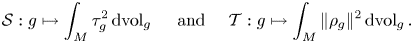
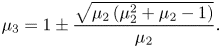
Any $k$ -curvature homogeneous manifold has constant scalar curvature, so equation (1.1) reduces to $\tau ( \rho -\tfrac {1}{3}\tau g )=0$
 . Therefore, for any $k\geq 0$
 , a $k$
 -curvature homogeneous metric is $\mathcal {S}$
 -critical if and only if it is Einstein or its scalar curvature vanishes. Equation (1.3) also simplifies if $\tau$
 is constant and a $k$
 -curvature homogeneous metric is $\mathcal {F}_t$
 -critical if and only if it satisfies

We classify $\mathcal {F}_t$ -critical metrics which are 1-curvature homogeneous but not homogeneous as follows.
Theorem 2.1 Let $(M,\,g)$ be a 1-curvature homogeneous Lorentzian manifold which is not locally homogeneous. Then $g$
 is $\mathcal {F}_t$
 -critical for some $t\in \mathbb {R}$
 if and only if it satisfies one of the following assertions:
(1) $(M,\,g)$
belongs to the class (A) above with $\kappa =0$ and $b\neq 0$. In this case, $g$ is $\mathcal {F}_t$-critical for $t=-\tfrac {1}{2}$.(2) $(M,\,g)$
belongs to the class (B) above. In this case, $g$ is $\mathcal {F}_t$-critical for $t=\frac {\alpha ^{2}+\alpha \beta -\beta ^{2}}{3\beta ^{2}}\geq -\frac {5}{12}$.


Proof. Following [Reference Bueken and Djorić7], since $(M,\,g)$ is a non-homogeneous 1-curvature homogeneous manifold, it either belongs to class (A) or class (B). Assume first that $(M,\,g)$
 belongs to class (A) and let $\{ u_1,\, u_2,\, u_3 \}$
 be a pseudo-orthonormal local frame satisfying $\langle u_1,\, u_1 \rangle =\langle u_2,\, u_3 \rangle =1$
 with Lie brackets given by (2.1). A straightforward calculation shows that
Hence, from equation (2.3), $\Delta \rho (u_3,\,u_3)= -8\kappa (b+2\kappa ^{2})=0$ . So $b=-2\kappa ^{2}$
 or $\kappa =0$
 . In the former case the metric is Einstein, so it is locally homogeneous and must be excluded. If $\kappa =0$
 , then equation (2.3) reduces to $\tfrac {4}{3}b^{2}(1+2t)( u^{1}\otimes u^{1} - u^{2} \otimes u^{3} )=0$
 . Hence $b=0$
 or $t=-\tfrac {1}{2}$
 . If $b=0$
 the manifold is Einstein, so we conclude $t=-\tfrac {1}{2}$
 . This corresponds to assertion (1).
Now we assume that $(M,\,g)$ belongs to class (B). A straightforward calculation shows that

Hence, equation (2.3) reduces to $8\{\alpha ^{2} +\alpha \beta -(1+3t)\beta ^{2}\}\varepsilon \, u^{3} \otimes u^{3} =0$ . Since $\varepsilon,\,\beta \neq 0$
 , we conclude that $t=\frac {\alpha ^{2} +\alpha \beta -\beta ^{2}}{3\beta ^{2}}$
 , which corresponds to assertion (2).
Remark 2.2 Manifolds in theorem 2.1-(1) admit a parallel null line field $\mathfrak {L}=\operatorname {span}\{ u_2\}$ , so they are Brinkmann waves, but not $pp$
 -waves (see § 3.3). Since, moreover, they have non-vanishing constant scalar curvature, they are a particular family of the metrics described in theorem 5.1 of [Reference Brozos-Vázquez, Caeiro-Oliveira and García-Río6].
Remark 2.3 The Ricci operator of manifolds in theorem 2.1-(1) takes the form $\operatorname {Ric}=\operatorname {diag}[0,\,b,\,b]$ . Note that, since these metrics are $\mathcal {F}_t$
 -critical for the value $t=-\frac 12$
 , the functional has zero energy: $\|\rho \|^{2}-\frac 12 \tau ^{2}=0$
 .
.
On the other hand, the Ricci operator of manifolds in theorem 2.1-(2) has a single eigenvalue $\lambda =-2\beta ^{2}$ , which is a double root of the minimal polynomial. This family of manifolds provides $\mathcal {F}_t$
 -critical metrics for all $t \geq -\tfrac {5}{12}$
 . Moreover, the energy of the $\mathcal {F}_t$
 functionals is given by $\|\rho \|^{2}+t \tau ^{2}=(12+36t)\beta ^{4}$
 , so it is positive if $t>-\frac 13$
 , negative if $-\frac {5}{12}\leq t< -\frac 13$
 , and zero if $t=-\frac 13$
 .
.
Remark 2.4 A three-dimensional Lorentzian manifold is locally conformally flat if and only if the Schouten tensor is Codazzi (i.e., $\nabla _XS_{YZ}=\nabla _YS_{XZ}$ ) or, equivalently, if the Cotton tensor vanishes. A straightforward calculation shows that a three-dimensional non-homogeneous $1$
 -curvature homogeneous Lorentzian manifold is locally conformally flat if and only if it corresponds to class (B) with $\beta =-2\alpha$
 , in which case the metric is $\mathcal {F}_t$
 -critical for $t=-\frac {5}{12}$
 . An immediate calculation from the expression of $t$
 in theorem 2.1-(2) shows that a Lorentzian three-dimensional $1$
 -curvature homogeneous (non-homogeneous) manifold is locally conformally flat if and only if it is $\mathcal {F}_t$
 critical for $t=-\frac {5}{12}$
 .
.
Remark 2.5 Any locally conformally flat three-dimensional $0$ -curvature homogeneous Lorentzian manifold that is not $1$
 -curvature homogeneous admits a local pseudo-orthonormal frame $\{ u_1,\,u_2,\,u_3\}$
 with $\langle u_1,\,u_1\rangle =\langle u_2,\,u_3\rangle =1$
 so that (see [Reference Calvaruso10])

where $\Phi,\,\Psi,\,\Xi,\,\Upsilon$ are smooth functions satisfying
where $\varepsilon ^{2}=1$ . A straightforward calculation shows that the Ricci operator has a single eigenvalue $\kappa +\varepsilon$
 , which is a double root of the minimal polynomial. Thus, it is given by

Moreover
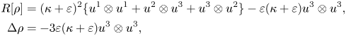
and thus equation (2.3) reduces to $\varepsilon (\kappa +\varepsilon )(12t+5)=0$ . Hence, either $\kappa +\varepsilon =0$
 and $(M,\,g)$
 is critical for all quadratic curvature functionals or, otherwise, it is $\mathcal {F}_t$
 -critical for $t=-\frac {5}{12}$
 . Note that there exist locally conformally flat homogeneous metrics whose Ricci operator has complex eigenvalues which are not critical for any quadratic curvature functional $\mathcal {F}_t$
 . This analysis is carried out in § 5.2.
Remark 2.6 A Lorentzian manifold is said to be semi-symmetric if the curvature tensor satisfies $R(X,\,Y)\cdot R=0$ for all vector fields, where $R(X,\,Y)$
 acts as a derivation on $R$
 . Equivalently, the curvature tensor at each point coincides with that of a symmetric space (but possibly changing from point to point). Hence, if a non-homogeneous $0$
 -curvature homogeneous Lorentzian manifold is semi-symmetric, then the Ricci operator is two-step nilpotent, as in Cahen–Wallach symmetric spaces, or $\operatorname {Ric}=\operatorname {diag}[0,\,\lambda,\,\lambda ]$
 , as in direct products $\mathbb {R}\times N(c)$
 with $N$
 a surface of constant Gauss curvature. As a consequence, the only semi-symmetric $1$
 -curvature homogeneous Lorentzian manifolds which are not locally homogeneous correspond to class (A) with $\kappa =0$
 and $b\neq 0$
 . This shows that a Lorentzian three-dimensional $1$
 -curvature homogeneous (non-homogeneous) manifold is semi-symmetric if and only if it is $\mathcal {F}_t$
 -critical for $t=-\frac {1}{2}$
 . Note that there exist $\mathcal {F}_{-1/2}$
 -critical homogeneous metrics whose Ricci operator has complex eigenvalues and thus they are not semi-symmetric (see § 5.3).
3. Three-dimensional homogeneous Lorentzian spaces
The set of three-dimensional homogeneous Lorentzian manifolds splits into two categories as follows.
Theorem 3.1 [Reference Calvaruso9]
Let $(M,\,g)$ be a three-dimensional connected, simply connected, complete homogeneous Lorentzian manifold. Then, either $(M,\,g)$
 is symmetric, or it is isometric to a three-dimensional Lie group equipped with a left-invariant Lorentzian metric.
The previous result is also true at the local level, therefore a locally homogeneous Lorentzian 3-manifold is either locally symmetric or locally isometric to a Lie group with a left-invariant Lorentzian metric.
3.1 Symmetric manifolds
Indecomposable but not irreducible Lorentzian symmetric spaces are locally isometric to Cahen–Wallach symmetric spaces and, hence, they are a particular family of plane waves [Reference Cahen, Leroy, Parker, Tricerri and Vanhecke8]. Otherwise, three-dimensional symmetric Lorentzian manifolds are of constant sectional curvature or (locally) a product of the form $\mathbb {R}\times N(c)$ , where $N(c)$
 is a Riemannian or a Lorentzian surface of constant Gauss curvature.
Since manifolds of constant sectional curvature are Einstein, they are critical for all quadratic curvature functionals. It has been shown in [Reference Brozos-Vázquez, Caeiro-Oliveira and García-Río6] that Cahen–Wallach symmetric spaces are also critical for all quadratic curvature functionals, whereas products of the form $\mathbb {R}\times N(c)$ are critical for $t=-\frac 12$
 .
.
3.2 Lie groups with left invariant metric
We work at the Lie algebra level. Let $\mathfrak {g}$ be a three-dimensional Lie algebra endowed with a non-degenerate scalar product $\langle \cdot,\, \cdot \rangle : \mathfrak {g} \times \mathfrak {g} \to \mathbb {R}$
 . Let $\times : \mathfrak {g} \times \mathfrak {g} \to \mathfrak {g}$
 be the cross product satisfying $\langle e_i\times e_j,\, e_k \rangle = \det (e_i,\,e_j,\,e_k)$
 for all orthonormal bases $\{e_1,\,e_2,\,e_3\}$
 . The endomorphism $L$
 determined by $L(e_i\times e_j)=[e_i,\,e_j]$
 , $1 \leq i,\, j \leq 3$
 , is referred to as the structure operator of $\mathfrak {g}$
 .
.
3.2.1 Unimodular Lie groups
Three-dimensional unimodular Lie groups are characterized by the self-adjointness of the structure operator $L$ [Reference Milnor19, Reference Rahmani20]. Attending to the Jordan normal form of $L$
 , Rahmani showed in [Reference Rahmani20] that unimodular Lorentzian Lie algebras $(\mathfrak {g},\,\langle,\,\rangle )$
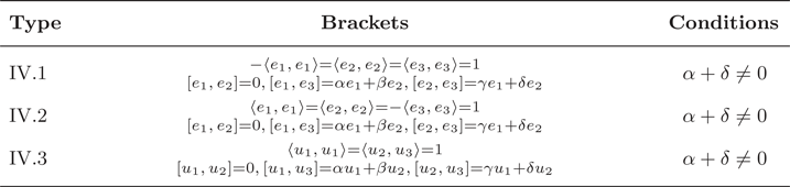
 are equivalent to one of the four types given in table I, where $\{e_1,\,e_2,\,e_3\}$
 and $\{u_1,\,u_2,\,u_3\}$
 are orthonormal and pseudo-orthonormal bases as specified in each case.
TABLE 1. Unimodular Lie algebras

3.2.2 Non-unimodular Lie groups
The Lie algebra of a non-unimodular Lie group is a semi-direct product $\mathfrak {g}=\mathfrak {u}\rtimes \mathbb {R}$ , where $\mathfrak {u}=\{ x\in \mathfrak {g};\, \operatorname {tr}\operatorname {ad}(x)=0\}$
 denotes the unimodular kernel, which is an abelian ideal of $\mathfrak {g}$
 containing the commutator ideal $[\mathfrak {g},\,\mathfrak {g}]$
 (see [Reference Milnor19]). These semi-direct products are determined by the endomorphism $-\operatorname {ad}(e_3)$
 , which does not depend on the choice of $e_3\notin \mathfrak {u}$
 . Thus, for a basis $\{e_1,\,e_2\}$
 of $\mathfrak {u}$
 , the endomorphism $-\operatorname {ad}(e_3)$
 is given by $-\operatorname {ad}(e_3)(e_1)=\alpha e_1 +\beta e_2$
 and $-\operatorname {ad}(e_3)(e_2)=\gamma e_1+\delta e_2$
 . Let $A$
 denote the matrix associated to $-\operatorname {ad}(e_3)$
 .
.
The study of Lorentzian non-unimodular Lie algebras splits into three different situations depending on the restriction of the scalar product $\langle,\,\rangle$ of $\mathfrak {g}$
 to the unimodular kernel $\mathfrak {u}$
 , namely the cases in which $\langle,\,\rangle _{\mid _{\mathfrak {u}\times \mathfrak {u}}}$
 is Lorentzian, Riemannian or degenerate. In each of them there exists an adapted basis so that the Lie algebra is given as in table II.
TABLE 2. Non-unimodular Lie algebras
By rescaling $\{ e_1,\,e_2,\,e_3\}$ one may assume that $\operatorname {tr}\operatorname {ad}(e_3)=2$
 and thus one works with a representative of the homothety class of the initial metric. Moreover, for type IV.3 Lie algebras, taking $\hat {u}_1=u_1$
 , $\hat {u}_2=\frac {\alpha +\delta }{2}u_2$
 and $\hat {u}_3=\frac {2}{\alpha +\delta }u_3$
 , one has that $\operatorname {tr}\operatorname {ad}(u_3)=2$
 and the new basis is still orthonormal, so one remains in the same isometry class.
In the Riemannian situation (see [Reference Milnor19]) one may rotate the orthonormal basis $\{ e_1,\,e_2\}$ so that $\operatorname {ad}(e_3)(e_1)$
 is orthogonal to $\operatorname {ad}(e_3)(e_2)$
 . A straightforward calculation shows that such normalization remains valid in case IV.2 (when the restriction of the inner product to the unimodular kernel is positive definite). Hence one may assume that the structure constants satisfy $\alpha \gamma +\beta \delta =0$
 and $\alpha +\delta =2$
 in this case. This is due to the fact that the self-adjoint part of the endomorphism $\varphi$
 is diagonalizable, a fact that cannot be assumed in the other two cases. The explicit calculations in § 4.5 (remark 4.15) and 4.7 (remark 4.23) show that the analogous normalizations considered in [Reference Cordero and Parker12] for cases IV.1 and IV.3 impose restrictions in the corresponding families of metrics.
3.3 Homogeneous $pp$-waves

In the subsequent analysis of homogeneous critical metrics, we will see that some of the families that show up admit a parallel null line field, as occurs in theorem 2.1-(1). More specifically, some of these examples are $pp$ -waves. Apart from Cahen–Wallach symmetric spaces ($\mathcal {CW}_\varepsilon$
 ), there are other two families of homogeneous $pp$
 -waves. A three-dimensional homogeneous $pp$
 -wave admits local adapted coordinates $(u,\,x,\,y)$
 where the metric is given by $g(\partial _y,\,\partial _y)=-2f(x,\,y)$
 , $g(\partial _y,\,\partial _{u})=g(\partial _x,\,\partial _x)=1$
 . The function $f$
 determines the type of space, which is locally isometric to one of the following models [Reference García-Río, Gilkey and Nikčević13]:
• $\mathcal {N}_b$
is defined by taking $f(x,\,y)=b^{-2}e^{bx}$, with $b\neq 0$,• $\mathcal {P}_c$
is defined by taking $f(x,\,y)=\tfrac {1}{2}x^{2} \alpha (y)$, with $\alpha ' =c\alpha ^{3/2}$ and $\alpha >0$,• $\mathcal {CW}_\varepsilon$
is defined by taking $f(x,\,y)=\varepsilon x^{2}$, with $\varepsilon =\pm 1$.


The geometries $\mathcal {P}_c$ , and $\mathcal {CW}_\varepsilon$
 are plane waves and, jointly with $\mathcal {N}_b$
 , cover all possible homogeneous $pp$
 -wave classes.
Theorem 3.2 Let $(M,\,g)$ be a three-dimensional homogeneous $pp$
 -wave. Then one of the following holds:
(1) If $(M,\,g)$
is a plane wave modelled on $\mathcal {CW}_\varepsilon$ or $\mathcal {P}_c$ then it is critical for all quadratic curvature functionals.(2) If $(M,\,g)$
is a $pp$-wave modelled on $\mathcal {N}_b$ then it is $\mathcal {S}$-critical but not $\mathcal {F}_t$-critical for any $t\in \mathbb {R}$.


Proof. For metrics that belong to the families $\mathcal {P}_c$ and $\mathcal {CW}_\varepsilon$
 , a direct calculation shows that $\Delta \rho$
 , $R[\rho ]$
 , $\Vert \rho \Vert$
 and $\tau$
 vanish identically. Hence, equation (2.3) holds for all $t\in \mathbb {R}$
 and these metrics are critical for all quadratic curvature functionals.
For manifolds modelled on $\mathcal {N}_b$ , the terms $R[\rho ]$
 , $\Vert \rho \Vert$
 and $\tau$
 vanish, but $\Delta \rho (\partial _y,\,\partial _y)=b^{2} e^{bx}\neq 0$
 , since $b\neq 0$
 . Therefore, equation (2.3) is not satisfied for any $t$
 .
.
4. Critical metrics on Lorentzian Lie groups
Based on the classification given in § 3.2, we study Lie groups which admit Lorentzian metrics that are critical for quadratic curvature functionals.
Surprisingly, the Golden number $\varphi =\frac {1+\sqrt {5}}{2}$ plays a distinguished role in describing $\mathcal {F}_t$
 -critical unimodular Lie groups of types Ia, Ib and II. The golden ratio appears not only in the description of left-invariant metrics, as in theorem 4.1 and theorem 4.7, but also on the range of the real parameter $t$
 , as in remark 4.5 (see also Fig. 1).


4.1 Type Ia critical metrics
$G$ is unimodular and there exists an orthonormal basis $\{e_1 (+),\, e_2(+),\, e_3(-)\}$
 such that the structure constants of the Lie algebra $\mathfrak {g}$
 are given by

with $\lambda _1,\, \lambda _2,\, \lambda _3 \in \mathbb {R}$ . The Ricci operator is given by $2\operatorname {Ric}=\operatorname {diag}[(\lambda _2-\lambda _3)^{2}-\lambda _1^{2},\,(\lambda _1-\lambda _3)^{2}-\lambda _2^{2},\,(\lambda _1-\lambda _2)^{2}-\lambda _3^{2}]$
 , hence Einstein metrics in this family are those that satisfy $\lambda _1=\lambda _2=\lambda _3$
 or $\lambda _i=\lambda _j$
 and $\lambda _k=0$
 for $\{i,\,j,\,k\}=\{1,\,2,\,3\}$
 . The scalar curvature for a metric given by (4.1) is $\tau =\frac {\lambda _1^{2}}{2}+\frac {\lambda _2^{2}}{2}+\frac {\lambda _3^{2}}{2}-\lambda _1 \lambda _2 -\lambda _1 \lambda _3 -\lambda _2 \lambda _3$
 . Note that, although this situation is very close to that discussed in [Reference Brozos-Vázquez, Caeiro-Oliveira and García-Río5], since the vector $e_3$
 is timelike, it is not interchangeable with $e_1$
 and $e_2$
 as in the positive definite case.
Theorem 4.1 Let $G$ be a type Ia Lie group with a non-Einstein left-invariant metric. Then $g$
 is $\mathcal {F}_t$
 -critical if and only if it is homothetic to a metric given by (4.1) with structure constants as follows:
(1) $(\lambda _1,\,\lambda _2,\,\lambda _3)=(1,\,\lambda,\,\lambda )$
or $(\lambda _1,\,\lambda _2,\,\lambda _3)=(\lambda,\,\lambda,\,1),$ with $\lambda \neq \frac 14,\,1$. In this case the metric is critical for $t=\frac {3-2\lambda }{-1+4\lambda }$ and $\tau =\frac 12-2\lambda$.(2) $(\lambda _1,\,\lambda _2,\,\lambda _3)=(1,\,\alpha,\,\beta )$
or $(\lambda _1,\,\lambda _2,\,\lambda _3)=(\alpha,\,\beta,\,1),$ with $\alpha \neq \beta$ given by
\[ \begin{array}{l} \alpha=\dfrac{\kappa}2 \pm\dfrac{\sqrt{\kappa \left(\kappa^{2}+\kappa-1\right)}}{2\kappa}, \text{ and } \beta=\dfrac{\kappa}2 \mp\dfrac{\sqrt{\kappa \left(\kappa^{2}+\kappa-1\right)}}{2\kappa}, \end{array} \]where $\kappa \in (-\varphi,\,0)\cup ( \varphi ^{-1},\,\infty ),$
$\kappa \notin \{ 1,\, \varphi ^{3},\, -\varphi ^{-3}\}$. The corresponding metric is critical for the value $t=\frac {\kappa ^{3}+\kappa ^{2}+3 \kappa -1}{(\kappa -1)^{2}}$ and the scalar curvature is given by $\tau =-\frac {(\kappa -1)^{2}}{2 \kappa }$.


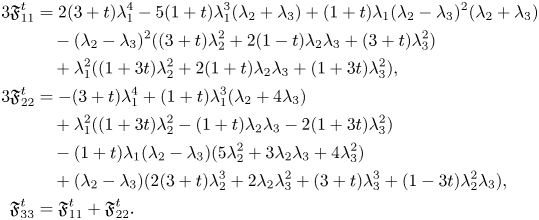
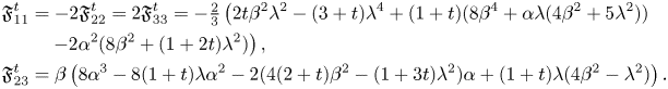
Proof. Motivated by equation (2.3), we define the $(0,\,2)$ -tensor field $\mathfrak {F}^{t} =\Delta \rho +2(R[\rho ]-\tfrac {1}{3}\Vert \rho \Vert ^{2} g)+2t\tau (\rho -\tfrac {1}{3}\tau g)$
 . Thus, $\mathfrak {F}^{t}$
 vanishes if and only if $g$
 is $\mathcal {F}_t$
 -critical. On the pseudo-orthonormal basis $\{e_1,\,e_2,\,e_3\}$
 , $\mathfrak {F}^{t}$
 is given by the following non-vanishing expressions:
Since equation (2.3) is invariant under homotheties, we normalize the constants $(\lambda _1,\,\lambda _2,\,\lambda _3)$ and divide the proof into the following cases, which cover all the non-Einstein possibilities:
(1) Two constants are equal and the third one is nonzero:
(a) $(\lambda _1,\,\lambda _2,\,\lambda _3)=(1,\,0,\,0)$
or $(\lambda _1,\,\lambda _2,\,\lambda _3)=(0,\,0,\,1)$,(b) $(\lambda _1,\,\lambda _2,\,\lambda _3)=(1,\,\lambda,\,\lambda )$
or $(\lambda _1,\,\lambda _2,\,\lambda _3)=(\lambda,\,\lambda,\,1)$, with $\lambda \neq 0,\,1$.
(2) The three constants are different:
(a) $(\lambda _1,\,\lambda _2,\,\lambda _3)=(0,\,\alpha,\,\beta )$
or $(\lambda _1,\,\lambda _2,\,\lambda _3)=(\alpha,\,\beta,\,0)$, with $0\neq \alpha \neq \beta \neq 0$.(b) $(\lambda _1,\,\lambda _2,\,\lambda _3)=(1,\,\alpha,\,\beta )$
or $(\lambda _1,\,\lambda _2,\,\lambda _3)=(\alpha,\,\beta,\,1)$, with $0,\,1\neq \alpha \neq \beta \neq 0,\,1$.


Case (1.a). We consider structure constants $(\lambda _1,\,\lambda _2,\,\lambda _3)=(1,\,0,\,0)$ and $(\lambda _1,\,\lambda _2,\,\lambda _3)=(0,\,0,\,1)$
 . Then, we get, respectively,

Therefore, these metrics are $\mathcal {F}_t$ -critical for $t=-3$
 .
.
Case (1.b). For $(\lambda _1,\,\lambda _2,\,\lambda _3)=(1,\,\lambda,\,\lambda )$ and $(\lambda _1,\,\lambda _2,\,\lambda _3)=(\lambda,\,\lambda,\,1)$
 , with $\lambda \neq 0,\,1$
 , the expressions of $\mathfrak {F}_{ij}^{t}$
 reduce, respectively, to
Hence, since $\lambda \neq 1$ , these terms vanish if and only if $\lambda \neq \frac 14$
 and $t=\frac {3-2\lambda }{-1+4\lambda }$
 .
.
Note that Case (1.a) corresponds to $\lambda =0$ in case (1.b), so this two cases constitute case (1).
Case (2). We work with structure constants $(\lambda _1,\,\lambda _2,\,\lambda _3)$ , all of them different to each other. Then we compute

Note that, if $\tau =0$ , then the metric is not critical for any $t$
 , since $\mathfrak {F}^{t}_{ii}=0$
 implies $\lambda _1=\lambda _2=\lambda _3=0$
 , contrary to our assumption. Hence, we have $\tau \neq 0$
 and the value of $t$
 is given by $t=-\frac {\lambda _1^{2}+\lambda _2^{2}+\lambda _3^{2}}{\tau }$
 . Taking the value of $t$
 into account, the expressions of $\mathfrak {F}_{ii}^{t}$
 reduce to

Since the values of $\lambda _1$ , $\lambda _2$
 and $\lambda _3$
 are all distinct, the first factors in these expressions cannot vanish simultaneously. Hence, we have

Note that this equation and the value of $t$ are symmetric in the $\lambda$
 's, so we work modulo permutation.
Case (2.a). Assume that $\lambda _1=0$ . Then $(\lambda _2-\lambda _3)^{2} (\lambda _2+\lambda _3)=0$
 , so $\lambda _2=- \lambda _3$
 . We have two homothety classes: $(0,\,1,\,-1)$
 and $(1,\,-1,\,0)$
 . In both cases the corresponding left invariant metrics are critical for $t=-1$
 and the Ricci operator satisfies $\operatorname {Ric}=\operatorname {diag}[2 ,\,0,\,0]$
 and $\operatorname {Ric}=\operatorname {diag}[0,\,0,\,2]$
 , respectively.
Case (2.b). Now we consider the case $\lambda _1\neq 0$ . The obtained expressions coincide with those studied in the Riemannian analogue in [Reference Brozos-Vázquez, Caeiro-Oliveira and García-Río5]. Rescaling the metric so that $\lambda _1=1$
 and setting $\lambda _2=\frac {-1+\mu _2+\mu _3}2$
 and $\lambda _3=\frac {1+\mu _2-\mu _3}2$
 , expression (4.2) reduces to
Then, solving in $\mu _3$ , one has
Note that $\mu _3$ is well-defined if $\mu _2\in (-\varphi,\,0)$
 or $\mu _2>\varphi ^{-1}$
 . Hence, set $\mu _2=\kappa$
 to see that, for structure constants $\lambda _i\neq \lambda _j$
 if $i\neq j$
 , the corresponding metric is $\mathcal {F}_t$
 -critical if and only if it is homothetic to a metric given by $\lambda _1=1$
 ,
,

The structure constants $(1,\,\lambda _2,\,\lambda _3)$ are distinct except if $\kappa =1$
 , $\kappa ={ \varphi ^{3}}$
 or $\kappa ={-\varphi ^{-3}}$
 . Note that for $\kappa =- 1$
 we get that $\lambda _3=0$
 . Thus, this case includes case (2.a).
If we choose to normalize $\lambda _3=1$ , then we obtain another homothety family with values for $\lambda _1$
 and $\lambda _2$
 given by the expressions of $\lambda _2$
 and $\lambda _3$
 in (4.3). Also, for appropriate $\kappa$
 we recover the case $\lambda _1=0$
 . This concludes case (2).
Remark 4.2 The family given in theorem 4.1-(1) provides critical metrics for all $t \in \mathbb {R} \setminus \{ -\tfrac {1}{2} \}$ . Whereas the family given in theorem 4.1-(2) provides $\mathcal {F}_t$
 -critical metrics for $t \in (-1-\varphi ^{-5},\,-1)$
 if $\kappa \in (-\varphi,\,0)\backslash \{-\varphi ^{-3}\}$
 and for $t \in (-1+\varphi ^{5},\, +\infty )$
 if $\kappa \in ( \varphi ^{-1},\,\infty )\setminus \{1,\, \varphi ^{3}\}$
 . These values of $t$
 are illustrated in figure 1.
Remark 4.3 Lie algebras obtained in theorem 4.1-(1) are $\mathfrak {h}_3$ if $\lambda =0$
 (case (1.a) in the proof), $\mathfrak {sl}(2,\,\mathbb {R})$
 if $(\lambda _1,\,\lambda _2,\,\lambda _3)=(1,\,\lambda,\,\lambda )$
 , $\lambda \neq 0$
 , or $(\lambda _1,\,\lambda _2,\,\lambda _3)=(\lambda,\,\lambda,\,1)$
 with $\lambda > 0$
 , and $\mathfrak {su}(2)$
 if $(\lambda _1,\,\lambda _2,\,\lambda _3)=(\lambda,\,\lambda,\,1)$
 with $\lambda <0$
 .
.
Lie algebras obtained in theorem 4.1-(2) with one zero constant (case (2.a) in the proof) are $\mathfrak {e}(1,\,1)$ if $(\lambda _1,\,\lambda _2,\,\lambda _3)=(\lambda,\,-\lambda,\,0)$
 or $\mathfrak {e}(2)$
 if $(\lambda _1,\,\lambda _2,\,\lambda _3)=(0,\,\lambda,\,-\lambda )$
 . This is in sharp contrast with the Riemannian setting, where the Euclidean group does not admit any $\mathcal {F}_t$
 -critical metric which is not Einstein.
In the theorem 4.1-(2) with no zero constant (case (2.b) in the proof) we have that:
• The Lie algebra is $\mathfrak {sl}(2,\,\mathbb {R})$
if $(\lambda _1,\,\lambda _2,\,\lambda _3)=(1,\,\alpha,\,\beta )$ with $\alpha,\,\beta <0$, which occurs if $\kappa \in (-\varphi,\,-1)$, or if $\alpha <0,\, \beta >0$, which can occur if $\kappa \in (-1,\,0)$.• The Lie algebra is $\mathfrak {su}(2)$
if $(\lambda _1,\,\lambda _2,\,\lambda _3)=(1,\,\alpha,\,\beta )$ with $\alpha >0,\,\beta <0$, which can occur if $\kappa \in (-1,\,0)$.• The Lie algebra is $\mathfrak {sl}(2,\,\mathbb {R})$
if $(\lambda _1,\,\lambda _2,\,\lambda _3)=(\alpha,\,\beta,\,1)$ with $\alpha,\,\beta >0$, which occurs if $\kappa >\varphi ^{-1}$, or $\alpha$ and $\beta$ have different sign, which occurs if $\kappa \in (-1,\,0)$.• The Lie algebra is $\mathfrak {su}(2)$
if $(\lambda _1,\,\lambda _2,\,\lambda _3)=(\alpha,\,\beta,\,1)$ with $\alpha,\,\beta <0$, which occurs if $\kappa \in (-\varphi,\,-1)$.


4.2 Type Ib critical metrics
$G$ is unimodular and there exists an orthonormal basis $\{e_1(+),\, e_2(+),\, e_3(-)\}$
 such that the Lie brackets of the Lie algebra $\mathfrak {g}$
 are given by

with $\alpha,\, \beta,\, \lambda \in \mathbb {R}$ , $\beta \neq 0$
 . Further observe that a replacement $e_1\mapsto -e_1$
 provides an isometry interchanging $(\alpha,\,\beta,\,\lambda )$
 with $(-\alpha,\,-\beta,\,-\lambda )$
 , whereas $e_2\mapsto -e_2$
 or $e_3\mapsto -e_3$
 interchanges $(\alpha,\,\lambda )$
 with $(-\alpha,\,-\lambda )$
 , hence one may assume $\beta >0$
 .
.
Metrics defined by (4.4) are not Einstein and they have scalar curvature $\tau =\frac {1}{2}(\lambda (\lambda -4\alpha )-4\beta ^{2})$ . Hence they are $\mathcal {S}$
 -critical if and only if $\lambda =2(\alpha \pm \sqrt {\alpha ^{2}+\beta ^{2}})$
 .
.
Theorem 4.4 Let $G$ be a type Ib Lie group with a left-invariant metric $g$
 . Then $g$
 is $\mathcal {F}_t$
 -critical if and only if it is isometric to a metric given by (4.4) with structure constants satisfying one of the following conditions:
(1) $8 \alpha \beta ^{2} =\lambda (\lambda -2\varphi \alpha ) (\lambda +2\varphi ^{-1}\alpha ),$
$\alpha \neq 0$. In this case, $G$ is isomorphic to $SL(2,\,\mathbb {R})$ and $g$ is $\mathcal {F}_t$-critical for $t=\frac {8 \alpha ^{3} +4 \alpha ^{2} \lambda +6 \alpha \lambda ^{2} -\lambda ^{3}}{\lambda (\lambda -2\alpha )^{2}}$.(2) $\alpha =\lambda =0$
. In this case, $G$ is isomorphic to $E(1,\,1)$ and the metric $g$ is $\mathcal {F}_t$-critical for $t=-1$.


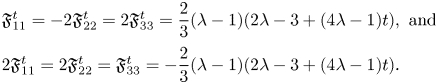
Proof. A straightforward computation shows that the possibly non-vanishing terms of $\mathfrak {F}^{t}$ with respect to the basis $\{e_1,\,e_2,\,e_3\}$
 are the following:
We first consider the case in which the scalar curvature vanishes. If $\tau =4\beta ^{2} +(4\alpha -\lambda )\lambda =0$ , then $\mathfrak {F}_{23}^{t}=-\beta (-8 \alpha ^{3} + 16 \alpha \beta ^{2} + 8 \alpha ^{2} \lambda - 4 \beta ^{2} \lambda - 2 \alpha \lambda ^{2} + \lambda ^{3})$
 and there are two possibilities: either $\alpha =0$
 and $\lambda = \pm 2\beta$
 , or $\alpha =-\tfrac {3}{2}\lambda$
 and $\beta =\pm \tfrac {\sqrt {7}}{2}\lambda$
 . The term $\mathfrak {F}_{11}^{t}$
 is given by $\mathfrak {F}_{11}^{t}= 80\beta ^{4}/3$
 and $\mathfrak {F}_{11}^{t}= 2048 \beta ^{4}/147$
 , respectively. Hence $\mathfrak {F}_{11}^{t}$
 does not vanish and these metrics are critical for $\mathcal {S}$
 , but they are not critical for any $\mathcal {F}_t$
 functional.
Now, if $\tau \neq 0$ , a direct analysis of the expression of $\mathfrak {F}_{23}^{t}$
 shows that it vanishes if and only if one of the following assertions holds:
(i) $t=\frac {8\alpha ^{3} -8\alpha ^{2}\lambda +4\beta ^{2} \lambda -\lambda ^{3} +2\alpha (\lambda ^{2} -8\beta ^{2})}{(2\alpha -\lambda )\tau }$
,(ii) $\alpha =\lambda =0$
.


In case (i), one has $(6\alpha -3\lambda )\mathfrak {F}_{11}^{t}=4((\alpha -\lambda )^{2}+\beta ^{2}) (4 \alpha ^{2} \lambda +2 \alpha (4 \beta ^{2}+\lambda ^{2})-\lambda ^{3})$ . Since $\beta \neq 0$
 , the only possibility for $\mathfrak {F}_{11}^{t}$
 to vanish is that $\beta ^{2}=\frac {\lambda }{8 \alpha }(\lambda ^{2} -2\alpha \lambda -4\alpha ^{2})$
 , which corresponds to case (1) in the theorem.
In case (ii), $\mathfrak {F}_{11}^{t}$ reduces to $\mathfrak {F}_{11}^{t}= -16(1+t)\beta ^{4}/3$
 . Hence $t=-1$
 . This is case(2).
Remark 4.5 The family shown in theorem 4.4-(1) gives critical metrics for all $t \in (-\infty,\,-1-\varphi ^{-5}) \cup (-1,\,-1+\varphi ^{5})$ . These values of $t$
 are illustrated in figure 1.
Remark 4.6 The Ricci operators of critical metrics in theorem 4.4-(1) have eigenvalues $\{ {\lambda (\alpha -\frac {\lambda ^{2}}{4\alpha })},\, -\frac {1}{4\alpha }(2\alpha -\lambda )(2\alpha \lambda \pm \sqrt {2\alpha \lambda (4\alpha ^{2} +2\alpha \lambda -\lambda ^{2})})\}$ . Note that, since $\alpha \lambda (4\alpha ^{2} +2\alpha \lambda -\lambda ^{2})=-8 \alpha ^{2}\beta ^{2}< 0$
 , there are two complex conjugate eigenvalues. In contrast, the Ricci operator of metrics in theorem 4.4-(2) is diagonalizable with eigenvalues $\{0,\,0,\,-2\beta ^{2}\}$
 .
.
4.3 Type II critical metrics
$G$ is unimodular and there exists a pseudo-orthonormal basis $\{u_1,\, u_2,\, u_3\}$
 , with $\langle u_1,\,u_2 \rangle =\langle u_3,\,u_3 \rangle =1$
 , such that the Lie brackets of the Lie algebra $\mathfrak {g}$
 are given by

with $\lambda _1,\, \lambda _2 \in \mathbb {R}$ , $\varepsilon =\pm 1$
 . These metrics are Einstein if and only if they are Ricci flat, which occurs if and only if $\lambda _1=\lambda _2=0$
 . Furthermore, the scalar curvature is given by $\tau =\frac 12 \lambda _2 ( \lambda _2-4 \lambda _1 )$
 , so metrics given by (4.5) are $\mathcal {S}$
 -critical if and only if $\lambda _2=0$
 or $\lambda _2=4\lambda _1$
 .
.
Theorem 4.7 Let $G$ be a type II Lie group with a non-Einstein left-invariant metric $g$
 . If $g$
 is $\mathcal {F}_t$
 -critical, then $G$
 is isomorphic to $SL(2,\,\mathbb {R})$
 and $g$
 is isometric to a metric given by (4.5) with structure constants satisfying one of the following:
(1) $\lambda _1=\lambda _2 \neq 0$
. In this case, $g$ is $\mathcal {F}_t$-critical for $t=\frac {1}{3}$.(2) $\lambda _1=-\frac {1}{2}\varphi \lambda _2 \neq 0$
. In this case, $g$ is $\mathcal {F}_t$-critical for $t=-1-\varphi ^{-5}$.(3) $\lambda _1=\frac {1}{2}\varphi ^{-1}\lambda _2 \neq 0$
. In this case, $g$ is $\mathcal {F}_t$-critical for $t=-1+\varphi ^{5}$.


Proof. We compute $\mathfrak {F}^{t} =\Delta \rho +2(R[\rho ]-\tfrac {1}{3}\Vert \rho \Vert ^{2} g)+2t\tau (\rho -\tfrac {1}{3}\tau g)$ in the basis $\{u_1,\,u_2,\,u_3\}$
 , which is determined by
$\mathfrak {F}_{12}^{t}$ vanishes if and only if $\lambda _2=0$
 , $\lambda _1=\lambda _2$
 or $\lambda _2\neq 4\lambda _1$
 and $t=\frac {-2\lambda _1 +3\lambda _2}{4\lambda _1 -\lambda _2}$
 .
.
If $\lambda _2=0$ , then $\mathfrak {F}_{11}^{t}=8\varepsilon \lambda _1^{3}$
 . Thus $\lambda _1=\lambda _2=0$
 and the manifold is Ricci-flat.
If $\lambda _1=\lambda _2$ , it follows that $\mathfrak {F}_{11}^{t} =(1-3t)\varepsilon \lambda _2^{3}$
 . Hence, since $\lambda _1=\lambda _2=0$
 corresponds to an Einstein metric, we conclude that $t= \tfrac {1}{3}$
 . This is case (1).
Now, assume $\lambda _2\neq 0$ , $\lambda _1\neq \lambda _2$
 and $\lambda _2\neq 4\lambda _1$
 . If $t=\frac {-2\lambda _1 +3\lambda _2}{4\lambda _1 -\lambda _2}$
 , then $\mathfrak {F}_{11}^{t}=2\varepsilon (\lambda _1-\lambda _2)(4\lambda _1^{2} +2\lambda _1\lambda _2-\lambda _2^{2})$
 . Hence $4\lambda _1^{2} +2\lambda _1\lambda _2-\lambda _2^{2}=0$
 , so $\lambda _1=-\frac {\varphi }{2}\lambda _2$
 , which corresponds to case (2), or $\lambda _1=- \varphi ^{-1}\lambda _2$
 , which corresponds to case (3).
Remark 4.8 Metrics given by (4.5) have Ricci curvatures $a=-\frac {1}{2}\lambda _2^{2}$ and $b$
 given by $b=-\frac {1}{2}\lambda _2^{2}$
 in theorem 4.7-(1), $b=\frac {1}{2}\varphi ^{2}\lambda _2^{2}$
 in theorem 4.7-(2), and $b=\frac {1}{2}\varphi ^{-2}\lambda _2^{2}$
 in theorem 4.7-(3). Moreover, the eigenvalue $b$
 is always a double root of the corresponding minimal polynomial.
Remark 4.9 Left-invariant metrics given by (4.5) with $\lambda _2=0$ have a null parallel line field $\mathfrak {L}=\operatorname {span}\{ u_2\}$
 and two-step nilpotent Ricci operator. Hence they are $pp$
 -waves and correspond to one of the cases in theorem 3.2. Since no non-Einstein metric with $\lambda _2=0$
 may be $\mathcal {F}_t$
 -critical by theorem 4.7, they correspond to metrics in theorem 3.2-(2), so they are locally isometric to $pp$
 -waves in the family $\mathcal {N}_b$
 .
.
4.4 Type III critical metrics
$G$ is unimodular and there exists a pseudo-orthonormal basis $\{u_1,\, u_2,\, u_3\}$
 , with $\langle u_1,\,u_2 \rangle =\langle u_3,\,u_3 \rangle =1$
 , such that the Lie brackets of the Lie algebra $\mathfrak {g}$
 are given by

with $\lambda \in \mathbb {R}$ . There are no Einstein metrics in this family. Moreover, the scalar curvature is given by $\tau =-\frac 32 \lambda ^{2}$
 , so metrics defined by (4.6) are $\mathcal {S}$
 -critical if and only if $\lambda =0$
 .
.
Theorem 4.10 Let $G$ be a type III Lie group with a left-invariant metric $g$
 . Then $g$
 is $\mathcal {F}_t$
 -critical if and only if $G$
 is isomorphic to $E(1,\,1)$
 and $g$
 is isometric to a metric given by (4.6) with $\lambda =0$
 . In this case, the metric is critical for all $t\in \mathbb {R}$
 .
.
Proof. With respect to the pseudo-orthonormal basis $\{u_1,\,u_2,\,u_3\}$ , $\mathfrak {F}^{t}$
 is determined by the following expressions:

Thus, $\mathfrak {F}^{t}$ vanishes identically if and only if $\lambda =0$
 .
.
Remark 4.11 Left-invariant metrics in theorem 4.10 have a null parallel line field $\mathfrak {L}=\operatorname {span}\{ u_1\}$ . Moreover, the Ricci operator is two-step nilpotent, and thus they are $pp$
 -waves. Since no metric in theorem 4.10 is locally symmetric, they correspond to metrics given in theorem 3.2-(1), so they are locally isometric to plane waves in the family $\mathcal {P}_c$
 .
.
4.5 Type IV.1: critical metrics with Lorentzian unimodular kernel
$G$ is non-unimodular and the induced metric on the unimodular kernel $\mathfrak {u}$
 is Lorentzian. Then there exists an orthonormal basis $\{e_1(-),\, e_2(+),\, e_3(+)\}$
 such that the Lie algebra $\mathfrak {g}$
 is given by

with $\alpha,\, \beta,\, \gamma,\, \delta \in \mathbb {R}$ . We work with a representative of the homothety class so that $\alpha +\delta =2$
 . These metrics are Einstein for the following values of $\alpha$
 , $\beta$
 and $\gamma$
 :
:
(i) $\alpha =1$
and $\gamma =\beta$,(ii) $\beta =\pm \alpha$
and $\gamma =\pm (2-\alpha )$.


Note that the case $A=\operatorname {ad}(e_3)=\operatorname {\rm Id}$ is included in $(i)$
 . Also, note that the structure given by $(\beta,\,\gamma )=(\alpha,\,2-\alpha )$
 is isometric to $(\beta,\,\gamma )=(-\alpha,\,\alpha -2)$
 since the replacement $e_1\mapsto -e_1$
 provides an isometric isomorphism interchanging $(\beta,\,\gamma )$
 and $(-\beta,\,-\gamma )$
 . The scalar curvature has the expression $\tau =\frac {1}{2} (-4 (\alpha -2) \alpha +(\beta -\gamma )^{2}-16)$
 . Thus metrics given by (4.7) are $\mathcal {S}$
 -critical if and only if $\alpha =1\pm \frac {1}{2}\sqrt {(\beta -\gamma )^{2}-12}$
 or the manifold is Einstein.
Theorem 4.12 Let $G$ be a type IV.1 Lie group. A non-Einstein left-invariant metric $g$
 on $G$
 is $\mathcal {F}_t$
 -critical if and only if it is homothetic to a metric given by (4.7) with structure constants as follows:
(1) $\alpha =1 + \tfrac {1}{2}(\beta -\gamma )$
. In this case, $g$ is $\mathcal {F}_t$-critical for $t=-\tfrac {1}{3}(\det A+\sqrt {1-\det A})$ and $\det A \leq 1$.(2) $\det A =0$
. In this case, $g$ is $\mathcal {F}_t$-critical for $t=-\frac {3(\beta +\gamma )^{2}-8}{(\beta +\gamma )^{2} -16}$.(3) The derivation $\operatorname {ad}(e_3)$
is self-adjoint, i.e. $\beta =-\gamma$. In this case, $g$ is $\mathcal {F}_t$-critical for $t=-\frac {2-\det A}{4- \det A}$. Moreover, $\det A$ takes all possible real values and $A$ realizes all possible Jordan normal forms.


Proof. The symmetric (0,2)-tensor field $\mathfrak {F}^{t} =\Delta \rho +2(R[\rho ]-\tfrac {1}{3}\Vert \rho \Vert ^{2} g)+2t\tau (\rho -\tfrac {1}{3}\tau g)$ is given, with respect to the basis $\{e_1,\,e_2,\,e_3\}$
 , by the following components:
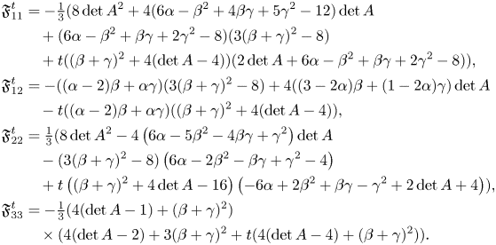
A straightforward calculation shows that $\mathfrak {F}_{33}^{t}$ vanishes if and only if $\det A = 1-\frac {(\beta +\gamma )^{2}}{4}$
 or $t=-\frac {4(\det A-2)+3(\beta +\gamma )^{2}}{4(\det A-4) +(\beta +\gamma )^{2}}$
 .
.
Firstly, we assume $\det A = 1-\frac {(\beta +\gamma )^{2}}{4}$ , then $\alpha =1 \pm \tfrac {1}{2}(\beta -\gamma )$
 . Since $(\beta,\,\gamma )\to (-\beta,\,-\gamma )$
 provides an isometry, we assume without loss of generality that $\alpha =1 + \tfrac {1}{2}(\beta -\gamma )$
 . The components of $\mathfrak {F}^{t}$
 simplify to

If $\beta =\gamma$ , then $\alpha =1$
 and the metric is Einstein. If $\gamma =2-\beta$
 , then $\alpha =\beta$
 and the metric is also Einstein. Hence $t=-\tfrac {1}{6}(2\det A +\beta +\gamma )$
 , which corresponds to case (1).
Secondly, we assume $t=-\frac {4(\det A-2)+3(\beta +\gamma )^{2}}{4(\det A-4) +(\beta +\gamma )^{2}}$ . The components of $\mathfrak {F}^{t}$
 reduce to

Thus, the tensor $\mathfrak {F}^{t}$ vanishes if $\det A=0$
 , which corresponds to case (2), if $\beta =-\gamma$
 , which corresponds to case (3), or if $\alpha =1$
 and $\beta =\gamma$
 , which is an Einstein metric.
Remark 4.13 Metrics in theorem 4.12 provide examples of $\mathcal {F}_t$ -critical metrics for values of $t$
 in $\mathbb {R} \setminus \{-1\}$
 . The attained values in each of the cases are illustrated in figure 2 and are described as follows:
• Case (1) provides $\mathcal {F}_t$
-critical metrics for $t \in (-\tfrac {5}{12},\,\infty )$ with energy $\|\rho \|^{2}+t\tau ^{2}=3 (\beta +\gamma )(\beta +\gamma -2)$.• Case (2) provides $\mathcal {F}_t$
-critical metrics for $t \in (-\infty,\, -3) \cup (-\tfrac {1}{2},\, +\infty )$ with energy $\|\rho \|^{2}+t\tau ^{2}=6 (\beta +\gamma )^{2}$.• Case (3) provides $\mathcal {F}_t$
-critical metrics for all $t \in \mathbb {R} \setminus \{-1\}$ with zero energy.


For any non-Einstein critical metric, observe that the energy of the corresponding functional $\mathcal {F}_t$ is zero if and only if $\beta =-\gamma$
 .
.


Remark 4.14 The Ricci operator of critical metrics in theorem 4.12 is determined as follows:
• Critical metrics corresponding to case (1) have a single Ricci curvature equal to $-2$
, which is a double root of the minimal polynomial.• Critical metrics in case (2) have diagonalizable Ricci operator with two-distinct Ricci curvatures $\operatorname {Ric}=-\operatorname {diag}[\tfrac {1}{2}(\beta +\gamma )^{2},\, 4-\tfrac {1}{2}(\beta +\gamma )^{2},\, 4-\tfrac {1}{2}(\beta +\gamma )^{2}]$
.• The Ricci operator of critical metrics corresponding to case (3) has eigenvalues $\{-2(2-\det A),\, -2(1\pm \sqrt {1-\det A}\}$
, which may be real or complex depending on the value of $\det A$. Furthermore if $\operatorname {det}A=1$, there is a single eigenvalue which is a double root of the minimal polynomial.


Remark 4.15 Theorem 4.12 shows that the normalization $\operatorname {ad}(e_3)(e_1)\perp \operatorname {ad}(e_3)(e_2)$ considered in [Reference Cordero and Parker12] is not always possible. Indeed, left-invariant metrics in theorem 4.12-(3), where $A$
 is self-adjoint, satisfy the above normalization only if $A$
 diagonalizes. Thus, the cases with complex eigenvalues and a double root of the minimal polynomial are missed if one assumes the possibility of normalizing as above. Indeed, if one considers metrics given by (4.7) with $\alpha \gamma -\beta \delta =0$
 , no $\mathcal {F}_t$
 -critical metric is found with $t\in (-3,\,-\frac 12)$
 .
.
4.6 Type IV.2: critical metrics with Riemannian unimodular kernel
$G$ is non-unimodular and the induced metric on the unimodular kernel $\mathfrak {u}$
 is Riemannian. Then there exists an orthonormal basis $\{e_1(+),\, e_2(+),\, e_3(-)\}$
 such that the Lie algebra $\mathfrak {g}$
 is given by

with $\alpha,\, \beta,\, \gamma,\, \delta \in \mathbb {R}$ satisfying $\alpha +\delta =2$
 . A direct calculation shows that these metrics are Einstein if and only if $\alpha =1$
 and $\gamma =-\beta$
 (which includes the case $\operatorname {ad}(e_3)=\operatorname {\rm Id}$
 ). Moreover, the scalar curvature is given by $\tau =\frac {1}{2} (4 (\alpha -2) \alpha +(\beta +\gamma )^{2}+16)$
 and satisfies $\tau >0$
 . Hence the only $\mathcal {S}$
 -critical metrics within this family are the Einstein ones.
Theorem 4.16 Let $G$ be a type IV.2 Lie group. A non-Einstein left-invariant metric $g$
 on $G$
 is $\mathcal {F}_t$
 -critical if and only if it is homothetic to a metric given by (4.8) with structure constants as follows:
(1) $\det A=0$
. In this case, $g$ is $\mathcal {F}_t$-critical for $t=-\frac {8+3(\beta -\gamma )^{2}}{16+(\beta -\gamma )^{2}}$.(2) The derivation $\operatorname {ad}(e_3)$
is self-adjoint, i.e. $\beta =\gamma$. In this case, $g$ is $\mathcal {F}_t$-critical for $t=-\frac {2-\det A}{4-\det A}$ and $\det A < 1$.


Proof. On the pseudo-orthonormal basis $\{e_1,\,e_2,\,e_3\}$ , the a priori non-vanishing components of $\mathfrak {F}^{t}$
 are given by the following expressions:
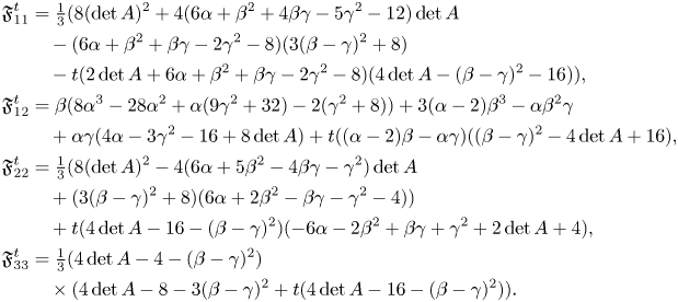
A straightforward calculation shows that $\mathfrak {F}_{33}^{t}$ vanishes if and only if $\det A=1 +\tfrac {1}{4}(\beta -\gamma )^{2}$
 or $t=-\frac {4\det A -8 -3(\beta -\gamma )^{2}}{4\det A -16 -(\beta -\gamma )^{2}}$
 . Since $\det A=-\alpha ^{2}+2 \alpha -\beta \gamma$
 , the equation $\det A=1 +\tfrac {1}{4}(\beta -\gamma )^{2}$
 has real solutions only if $\beta =-\gamma$
 , in which case $\alpha =1$
 . Hence, this condition leads to an Einstein metric.
Hence, we assume $t=-\frac {4\det A -8 -3(\beta -\gamma )^{2}}{4\det A -16 -(\beta -\gamma )^{2}}$ . Simplifying the components of $\mathfrak {F}^{t}$
 , we get:
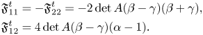
Thus the tensor $\mathfrak {F}^{t}$ vanishes if $\det A=0$
 , which corresponds to case (1), if $\beta =\gamma$
 , which corresponds to case (2), or if $\alpha =1$
 and $\beta =-\gamma$
 , which corresponds to an Einstein metric.
Remark 4.17 Notice that the family of metrics in theorem 4.16-(2) gives critical metrics for all $t \in (-1,\,-\tfrac {1}{3})$ with zero energy, whereas the family of metrics in theorem 4.16-(1) gives critical metrics for all $t \in (-3,\,-\tfrac {1}{2}]$
 with energy given by $\|\rho \|^{2}+t\tau ^{2}=-6(\beta -\gamma )^{2}$
 . The value $t=-\frac 12$
 for metrics with $\beta =\gamma$
 corresponds to critical metrics which are Einstein ($\alpha =1$
 , $\beta =\gamma =0$
 ). These values of $t$
 are illustrated in Fig. 2.
Remark 4.18 The Ricci operator of critical metrics obtained in theorem 4.16 is diagonalizable with eigenvalues
(1) $\left \{4+\tfrac {1}{2}(\beta -\gamma )^{2},\, 4+\tfrac {1}{2}(\beta -\gamma )^{2},\, -\tfrac {1}{2}(\beta -\gamma )^{2}\right \}$
,(2) $\left \{2(2-\det A),\, 2(1-\sqrt { 1-\det A}),\,2(1+\sqrt {1-\det A})\right \}$
.


Remark 4.19 The Lie algebra given by (4.8) corresponds to a semi-direct product $\mathbb {R}\ltimes \mathfrak {r}^{2}$ where the metric restricted to $\mathfrak {r}^{2}$
 has positive definite signature. Therefore, the results are analogous to those obtained for three-dimensional Riemannian non-unimodular Lie groups (cf. [Reference Brozos-Vázquez, Caeiro-Oliveira and García-Río5]).
4.7 Type IV.3: critical metrics with degenerate unimodular kernel
$G$ is non-unimodular and the restriction of the metric to the unimodular kernel $\mathfrak {u}$
 is degenerate. Then there exists a pseudo-orthonormal basis $\{u_1,\, u_2,\, u_3\}$
 of the Lie algebra, with $\langle u_1,\,u_1 \rangle =\langle u_2,\,u_3 \rangle =1$
 , such that

with $\alpha,\, \beta,\, \gamma,\, \delta \in \mathbb {R}$ , and $\alpha +\delta =2$
 . These metrics are Einstein only if they are flat, which occurs if $\gamma =0$
 and $\alpha =0,\,1$
 . Moreover, the scalar curvature is $\tau =\frac {\gamma ^{2}}2$
 , so metrics given by (4.9) are $\mathcal {S}$
 -critical if and only if $\gamma =0$
 .
.
Theorem 4.20 Let $G$ be a type IV.3 Lie group. A non-Einstein left-invariant metric $g$
 on $G$
 is $\mathcal {F}_t$
 -critical if and only if it is homothetic to a metric given by (4.9) with structure constants as follows:
(1) $\det A=0$
. In this case, $g$ is $\mathcal {F}_t$-critical for $t=-3$.(2) The derivation $\operatorname {ad}(e_3)$
is self-adjoint, i.e., $\gamma =0$. In this case, $g$ is $\mathcal {F}_t$-critical for all $t\in \mathbb {R}$.


Proof. The a priori non-vanishing components of the tensor field $\mathfrak {F}^{t}$ are given, with respect to the $\{u_1,\,u_2,\,u_3\}$
 basis, by
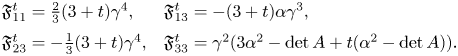
$\mathfrak {F}_{11}^{t}$ vanishes if and only if $\gamma =0$
 or $t=-3$
 . If $\gamma =0$
 , the tensor field vanishes identically with independence of the value of $t$
 . This corresponds to case (2).
Now, we assume $\gamma \neq 0$ and $t=-3$
 . The only non-vanishing component is $\mathfrak {F}_{33}^{t}= 2\gamma ^{2} \det A$
 , that vanishes if and only if $\det A=0$
 . This corresponds to case (1).
Remark 4.21 The Ricci operator of metrics corresponding to theorem 4.20-(1) is diagonalizable with eigenvalues $\{ -\frac{\gamma ^{2}}{2},\, \frac{\gamma ^{2}}{2},\,\frac{\gamma ^{2}}{2}\}$ from where it also follows that the energy vanishes in this case ($\|\rho \|^{2}-3\tau ^{2}=0$
 ).
).
Remark 4.22 Left-invariant metrics in theorem 4.20-(2) have a parallel degenerate line field $\mathfrak {L}=\operatorname {span}\{u_2\}$ . Moreover, the Ricci operator is two-step nilpotent, so they are $pp$
 -waves. In the non-flat case, if $\alpha =2$
 , then they are locally symmetric and, hence, a Cahen–Wallach symmetric space $\mathcal {CW}_\varepsilon$
 . Otherwise, they are plane waves $\mathcal {P}_c$
 (see theorem 3.2). Furthermore, since the Ricci operator is two-step nilpotent, all functionals $\mathcal {F}_t$
 have zero energy in this case.
Remark 4.23 The Ricci operator of any metric (4.9) satisfies
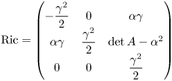
with eigenvalues $\left \{-\frac {\gamma ^{2}}2,\,\frac {\gamma ^{2}}2,\,\frac {\gamma ^{2}}2\right \}$ . Considering the subfamily given by $\alpha ^{2}=\operatorname {det}A$
 one has that the minimal polynomial of the Ricci operator is $(\lambda +\frac {\gamma ^{2}}2)(\lambda -\frac {\gamma ^{2}}2)$
 if $\alpha \gamma =0$
 , but it is $(\lambda +\frac {\gamma ^{2}}2)(\lambda -\frac {\gamma ^{2}}2)^{2}$
 if $\alpha \gamma \neq 0$
 . Hence there are metrics within this subfamily which are not isometric to any metric obtained with the normalization $\alpha \gamma =0$
 proposed in [Reference Cordero and Parker12]. Therefore, the normalization $\operatorname {ad}(e_3)(e_1)\perp \operatorname {ad}(e_3)(e_2)$
 (equivalently $\alpha \gamma =0$
 ) in (4.9) cannot be applied if one intends to consider representatives of all metrics.
5. Special cases
5.1 Critical metrics for the L$^{2}$-norm of the curvature tensor

In dimension three a metric is critical for the curvature functional $g\mapsto \int _M\| R_g\|^{2}\operatorname {dvol}_g$ if and only if it is $\mathcal {F}_t$
 -critical for $t=-\frac {1}{4}$
 . The first Riemannian homogeneous example of a non-Einstein $\mathcal {F}_{-1/4}$
 -critical metric was given by Lamontagne [Reference Lamontagne17], and it was shown in [Reference Brozos-Vázquez, Caeiro-Oliveira and García-Río5] that no other possibilities may occur in the positive definite setting. The Lorentzian situation allows other non-Einstein examples which, in addition to plane waves given in theorem 4.10 and theorem 4.20-(2), are homothetic to the following:
• The unimodular Lie group $SL(2,\,\mathbb {R})$
with metric (4.1) given by $(\lambda _1,\,\lambda _2,\,\lambda _3)=(1,\,1,\,\frac {4}{11})$ or $(\lambda _1,\,\lambda _2,\,\lambda _3)=(\frac {4}{11},\,1,\,1)$ as in theorem 4.1-(1). The Ricci operators are $\operatorname {Ric}=-\frac { 4}{121}\operatorname {diag}[9,\,9,\,2]$ and $\operatorname {Ric}=-\frac { 4}{121}\operatorname {diag}[2,\,9,\,9]$, respectively.• The unimodular Lie group $SL(2,\,\mathbb {R})$
with metric (4.4) homothetic to a metric given by $\alpha =1$ and $\beta ^{2} =\frac {1}{12}(7\lambda ^{2}+4\lambda +16)$ where $\lambda$ is the only real solution of $3\lambda ^{3}-20\lambda ^{2}-20\lambda -32=0$ as in theorem 4.4-(1). The Ricci operator has complex eigenvalues in this case as shown in remark 4.6.• Non-unimodular Lie groups with Lorentzian unimodular kernel corresponding to theorem 4.12 as follows:
◦ The non-unimodular Lie group with Lie algebra determined by $\operatorname {tr}A=2$
and $\operatorname {det}A=\frac {1}{4}(1-2\sqrt {2})$ equipped with a left-invariant metric are homothetic to those given in theorem 4.12-(1) with $\beta +\gamma =1+\sqrt {2}$.◦ The non-unimodular Lie group with Lie algebra determined by $\operatorname {tr}A=2$
and $\operatorname {det}A=0$ equipped with a left-invariant metric homothetic to those given in theorem 4.12-(2) with $\beta +\gamma = \frac {4}{\sqrt {11}}$.◦ The non-unimodular Lie group with a Lie algebra determined by $\operatorname {tr}A=2$
and $\operatorname {det}A=\frac 43$ equipped with a left-invariant metric homothetic to those given in theorem 4.12-(3) with $\alpha =1\pm \sqrt {\gamma ^{2}-\frac {1}{3}}$.


Proceeding in an analogous way one may explicitly give all homogeneous metrics which are critical for functionals with a geometric or physical meaning, such as $\mathcal {F}_{-3/8}$ or $\mathcal {F}_{-23/64}$
 .
.
5.2 Locally conformally flat homogeneous critical metrics
Homogeneous locally conformally flat three-dimensional manifolds were classified in [Reference Honda and Tsukada16], from where it follows that they are locally symmetric or, otherwise, they correspond to one of the following homothetic classes:
• A type Ib Lie group (4.4) with $\alpha =-\frac {1}{2}$
, $\beta =\frac {\sqrt {3}}{2}$ and $\lambda =1$.• A type III Lie group (4.6) with $\lambda =0$
.• A type IV.1 Lie group (4.7) with $\beta +\gamma =1$
and $\alpha =\frac {1}{2}(2+\beta - \gamma )$, $\gamma \neq \frac {1}{2}$.• A type IV.3 Lie group (4.9) with $\gamma =0$
and $\alpha \notin \{0,\,1,\,2\}$.


Type Ib metrics above have Ricci curvatures $\{-2,\,1\pm \sqrt {3}\sqrt {-1}\}$ . Hence they are $\mathcal {S}$
 -critical, since the scalar curvature vanishes, but they are not critical for any quadratic curvature functional $\mathcal {F}_t$
 . This is in sharp contrast with the curvature homogeneous case (see remarks 2.4 and 2.5). Type IV.1 metrics above are $\mathcal {F}_{-5/12}$
 -critical and have a single Ricci curvature $\mu =-2$
 , which is a double root of the minimal polynomial. Metrics corresponding to types III and IV.3 are critical for all quadratic curvature functionals and have two-step nilpotent Ricci operator.
5.3 Homogeneous $\mathcal {F}_{-1/2}$-critical metrics and semi-symmetric spaces

All symmetric spaces are critical for the functional $\mathcal {F}_{-1/2}$ (see subsection 3.1). These spaces are generalized by the so-called semi-symmetric spaces. They are manifolds whose curvature tensor coincides with that of a symmetric space at each point, where the symmetric model may change from point to point. Consequently, a unimodular Lie group is semi-symmetric if and only if it is symmetric or it corresponds to a $pp$
 -wave locally modelled on $\mathcal {N}_b$
 (of type II) or $\mathcal {P}_c$
 (of type III).
Results in § 4 show that a unimodular non-Einstein Lie group is $\mathcal {F}_{-1/2}$ -critical if and only if it is of type III as in theorem 4.10 (and thus semi-symmetric) or it is a type Ib Lie group determined by (4.4) with $\beta ^{2}=2 \alpha ^{2} +\alpha \lambda +\frac {3}{4}\lambda ^{2}$
 and $16 \alpha ^{3}+12 \alpha ^{2} \lambda +8 \alpha \lambda ^{2}-\lambda ^{3}=0$
 . Furthermore, the Ricci operator has complex eigenvalues in this case and, hence, it does not correspond to any semi-symmetric space.
A non-unimodular Lie group is semi-symmetric if and only if it is symmetric or it corresponds to a type IV.3 Lie group given by (4.9) with $\gamma =0$ (in which case it is a $pp$
 -wave modelled on $\mathcal {P}_c$
 or $\mathcal {CW}_\varepsilon$
 ). Moreover, results in § 4 show that a non-unimodular Lie group is $\mathcal {F}_{-1/2}$
 -critical if and only if it is symmetric or type IV.3 given by (4.9) with $\gamma =0$
 .
.
A three-dimensional semi-symmetric homogeneous Lorentzian manifold which is critical for a quadratic curvature functional is $\mathcal {S}$ -critical or $\mathcal {F}_{-1/2}$
 -critical. Conversely, any homogeneous $\mathcal {F}_{-1/2}$
 -critical metric is semi-symmetric unless it corresponds to the type Ib Lie group above with complex Ricci curvatures.
5.4 Critical metrics and algebraic Ricci solitons
A Ricci soliton is a triple $(M,\,\langle,\,\rangle,\,X)$ , where $(M,\,\langle,\,\rangle )$
 is a pseudo-Riemannian manifold and $X$
 is a vector field on $M$
 that satisfies the differential equation
where $\mathcal {L}$ denotes the Lie derivative and $\mu \in \mathbb {R}$
 . Ricci solitons are not only generalizations of Einstein metrics, but they correspond to self-similar solutions of the Ricci flow. A Ricci soliton is said to be trivial if the pseudo-Riemannian metric $g$
 is Einstein. In the context of Lie groups with left-invariant metric, a Ricci soliton is said to be left-invariant if equation (5.1) holds for a left-invariant vector field $X$
 . Moreover, $(G,\,\langle,\,\rangle )$
 is said to be an algebraic Ricci soliton if the Ricci operator satisfies $\operatorname {Ric}=\mu \operatorname {\rm Id} +D$
 for some derivation $D$
 of the Lie algebra (see [Reference Lauret18]). This condition for the Ricci operator implies that equation (5.1) holds (see [Reference Lauret18]).
The aim of this section is to relate Lie groups endowed with a left-invariant $\mathcal {F}_t$ -critical metric and those that are algebraic Ricci solitons. Following the classification in § 3.2 we consider unimodular Lie groups and analyse when $\operatorname {Ric}-\mu \operatorname {\rm Id}$
 is a derivation of the Lie algebra. After some straightforward calculations (we omit details in the interest of brevity), we obtain the following (see also [Reference Batat and Onda1]).
Lemma 5.1 Let $(G,\,\langle,\,\rangle )$ be a three-dimensional unimodular Lorentzian Lie group. If $(G,\,\langle,\,\rangle )$
 is a non-Einstein algebraic Ricci soliton, then it is isometric to one of the following:
(1) The Heisenberg group with Lie algebra (4.1) of type Ia given by
\[ (\lambda_1,\lambda_2,\lambda_3)=(0,0,\lambda),\text{ or } (\lambda_1,\lambda_2,\lambda_3)=(\lambda,0,0). \]
(2) The Euclidean group $E(2)$
with associated Lie algebra (4.1) of type Ia given by $(\lambda _1,\,\lambda _2,\,\lambda _3)$ $=$ $(0,\,\lambda,\,-\lambda )$.(3) The Poincaré group $E(1,\,1)$
with


The corresponding analysis for the non-unimodular case gives the following.
Lemma 5.2 A three-dimensional non-unimodular Lorentzian Lie group is an algebraic Ricci soliton if and only if it is Einstein or the operator $\operatorname {ad}(e_3)$ is self-adjoint.
Remark 5.3 The classification of algebraic Ricci solitons in [Reference Batat and Onda1] misses some possibilities in the non-unimodular case due to the normalization problem already pointed out in remark 4.15. Indeed, there exist algebraic Ricci solitons with non-diagonalizable Ricci operator, which do not correspond to those listed in [Reference Batat and Onda1] (see lemma 5.2 and remark 4.14).
The following result shows the relation between algebraic Ricci solitons and critical metrics for quadratic curvature functionals.
Theorem 5.4 Let $(G,\,\langle,\,\rangle )$ be a three-dimensional Lorentzian Lie group with left invariant metric. If $(G,\,g)$
 is an algebraic Ricci soliton, then it is critical for a quadratic curvature functional with zero energy.
Conversely, if $(G,\,\langle,\,\rangle )$ is critical for a quadratic curvature functional with zero energy, then it is an algebraic Ricci soliton, except if $(G,\,\langle,\,\rangle )$
 is isometric to a type IV.3 non-unimodular Lie group given by (4.9) with $\det A=0$
 and $\gamma \neq 0$
 .
.
Proof. If $(G,\,\langle,\,\rangle )$ is Einstein, then it is a trivial algebraic Ricci solitons and, moreover, it is critical for all quadratic curvature functionals.
For unimodular Lie groups, a direct analysis of the energy $\|\rho \|^{2}+t\tau ^{2}$ of metrics in theorems 4.1, 4.4, 4.7 and 4.10 shows that those with zero energy are precisely the algebraic Ricci solitons given in lemma 5.1.
The same analysis is carried out for non-unimodular Lie groups. As a result, all algebraic Ricci solitons in lemma 5.2 are critical for some functional with zero energy. The converse is also true with only one exception: metrics in theorem 4.20-(1). These metrics are critical for the functional $\mathcal {F}_{-3}=\int (\|\rho \|^{2}-3 \tau ^{2})\operatorname {dvol}_g$ with energy $\|\rho \|^{2}-3 \tau ^{2}=0$
 (see remark 4.21). However, a straightforward calculation shows that $\operatorname {Ric}-\mu Id$
 acts as a derivation only if $\gamma =0$
 (see lemma 5.2), so they are algebraic Ricci solitons only in this case, which is the intersection with the subfamily in theorem 4.20-(2).
Acknowledgments
Supported by projects PID2019-105138GB-C21(AEI/FEDER, Spain) and ED431C 2019/10, ED431F 2020/04 (Xunta de Galicia, Spain).


 Open access