


1 Introduction
The observation of charged particle velocity distributions that are isotropic in collisionless environments presents an enigma in many plasma environments (Spitzer Reference Spitzer2006). We suggest that highly complex geometries associated with turbulent, chaotic and stochastic magnetic fields may be a predisposing source of this phenomenon. Typically, long length scales relative to electron gyroradii are observed in turbulent astrophysical and laboratory plasmas. However, a possibly power-law spectrum in turbulent field structures could allow for localized regions where the radius of curvature of the field lines may be shorter than ion gyroradii and, possibly, electron gyroradii. We are unable to resolve very short field segments since observational footprints are typically long but there are important hints as to their existence. Newman, Newman & Rephaeli (Reference Newman, Newman and Rephaeli2002) noted that magnetic-field strengths in clusters of galaxies determined from measurements of Faraday rotation and of Compton-synchrotron emission appeared to disagree with each other, in part due to their different dependence on magnetic field coherence length scales, but they were able to reconcile the discrepancy emerging from the embedded power laws. Recent work by Johnson et al. (Reference Johnson, Rudnick, Jones, Mendygral and Dolag2020) has shown using synthetic observations drawn from a magnetohydrodynamic cosmological simulation, as well as reviewing the literature over the intervening time, that similar quantitative uncertainties remain.
In general, there is no simple way to establish the distribution of field line segment lengths. In principle, they can range over size scales seemingly much larger than the astrophysical environments being investigated down to very small length scales. While evidence for extremely short range field line segments is not available in highly turbulent regimes, their existence cannot be dismissed, and that possibility could have important ramifications. It is tantalizing to explore the issues emergent from field structures that sometimes display very short radii of curvature. Turbulent magnetic fields indeed have a tendency to develop very small coherence and possibly field-reversal scales in high- $\unicode[STIX]{x1D6FD}$ (where $\unicode[STIX]{x1D6FD}$ is the ratio of the plasma pressure to the magnetic pressure), high magnetic Prandtl number regimes relevant to the inter-cluster medium mentioned earlier. The magnetic field in such situations, as noted by Schekochihin et al. (Reference Schekochihin, Cowley, Taylor, Maron and McWilliams2004), develops a so-called ‘folded-structure’, reversing on a very short length scale, much smaller than the viscous scale of turbulence, and shorter still than the mean free path. While this is consistent with our overarching scenario, the field-reversal scale likely remains much larger than the typical thermal Larmor radius of electrons and ions. As an idealization of this situation, we will consider a hypothetical magnetic-field structure where the field can be approximated much of the time by straight-line segments or ‘sticks’ but intermittently undergo a large angle deflection. Dodin & Fisch (Reference Dodin and Fisch2001) explored charged particle motion in the vicinity of a magnetic-field discontinuity for a different application, but they were very careful to limit the range of applicability for their single discontinuity encounter event. In thermalized intracluster medium plasmas where field direction coherence scales are unlikely smaller than the ‘average’ particle gyroradius, the model that we present could perhaps be particularly relevant for high-energy particles in the non-thermal tail of the distribution – assuming that one is present – since their Larmor radii are much larger than those of the average thermal particles. While the physical relevance of our model is not entirely clear, it is of value to explore this possibility and note that it presents a plasma analogue to collisional or scattering processes observed in Brownian motion.
Before turning to the model, let us consider some previous work that provides important hints as to the complexity of the field structures, particularly in astrophysical environments.
(i) Chandran & Cowley (Reference Chandran and Cowley1998) explored thermal conduction in a tangled magnetic field as might be encountered in astrophysical plasmas where the electron mean free path could, in contrast with scale of magnetic-field entanglement, range from much smaller to much larger. X-ray emission in galaxy clusters, as identified by Newman et al. (Reference Newman, Newman and Rephaeli2002), may be associated with chaotic magnetic-field fluctuations.
(ii) These in turn, as shown by Narayan & Medvedev (Reference Narayan and Medvedev2001), could play a significant role in cooling flows in clusters of galaxies. Yet another illustration of complex field geometries is presented by stochastic magnetic mirrors which were investigated by Malyshkin & Kulsrud (Reference Malyshkin and Kulsrud2001) in the context of thermal transport and the evolution of the pitch-angle scattering.
(iii) Hamlin & Newman (Reference Hamlin and Newman2013) explored the role of the Kelvin–Helmholtz instability in the evolution of relativistic sheared plasma flows. An underlying motivation for that work was understanding the efficacy of magnetic fields in highly relativistic flows to collimate plasmas in a strongly sheared environment where the disruption and entanglement of fields and particles became particularly prominent.
The treatment of such complex magnetized environments, with examples such as those above, is typically technically challenging, often order of magnitude in character or requiring advanced methods of numerical simulation. We develop an idealized model that captures some of the essential features of such geometries that invariably shows the tendency of particles spiralling in tangled magnetic fields to become isotropic relative to the local magnetic field. While our simple model does not incorporate electric fields, smoothly varying electric fields can influence the evolution of the pitch angle of particles. Stochastic, impulsive electric fields can systematically energize magnetized particles by increasing  $v_{\bot }$ as shown by Newman & Newman (Reference Newman and Newman1991).
Our purpose in this paper is to develop a simple mechanism which parallels that encountered in Brownian motion which could provide the machinery for rendering isotropic charged particle velocity distributions in a non-collisional environment. It is important to remember that Brownian motion itself is an inexact model and is used to describe the random motion of particles suspended in a fluid – a liquid or a gas – resulting from their collision with the fast-moving molecules in the fluid. The model simply assumes that rapidly moving molecules exist, without seeking to describe where and how they arise. While the model for Brownian motion employs a variety of approximations, the geometry presented by magnetic fields in highly energetic environments – such as the turbulent, stochastic and chaotic ones seen in laboratory and astrophysical plasmas – can in a loose sense be approximated. The purpose of this paper is to present a simple toy model that invariably results in an isotropic electron velocity distribution.
We consider charged particles, especially electrons, following magnetic fields in guiding centre motion (Boyd & Sanderson Reference Boyd and Sanderson2003). In that spirit, we will follow the local motion of charged particles around a specified set of highly tortuous magnetic-field lines produced in short distance scale turbulent environments. We will assume that the time-dependent motion of the field lines can be ignored. In the Brownian motion analogy, we do not specify the energy source for the fast-moving molecules, an aspect we parallel here.
We will characterize the behaviour of the charged particles in terms of the ratio of their gyroradii to the length scale over which magnetic field entanglement emerges, as discussed above. Our focus will be on regimes where changes in field orientation are present on very short scales. When the gyroradius is small compared to the distance over which the magnetic field undergoes an abrupt change in direction, what we call a ‘kink’, then the conditions for maintaining adiabatic invariance as a descriptor of the gyromotion apply. In that regime, no systematic changes are expected in the particle’s velocity distribution, apart from the usual pitch-angle picture that arises from adiabatic invariants and, should they apply, mirror points. We are concerned with regions where magnetic fields undergo an abrupt change in direction, as though (locally) we are presenting two ‘sticks’ describing local portions of a field line undergoing a strong transition in orientation. Accordingly, we will refer to this aspect of the problem where the complicated field can be described by an ensemble of interconnected straight-line field segments of random length, i.e. the field is piecewise linear, and this is literally a ‘stick model’ for field behaviour. Incorporating the spirit embodied in random-walk arguments for collisional environments, especially Brownian motion, we will identify the statistical properties of the emergent charged particle motion, focusing on their kinetic energy components aligned both in parallel and orthogonal to around the fields, in the vicinity of these ‘kinks’. Importantly, we will show that local discontinuities in the field orientation always result in movement toward isotropy or orientation independent velocity distributions. Mathematically, this process will give rise to a mapping which we will show invariably results in an isotropic distribution of electron velocities. In so doing, we will have demonstrated that tortuous, turbulent field lines – focusing on their local discontinuities or abrupt changes – can act upon charged particles in a manner similar to collisional events. Moreover, the rigorous nature of the derivation will be seen to present an important physical corollary: departures from isotropic velocity distributions in such environments, assuming that they exist, are signature indicators of other particle or energy sources that have a collimating influence.
2 Undamped Brownian motion
Consider now a particle at rest at time  $t=0$ which undergoes random collisions, at uniform intervals of time $\unicode[STIX]{x0394}t$. We will assume that during the $n$th collision event it receives an isotropically distributed uncorrelated velocity increment $\boldsymbol{u}_{n}$ whose mean is zero and whose root-mean-squared value is $\unicode[STIX]{x1D70E}$. Formally, it satisfies, for all $m$ and $n=1,2,\ldots$,
 $$\begin{eqnarray}\displaystyle \left.\begin{array}{@{}c@{}}\displaystyle \left\langle \boldsymbol{u}_{m}\right\rangle =0\\[5.0pt] \displaystyle \left\langle \boldsymbol{u}_{m}\boldsymbol{\cdot }\boldsymbol{u}_{n}\right\rangle =\unicode[STIX]{x1D70E}^{2}\unicode[STIX]{x1D6FF}_{m,n}.\end{array}\right\} & & \displaystyle\end{eqnarray}$$
 We can express the velocity of the particle after the  $n$th collision $\boldsymbol{v}_{n}$ as being
 $$\begin{eqnarray}\boldsymbol{v}_{n}=\mathop{\sum }_{m=1}^{n}\boldsymbol{u}_{m}.\end{eqnarray}$$
Accordingly, we observe the standard result due to Chandrasekhar (Reference Chandrasekhar1943) for Brownian motion that
 $$\begin{eqnarray}\displaystyle \left\langle \boldsymbol{v}_{n}\right\rangle & = & \displaystyle \mathbf{0}\quad \text{and}\nonumber\\ \displaystyle \left\langle \boldsymbol{v}_{n}\boldsymbol{\cdot }\boldsymbol{v}_{n}\right\rangle & = & \displaystyle \left\langle \mathop{\sum }_{j,k=1}^{n}\boldsymbol{u}_{j}\boldsymbol{\cdot }\boldsymbol{u}_{k}\right\rangle \nonumber\\ \displaystyle & = & \displaystyle \mathop{\sum }_{j,k=1}^{n}\unicode[STIX]{x1D70E}^{2}\unicode[STIX]{x1D6FF}_{j,k}=n\unicode[STIX]{x1D70E}^{2},\end{eqnarray}$$
so that
 $$\begin{eqnarray}\left\langle \boldsymbol{v}_{n}\boldsymbol{\cdot }\boldsymbol{v}_{n}\right\rangle ^{1/2}=\sqrt{n}\,\unicode[STIX]{x1D70E}.\end{eqnarray}$$
This brief review provides an illustration of how collisions contribute to the evolution of the root-mean-squared (r.m.s.) velocity of a Brownian particle. Although we did not elaborate here on the role of directionality, the contributions to the r.m.s. velocity in each of the three dimensions is the same, thereby assuring isotropic behaviour.
3 Random walks in a turbulent, tangled environment
We now turn our attention to a collisionless environment where particles follow a sequence of randomly oriented field lines. Away from the discontinuities, we expect that the parallel and perpendicular velocity components will manifest adiabatic behaviour whose influence will not be considered here. For simplicity, we will assume that each of the field lines has the same field strength. Moreover, we will ignore the electric field term since our focus, as described earlier, is on the influence of magnetic-field discontinuities. We will presume that the Lorentz force equation describes the dynamics on each and every field line, namely
 $$\begin{eqnarray}\frac{\text{d}\boldsymbol{v}}{\text{d}t}=\frac{q}{mc}\,\boldsymbol{v}\times \boldsymbol{B},\end{eqnarray}$$
 where  $\boldsymbol{B}$ is the magnetic field, $q$ is the charge of the particle, $m$ is the mass of the particle, $c$ is the speed of light, and $\boldsymbol{v}$ is the velocity of the particle. Our primary concern is the abrupt transition that takes place in the particle’s trajectory migrating from one field line to another, as depicted in figure 1.
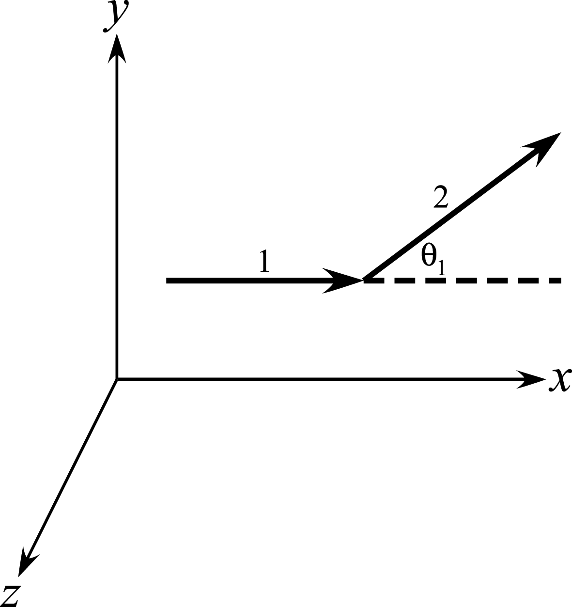
Figure 1. Illustration of magnetic-field alignment change altering the course of electrons.
Since our focus is the partitioning of kinetic energy, the magnitude of the magnetic field is unimportant as long as its variation near the discontinuity is negligible; if this is not the case, then adiabatic invariants can be incorporated to describe the variation of the perpendicular component of the kinetic energy away from the intersection points of different field lines, which we will not perform here (Bellan Reference Bellan2008; Chen Reference Chen2012). For convenience, we shall rotate our coordinate system so that the  $x$-axis is aligned with the original local magnetic field. The $y$-axis will be defined so that the new magnetic-field line that is encountered resides in the $x$–
$x$– $y$ plane; the $z$-axis is perpendicular to the plane formed by the two field lines. The angle by which the new magnetic field departs from the previous one is defined by $\unicode[STIX]{x1D703}_{1}>0$. We have employed the labels ‘1’ and ‘2’ to designate in the figure the first and second magnetic-field lines encountered by the particle. It is convenient to decompose at any time the motion into parallel (i.e. along $\boldsymbol{B}$) and perpendicular parts, with associated velocities $v_{\Vert }$ and $v_{\bot }$ respectively. We expect that the electrons will gyrate around the relevant field line and that the velocity and position of the electron will vary continuously as it transitions from one field line to the next.
For the first field line, we will regard  $v_{x}=v_{\Vert }$ as being constant. Similarly, we will regard $v_{y}=v_{\bot }\,\cos \unicode[STIX]{x1D711}$ and $v_{z}=v_{\bot }\,\sin \unicode[STIX]{x1D711}$ as being the velocity of the electron with respect to the $y$-axis and $z$-axis, respectively, where $\unicode[STIX]{x1D711}$ describes the angle of gyration executed by the charged particle around the $x$-axis. We will presume that $\unicode[STIX]{x1D711}$ varies linearly in time; we will be performing angle or, equivalently, time averages over quantities $\cdots$ designated $\langle \cdots \rangle$ over $\unicode[STIX]{x1D711}$ to calculate their average effect. For the second field line, we must convert our coordinates to ones associated with the now-changed magnetic-field geometry, and this therefore requires a rotation of coordinates. Our new $x$-axis, which we will refer to as $x^{\prime }$, is aligned with the new field whose orientation has rotated in the $x$–
$x$– $y$ plane by $\unicode[STIX]{x1D703}_{1}$. Similarly, our new $y$-axis has rotated by $\unicode[STIX]{x1D703}_{1}$ to $y^{\prime }$ while the $z$-axis remains unchanged as $z^{\prime }$. Therefore, we can immediately write
 $$\begin{eqnarray}\left.\begin{array}{@{}c@{}}\displaystyle v_{x^{\prime }}=+v_{x}\,\cos \unicode[STIX]{x1D703}_{1}+v_{y}\,\sin \unicode[STIX]{x1D703}_{1}\\[5.0pt] \displaystyle v_{y^{\prime }}=-v_{x}\,\sin \unicode[STIX]{x1D703}_{1}+v_{y}\,\cos \unicode[STIX]{x1D703}_{1}\\[5.0pt] \displaystyle v_{z^{\prime }}=v_{z}.\end{array}\right\}\end{eqnarray}$$
Further, we observe that
 $$\begin{eqnarray}\left.\begin{array}{@{}c@{}}\displaystyle v_{x}=v_{\Vert }\\[5.0pt] \displaystyle v_{y}=v_{\bot }\,\cos \unicode[STIX]{x1D711}\\[5.0pt] \displaystyle v_{z}=v_{\bot }\,\sin \unicode[STIX]{x1D711},\end{array}\right\}\end{eqnarray}$$
 where  $\unicode[STIX]{x1D711}$ is the gyration angle which can be regarded as a uniformly distributed random variable.
In analogy to Brownian motion described in §2, we average over the assumed uniformly distributed gyration angle  $\unicode[STIX]{x1D711}$ and observe that
 $$\begin{eqnarray}\left.\begin{array}{@{}c@{}}\displaystyle \left\langle v_{y}\right\rangle =0\\[5.0pt] \displaystyle \left\langle v_{z}\right\rangle =0\\[5.0pt] \displaystyle \left\langle v_{x}\right\rangle =v_{\Vert },\end{array}\right\}\end{eqnarray}$$
analogous to the ‘guiding centre’ approximation in plasma physics.
Corresponding with conventional Brownian motion, averages over many quantities simply disappear, but averages over quadratic quantities do not. We observe that
 $$\begin{eqnarray}{\textstyle \frac{1}{2}}=\left\langle \sin ^{2}\unicode[STIX]{x1D711}\right\rangle =\left\langle \cos ^{2}\unicode[STIX]{x1D711}\right\rangle .\end{eqnarray}$$
Therefore, we are able to write
 $$\begin{eqnarray}\left.\begin{array}{@{}c@{}}\displaystyle \left\langle v_{x^{\prime }}^{2}\right\rangle =\left\langle v_{\Vert }^{\prime 2}\right\rangle =\left\langle v_{\Vert }^{2}\right\rangle \,\cos ^{2}\unicode[STIX]{x1D703}_{1}+{\textstyle \frac{1}{2}}\,\left\langle v_{\bot }^{2}\right\rangle \,\sin ^{2}\unicode[STIX]{x1D703}_{1}\\[5.0pt] \displaystyle \left\langle v_{y^{\prime }}^{2}\right\rangle =\left\langle v_{\Vert }^{2}\right\rangle \,\sin ^{2}\unicode[STIX]{x1D703}_{1}+{\textstyle \frac{1}{2}}\,\left\langle v_{\bot }^{2}\right\rangle \,\cos ^{2}\unicode[STIX]{x1D703}_{1}\\[5.0pt] \displaystyle \left\langle v_{z^{\prime }}^{2}\right\rangle =\left\langle v_{z}^{2}\right\rangle ={\textstyle \frac{1}{2}}\left\langle v_{\bot }^{2}\right\rangle \end{array}\right\}\end{eqnarray}$$
from which we obtain
 $$\begin{eqnarray}\displaystyle \left\langle v_{\bot }^{\prime 2}\right\rangle & = & \displaystyle \left\langle v_{y^{\prime }}^{2}\right\rangle +\left\langle v_{z^{\prime }}^{2}\right\rangle \nonumber\\ \displaystyle & = & \displaystyle \left\langle v_{\Vert }^{2}\right\rangle \,\sin ^{2}\unicode[STIX]{x1D703}_{1}+{\textstyle \frac{1}{2}}\,\left(1+\cos ^{2}\unicode[STIX]{x1D703}_{1}\right)\left\langle v_{\bot }^{2}\right\rangle .\end{eqnarray}$$
We can now combine these expressions in matrix form
 $$\begin{eqnarray}\left[\begin{array}{@{}c@{}}\left\langle v_{\Vert }^{\prime 2}\right\rangle \\[5.0pt] \left\langle v_{\bot }^{\prime 2}\right\rangle \end{array}\right]=\left[\begin{array}{@{}cc@{}}\cos ^{2}\unicode[STIX]{x1D703}_{1} & {\textstyle \frac{1}{2}}\,\sin ^{2}\unicode[STIX]{x1D703}_{1}\\[5.0pt] \sin ^{2}\unicode[STIX]{x1D703}_{1} & {\textstyle \frac{1}{2}}+{\textstyle \frac{1}{2}}\cos ^{2}\unicode[STIX]{x1D703}_{1}\end{array}\right]\,\left[\begin{array}{@{}c@{}}\left\langle v_{\Vert }^{2}\right\rangle \\[5.0pt] \left\langle v_{\bot }^{2}\right\rangle \end{array}\right].\end{eqnarray}$$
 We will refer to the matrix involving the field deflection angle  $\unicode[STIX]{x1D703}_{1}$ as $\unicode[STIX]{x1D648}(\unicode[STIX]{x1D703}_{1})$. Suppose that we have many such scatterings designated by the subscript $n$ with angles $\unicode[STIX]{x1D703}_{1}$, $\unicode[STIX]{x1D703}_{2},\ldots ,\unicode[STIX]{x1D703}_{n}$. Then, we must address the composition of the matrices via the matrix product $\unicode[STIX]{x1D648}(\unicode[STIX]{x1D703}_{n})\boldsymbol{\cdot }\unicode[STIX]{x1D648}(\unicode[STIX]{x1D703}_{n-1})\cdots \unicode[STIX]{x1D648}(\unicode[STIX]{x1D703}_{2})\boldsymbol{\cdot }\unicode[STIX]{x1D648}(\unicode[STIX]{x1D703}_{1})$. In order to accomplish this objective, we must solve the associated eigenvalue problem, taking note that the matrices $\unicode[STIX]{x1D648}$ are neither symmetric nor Hermitian.
4 Diagonalization properties
Insight into the eigenvalue problem can be obtained using physical intuition. Since the kinetic energy per unit mass  ${\mathcal{E}}$ is conserved by the Lorentz equation, we verify that
 $$\begin{eqnarray}{\mathcal{E}}\equiv {\textstyle \frac{1}{2}}\left[\left\langle v_{\Vert }^{2}\right\rangle +\left\langle v_{\bot }^{2}\right\rangle \right]\end{eqnarray}$$
is preserved therefore establishing that the associated eigenvalue is 1, implying that the energy does not change. To identify the other eigenvector, we recall that
 $$\begin{eqnarray}\left\langle v_{y}^{2}\right\rangle =\left\langle v_{z}^{2}\right\rangle ,\end{eqnarray}$$
establishing equipartition of energy in the two perpendicular dimensions. If the energy were fully isotropic, we would expect to have
 $$\begin{eqnarray}\left\langle v_{\Vert }^{2}\right\rangle ={\textstyle \frac{1}{2}}\left\langle v_{\bot }^{2}\right\rangle .\end{eqnarray}$$
 Accordingly, we will define  ${\mathcal{A}}$ as a measure of anisotropy, namely
 $$\begin{eqnarray}{\mathcal{A}}=\left\langle v_{\Vert }^{2}\right\rangle -{\textstyle \frac{1}{2}}\,\left\langle v_{\bot }^{2}\right\rangle .\end{eqnarray}$$
Thus, employing eigenvalue form, we observe from (3.8) that
 $$\begin{eqnarray}\left[\begin{array}{@{}c@{}}{\mathcal{E}}^{\prime }\\[2.0pt] {\mathcal{A}}^{\prime }\end{array}\right]=\left[\begin{array}{@{}ccc@{}}1 & \quad & 0\\[2.0pt] 0 & \quad & 1-{\textstyle \frac{3}{2}}\,\sin ^{2}\unicode[STIX]{x1D703}_{1}\end{array}\right]\,\left[\begin{array}{@{}c@{}}{\mathcal{E}}\\[2.0pt] {\mathcal{A}}\end{array}\right].\end{eqnarray}$$
 We note that the eigenvalue associated with  ${\mathcal{A}}$, namely $1-(3/2)\,\sin ^{2}\unicode[STIX]{x1D703}_{1}$, can be positive or negative, depending upon the angle of deflection by which the electrons are diverted from one field line to another. The eigenvalue ${\mathcal{A}}$ becomes as large as 1, for the case of no deflections, and can be as small as $-1/2$, if all of the energy in the electron has gone into gyromotion. Importantly, however, the eigenvalue ${\mathcal{A}}$ is always less than 1 in magnitude, thus assuring that the degree of anisotropy is invariably decreasing. In the language of nonlinear dynamics, this mapping and the ensuing isotropization is a global attractor.
5 Summary and conclusion
The eigenvalue properties derived above guarantees that the outcome of many magnetic-field deflections results in a dramatic reduction of anisotropy. An isotropic velocity distribution can be expected to emerge rather quickly, paralleling the isotropization that occurs in collisional environments akin to Brownian motion. Charged particle observations in various space and astrophysical environments complicate matters. Since observational footprints typically encompass large spatial regions, we should consider sub-regions where field strengths and orientations are relatively smoothly varying as well as smaller sub-regions characterized by substantial fluctuations in field orientations. Thus, if electrons appear to be highly collimated in a localized region where field line orientations could be disordered, it follows that there must be a source for particle collimation or energization. Finally, returning to the conventional wisdom that collisionless plasmas cannot become isotropic, we have shown that particle motion in highly complex field environments such as those possibly found in regions of tortuous, turbulent, tangled fields could generate isotropic behaviour arising from ‘kinks’. A simple way to understand this is to take note that charged particle motion here can undergo sharp deflections, just as they would in collisional environments, owing to highly complicated field structures and the ‘kinks’ that they present. Turbulent magnetic fields, under the right circumstances, can become a proxy for particle collisions.
Acknowledgements
The author is especially grateful for comments and suggestions made by N. Hamlin, as well as by J. Rudnick, V. Angelopoulos, M. Kivelson, Y. Rephaeli and R. Lovelace which helped improve the verisimilitude and clarity of the model. The author is also grateful to the reviewers who identified elements of the narrative which could be clarified. W.I.N. thanks the Institute for Advanced Study in Princeton for its hospitality during my sabbatical year away from the University of California, Los Angeles, and for funding as IBM Einstein Foundation Fellow at the Institute during the 2018–2019 academic year.
Editor Troy Carter thanks the referees for their advice in evaluating this article.

