


Introduction
The consultants responsible for avalanche path analysis must answer the following questions: Is there any avalanche hazard on the path? Which kinds of avalanche can occur? In which conditions? What are the properties of these avalanches (magnitude, velocity, extension, pressure fields, etc.)? These analyses will give the basic information to recommend the best protection strategy (Reference Buisson and CharlierBuisson and Charlier, 1989).
The consultants have several tools to analyse an avalanche path. First of all, they can use their experience. They can make comparisons between a particular avalanche path and some other well-known paths. They can make assumptions based on terrain and vegetation features. But more and more, in avalanche hazard zoning, velocity and run-out distance are required for building design. Snow specialists can use simulation methods based on mechanical equations. Numerous models have been developed from Voellmy’s model mainly to describe a flowing avalanche (Reference Bakkehøi, Cheng, Domaas, Lied, Perla and SchieldropBakkehøi and others, 1981; Reference Beghin and BrugnotBeghin and Brugnot, 1983; Reference Brugnot and VilaBrugnot and Vila, 1985; Reference Norem, Irgens and SchieldropNorem and others, 1989; Reference Salm, Burkard and GublerSalm and others, 1990; Reference MartinetMartinet, 1992; Brandstätter and others, unpublished).
ELSA is a computer tool dedicated to avalanche path analysis (Reference Buisson and CharlierBuisson and Charlier, 1989). It tries to provide not only some of these numerical simulation methods, but also some empirical methods developed by using the experience of avalanche experts. These methods provide input data for the numerical models. Recent develop-ments in computer science enable the knowledge of avalanche experts to be captured. Symbolic models based on this knowledge can then be implemented (Reference BuissonBuisson, 1990a).
There is no conflict between these two kinds of method. They are complementary and can be combined to produce an improved output.
Description of Terrain
ELSA must be provided with an accurate description of terrain, which plays an important part in avalanche path analysis. Topography, vegetation and the nature of the soil surface are the parameters which, in combination with meteorological conditions, control the release and flow behaviour of avalanches. In numerical models, the terrain profiles are used to describe the geometry of the avalanche track. The vegetation and the the soil surface are important in the choice of roughness coefficients. In symbolic models, slope, topography around the ridges, and exposure to prevailing wind direction are used as determinants for the computation of snowdrift, snow cover stability and fracture propagation.
Three zones
The different models available in ELSA cannot be used on the whole avalanche path. As a result, we assume that the user is able to define the starting zone, the avalanche track, and the run-out zone clearly (Fig. 1). This decomposition is common. The starting zone is that part of the terrain where the mass of snow which will be involved in the avalanche is released. The fracture propagation and the acceleration of the avalanche are principal features of this zone. The avalanche track is where the avalanche simply flows and the run-out zone is where the avalanche decelerates and finally stops.
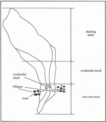
Fig. 1. The Drayre avalanche path in Vaujany, Isère, Région Rhône-Alpes, France.
Triangles and topography
In order to describe the topography mathematically, a digital terrain model (DTM) is required. A triangulation method is used which describes the natural terrain as planar triangles (Fig. 2) with each triangle defined by the coordinates of its vertices. This method was suggested by Toppe (personal communication) in order to keep the number of triangles low and to get an accurate DTM adapted to the terrain features.
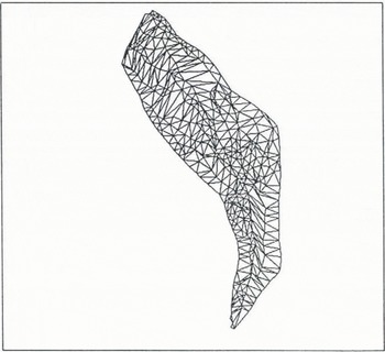
Fig. 2. Triangulation analysis for the Drayre avalanche path.
Panels
The same symbolic models are based on experts’ knowledge. As a result, ELSA must use the same terrain analysis methodology as these experts do. The experts do not reason in small triangles; instead, they use a unit of terrain called a panel. A panel is considered to be homogeneous according to the criteria of the avalanche path analysis: slope, exposure, vegetation, soil and distance to the main ridges. Panels are represented in ELSA as polygons defined by the union of several connected triangles. The panel represents the minimum topological decomposition of the terrain (Fig. 3). ELSA does not consider units of terrain which are less than the size of a panel.
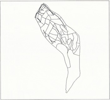
Fig. 3. Simplification of the Drayre avalanche path into panels. Ridges and breaks of slope are represented by lines.
A construction system
The triangle and panel specifications suggest the process of their construction. The basic idea is to use the data which are easily obtained from sources such as (1) contour line maps, (2) ridges and breaks of slope maps, (3) singularity line maps (showing changes in aspect, gullies, furrows, etc.), and (4) vegetation and soil surface maps. All of these polygonal lines will become constraints in the building of triangles: i.e. these lines cannot cut through a triangle.
According to the specifications of the panels, these polygonal lines may have several meanings. Some must be panel boundaries (e.g. vegetation or ridge line); others may be included in the interior of a panel (a contour line for instance). In this latter case, the lines are used only for the construction of the triangles.
The terrain construction system is based on polygonal lines. Each vertex of these lines must be known through its three coordinates. If x and y are defined through the digitization of the map, the z-coordinates can be provided only by the contour line map. As a consequence, we decided not to work with the initial data maps (2), (3) and (4) (Fig. 4a) but with the lines defined by the intersection of these data with the contour lines from map (1) (Fig. 4b). Naturally, the user is allowed to keep one particular point on a line of maps (2), (3) and (4) but he must provide the elevation of this point (Fig. 4c).
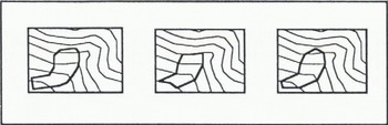
Fig. 4. a, b and c: polygonal lines used in the construction.
The contour lines maps are purchased at l’Institut Géographique National which is in charge of mapping in France. The available digitized contour lines are adapted to a scale of 1 :10 000. The other maps (2), (3) and (4) are digitized by the user on the graphic interface of ELSA. This operation requires a good analysis of the natural terrain.
Meteorological Conditions
An avalanche occurs when a particular scenario takes place on an avalanche path.
A scenario is described through an initial condition and a sequence of events. An initial condition defines the distribution of the snow in the starting zone. The last event is called the critical event and it ends with an avalanche release.
ELSA is able to deal with two scenarios:
a heavy snowfall on an existing snow cover triggers an avalanche; a snowfall on an existing snow cover creates a new snow cover and an artificial release is triggered later on a panel.
In both scenarios, the snowfall event can occur with or without snowdrift. The user can choose the wind direction and the empirical level of snowdrift. The user can also choose the character of the snow available for avalanche (e.g. the new snow from a snowfall) in both scenarios. The character is defined by physical parameters: density, cohesion, friction angle. The existing snow cover (called the old snow) in the initial condition is not supposed to contribute mass to the avalanche but is described by its upper surface (the sliding surface). The initial condition provides a distribution of snow heights.
Modelling Several Phenomena
During an avalanche, several phenomena take place in the avalanche path as shown in Figure 5. Four phenomena are analyzed: snowdrift, snow cover stability, release propagation and avalanche flow and stopping. The first three are located mainly on the starting zone, the last on the avalanche track and on the run-out zone.
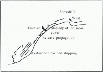
Fig.5. Avalanche phenomena taken into account by ELSA.
Snowdrift
Snowdrift and its influence on avalanches have been studied both theoretically and experimentally (Reference Föhn and MeisterFöhn and Meister, 1983; Reference MeisterMeister, 1989). In ELSA a symbolic simulation of snowdrift is based on empirical knowledge. The first assumption is that the spatial analysis of panels is relevant and yields homogeneous units with reference to this phenomenon. Several parameters are used to estimate snowdrift on each panel: relative position of the panel to the ridge (Fig. 6); shape of the ridge (assumed to be symmetric); distance to the ridge; incidence angle between the wind and the ridge; and position of the panel and the ridge relative to wind (lee- or windward). The result of the snowdrift analysis is an empirical distribution of a coefficient between 0 and 5. A coefficient of 1 means that snowdrift has no effect. A coefficient less than 1 means that there is wind erosion; a coefficient greater than 1 means that there is wind deposit. The limit of 5 is the maximum value.
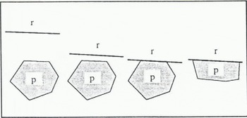
Fig.6. Four relative positions between a ridge, r, and a panel, p, considered by ELSA: near, very near, juxtaposed and on.
Snow cover stability
Two methods are used in order to estimate the snow cover stability. This stability is then used in the analysis of release propagation. The first one is based on a single rule: if the upper snow layer is a slab (i.e. with a good cohesion) and if it lies on a weak layer with no cohesion or a sliding surface without anchorage, the stability depends only on the relative values of the slope angle i and the external friction angle ϕ As a result, the stability condition is ϕ≥i
If this condition is not true, we consider that the upper snow layer is held by its lateral anchorage. This will explain the fracture propagation.
Another very simple model is used in the starting zone to calculate the stability. It is based on the soil mechanics interpretation which gives, for a homogeneous material and an infinite domain, the critical depth hcrit (measured vertically) of material above which a slide can appear:
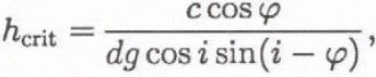
where g is acceleration due to gravity, i is slope angle, d is density of the material (in this case, the upper snow layer), c is cohesion of the material, and ϕ is internal friction angle of the material.
In this case, the condition for stability is hcrit≥h.
If h > hcrit , the upper snow layer is considered to be unstable. In both cases, if there is a release, the whole unstable snow layer is considered to be involved.
For both methods, we take into account the mean particle size at the soil surface. For example, in a slope covered with scree (size 0.5 m), we assume that no slide can occur in the layer between 0 and 0.5 m. In other words, the snow which smoothes the terrain is not taken into account for the calculation of stability (Fig. 7). We use the same approach for grass, bushes and small trees. For forests and large trees, we use an arbitrary association between types of tree cover and size of screes. In determining this slide surface, we also take into account the old snow described in the initial condition of the scenario. Therefore, in this paper, we speak of the efficient snow height, that is, the height of the snow which can slide.
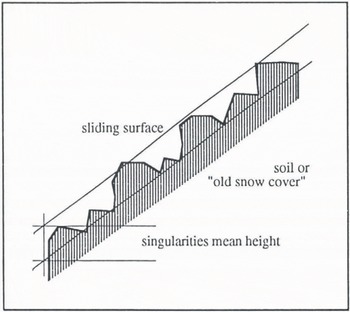
Fig.7. The sliding surface on a natural terrain.
Also, in ELSA the user is always allowed to control the stability in a particular panel.
Release propagation
In the release propagation, two phenomena occur with different characteristic times. The faster is a wave propagation which takes place in a cohesive snow layer where the slab stability condition is exceeded; it is the fracture propagation. The slower is the gradual entrainment of snow masses moving down slope and is called movement propagation. These two phenomena act together to determine the part of the starting zone released (Fig. 8).
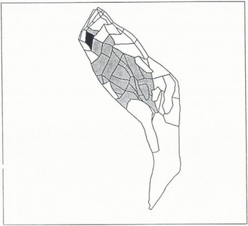
Fig.8. An example of release in the Drayre avalanche path. The panel in black is considered to be the trigger. The shaded panels are considered to be released.
The wave-like fracture propagation is based only on the stability inferred according to the first method (slab stability). If a panel p1 is seen as unsteady according to this method, then it is released as soon as a neighbour, p2, is released.
The second phenomenon is dealt with by exploiting another simple model. A panel p2 with an area Σ2 was not released by the first propagation phenomenon; i.e. there was no slab or weak layer. Moreover, the snow height h2 was lower than the critical snow height h2c. A volume of Ω 1 of snow arrives on p2. If it is large enough to overload p2, there is propagation. This condition is
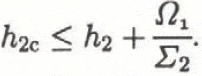
When the condition is not fulfilled, we consider that the propagation has stopped.
The character of the snow plays a large part in the computation of h2c . We assume that the character of the movable snow and the moving snow are the same everywhere. The spatial analysis of panels plays a large part in this model.
Avalanche flow
As explained above, the avalanche motion can be simulated by several methods, but only two of them are available in ELSA: the method presented by Reference Bakkehøi, Cheng, Domaas, Lied, Perla and SchieldropBakkehøi and others (1981, modified from the Voellmy’s method) and the Saint-Venant’s model solved by the numerical scheme created by Reference Brugnot and VilaVila (1984) and developed by Reference MartinetMartinet (1992).
The first method requires an estimation of the mass of snow involved in the avalanche. The second method requires a hydrograph, i.e. a flow rate versus time at the beginning of the avalanche track. The mass is given by the analysis of the fracture propagation. The user must choose a flow time.
Integration
Integration is used here to mean the introduction and the articulation of several methods in the same computer system.
This paper presents several methods used in ELSA. Some methods have been used already (especially the last ones, dedicated to avalanche flow); some are new and need more work to be validated. These methods are integrated in ELSA. The knowledge-based system architecture allows for the development of problem solving environments (Buisson, 1990b).
ELSA is built on an object-oriented knowledge representation system, SHIRKA (Rechenmann and others, unpublished), which is written in Le-Lisp, a Lisp dialect (Reference IlogIlog S.A., 1991). ELSA runs on a SUN IPC workstation with UNIX.
Sharing data
One of ELSA’s main strengths is the sharing of data between several methods. The best example is topography. All the different methods use triangulation to represent terrain. However, the first three methods make intensive use of the decomposition in panels. The main advantage of data sharing lies in consistency and in time saving.
Cooperation
The output of the symbolic simulation can drive the numerical simulation and vice versa. As a result, all the phenomena described above are linked to one another in the analysis.
Interactive interface
The interactive interface allows non-computer specialists to use ELSA. The user-friendly colour interface based on a mouse and a high definition screen highlights the important parameters. The keyboard of the workstation is hardly used and the user does not need to know or use the computer operating system or programming languages.
The language Le-Lisp is provided with Aïda, an object-oriented environment for the development of graphic applications (Reference IlogIlog S.A., 1992). The figures in this paper come from the interface. It is used for the construction process (definition of the lines presented in Figure 4a) and for the presentation of results: snow heights map, stability distribution, initial fracture location and release propagation. The scenarios are also displayed in a graphic representation.
Future Developments
ELSA is still being developed. Besides the capabilities presented in this paper and which have already been implemented, further developments are being considered: terrain validation of some methods; further analysis of stability in a forested or tree-covered area; integration of the AVAER (AValanche AERosol) program for aerosol avalanches (Rapin, unpublished); and integration of a statistical method for the estimation of the run-out distance such as described by Reference Bakkehøi, Cheng, Domaas, Lied, Perla and SchieldropBakkehøi and others (1981).
Acknowledgements
This research has been supported by grants from La Région Rhône-Alpes in 1989 and 1990 and from La Délégation aux Risques Majeurs (Ministère de l’Environnement) in 1990 and 1991.
We would like to thank Harald Norem from NGI in Oslo, Norway, Ronald Toppe, formerly from NGI, and Hansueli Gubler from IFENA in Davos, Switzerland, for their relevant advice.


