


Introduction
Agriculture in developing countries needs to transform and increase food production by about 70% to meet demand by 2050 (FAO, 2010; Tilman et al., Reference Tilman, Balzer, Hill and Befort2011). Food security in Africa is a priority due to a high population growth rate coupled with some unfavourable biophysical conditions, socio-economic developments and political issues. This includes poor soils, adverse climates, a heavy burden of pests and diseases and inadequate agricultural infrastructure (Gatzweiler and von Braun, Reference Gatzweiler and von Braun2016). Gbetibouo et al. (Reference Gbetibouo, Ringler and Hassan2010) pointed out that smallholders dependent on rainfed agriculture and a high degree of soil degradation are the most vulnerable.
With regard to crop production in South Africa (SA), maize is the most important staple crop and mostly grown under rainfed conditions. The yield of maize in the Limpopo province is fairly low – for smallholder farmers ranging between 1 and 2 t/ha. This is mainly due to manual farming techniques together with low input provision such as no or little fertilizer application, lack of quality seeds and no irrigation (FAO, 2010). The increase in water scarcity and land degradation, particularly poor soil fertility in most smallholder farming systems poses a serious threat to crop production in SA. Therefore, a logical agricultural intervention measure is to increase crop yield per volume of water used and replenish the nutrient-depleted soils with mineral and organic fertilizer. Water use efficiency (WUE) is mentioned in this research aiming at finding appropriate technological improvements and innovations to support sustainable agricultural productivity. Saving water and promoting crop growth through appropriate fertilization could be an effective measure to maximize WUE. Regarding semi-arid areas, a shortage of soil moisture during the growing stage of the crop often results in poor crop growth and low grain yield. Therefore, applying deficit irrigation during crop growing stages can improve yield and WUE. Several studies have indicated that applying irrigation measures increases WUE in maize (Hernández et al., Reference Hernández, Echarte, Della Maggiora, Cambareri, Barbieri and Cerrudo2015; Kresovic et al., Reference Kresovic, Tapanarova, Tomic, Zivoti, Vujovic, Sredojevic and Gajic2016). Sadras et al. (Reference Sadras, Grassini and Steduto2012) reported an increase in WUE values from 1.1–3.2 kg/m3 for irrigated maize to 0.6–2.3 kg/m3 for rainfed maize. In addition, application of nitrogen in environments with adequate rainfall or soil moisture availability can increase WUE in maize (Hernández et al., Reference Hernández, Echarte, Della Maggiora, Cambareri, Barbieri and Cerrudo2015; Zhang et al., Reference Zhang, Dai, Ma, Fan, Meng, Han and Liao2022).
Dynamic crop simulation models (CSMs) that are often embedded in crop modelling platforms with software packages for input and output handling and their visualization, such as Decision Support System for Agrotechnology Transfer (DSSAT) (Hoogenboom et al., Reference Hoogenboom, Porter, Boote, Shelia, Wilkens, Singh, White, Asseng, Lizaso, Moreno, Pavan, Ogoshi, Hunt, Tsuji, Jones and Boote2019a), Agricultural Production Systems Simulator (APSIM) (Holzworth et al., Reference Holzworth, Neil, Peter, Eric, Neville, Greg and Karine2014), Root Zone Water Quality Model (RZWQM2) (Ma et al., Reference Ma, Ahuja, Nolan, Malone, Trout and Qi2012), Environmental Policy Integrated Climate (EPIC) (Williams, Reference Williams, Jones, Kiniry and Spanel1989), World Food Studie (WOFOST) (Supit et al., Reference Supit, Hooijer and Van Diepen1994) and others, can be useful tools for simulating crop growth and yield formation for different genotype (G) × environment (E) × management (M) combinations (Rötter et al., Reference Rötter, Van Keulen and Jansen1997, Reference Rötter, Tao, Höhn and Palosuo2015; Liu et al., Reference Liu, Yang, Drury, Reynolds, Tan, Bai, He, Jin and Hoogenboom2011; Yan et al., Reference Yan, Xiying, Muhammad, Hongjun, Haichun and Zvi2020). In recent years, DSSAT has been used widely to predict nitrogen dynamics, crop yield and water use of a whole range of crops and cropping systems (Jones et al., Reference Jones, Hoogenboom, Porter, Boote, Batchelor, Hunt, Wilkens, Singh, Gijsman and Ritchie2003; Thornton et al., Reference Thornton, Jones, Alagarswamy and Andresen2009; Liu et al., Reference Liu, Yang, Drury, Reynolds, Tan, Bai, He, Jin and Hoogenboom2011; Hoogenboom et al., Reference Hoogenboom, Porter, Boote, Shelia, Wilkens, Singh, White, Asseng, Lizaso, Moreno, Pavan, Ogoshi, Hunt, Tsuji, Jones and Boote2019a). CSMs have sound algorithms for describing the main processes of crop growth and development in dependence of given environmental (soil and climate) conditions and for predicting the effects of alternative management options, such as best management practices (BMPs) for nutrients and water on yield formation at the field scale. Their input data requirements are accordingly high. However, the usage of CSMs at catchment scale is rather limited and often difficult, especially in hilly areas with great variability of soils, slope and land use. Agro-hydrological models (AHMs), such as Soil and Water Assessment Tool (SWAT) (Arnold et al., Reference Arnold, Srinivasan, Muttiah and Williams1998), Système Hydrologique Europée (MIKE SHE) (Refsgaard and Storm, Reference Refsgaard, Storm and Singh1995) or Agricultural Policy/Environmental Extender (APEX) (Gassman et al., Reference Gassman, Williams, Wang, Saleh, Osei, Hauck, Izaurralde and Flowers2010), can be considered as the suitable tools to investigate the effects of BMPs on crop performance under different environmental conditions in a catchment. The SWAT model has been widely used to simulate the impact of land-management practices on water, nutrient transport and agricultural productivity in watersheds with varying soil, land-use, climate and management conditions (Tripathi et al., Reference Tripathi, Panda, Raghuwanshi and Singh2004; Lam et al., Reference Lam, Schmalz and Fohrer2011; Nair et al., Reference Nair, King, Witter, Sohngen and Fausey2011; Sinnathamby et al., Reference Sinnathamby, Douglas-Mankin and Craige2017). The key strength of SWAT is a flexible framework that allows prediction of many types of BMPs such as application rate and timing of fertilizers and irrigation, cover crops (Gassman et al., Reference Gassman, Reyes, Green and Arnold2007). However, the crop growth model in SWAT is based on a simplification of the EPIC crop model (Williams et al., Reference Williams, Jones and Dyke1984), which has a low capability to accurately predict crop yield for different G × E × M combinations and is much less suitable for that than the DSSAT model under similar study area conditions (Dechmi et al., Reference Dechmi, Playan, Faci and Cavero2010). In addition, several studies have identified that the auto-irrigation functions in SWAT did not adequately represent field practices (Chen et al., Reference Chen, Gary, Marek, Thomas, Marek, Brauer and Srinivasan2017). These limitations of the models urge for another approach, which is a coupling and combining the strengths and functionalities of different models like SWAT and DSSAT. This approach can be expected to be a suitable solution for assessing the effects of agricultural management practices on crop productivity in a watershed. To date, various CSMs that can describe major crop growth processes in interactions with environment and management have been integrated successfully with hydrological models. Examples of just coupling includes DSSAT–RZWQM (Ma et al., Reference Ma, Hoogenboom, Ahuja, Ascough and Saseendran2006), DSSAT– Soil Water Atmosphere Plant (SWAP) (Dokoohaki et al., Reference Dokoohaki, Gheysari, Mousavi, Zand-–Parsa, Miguez, Archontoulis and Hoogenboom2016), WOFOST–WEP (Jia et al., Reference Jia, Shen, Niu, Qiu, Wang and Liu2011) and EPIC–SWAT (Zhang et al., Reference Zhang, Shao, Ye and Xing2014). For example, Jia et al. (Reference Jia, Shen, Niu, Qiu, Wang and Liu2011) used water and moisture availability obtained from the Water and Energy Transfer Processes (WEP) model as input data for the WOFOST model. In the current study, the approach we aimed to couple the model DSSAT with SWAT. In this approach, the DSSAT model is used to determine crop water requirements and then feeds the data to the SWAT model. With this approach, it is possible to determine the water stress levels associated with different variants of crop–climate–agricultural management combinations for a given watershed.
The present study aimed to: (1) operationalize the coupling of DSSAT–SWAT model to simulate soil water dynamics, maize growth and yield from field to catchment scale, (2) evaluate the effects of a number of BMPs on maize yield, water use and WUE, and (3) assess the spatial variation of yield and to identify the best agricultural management interventions to narrow yield gaps under current climatic conditions of the study area.
Materials and methods
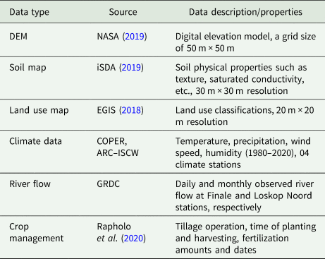
Study area description and data collection
The study areas are mainly located in the Limpopo province, SA. The rainy season is characterized by hot and humid conditions occurring during summer months (October–April). Dry winters (May–September) are warm and mild but cold at night (Fig. 1). The field trials represent different climatic conditions (see, Fig. 1). The first site is Syferkuil, the experimental farm of the University of Limpopo (23°50’10”S latitude, 29°41’34”E longitude, and 1250 m elevation above mean sea level) can be characterized as a semi-arid upland site. The second site, the experimental farm of the University of Venda, is Univen (22°58’49”S latitude, 30°26’16”E longitude, and 712 m elevation above mean sea level) can be characterized as sub-humid, warm midland site. Average rainfall at the Syferkuil and Univen stations are 485 and 820 mm, respectively, during the growing season from November to April.

Figure 1. Average monthly total precipitation, maximum and minimum air temperature over the period 1985–2020 for (a) Syferkuil and (b) Univen site.
Soil data of the experimental sites
Soil at Syferkuil is a sandy clay loam, characterized by its high sand content (57–58%). Clay content ranges from 25 to 29% at different soil layers. At Univen, soil is a sandy loam, containing relatively high sand content up to 72%, while clay content only accounts for 14–16% (Table 1). The 0–90 cm soil layer had on average total nitrogen levels of 0.96 and 0.65 g/kg for the Syferkuil and Univen site, respectively.
Table 1. Soil properties up to a maximum rooting depth for the Syferkuil and Univen sites

CLL is crop lower limit. DUL is the drained upper limit.
Agronomic field experiments and survey data
The agronomic experiments were set up in a randomized complete block design with three replicates at each research site, Syferkuil and Univen. Only sole-maize cultivar Hybrid PAN 6479 was grown for the experiment. The size of the experimental plot is 4.5 m × 4 m. Maize was sown using intra-row spacing of 90 cm with the density of three plants/m2. The experiments were carried out in two separate seasons. Maize was planted on 29 November 2015 for the first season 2015/2016 and on 03 January 2017 for the second season 2016/2017 in Syferkuil, while the planting date for maize was 24 October 2016 for the season 2016/2017 at Univen, while season 2015/2016 failed due to insect damage. The rate of fertilizer application is 40N:30P. Maize grain yield, dry matter at flowering and harvesting time, and soil water content (SWC) were measured during the growing period.
Additional surveys on maize yield were conducted in 2018/2019 in the neighbouring villages Mafarana and Gavaza (Fig. 2 denotes Mafarana only), Limpopo province by the Institute of Tropical Plant Production and Agricultural Systems Modelling, University of Goettingen, Germany (e.g. May, Reference May2019). The weather conditions in these villages are similar to those at the neighbouring Syferkuil site. A total of 319 samples from smallholders in Mafarana and Gavaza villages were collected at the harvest time. The cultivation of maize in this area is based on rainfed conditions and no fertilizer application.

Gravimetric method was used to measure soil moisture contents. Gravimetric SWC was determined biweekly (a total of nine sampling events) for the layers 0–15, 15–30 and 30–60 cm using a soil auger. Soil samples were collected between plants (within rows) and between rows, bulked together according to depths and subsampled for the determination of soil moisture content. Samples were oven dried at 105°C. Volumetric water content was then calculated by multiplying gravimetric water content by the bulk density. Soil properties of the Syferkuil and Univen sites can be seen in Table 1. Field management data are presented in Table 2.
Table 2. Field management data for the two experimental sites and seasons used for model evaluation

Characterization of the study catchment and weather information
The study catchment that includes the Syferkuil site is located upstream of the Olifants River. The total drainage area of the catchment is about 39 000 km2. Due to the division of the terrain, more than 75% of the catchment area is located within the Limpopo province, while the rest of upstream area (about 25%) of this catchment is located in the neighbouring provinces. The highest and lowest elevations of the catchment are 2114 m and 410 m above sea level, respectively (Fig. 2). There are two hydrological monitoring stations located in the river Olifants and its tributary. The first station, Finale, was installed at the catchment outlet and the second station, Loskop Noord, was installed in the tributary of the river Olifants (Fig. 2). Land use is dominated by rangeland grasses (32.33%), followed by forest evergreen (27.48%) and agricultural land (23.19%) of the total study area. Sandy clay loam (80.87%) is dominant soils, followed by sandy loam (16.69%). The information on land use and soil maps is presented in Fig. 2.
Weather stations at or near the sites provided daily solar radiation, maximum and minimum air temperature and precipitation. For Univen, an on-site weather station and the Makwarela station (6 km from site) were used to provide climate data for the period 1985–2014. The climate data from 2015 to 2020 were obtained from the Venda station, provided by the Agricultural Research Council, SA (ARC–ISCW). At the Syferkuil site, daily weather data were derived from an on-site station for the period 1985–2018. The extended weather data from 2019 to 2020 were obtained from the Ammondale weather station, provided by ARC–ISCW.
At Syferkuil, the maximum temperature ranges from about 20 to 29°C, while the minimum temperature ranges from about 2 to 16°C. The lowest temperature occurs in the months from June to August (Fig. 1(a)). The rainy season runs from October to April with average total monthly precipitation ranges from 35 to 85 mm (Fig. 1(a)). Compared to Syferkuil, the weather at Univen is warmer and more humid (Fig. 1(b)). The distribution of temperature and precipitation over time of the year in the two sites is relatively similar, in general. However, the average monthly total precipitation amount from October to April at the Univen site is higher than that of the Syferkuil site, ranging from 50 to 170 mm (Fig. 1(b)).
Model description
DSSAT model input
The DSSAT is a software application program that comprises CSMs to simulate growth, development and yield as a function of the soil–plant–atmosphere dynamics. In this study, the Cropping System Model (CSM)-CERES–Maize module in DSSAT (version 4.7.5) (Jones et al., Reference Jones, Hoogenboom, Porter, Boote, Batchelor, Hunt, Wilkens, Singh, Gijsman and Ritchie2003; Hoogenboom et al., Reference Hoogenboom, Porter, Shelia, Boote, Singh, White, Hunt, Ogoshi, Lizaso, Koo, Asseng, Singels, Moreno and Jones2019b) was applied to simulate maize growth and yield at the field scale. Main input data of the model consist of daily weather data, soil profile data and crop management. The crop management data of sowing date, harvest date, tillage and fertilizer application rate were taken into account in the model. The initial soil nitrogen was set to be 5 kg/ha. Crop data for maize were obtained from the experimental sites as summarized in Table 2.
DSSAT model calibration and evaluation
The calibration and validation of maize grain yield, total biomass and SWC were performed for the season 2015/2016 and 2016/2017 in the Syferkuil site. The validation of maize grain yield and total biomass was further conducted for the season 2016/2017 in the Univen site. Maize development and yield were calibrated using measured data from the trials.
In this study, the timing and amount of the 40N:30P kg/ha fertilizer rate were set up in the model. Grain yield and phenological stages were taken into account in the calibration of the cultivar coefficients. The predicted phenological stages under the calibrated cultivar coefficients were roughly in the same phenological stages as field crops in this study area. The calibrated model coefficients are presented in Table 3.
Table 3. The calibrated cultivar coefficients of maize (Hybrid PAN 6479) for the experimental field at the Syferkuil using CERES–Maize

SWAT model input
The AHM SWAT (Arnold et al., Reference Arnold, Kiniry, Srinivasan, Williams, Haney and Neitsch2013, version 2012) is a basin scale distributed hydrologic model. It was developed to quantify the impact of land management practices in large, complex catchments. SWAT is a continuous time model, which simulates water, nutrient cycles and crop yield with a daily time step. In the SWAT model, the watershed is divided into sub-basins which are then further subdivided into hydrologic response units (HRUs). Each HRU is assumed to consist of homogeneous land use and soils. Major components of the model include hydrology, weather and agricultural management. The content of all components can be found in Arnold et al. (Reference Arnold, Srinivasan, Muttiah and Williams1998) and Neitsch et al. (Reference Neitsch, Arnold, Kiniry, Williams and King2002).
The potential evapotranspiration (PET) is calculated using a Penman–Monteith method. Crop growth and yield parameters in SWAT model are simulated based on a simplification of EPIC model. The main data described in Table 4 were used to set up the SWAT model. The model was established by dividing the basin into 64 sub-basins and 665 HRUs in this study. Management inputs include sowing date, timing and rate of fertilizer application and harvest date for maize as described in Table 2.
Table 4. Input data used for SWAT model
SWAT model calibration and validation
Maize growth and yield were first manually calibrated and validated for the season 2015/2016 and 2016/2017 at the field scale, respectively. The experimental Syferkuil site is located within HRU60 in the study catchment which combines soil (sandy clay loam) with agricultural land (AGRR). Maize parameters were adjusted until the simulated values of the grain yield and biomass were close to measured values at the HRU60. The parameters used for maize yield calibration process are described in Table 5. Simulated maize yield and total biomass values during the growing season in HRU60 were used for a simple comparison with those calculated by DSSAT with the aim of improving the model accuracy. In addition, survey data collected from different sites in the Mafarana village which are located in HRU6, HRU9, HRU11, HRU12 and HRU14 were used to evaluate the SWAT model.
Table 5. Maize growth parameters for the rainfed conditions used for the SWAT model calibration in the field scale (HRU60)

After maize yield calibration and validation, daily and monthly stream flow was simulated. Based on the hydrological data availability, calibration (1985–1998) and validation (2008–2015) of flow were performed for daily time step using measured data from the Finale gauging station at the catchment outlet (Fig. 2). Additional monthly validation of flow was done for the period from 1984 to 1998 at the Loskop Noord station.
Surface runoff and base flow were calibrated simultaneously during the calibration period. Main parameters adjusted during the flow calibration comprise curve number (CN2), available water capacity (SOL_AWC), soil evaporation compensation factor (ESCO), plant uptake compensation factor (EPCO), groundwater revap coefficient (GW_REVAP) and threshold depth of water in the shallow aquifer (GWQMN). Parameters used for the calibration of flow are described in Table 6.
Table 6. Main controlling parameters of the SWAT model and their optimal values for the Finale stations of the catchment

Coupling input/output from the two models
The approach for ‘coupling models’ in this study is not a hard link but implies that the models interact through their input/output files. DSSAT model uses crop parameters, weather and soil data as input to calculate maize growth and yield. Crop water requirements and rooting depth generated by DSSAT are transferred to SWAT as input data. The amount of crop water demand based on the weather conditions is a critical component used to estimate the water balance of the hydrological model. In this study, the automatic irrigation in the DSSAT model was set at 50% of the available soil moisture, similar to the approach followed by Attia et al. (Reference Attia, Hendawy, Suhaibani, Alotaibi, Tahir and Kamal2021) and Kisekka et al. (Reference Kisekka, Aguilar, Rogers, Holman, O'Brien and Klocke2016). Using crop water demand derived from the DSSAT model as input to the SWAT model can significantly improve predicting water balance components in a watershed, while no observed data on timing and amount of irrigation for maize in local cultivation areas are being collected. Estimated SWCs and evapotranspiration rates by the SWAT model were then compared to those of the DSSAT model using the same datasets at the field scale. In addition, simulated maize yield and biomass by the SWAT model were also compared to measured values at the experimental field. This approach enhances the SWAT model simulation capabilities for crop growth and yield at a field-to-basin scale.
Statistical criteria
Statistical parameters used to assess the model performance include root mean square error (RMSE) (Willmott, Reference Willmott1982), the normalized root mean square error (nRMSE) (Loague and Green, Reference Loague and Green1991), the coefficient of determination (R 2) and Nash–Sutcliffe efficiency (ENS) (Nash and Sutcliffe, Reference Nash and Sutcliffe1970), and the percentage ‘prediction deviations’ (PD).
Agricultural BMPs
The effects of BMPs on maize yield and WUE at the filed scale were evaluated using the DSSAT model. The management practices in this study focus on the application of improved practices in terms of nitrogen (N) and phosphorus (P) fertilizer application, irrigation management and their combinations to find the most appropriate recommendation that delivers both high maize grain yield, biomass productivity and at the same time saves irrigation water for the Limpopo province. Eleven treatments were tested and compared with the baseline (i.e. rainfed and no fertilizer application). Details of the different treatments are given in Table 7. Maize yield and water use for various treatments were simulated by DSSAT for a 35-year period from 1985 to 2020.
Table 7. Description of treatments simulated for the study area

* The total volume of 100 mm irrigation water was divided into four times on the sowing date (25 mm), emerging date (25 mm), flowering date (25 mm) and silking date (25 mm).
** The total volume of 200 mm irrigation water was divided into four times on the sowing date (50 mm), emerging date (50 mm), flowering date (50 mm) and silking date (50 mm).
Yield gap analysis
For showing the scope of each technology combination (treatment) to increase crop yield and narrow the gap between average actual yield obtained by farmers and average maximum yield attainable for a given crop and location for the study period 1985–2020, different types of yield gaps were calculated (for reference see Van Ittersum et al., Reference Van Ittersum, Cassman, Grassini, Wolf, Tittonell and Hochman2013; Kassie et al., Reference Kassie, Van Ittersum, Hengsdijk, Asseng, Wolf and Rötter2014). For instance, Kassie et al. (Reference Kassie, Van Ittersum, Hengsdijk, Asseng, Wolf and Rötter2014) computed yield gaps as differences among simulated water-limited yield, on-farm trial yield and average actual farmers’ yield of maize in the Central Rift Valley of Ethiopia. In our study, the yield gaps were calculated as the difference between simulated average water-limited yield (e.g. yield of DN0, DN120) and average actual farmers’ yield at the catchment scale. Actual farmers’ yield refers to yield levels achieved with current farming practices of the smallholders in the Limpopo province (i.e. rainfed and no fertilizer application). The average annual yield of RNO was used as the average actual farmer's yield to calculate the yield gap since its value is closest to actual farmers yield in the Limpopo province (see section on DSSAT model calibration and evaluation).
Results
Simulated water balance components at the field scale
SWC simulated by DSSAT model
The approach for soil water modelling in DSSAT was assessed based on its ability to accurately estimate the SWC by soil layer, total soil water content (TSWC) in the soil profile, Potential Evapotranspiration (PET) and Actual Evapotranspiration (AET) rates and, subsequently (see next sub-section), crop growth and yield formation. In this study, SWC at 0–15, 15–30 and 30–60 cm depths of the soil was simulated based on the baseline treatment (RN40) for the separate growing seasons 2015/2016 and 2016/2017 at the Syferkuil site. The temporal variation of SWC under different soil layers at the Syferkuil is presented in Fig. 3. The trend in simulated SWC showed good agreement with measured data in general. This was confirmed by RMSE values below 0.02 mm3/mm3 for both the calibration and validation period (Fig. 3).

Figure 3. Simulated v. measured soil water content (SWC) with DSSAT at the Syferkuil: calibration of SWC during the growing season 2015/2016 (left), validation of SWC during the growing season 2016/2017 (right).
Comparison of the simulated TSWC, AET and PET in DSSAT and SWAT model
Simulations of the TSWC in the soil profile, AET and PET were conducted at the Syferkuil site under the growing season 2015/2016 using DSSAT and SWAT model. The evaluation process compared the performance of both models in predicting TSWC in the soil profile. The obtained results showed that the two models similarly describe the dynamics of the TSWC, and the same performances in simulation of TSWC for the Syferkuil (Fig. 4). At the beginning of the growing season, the TSWC was 300 mm but it gradually decreased to about 200 mm at the end of the maize season, despite some precipitation events were occurring during the growing season. The two models showed lower TSWC at the end of the simulations through about 85–125 days after planting (DAP) in the baseline treatment of the Syferkuil experiment (Fig. 4). In general, the fluctuations of TSWC during the growing season are simulated well by both models.

Figure 4. Comparison of the simulated total extractable soil water in DSSAT and SWAT model at the Syferkuil. Also shown is precipitation during the growing season.
The simulated AET and PET by the two models are shown in Fig. 5. The cumulative amounts of simulated AET were 573 and 564 mm for DSSAT and SWAT model, respectively. AET rates differed slightly between the two models, especially in the period from 90 DAP. However, the trend of the AET simulated by the SWAT model was similar compared to that of the DSSAT model. AET values varied between 1.9 and 8.4 mm/day for both models. In general, the DSSAT and the SWAT model produced comparable values for evapotranspiration rates at the beginning of the growing season (about 3.5 and 3.2 mm/day, respectively) and at the end of the season (2.9 and 2.4 mm/day, respectively), for the baseline treatment (Fig. 5(a)).

Figure 5. Actual evapotranspiration rates (a) and potential evapotranspiration (b) as simulated with the DSSAT and SWAT model at the Syferkuil.
Figure 5(b) shows the results of PET obtained with two models over the period 0–125 DAP. While slight differences were apparent at the beginning of the growing season, they were similar from 30 DAP. PET values varied between 1.4 and 9.5 mm/day for both models. The simulation results indicated that most of the time during the growing season, the SWAT model simulated PET values quite similarly to those of the DSSAT model.
Simulated total above-ground dry matter (biomass) and grain yield of maize at the field scale
Dry matter (in maize above-ground biomass and grains) as simulated by DSSAT and SWAT model
Grain yield and biomass (expressed as dry matter) for hybrid PAN 6479 maize were calibrated for the season 2015/2016 first, and then validated for the season 2016/2017 to evaluate the performance as well as simulated results of the model. Simulated and measured grain yield and total above-ground dry matter are presented in Table 8.
Table 8. Observed and simulated grain yield and total dry biomass for maize under rainfed condition at the experimental sites

Regarding simulated gain yield for the experimental site, low PD values (from 0.4 to 7.4%) and small RMSE values (<10%) revealed that DSSAT and SWAT model performed well in simulating maize yield for both the calibration and validation period. The simulated grain yield in the calibration and validation period was 2.47 and 2.59 t/ha by DSSAT and 2.41 and 2.43 t/ha by SWAT under rainfed condition at the Syferkuil, respectively. Grain yield and biomass for maize were further validated for the season 2016/2017 by DSSAT at the Univen site. The values of nRMSE ranged from 4.04 to 4.27% indicated that DSSAT model performed well in simulating maize yield at the Univen site. Similar to grain yield, the above-ground biomass was simulated reasonably well for both the calibration and validation periods by the two models. This is confirmed by nRMSE values ranging from 2.68 to 5.52% (Table 8). Grain yield and biomass for maize were further validated for the season 2016/2017 by DSSAT at the Univen. The statistical results in Table 8 indicated that the simulation results of maize yield by the DSSAT model are highly reliable in both Syferkuil and Univen site.
The additional comparison between simulated and observed values of the grain maize yield in 2019 by the SWAT model is shown in Fig. 6(b). Simulated average yield for maize fitted very well to the observed values with a deviation of +3.2%. It is noted that the simulated and observed values are smaller than 2.0 t/ha due to the cultivation based on rainfed condition and no fertilizer application in the Mafarana village.

Figure 6. Observed v. simulated dry maize biomass in the growing season 2015/2016 for the DSSAT and SWAT model at the Syferkuil (a) and grain yield during the validation for the SWAT model in 2019 using survey data from Mafarana/Gavaza (b).
Simulated maize growth with DSSAT and SWAT model
A comparison of the biomass dry matter simulated by the DSSAT and the SWAT model is shown in Fig. 6(a). The two models showed a very similar pattern in the simulation of above-ground biomass under the baseline treatment. The SWAT model slightly overestimated dry biomass during the flowering period, but is finally able to meet the cumulative total dry biomass at harvest time. The results show very good agreement between simulated (both models) and measured above-ground biomass with R 2 and ENS from 0.98 to 0.99 and 0.72 to 0.96 for the calibration period, respectively (Fig. 6(a)). From the analysed results on maize yield and biomass, it can be confirmed that the DSSAT and SWAT models are reliable in simulating maize yield and their simulated results are similar for both the calibration and validation period in the study areas.
Long-term simulation of maize yield, water consumption and use efficiency under various management treatments
The impacts of the various BMPs on maize yield under rainfed condition were assessed by DSSAT model over a 35-year period (1985–2020). Simulated results of maize yield under each treatment were compared with baseline results in the same simulation period. The boxplot analysis for maize yield among treatments is shown in Fig. 7.

Figure 7. Box plots of simulated yield among the treatments at the two experimental locations (a) Syferkuil and (b) Univen. Box boundaries indicate upper and lower quartiles, whisker caps indicate 100 and 0% percentiles, and circles indicate outliers. Yield is simulated from 1985 to 2020.
The simulated results of maize yield from Figs 7(a) and (b) showed that maize yield increased with increases in the rate of fertilizer and irrigation applications in both the experimental Syferkuil and Univen sites. However, the increase in fertilizer rates had a stronger effect on maize yield improvement than irrigation. This may be due to inadequate irrigation water volume or degraded soil in these experimental locations. Increasing the NP fertilization rate alone increased average annual maize yield of RN40 to 3.12 t/ha (i.e. 144%) and FN120 to 4.75 t/ha (i.e. 271%) compared to that of RN0 which was 1.30 t/ha, respectively. The average annual yield of RN0 is close to average actual farmer's yield of 1.04 t/ha which was based on the analysis of 48 maize yield samples from smallholders taken in 2019 in the two villages of Mafarana and Gavaza located within the study catchment (May, Reference May2019).
Considering irrigation alone, treatments of DN0 and FN0 increased maize yield only by 10.5 and 21.9%, respectively, compared to RN0 (Fig. 7(a)). The combination of fertilization and irrigation application gave the highest average annual yield for the DN120 and FN120 treatments, achieving 5.4 and 5.7 t/ha, respectively.
The best option of fertilization rates and amount of water added as irrigation is assessed through consumptive crop water use and WUE. Figure 8 showed the simulated WUE under different treatments at the experimental Syferkuil site. The average WUE varied between 0.1 and 1.39 kg/m3. The supplemental irrigation increased WUE by 5.1%, while fertilizer application increased it by 182.2%. Simulated results showed that fertilizer application had a positive effect on WUE of maize. Considering fertilizer alone, the highest WUE value was recorded in RN120, followed by RN40, then RN0 treatment (Fig. 8). The results from Fig. 8 also showed that the combination of deficit irrigation and fertilizer rate application resulted in higher WUE values than those of the combined full irrigation with fertilizer or rainfed cultivation. Among the treatments, DN120 (combined deficit irrigation and the 120N:60P kg/ha fertilizer application) gave the highest average WUE value of 1.15 kg/m3 (Fig. 8) and the corresponding average annual yield of 5.4 t/ha (Fig. 7(a)).

Figure 8. Box plots of simulated water use efficiency (WUE) among the treatments at Syferkuil. Box boundaries indicate upper and lower quartiles, whisker caps indicate 100 and 0% percentiles, and circles indicate outliers. WUE is derived from simulating crop water use and maize dry matter for period 1985–2020.
Simulation of water balance components and maize yield at the catchment scale
Simulated flow by the SWAT model
Based on the calibrated results of maize growth, yield and water balance components at the field scale (HRU60), the calibrated model parameters regarding crop growth and hydrological processes at the HRU60 were applied to all HRUs with similar conditions within the catchment. In addition, main parameters (e.g. CN2, SOL_AWC, SOL_K) affecting surface runoff and base flow were adjusted during the flow calibration (Table 5). Irrigation demand for maize obtained from DSSAT model was used as input data to the SWAT model.
The simulated and measured flows were compared for both the simulation period. Gaps in the timeline (01 September 1998 to 31 July 2008) are due to a malfunction of the sampler with incorrect data. Therefore, the measured data for that period were not used in the simulation phases. Figure 9 shows a reasonable agreement between simulated and measured daily discharge with ENS and R 2 at 0.71 and 0.65 for the calibration period and 0.61 and 0.65 for the validation period at the catchment outlet, respectively. However, there are still some single flood peaks occurring in the rainy seasons of 1988, 1991, 1994 and 1998 which are less accurately simulated. This is probably due to the model structure of SWAT.

Figure 9. Simulated and measured daily discharge at the Finale gauging station for the calibration (a) and validation (b) periods by SWAT model.
The monthly validation of flow for a 15-year period from 1984 to 1995 at the Loskop Noord station was further carried out in order to evaluate the model performance (Fig. 10). High model efficiency (ENS of 0.91 and R 2 of 0.61) showed a good agreement between simulated and measured flow during the validation period. Overall, the SWAT model performance was satisfactory in simulating flow at the catchment outlet of Finale and at the Loskop Noord station.

Figure 10. Simulated and measured monthly discharge at the Loskop Noord station for the validation period by SWAT model.
Simulated spatial yield by SWAT model
The spatial distribution of average annual yield for the RN0 and DN120 treatments is shown in Fig. 11. The simulated yield under the RN0 and DN120 indicates substantial spatial differences within the catchment. The average annual yield ranged from 0.5 to 2.0 t/ha and from 4.0 to 7.0 t/ha for RN0 and DN120 treatments, respectively (Figs 11(a) and (b)). The highest yield occurred in areas located near the southern catchment, followed by the areas in the middle of the catchment, and those in the northern catchment. The variation of the spatial distribution pattern of maize yield is mainly due to the variation of different soils and climate conditions within the catchment. For instance, the average annual precipitation (1980–2020) in the northern regions of the catchment is 440.6 mm, while it is 510.9 mm in the southern regions of the catchment.

Figure 11. Simulated average annual maize yield distribution for the RN0 (rainfed, no nitrogen (N) or phosphorus (P)) (a) and DN120 (deficit irrigation, N:P at 120:60 kg/ha) treatments (b) in the catchment by the SWAT model.
As outlined in section of yield gap analysis, we analysed specific types of yield gap. The difference in maize yield as obtained at the deficit irrigation (DN0) and rainfed cultivation (RN0) as well as between the combined fertilizer with deficit irrigation application (DN120) and RN0 were analysed in this study to give an overview of the effect of the technology ‘deficit irrigation alone’ and deficit irrigation as a part of the combination/technology package jointly with fertilizer application (see Palosuo et al., Reference Palosuo, Hoffmann, Rötter and Lehtonen2021) on maize yield in the entire catchment. The spatial distribution of average annual yield from Fig. 12 showed that differences in yield between DN120 and RN0 are large (3–6 t/ha/cropping cycle, corresponding to 75.2–84.5% of the maximum attainable yield that can be reached by maize under the BMP) in most of the regions within the catchment (Fig. 12(b)), while the different yields between DN0 and RN0 are much smaller, ranging from 0.2 to 1.5 t/ha/cropping cycle which corresponds to 5.4–21.1% of the maximum attainable yield (Fig. 12(a)).

Figure 12. Yield gaps between the RN0 (rainfed, no nitrogen (N) or phosphorus (P)) and DN0 (deficit irrigation, no N or P) treatment (a) and between the RN0 and DN120 (deficit irrigation, N:P at 120:60 kg/ha) treatments (b).
The small differences between yield attainable at RN0 and DN0 suggest that investments in irrigation only to raise maize yield during the main growing season are not the most effective way to increase maize production in the catchment in particular and in Limpopo in general. Other management factors such as N and P fertilizer nutrient supply combined with deficit irrigation (DN120) were the most effective way to improve maize yield. This is confirmed by a large gap between RN0 and DN120 (Fig. 12(b)).
Discussion
Major findings
In this study, 12 BMPs related to irrigation and fertilizer management were evaluated for 35 years to select those giving the highest WUE for maize. The simulated results showed that a combination of deficit irrigation (100 mm irrigation water) and a fertilizer application at the rate of N120 and P60 (kg/ha) for maize gave the highest WUE. This adoption would increase yield on average by up to 5.4 t/ha compared with maize cultivation under no fertilization and rainfed conditions. The obtained highest average WUE of 1.15 kg/m3 falls within the acceptable 1.1–2.7 kg/m3 range of irrigated maize (Zwart and Bastiaanssen, Reference Zwart and Bastiaanssen2004). The results also indicated that WUE was mostly affected by fertilizer levels, whereas little effect of the two irrigation levels (at no fertilizer application) on WUE was found. This finding is consistent with the study by MacCarthy et al. (Reference MacCarthy, Vlek, Bationo, Tabo and Fosu2010) who indicated that WUE increased with increased N application. In water-limited environments, grain yield and WUE response to fertilizer supply will be closely associated with the timing and intensity of the soil water and nutrient deficits. Several studies have shown that high irrigation frequency increases crop yield and WUE (Hendawy et al., Reference Hendawy, Hokam and Schmidhalter2008; Liu et al., Reference Liu, Yang, Li, Liu, Yu and Wang2013; Zhang et al., Reference Zhang, Shen, Ming, Xie and Xiuliang Jin2019), others found that changing irrigation regimes improved crop yield and WUE (Farre and Faci, Reference Farre and Faci2009; Kresovic et al., Reference Kresovic, Tapanarova, Tomic, Zivoti, Vujovic, Sredojevic and Gajic2016). For instance, Kresovic et al. (Reference Kresovic, Tapanarova, Tomic, Zivoti, Vujovic, Sredojevic and Gajic2016) studied how grain yield and WUE of maize is impacted by different irrigation regimes in Vojvodina region. They reported that an irrigation regime of 25% water saving could ensure satisfactory maize yield and increase WUE. In addition, the difference in the total volume of irrigation water will significantly affect maize yield and WUE. Several studies have found a positive linear relationship between grain yield and water use (Istanbulluoglu et al., Reference Istanbulluoglu, Kocaman and Konukcu2002; Kiziloglu et al., Reference Kiziloglu, Ustun, Yasemin and Talip2009). Tossou et al. (Reference Tossou, Avellán and Schütze2020) applied seasonal irrigation (from 450 to 756 mm) to maize at different crop growth stages in northern Togo, West Africa and obtained yield ranging from 1.0 to 2.2 t/ha. Choruma et al. (Reference Choruma, Juraj and Odume2019) applied a total irrigation volume of 600 mm divided into eight times during the growing season of maize in the Eastern Cape, SA and their mean observed yield was 11.3 t/ha. In our research, the irrigation timing was fixed four times with the total irrigation volume ranging from 100 to 200 mm. This volume is quite small compared to the above figures. However, in the context of the scarcity of water available in SA (Bruwer and Van Heerden, Reference Bruwer and Van Heerden1995), the suggestion of such a small volume of irrigation seems judicious and acceptable taking into account the financial resources of smallholder farmers in the study area.
Spatial variation of maize yield was simulated under different treatments at the catchment scale. The simulated results indicated that the yield gap between the simulated yield for treatment RN0 (that is closest to actual farmers yield) and yield attainable under deficit irrigation combined with 120N:60P kg/ha (DN120) ranged from 75.2 to 84.5% of the maximum attainable yield, while this was only between 5.4 and 21.1% of the attainable for the case of only applying deficit irrigation but no fertilizer (DN0). The yield differences are largely explained by inappropriate soil, water, nutrient and crop management practices applied by most farmers, having already caused serious land degradation (Wani et al., Reference Wani, Rokström and Oweis2009). Several studies found that proper water supply and nitrogen application rate are major contributors to high grain yield and WUE (Zhang et al., Reference Zhang, Kendy, Qiang, Changming, Yanjun and Hongyong2004; Fan et al., Reference Fan, Stewart, Yong, Junjie and Guangye2005b). In Africa, the use of fertilizers for agriculture is relatively low compared to other continents. The average N fertilizer use is around 20 kg/ha for Africa and about 3–5 kg/ha for sub-Saharan countries (Folberth et al., Reference Folberth, Yang, Gaiser, Abbaspour and Schulin2013). Regarding fertilizer use in the SA, the respective rates of N and P fertilizer recommended for maize vary from 20 to 220 kg/ha and from 6 to 130 kg/ha (FSSA, 2003). In our research, a suggested fertilizer rate of 120N:60P kg/ha is within the above recommended range. Twomlow et al. (Reference Twomlow, Steyn and du Preez2006) showed that even small quantities of nitrogen fertilizer can give substantial yield benefits when applied rates are based on extensive soil testing as shown in Malawi, Zimbabwe and SA.
Large simulated spatial yield variations in the catchment indicated that maize yield is sensitive and strongly responds to differences in climate and soil conditions (Fig. 11). In the Limpopo area, soil water holding capacity varies widely across the province, i.e. from 20 to 140 mm, but remains overall at the low end (Schoeman et al., Reference Schoeman, Newby, Thomson and Van den Berg2013). In conjunction with the different rainfall patterns and variability, the wide variation of the soil–water holding capacity markedly affects water availability to maize in the catchment. Several studies also indicated that climate variability has been among the most important determinants of maize yield and their variability in African countries (Rötter et al., Reference Rötter, Van Keulen and Jansen1997; Omoyo et al., Reference Omoyo, Wakhungu and Otengi2015; Peter et al., 2019).
The increases in yield between rainfed (RN0) and deficit irrigation (DN0) were found to be much smaller than between RN0 and deficit irrigation combined with fertilizer (DN120). This means that the use of irrigation only cannot improve maize productivity significantly in Limpopo. Apart from insufficient fertilizer application, lacking crop protection, inappropriate variety choice and planting dates are further factors that currently keep actual farmers’ yield at a low level, which cannot be overcome by using deficit irrigation alone. The application of deficit irrigation without adding fertilizer can only be seen as an immediate or interim solution for smallholders who produce crops under rainfed and subsistence conditions. At the other end of the spectrum is the combination of deficit irrigation and fertilizer rates of 120N:60P giving fairly high yield (DN120, average annual yield of 5.4 t/ha) which are comparable to actual average yield obtained by commercial maize farmers applying best practices in the study area.
Limitations of the study
The modelling system presented in this study provides an approach through linking the irrigation demand of crops to enhance the prediction of hydrological components and crop yield in the watershed. Maize is used as reference crop to quantify production potential and WUE indicators in the Limpopo and its adjacent areas. Simulation of maize growth and yield under different BMPs was carried out for a 35-year period (1985–2020). Observed daily weather data used for the DSSAT model was directly derived from local authority (ARC–ISCW), while the SWAT model used both the climate data from ARC–ISCW and COPER sources. The data obtained from COPPER were aggregated in daily time steps for the local time zone and corrected towards a finer topography at a 0.1° spatial resolution. The weather data obtained from different sources can lead to uncertainty in model results. The effect of uncertainty in precipitation for discharge calculations and crop yield simulations can be considerable (Biemans et al., Reference Biemans, Hutjes, Kabat, Strengers, Gerten and Rost2009; Van et al., Reference Van, Grassini and Cassman2013).
The datasets that were utilized for crop model calibration and validation were taken from a fairly limited environmental (soil and climate) data space, not covering the entire range of conditions analysed and therefore contributing to some uncertainty in the results. Finally, among many possible combinations of water and fertilizer management for a given crop/ crop cultivar, we only selected a limited amount of combinations and might have overlooked other possible combinations that would result in similar or even higher improvements in the productivity and WUE of maize.
Future research needs
The models were set up to simulate maize growth and yield as a proxy for all arable crops because maize is the staple crop in this area and because of its high water demand in relation to other cereals suited to semi-arid environments, such as sorghum. However, this assumption will cause inaccuracies in the water balance calculation of the basin. In the future, more realistic crop rotations such as maize–soybeans or maize–peanuts should be implemented in the models and set-up of simulation runs. Moreover, the effect of future climate change scenarios on spatial yield patterns should be assessed in order to estimate changes in future productivity and find effective subregion-specific (local) adaptation measures. Soils in the study area are largely sandy, causing the function of the soil as a buffer for bridging water deficits in dry periods limited (Table 1). As has been reported for a climate impact study on barley, on coarse soils the increasing variability in precipitation and temperatures can have an increasingly negative effect on productivity (Rötter et al., Reference Rötter, Palosuo, Pirttioja, Dubrovsky, Salo, Fronzek, Aikasalo, Trnka, Ristolainen and Carter2011). Different soil amendments that increase soil water holding capacity should therefore be investigated and their potential adaptive effect quantified (Folberth et al., Reference Folberth, Yang, Gaiser, Abbaspour and Schulin2013; Palosuo et al., Reference Palosuo, Hoffmann, Rötter and Lehtonen2021).
Conclusions
In this research, the input/output data of SWAT and DSSAT models were coupled to simulate maize production and soil water dynamics. Results showed that the ‘coupled model’ satisfactorily predicted changes in SWC as well as maize growth and yield.
Twelve different ‘technology treatments’ (management practices) were developed to assess their impacts on maize yield at the field and catchment scale under baseline climatic conditions (1985–2020), with the purpose of delivering yield improvement in Limpopo province and some of its adjacent regions. When implementing treatment DN120, the results indicated that a combination of deficit irrigation (100 mm) with a high fertilizer application rate (120N:60P) would be most effective in increasing maize yield at field and catchment scales.
Further studies are needed to evaluate and apply this modelling approach at different catchment levels to give practical decisions about crop improvement and management of maize cultivation under rainfed conditions. Particular emphasis should be put on risk management strategies for maize cultivation under climate change conditions.
Acknowledgements
We acknowledge the support of Dr Corrie Swanepoel for helping to fill climate data gaps. We thank our SALLnet colleagues Dr Nicole Ferreira, Dr Bracho-Mujica and Dr Jan-Henning Feil from Germany for discussing different aspects of data acquisition and setting up the simulation runs for this study.
Financial support
This study was conducted within the South African Limpopo Landscapes Network (SALLnet; grant number: 01LL1S02A) funded by the German Federal Ministry of Education and Research.
Conflict of interest
None.
Ethical standards
Not applicable.


