


1. Introduction
Although already hypothesized by Navier (Reference Navier1823), slip at fluid boundaries has become the object of intense research only with the rapid growth of microfluidics and nanofluidics (Lauga, Brenner & Stone Reference Lauga, Brenner and Stone2007). At such scales, the importance of interface phenomena is magnified to such an extent that fluid flow may be altered (Barrat & Chiaruttini Reference Barrat and Chiaruttini2003; Bocquet & Charlaix Reference Bocquet and Charlaix2009) or even dominated (Secchi et al. Reference Secchi, Marbach, Niguès, Stein, Siria and Bocquet2016) by slip at the boundaries. Because of its immediate technological relevance, the case of liquid slip at solid walls has been studied in great detail (Lauga et al. Reference Lauga, Brenner and Stone2007; Rothstein Reference Rothstein2010). By contrast, the present contribution focuses on the less investigated case of liquid–liquid slip, which is of emerging importance due to the popularization of technologies based on liquid–liquid interfaces such as liquid-infused surfaces (LIS).
In recent years, it has been recognized that distinct mechanisms may give rise to slip at (liquid–solid) boundaries (Cottin-Bizonne et al. Reference Cottin-Bizonne, Cross, Steinberger and Charlaix2005; Lauga et al. Reference Lauga, Brenner and Stone2007; Vinogradova & Belyaev Reference Vinogradova and Belyaev2011): intrinsic slip, originating in the molecular interactions at the interface between two pure phases; and apparent slip, arising from diverse phenomena at heterogeneous interfaces, e.g. gaseous bubbles entrapped at a superhydrophobic wall. While intrinsic slip, measured in terms of slip length, is generally limited to molecular sizes (Chinappi & Casciola Reference Chinappi and Casciola2010), the magnitude of apparent slip lengths at rough solid walls can be of the order of micrometres (Choi & Kim Reference Choi and Kim2006; Rothstein Reference Rothstein2010). Such large slip lengths are directly relevant to manipulate the flow in microfluidic applications but are also promising in reducing drag in larger-scale applications, including turbulent flows (Daniello, Waterhouse & Rothstein Reference Daniello, Waterhouse and Rothstein2009; Rothstein Reference Rothstein2010; Costantini, Mollicone & Battista Reference Costantini, Mollicone and Battista2018).
Grafting with polymer brushes has also been explored as a means of inducing hydrodynamic slip at a solid–liquid interface (Brochard & De Gennes Reference Brochard and De Gennes1992; Charrault et al. Reference Charrault, Lee, Easton and Neto2016). A more common strategy to achieve large apparent slip is to promote the formation of wall-attached gaseous pockets by using rough, hydrophobic surfaces; under favourable conditions, such properties give rise to the ‘suspended’ superhydrophobic state, which in turn induces large apparent slip lengths (Cottin-Bizonne et al. Reference Cottin-Bizonne, Barrat, Bocquet and Charlaix2003; Ybert et al. Reference Ybert, Barentin, Cottin-Bizonne, Joseph and Bocquet2007; Rothstein Reference Rothstein2010; Gentili et al. Reference Gentili, Chinappi, Bolognesi, Giacomello and Casciola2013, Reference Gentili, Bolognesi, Giacomello, Chinappi and Casciola2014). However, a common problem of the superhydrophobic state is related to its fragility (Giacomello et al. Reference Giacomello, Schimmele, Dietrich and Tasinkevych2016, Reference Giacomello, Schimmele, Dietrich and Tasinkevych2019), i.e. the fact that pressure variations may overcome the capillary forces sustaining the liquid–gas interface leading to the fully wet Wenzel state. In such a state, slip vanishes and drag typically increases as compared with a smooth surface (Maali et al. Reference Maali, Pan, Bhushan and Charlaix2012).
Recently, in order to overcome the limitations of superhydrophobic surfaces, LIS have been devised (Lafuma & Quéré Reference Lafuma and Quéré2011; Wong et al. Reference Wong, Kang, Tang, Smythe, Hatton, Grinthal and Aizenberg2011; Smith et al. Reference Smith, Dhiman, Anand, Reza-Garduno, Cohen, McKinley and Varanasi2013), in which the rough solid is covered by a layer of a second, immiscible liquid, usually oil. Due to its incompressibility, this liquid layer does not suffer from the fragility of the superhydrophobic state, while maintaining many of its favourable properties (Mistura & Pierno Reference Mistura and Pierno2017; Semprebon, McHale & Kusumaatmaja Reference Semprebon, McHale and Kusumaatmaja2017). For instance, recent works have predicted (Asmolov, Nizkaya & Vinogradova Reference Asmolov, Nizkaya and Vinogradova2018) or measured large apparent slip lengths at LIS (Solomon, Khalil & Varanasi Reference Solomon, Khalil and Varanasi2014; Scarratt, Zhu & Neto Reference Scarratt, Zhu and Neto2020) and even potential for turbulent drag reduction (Fu et al. Reference Fu, Arenas, Leonardi and Hultmark2017; Cartagena et al. Reference Cartagena, Arenas, Bernardini and Leonardi2018). In particular, some of the recently reported values of the slip length at oil-infused surfaces are surprisingly large, up to 250 nm (Scarratt et al. Reference Scarratt, Zhu and Neto2020), which urgently calls for a thorough investigation of its microscopic origin. Is it due to intrinsic slip at the liquid–liquid interface? What experimental parameters affect it?
Molecular dynamics simulations seem to suggest that there is an intrinsic slip connected with the interface of two simple liquids, but its magnitude is of atomic size (Padilla, Toxvaerd & Stecki Reference Padilla, Toxvaerd and Stecki1995; Koplik & Banavar Reference Koplik and Banavar1998, Reference Koplik and Banavar2006; Buhn, Bopp & Hampe Reference Buhn, Bopp and Hampe2004; Galliero Reference Galliero2010). A similar scenario also applies to polymers and chain-like molecules (Goveas & Fredrickson Reference Goveas and Fredrickson1998; Barsky & Robbins Reference Barsky and Robbins2001) often employed in LIS. Several extrinsic factors may influence slip at a liquid–liquid interface; for instance, the presence of surfactants may decrease or even suppress slip (Hu, Zhang & Wang (Reference Hu, Zhang and Wang2010) – see also Bolognesi, Cottin-Bizonne & Pirat (Reference Bolognesi, Cottin-Bizonne and Pirat2014) and Peaudecerf et al. (Reference Peaudecerf, Landel, Goldstein and Luzzatto-Fegiz2017) for the case of liquid–gas interfaces). On the other hand, the presence of a gas layer may enhance slip of liquid–liquid interfaces: in Hemeda & Tafreshi (Reference Hemeda and Tafreshi2016), a special LIS supporting three superimposed fluid layers has been proposed – water, oil and air – which decreases drag as compared with standard LIS. At the nanoscale, it has been hypothesized that hydrophobic nanoparticles may act as ball bearings separating two liquid interfaces and lead to giant slip (Ehlinger, Joly & Pierre-Louis Reference Ehlinger, Joly and Pierre-Louis2013); whereas there might be practical difficulties in preventing the hydrophobic aggregation of such nanobearings, the idea of interposing a nanoscale gaseous layer between two liquids is fascinating and will be explored in the present work.
Recent research has focused on the effect of dissolved gases on various aspects of fluid behaviour at the nanoscale. In particular, dissolved gases have been shown to have a significant effect on the phase stability of liquid water confined in nanopores (Tinti et al. Reference Tinti, Giacomello, Grosu and Casciola2017; Tinti, Giacomello & Casciola Reference Tinti, Giacomello and Casciola2018; Camisasca, Tinti & Giacomello Reference Camisasca, Tinti and Giacomello2020) and in the formation of surface nanobubbles (Tortora et al. Reference Tortora, Meloni, Tan, Giacomello, Ohl and Casciola2020). Importantly, in both cases it was shown that poorly soluble species tend to accumulate at interfaces. In the same spirit, in the present work we investigate whether dissolved third species selectively accumulate at a liquid–liquid interface and their potential for controlling and tuning liquid–liquid slip.
It is clear from the previous discussion that apparent slip, both at superhydrophobic surfaces and at LIS, is rooted in the complex flow phenomena at a composite liquid–solid–fluid interface. In particular, the flow that is established depends on the boundary conditions, which are in turn determined by the intrinsic slip at liquid–solid, liquid–liquid or liquid–gas interfaces. Here, we investigate via molecular dynamics simulations the microscopic mechanism(s) of liquid–liquid slip, in particular in the poorly explored case in which a third species is present. The slip properties are expected to vary depending on where and how such species accumulate, e.g. between the two liquids. With this in mind, we simulate slip in the presence of dissolved gases with different solubilities. Anticipating our results, we find that poorly soluble species indeed accumulate at the interface and can increase more than 10 times the liquid–liquid slip length, depending on their concentration. On the other hand, more soluble species act in the opposite direction of decreasing the liquid–liquid slip, halving it at the highest explored concentrations.
1.1. Slip at an idealized liquid-infused surface
Several slip phenomena may occur at LIS, which are generally difficult to disentangle in experiments. Here we attempt to review them and to rationalize one of them, i.e. slip at the liquid–liquid interface. In figure 1 we present a simplified scheme of the main mechanisms that lead to slip, and thus drag reduction, at an LIS in the presence of a laminar flow.

Figure 1. Schematic view of the flow in the vicinity of an LIS. Here  $L_{s,ow}$ represents the effective slip length measured at the surface due to the presence of a slab of lubricant;
  $L_{s,int}$ measures the contribution of the slip at the interface between the working fluid (typically water, in blue) and the lubricant (typically oil, in orange) to the total effective slip length at the LIS,
  $L_{s,LIS}$. The magnification shows the velocity profile at the liquid–liquid interface studied in the present work.
The thin lubricant layer, generally an oil, which covers the solid surface is typically characterized by a lower viscosity than the working fluid, generally water, leading to a strong velocity gradient very close to the solid boundary. Observing the LIS at some distance, it is possible to account for the effect of such thin lubricant layer with an effective slip length. This amounts to approximating the location of the solid boundary with the oil–water interface, which is often a safe assumption since  $h_o$ is typically very small (Scarratt et al. (Reference Scarratt, Zhu and Neto2020); consider
 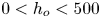 $0< h_o<500$ nm, where
  $h_o$ is the thickness of the oil layer). It is easy to show (Ybert et al. Reference Ybert, Barentin, Cottin-Bizonne, Joseph and Bocquet2007) that the apparent slip length introduced by the said thin lubricant layer is given by (see also the supplementary material available at https://doi.org/10.1017/jfm.2022.162)
 \begin{equation} L_{s,{ow}} = \frac{\mu_{w}}{\mu_{o}}h_o , \end{equation}
where  $\mu _{w/o}$ are the dynamic viscosities of water and oil, respectively. Actual values of the viscosity ratio
  $\gamma _{ow}\equiv \mu _{w}/\mu _{o}$ may be of the order of some units; Scarratt et al. (Reference Scarratt, Zhu and Neto2020) use
  $\gamma _{ow}\approx 4$. According to (1.1), slip due to the oil layer may account for a slip length of up to hundreds of nanometres, depending on the lubricant's nature and thickness.
The second contribution  $L_{s,int}$ to the overall slip length comes from the liquid–liquid interface itself, see figure 1 and is the object of this work. Before discussing its origin, it is important to remark that the two contributions to slip at an LIS simply sum, as can be seen by considering a two-phase Couette flow with a Navier condition at the liquid–liquid interface (more details are presented in the supplementary material):
 \begin{equation} L_{s,{LIS}} = L_{s,ow} + L_{s,int} . \end{equation}
 The slip mechanism ( $L_{s,int}$) at the liquid–liquid interface is much less studied than the one originating from the lower viscosity of the interposed oil layer (
 $L_{s,ow}$) as it is rooted in the molecular interactions at the interface. Recently, the presence of liquid–liquid slip has been invoked to explain unexpected slip measurements at LIS (Scarratt et al. Reference Scarratt, Zhu and Neto2020). Galliero (Reference Galliero2010) studied using molecular dynamics two pure liquids in a shear flow, discussing the dependence of
  $L_{s,int}$ on the miscibility of the two liquids. Results showed that
  $L_{s,int}$ is maximum for poorly miscible liquids, due to the depletion in density occurring at the interface. However, the reported absolute values are of molecular size (
 ${<}1$ nm) and account for an intrinsic slip at liquid–liquid interfaces.
In order to clarify whether  $L_{s,int}$ can be magnified in some conditions and thus give a measurable contribution to the overall slip at LIS, we consider here a liquid–liquid interface with gas dissolved in the liquids – with the understanding that this third species can significantly alter interfacial properties. Dissolved gases are ubiquitous in actual experiments, which are performed in open air (drops at LIS) or in a closed microfluidics environment. Without loss of generality, we characterize the interfacial slip of a well-studied interface, that between two immiscible symmetric liquids, in the presence of an increasing content of gases with different solubilities. We found that interfacial slip can be either of molecular origin (intrinsic slip) or apparent in nature, stemming from the formation of a thin gas layer separating the two liquids. The calculated slip lengths were found to be up to one order of magnitude larger than what is expected for two pure liquids.
The paper is organized as follows. In § 2, the system is introduced and the gas solubilities are characterized – simulations and postprocessing details are given. The reader who is not interested in technical details can jump to § 3, where the results are discussed, including slip lengths as a function of gas content, § 3.1 and the identification of two slip mechanisms: the enrichment of gas of the liquid–liquid interface, § 3.2; and the formation of a gas layer interposed between the two liquids, § 3.3. Section 4 is left for conclusions.
2. Methods
2.1. The system
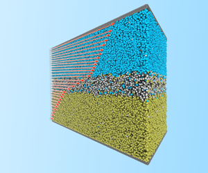
The present work reports the results of non-equilibrium molecular dynamics simulations of a multiphase shear flow (figure 2). The starting point for our investigation is a system composed of two atomic species with symmetric interactions constituting two immiscible liquid phases. Periodic boundary conditions are applied in the directions parallel to the liquid–liquid interface, while rigid atomic walls enclose the system in the third direction. Atoms of a third species were added in increasing amounts to the system in order to investigate their effect on slip properties. Results are reported for different concentrations of this third species and for various interactions strengths with the liquids.

Figure 2. (a) Snapshot of the system: red particles denote liquid 1; pink particles liquid 2; and white particles the third species. The direction orthogonal to the interface plane is the  $z$-axis and the direction going out of the page is the
  $x$-axis. The white arrow represents the shear applied to the upper wall in the
  $y$ direction. (b) Average velocity profile (blue, dotted) along the
  $z$ direction; the interface position is denoted by a dashed line. The velocity jump (
 $\Delta v$) and the slip length (
 $L_s$) are also indicated.
Molecular dynamics simulations were performed using the ‘large-scale atomic/molecular massively parallel simulator’ (LAMMPS) software (Plimpton Reference Plimpton1995). Shearing is obtained by displacing at constant velocity one of the rigid atomic walls that delimit the two liquids, while the remaining wall is constrained to remain still. Thermostatting of the fluid particles is obtained by using a Nosé–Hoover chain thermostat (Martyna, Klein & Tuckerman Reference Martyna, Klein and Tuckerman1992) with  $N_{chain} = 4$ and a dampening parameter of 100 integration time steps, where the time step adopted is
  $\Delta t = 0.003\tau$, with
  $\tau = \sigma (m/\varepsilon )^{1/2}$, where the parameter
  $\sigma$ defines the typical size of the particle and
  $\varepsilon$ the energy scale of the interaction. As customary for simulations of shear flows (Todd & Daivis Reference Todd and Daivis2017), the thermostat acts only on the degrees of freedom that are orthogonal to the shearing direction. Pressure is controlled by applying a constant force on the moving wall in the direction orthogonal to the liquid–liquid interface. This mechanical barostat is a variation on similar schemes in widespread usage (see, e.g. Chinappi & Casciola Reference Chinappi and Casciola2010) and it allows for an accurate control of the hydrostatic pressure. Further simulation details are presented in the supplementary materials. In particular, we checked that the results were consistent with those obtained with different thermostats and that the system was in the linear response regime.
Interatomic interactions between atoms  $i$ and
  $j$ are described by truncated and shifted Lennard–Jones (LJ) potentials
  $U^{LJ}_{ij}$, as follows:
 \begin{equation} U^{LJ}_{ij} = \begin{cases} 4\varepsilon_{\alpha\beta}\left[\left(\dfrac{\sigma_{\alpha\beta}}{r_{ij}} \right)^{12} - \left( \dfrac{\sigma_{\alpha\beta}}{r_{ij}} \right)^{6} \right] + |U_{LJ}(r_{c})| & \text{if} \ r_{ij} \leqslant r_{c} \\ 0 & \text{if}\ r_{ij} > r_{c} { ,} \end{cases} \end{equation}
where indices  $i$ and
  $j$ run over all the atoms and
  $\alpha$ and
  $\beta$ represent the types of atoms
  $i$ and
  $j$, respectively. The total potential energy
  $U$ can be computed by summing
  $U^{LJ}_{ij}$ over all pairs
  $i$,
$i$, $j > i$. A cutoff radius
  $r_{c} = 3.5\sigma$ was used, matching that of Galliero (Reference Galliero2010). Two liquid species were simulated, each defined by LJ parameters
  $\sigma _{11} = \sigma _{22}=\sigma$,
  $\varepsilon _{11}=\varepsilon _{22}=\varepsilon$ and with masses
  $m_{1}=m_{2}=1$. The interactions between the two liquids were modulated by multiplying the energy parameter of the liquid–liquid interactions,
  $\varepsilon _{12}$, by a coefficient
  $k_{liq} = 0.25$, such that
  $\varepsilon _{12} = k_{liq}\varepsilon$; this choice of values is used to render two immiscible liquid phases (Galliero Reference Galliero2010), each occupying one half of the system (figure 2).
A total of 46 398 atoms were used for the entire initial system,  $2812$ of which constitute the two rigid walls and 21 793 for each liquid phase. The system was equilibrated in a box of dimensions
  $L_{x} = 20\sigma$,
  $L_{y} = 40\sigma$ and average height
  $L_{z} = 77.31\sigma$, at the reduced temperature
  $k_B T/\varepsilon = 1$, with
  $k_B$ the Boltzmann constant and
  $T$ the temperature, and keeping the normal pressure, in the
  $z$ direction, constant at
  $P_{z} = 0.4\varepsilon /\sigma ^{3}$, which is held constant also during the shearing of the system. Shearing was obtained by imposing the value
  $|v| = 2.4 \sigma /\tau$, for the streamwise velocity of the upper wall, as illustrated in figure 2.
After an initial equilibration run we introduced different numbers of atoms  $N_{th}$ of a third species. The interactions we considered between the liquids and the third species were symmetric and modulated by multiplying the liquid energy parameter by a constant
  $k_{gas}$, such that
  $\varepsilon _{13} = \varepsilon _{23} = k_{gas}\varepsilon$, while the size parameter was kept constant and equal to unity,
  $\sigma _{13}=\sigma _{23}=\sigma$. Four different values of
  $k_{gas}$ were considered:
  $0.125$,
  $0.25$,
  $0.5$ and
  $1.0$. The factor multiplying the energy parameter,
  $k_{gas}$, made the interactions weaker than or equal to the liquid–liquid ones, thus changing the solubility of the inserted atoms, as characterized below. A broad range of content of the third species was considered, ranging from a minimum of 20 atoms to a maximum of 3600 atoms, corresponding to concentrations going from
  $0.0004\,{\rm wt}\%$ to
  $0.0826\,{\rm wt}\%$, respectively; the weight percentage, having all the atoms the same mass, corresponds to the ratio between the number of the third-species atoms and the number of all the liquid and gas particles in the system.
Atoms of the rigid walls interact only repulsively with atoms of the third species. This is achieved by truncating the interaction potential (LJ parameters:  $\sigma _{3,wall}=2\sigma$,
  ${\varepsilon _{3,wall}=2\varepsilon}$) at its minimum (
 $r_{c} = 2^{1/6}\sigma _{3,wall}$). The purely repulsive interactions of the rigid walls with the third species have been chosen in order to avoid gas atoms accumulating at the liquid–solid interfaces which is not of interest for our study, since the main purpose of the walls is to apply the shear and control the pressure of the system.
Concerning the interactions within the third species, the LJ size parameters were set equal to the liquid ones,  $\sigma _{33}=\sigma$. In order to obtain a gaseous phase, the energy parameter was changed as compared with the value used for liquid species:
  $\varepsilon _{33} = 0.42\varepsilon$. In all cases, the mass of the third species was set to unity,
  $m_{3} = 1$.
2.2. Characterization of the gas solubility in the liquids
In order to characterize solubility of the third species in the two liquids we computed the solvation free energy  $\Delta G_{solv}$ of the third species by thermodynamic integration. We refer to the supplementary material for details about these simulations. This quantity is related to the solubility of the third species via
 \begin{equation} \Delta G_{solv} ={-} k_{B}T \ln(K), \end{equation}
where  $K$ is the dimensionless Henry constant. Results are shown in figure 3; as expected, higher values of
  $k_{gas}$ correspond to lower solvation free energies and thus to higher solubilities of the third species. The results obtained via thermodynamic integration are in good agreement with those calculated from the theory of Reiss et al. (Reference Reiss, Frisch, Helfand and Lebowitz1960) and Wilhelm & Battino (Reference Wilhelm and Battino1971), without fitting – see the supplementary material. The theory is quantitative for intermediate values of
  $k_{gas}$ but is expected to be less accurate for smaller values;
  $k_{gas} = 0$ is not considered in the theory.

Figure 3. Solvation free energy as a function of the parameter  $k_{gas}$ which modulates the interaction between liquid atoms and the dissolved species. Thermodynamic integration results are shown with blue symbols together with a linear fit (blue line), whereas the theory of Reiss et al. (Reference Reiss, Frisch, Helfand and Lebowitz1960) is reported in green. For comparison, we also report, in the relevant
  $k_BT$ units, experimental values of
  $\Delta G_{solv}$ for a selection of gases at 298.15 K; for more information about the experimental data see Sander (Reference Sander2015).
2.3. Data analysis
Velocity and density fields were obtained by dividing the fluid slab into 200 bins along the  $z$-axis and computing averages associated with the corresponding regions of space. The slip length
  $L_s$ was calculated for the liquid–liquid interface at the centre of the computational domain as
 \begin{equation} L_s = \frac{\Delta v}{\dfrac{\partial v}{\partial z}} \end{equation}
where the velocity jump  $\Delta v$ was computed by fitting the linear velocity fields in the two liquid bulks and subtracting the related velocities calculated at the interface; the shear rate
  $\partial v/\partial z$ was calculated as the mean of the shear rates in the two bulk regions (figure 2). The location of the interface
  $z_{int}$ was identified as the coordinate where the two partial density profiles of the liquids cross. This definition of the slip length
  $L_{s}$ is equivalent to the one used by Hu et al. (Reference Hu, Zhang and Wang2010) and to the classical definition of slip length for solid–liquid slip, in which the slip length
  $L_{s}$ is the distance where the extrapolated velocity profile of the upper liquid reaches the velocity of the lower liquid (or solid) at the interface coordinate (figure 2b).
The interface properties, i.e. the interface width  $w_{int}$ and the depletion depth
  $\delta$, were computed using the total density profiles (figure 4). Here
  $w_{int}$ is defined as the distance between the point at which the total density falls below the arithmetic average of the minimum density reached in the depletion region and the bulk value on the liquid
  $1$ side and the point in which the total density raises above the average on the liquid
  $2$ side. The depletion depth,
  $\delta$, is instead quantified as the difference between the total bulk density and the minimum total density in the interface region.

Figure 4. Average density profiles for the two liquid species (green and red lines), for the third species (orange line) and for the total density profiles obtained summing the three profiles (blue line and circles). The definitions of the interface position  $z_{int}$ and the density minimum in the interface region
  $\rho _{min}$, used to calculate depletion depth
  $\delta$, are reported. The black line represents the arithmetic average between the bulk density and the minimum density; the intercepts of this line with the total density profile defines the interface width
  $w_{int}$ (black segment). The cyan dashed line corresponds to the minimum density
  $\rho _{min}$ reached in the depletion zone of the total density profile. The grey dashed line identifies the z coordinate of the interface
  $z_{int}$ defined as the point where the two liquids density profiles intersect. The velocity profile (brown squares) is given in (b) to show the correspondence between the region
  $w_{int}$ and the region where the velocity profile deviates from the linear behaviour of the bulk regions.
3. Results and discussion
3.1. Slip in the presence of gas
We start our presentation of the results discussing the main quantity characterizing slip at liquid–liquid interfaces, i.e. the slip length  $L_s$. Before a third species is added, the slip length is of molecular extent, in agreement with previous reports (Padilla et al. Reference Padilla, Toxvaerd and Stecki1995; Buhn et al. Reference Buhn, Bopp and Hampe2004; Galliero Reference Galliero2010),
  $L_s=6\sigma$, which corresponds to around 2 nm when using the typical characteristic length of water,
  $\sigma =0.31$ nm (Abascal & Vega Reference Abascal and Vega2005). In figure 5, we analyse the effect of atoms of a third species on slip; the slip length is seen to substantially increase or to decrease depending on the strength of the interactions of the liquid with the third phase. Elucidating this process, along with a discussion on the implications of such behaviour for real world microfluidic flows, is the main focus of the present work.

Figure 5. (a) Slip length as a function of the number  $N_{th}$ of third species atoms for the four values of
  $k_{gas}$:
  $0.125$ (blue);
  $0.25$ (green);
  $0.5$ (red);
  $1.0$ (orange). The dashed line represents the value of the slip length without third species, while the dotted vertical line is placed in the region where the transition from dissolved gas to a full gas layer takes place for
  $k_{gas}=0.125$ and
  $0.25$. (b) Snapshots of systems with
  $k_{gas} = 0.125$ at different gas concentrations in the vicinity of the interface.
Figure 5(a) shows that the more soluble gases,  $k_{gas} = 0.5$ and
  $k_{gas} = 1.0$, have a minor effect on the slip properties of the system, causing small changes (
 $k_{gas} = 0.5$) or even a decrease of
  $L_s$ up to
  $50\,\%$ of the starting slip length (
 $k_{gas} = 1.0$). Typical velocity fields and density profiles of these systems are shown in figures 2 and 4. The main effect on slip seems to be due to the density depletion observed at the liquid–liquid interface ensuing from the poor miscibility of the two liquids. In these two cases, the third species accumulates at the interface (and in the bulk, see figure 6) without significantly altering its structure. Over the broad range of concentrations explored, only slight changes in the distribution of the third species were observed. This regime thus consists of a gas-enriched liquid–liquid interface, whose properties are analysed in detail in § 3.2.

Figure 6. Plot of the gas concentration in the bulk region of liquid 1 for the four values of  $k_{gas}$:
  $0.125$ (blue);
  $0.25$ (green);
  $0.5$ (red);
  $1.0$ (orange) measured as number of gas atoms per unit volume versus the number
  $N_{th}$ of third species atoms.
In the less soluble cases ( $k_{gas}=0.125$ and
  $0.25$), as the number of third species atoms
  $N_{th}$ increases, the slip length increases as well (figure 5a). However, for these two cases, the extent of changes is much larger than for the more soluble gases and more complex slip mechanisms emerge. Figure 5(a) clearly shows two different regimes for the slip length: one at low concentrations, below
  $N_{th} \approx 1200$, where the increase in the slip length are moderate and the velocity and density profiles resemble the ones of systems
  $k_{gas} = 0.5$ and
  $k_{gas} = 1.0$ (figures 2 and 4); the other regime starts above
  $N_{th} \approx 1200$ and is characterized by more consistent changes in the slip length, following a linear trend in
  $N_{th}$ with similar slopes for both cases. The density and velocity profiles are significantly different than in the other cases (figure 8) and show the formation of an independent gas layer interposed between the two liquids (see also figure 5b). In this regime, slip is dictated by the (low) viscosity of the gas layer; this mechanism is analysed in detail in § 3.3.
3.2. Intrinsic slip: gas-enriched interface
A first regime can be observed for  $k_{gas} = 0.5$ and
  $k_{gas} = 1.0$ at all gas concentrations, and for
  $k_{gas} = 0.125$ and
  $k_{gas} = 0.25$ when
  $N_{th}$ is below a threshold, which, for the current system is
  $N_{th} \approx 1200$. In this first regime, the gas is observed to progressively accumulate mainly at the liquid–liquid interface filling the depletion region (figure 4). Importantly, the third species shows no particular structure.
The typical velocity profile under shear for these systems is shown in figure 2. The observed behaviour is qualitatively similar to the velocity fields reported by Padilla et al. (Reference Padilla, Toxvaerd and Stecki1995), Galliero (Reference Galliero2010) and Poesio, Damone & Matar (Reference Poesio, Damone and Matar2017) for systems without gas. Two linear regions can be observed in the profiles of streamwise velocity, corresponding to the liquid bulks. An abrupt change in the slope is seen at the liquid–liquid interface, which confirms the presence of some degree of slip between the two liquids. Slip can be quantified in terms of the slip length  $L_s$ with the usual construction in figure 2. This slip is an ‘intrinsic’ one, since it is related to molecular interactions occurring across the liquid–liquid interface. Importantly, the measurable effect of the third phase is an indirect one, in that it modifies the interface width
  $w_{int}$ and its depletion
  $\delta$, see below.
The physical properties  $w_{int}$ and
  $\delta$ characterizing the interface are reported in figure 7 for the gas-enriched interfaces. The plots clearly show that the gas-enrichment of the interface has different effects on its properties depending on the gas–liquid interactions; in turn, these changes are reflected in different trends of the slip length versus
  $N_{th}$.

Figure 7. Interfacial width  $w_{int}$ (a) and depletion depth
  $\delta$ (b) plotted against the number
  $N_{th}$ of third species atoms for the four values of
  $k_{gas}$:
  $0.125$ (blue);
  $0.25$ (green);
  $0.5$ (red);
  $1.0$ (orange). Error bars are comparable to the point size. Dashed lines represent the values of
  $w_{int}$ and
  $\delta$ for the system without third species, dotted vertical line are placed where the transition from dissolved gas to a full gas layer takes place for
  $k_{gas}$
  $0.125$ and
  $0.25$.
It is important to remark that, for  $k_{gas} = 1.0$ and
  $0.5$ the third species can accumulate both in the bulk and at the interface, see figure 6. The local concentration is typically higher at the interface where the density depletion leaves room for the gas; only in the more soluble case
  $k_{gas} = 1.0$ the concentration of gas dissolved in the liquid bulks is comparable to the concentration in the interface region. However, the competition with the bulk is such that the interface is quickly saturated for these cases, which is reflected in marginal changes of the interface properties.
For  $k_{gas} = 1.0$, the interface, i.e. the depletion region, tends to slightly shrink and be replenished, i.e.
  $w_{int}$ and
  $\delta$ decrease as more atoms of the third species are inserted into the system. This corresponds to a decrease of
  $L_{s}$ with
  $N_{th}$, due to an improved momentum transfer at the interface: the gas (marginally) improves the coupling between the two liquids.
For  $k_{gas} = 0.5$, where no substantial changes in the slip length are observed,
  $w_{int}$ and
  $\delta$ correspondingly show no considerable changes. On the other hand, in the case of poorly soluble gases (
 $k_{gas} = 0.125$ and
  $k_{gas} = 0.25$), the depletion region properties show opposite trends as compared with the case
  $k_{gas} = 1.0$, getting (marginally) wider and more depleted as more gas is inserted. The combination of these two effects decreases the momentum transfer at the interfaces and is reflected in significant increases of the slip length, which can reach up to around
  $20\sigma$. In summary, in the intrinsic slip regime we observe a dependence of
  $L_{s}$ on the depletion of the interface region, as quantified by
  $w_{int}$ and
  $\delta$. We remark that depletion is a static, structural property which depends on the microscopic interactions between species and is independent of the velocity, see § 5 of the supplementary material. An increase in
  $\delta$ and
  $w_{int}$, i.e. a thicker and emptier depletion region, causes an increase in the slip length
  $L_{s}$, on the contrary, when the depletion region shrinks and replenishes,
  $L_{s}$ decreases.
3.3. Apparent slip: interposed gas layer
A distinct regime was observed for low solubilities ( $k_{gas} = 0.125$ and
  $k_{gas} = 0.25$) at relatively high concentrations of the third species (
 $N_{th} > 1200$). In this regime, we observed the formation of an independent layer rich in the third species taking the place of the original liquid–liquid interface, see figure 8. The density of this layer is lower than that of the liquids and its structure is that of a gas. In particular, independent equilibrium simulations at identical temperature, pressure and compositions (see the supplementary material, figure S11) show that the density and the radial distribution functions correspond to those of a bulk gas, allowing us to confirm that the interposed layer consists indeed of a bulk-like ‘gas phase’.

Figure 8. Density (a) and velocity profiles (b) in the region close to the interfaces for  $k_{gas} = 0.125$ and
  $N_{th}=3600$. The profiles show the formation of a third phase between the two liquids characterized by a lower density as compared with the two liquid phases. The velocity profile does not exhibit anymore an abrupt change but three approximately linear regions.
The density profiles in the gas-layer regime (figure 8a) reveal significant differences as compared with the enriched interface case. The original liquid–liquid interface gets gradually substituted by a well-defined slab of a new lower-density phase mainly constituted by third species atoms and saturated with the two original liquids in solution. With the increase in  $N_{th}$ in the system, the thickness of the gas layer increases, as shown by the linear growth of
  $w_{int}$, while the concentration of gas dissolved in the original liquid phases remains constant at saturation levels (figure 6). On the other hand, the depletion
  $\delta$ remains constant since the density minimum is reached in correspondence of the new phase, which settles at its bulk value.
The velocity profiles in figure 8(b) show that the velocity gradient increases in the interposed layer, due to the lower viscosity of the gas as compared with that of the liquids. The net effect of progressively substituting the liquid–liquid interface by a discrete slab of gas phase is thus that of deteriorating momentum transfer between the two liquids. In this scenario, it is possible to compute an apparent slip length, which accounts for the decreased friction at the interface in an effective way. Such a concept is valid at intermediate scales at which the thickness of the gas layer can be neglected.
Already in the presence of a gaseous layer with a thickness of few atomic diameters we observed large effective slip between the two liquids. Slip increases as additional gas is added and enriches the layer. This very large slip is not to be confused with intrinsic slip at the liquid–liquid interface, since, as the velocity profile shows, there is no abrupt change in the velocity field, but an apparent slip mediated by the low viscosity gaseous layer interposed between the two liquids, see figure 8.
Figure 9(a) shows that the slip length in the gas-layer regime increases linearly with the width of the gaseous slab and thus with  $N_{th}$. Furthermore, it can be noticed how the proportionality between
  $L_{s}$ and
  $N_{th}$ is the same for various values of the gas–liquid interactions, as shown by the two curves for
  $k_{gas} = 0.125$ and
  $k_{gas} = 0.25$ having the same slope. This finding further confirms that the interposed layer indeed reaches bulk properties which depend almost solely on the gas properties and not on its interactions with the liquid. The only dependence on
  $k_{gas}$ is indirect and concerns the creation of the layer, which only occurs for gases whose solubility is sufficiently low to allow the gas concentration in the liquid bulk to quickly reach saturation.

Figure 9. (a) Data for  $k_{gas} = 0.125$ (blue circles) and
  $k_{gas} = 0.25$ (green squares) of the apparent slip length as function of the interface width
  $w_{int}$ for the systems where the gas layer is fully formed. The blue and green lines are a linear fit to the data, giving as result a theoretical value of the viscosity ratio
  $\gamma = 4.84$ for
  $k_{gas} = 0.125$, and
  $\gamma = 4.74$ for
  $k_{gas} = 0.25$. The red dotted line has slope
  $\gamma =4.87$, calculated using the viscosities obtained via Green–Kubo formalism. (b) Sketch of the three-fluids model used to find analytically a relation between the interposed layer thickness and the slip length. The velocity jump is defined in analogy with the one represented in figure 2.
Employing the framework introduced in § 1.1, we compute the apparent slip length  $L_{s}$ introduced by an intervening gas layer of given viscosity. At variance with figure 1, we solve for a triphase Couette flow in which the two liquids are symmetric and a gas layer is interposed between them, see figure 9(b). We refer the reader to the supplementary material for the full derivation. The main result is that
  $L_{s}=(\gamma - 1)\,w$, with
  $\gamma = \mu _{l}/\mu _{g}$ and
  $w$ the thickness of the gas layer.
The red dashed line in figure 9(a) shows a quantitative accord of the slope predicted by the macroscopic Couette model with the numerical simulations. Importantly, we found that the ratio of liquid and gas phase viscosity as deduced from a linear fit of the measured velocity profiles is consistent with independent estimates of  $\gamma$ via the viscosities of the various phases obtained in equilibrium simulations via the Green–Kubo formalism (see the supplementary material for more information).
We further note that, in the gas-layer regime, two independent gas–liquid interfaces form. For both of them the velocity profile is smooth (figure 8b) and does not show the distinctive jump of the liquid–liquid interface, cf. figure 2(b). In other terms, the slip connected to gas–liquid interfaces is vanishingly small, which likely originates in the capacity of a dense, unstructured, and partially soluble fluid – a gas – to adhere to a liquid interface: the total density profile indeed shows a smooth change between the liquid and gas bulk values (figure 8a) without the depletion characterizing the interface between two poorly miscible structured fluids (figure 4). Therefore, one cannot introduce additional slip lengths connected to the two gas–liquid interfaces. We remark that this result is obtained in a rather different regime than previous studies on rarefied gases at solid surfaces (de Gennes Reference de Gennes2002; Ramisetti et al. Reference Ramisetti, Borg, Lockerby and Reese2017). Nonetheless, the vertical offset between the two straight lines at  $k_{gas} = 0.125$ and
  $k_{gas} = 0.25$ in figure 9 seems to suggest a minor role of the gas–liquid interactions on the overall slip length.
3.4. Intrinsic and apparent slip at LISs
At LISs, the total slip length is given by the sum of the slip due to the lubricant layer  $L_{s,ow}$ and that of the liquid–liquid interface
  $L_{s,int}$, see (1.2). The present result shows that
  $L_{s,int}$ can have two different origins: intrinsic, when it emerges from the structure of the liquid–liquid interface, in this case, enriched by a gas phase; or apparent, when a discrete gas layer forms between the two liquids. Only in the case of the gas layer, the contribution of
  $L_{s,int}$ to (1.2) is significant, up to tens of nanometres. Such values may at least partially explain the large slip lengths reported in recent experiments (Scarratt et al. Reference Scarratt, Zhu and Neto2020). In the light of the present results, further experiments controlling the gas content are needed in order to assess the relevance of such mechanism in conditions of technological relevance.
Interestingly, we do not observe any breakdown mechanism of the gas layer even at the highest considered gas content, nor its stability is influenced by the shear or the pressure, see the supplementary material. In addition, density profiles like that in figure 8(a) show that the gas layer has reached bulk-like characteristics. Together, these two considerations suggest that, under some circumstances, thick gas layers may form at LIS accounting for very large slip. In particular, it is required that the gas has poor solubility and no means to escape in the environment, such that it is forced to accumulate at the liquid–liquid interface. This might be the case for closed systems, such as microfluidic chips, where gas-induced slip lengths of tens of nanometres, such as those computed here, may be important both for interpreting available experiments and to decrease friction at LIS.
One is further tempted to speculate that gas layers similar to those reported here may also form at liquid–solid interfaces, potentially leading to significant slip (de Gennes Reference de Gennes2002). Gas accumulation is indeed known to occur for hydrophobic substrates (Tortora et al. Reference Tortora, Meloni, Tan, Giacomello, Ohl and Casciola2020), leading to the formation of surface nanobubbles (Lohse & Zhang Reference Lohse and Zhang2015); however, further investigation is needed in order to assess the role of the nanobubble shape and pinning on slip. Indeed, it has been reported that protruding nanobubbles may actually decrease slip or even increase friction (Maali & Bhushan Reference Maali and Bhushan2013).
4. Conclusions
Non-equilibrium molecular dynamics simulations have been instrumental to provide microscopic insights into slip at liquid–liquid interfaces in the presence of a third species. Dissolved gases are ubiquitous in real world and experimental applications, and are found to significantly alter the microscopic structure of interfaces, resulting in macroscopically observable effects on the flow. More fundamentally, a rich phenomenology is reported for enriched liquid–liquid interfaces, which should be taken into account when considering the boundary condition between two liquids in microscale and nanoscale flows.
In this work, the effect of dissolving a third species on the slip properties was found to depend on the solubility of the enriching species and on the gas content of the system. At low concentrations, the third species tends to accumulate at the liquid–liquid interface altering the local density, thus regulating its intrinsic slip length: poorly soluble species tend to deplete it, thereby effectively reducing the viscous coupling between the two liquids. On the other hand, addition of soluble species replenishes the liquid–liquid interface, increasing the viscous coupling between the liquids.
As the total content of the third species is increased above a critical value, the less soluble species quickly reach saturation in the liquid bulks, leading to the formation of an independent, low-density gas layer interposed between the two liquids. This second regime is associated with large apparent slip lengths scaling linearly with the thickness of the gaseous slab and with the liquid-to-gas viscosity ratio as quantitatively explained by a three-fluids model. A thickness of the gas layer just above  $10$ molecular radii (
 ${\sim }3$ nm for water) was observed to yield apparent slips exceeding the original liquid–liquid values by roughly one order of magnitude.
The present results reveal a rich phenomenology of relevance for all liquid–liquid interfaces. Of particular interest are LIS for which large slip lengths have been reported (Solomon et al. Reference Solomon, Khalil and Varanasi2014; Scarratt et al. Reference Scarratt, Zhu and Neto2020), but whose origin is largely unknown. Present simulations suggest that, whereas the intrinsic liquid–liquid slip, even at enriched interfaces, is always very small and comparable to the liquid particle size, the potential build-up of discrete gas layers of nanometre width may contribute to the giant slip lengths measured at LIS. Further studies are needed to verify the presence of such a gas layer in actual experimental conditions and the means to control its thickness. This knowledge will provide an effective and robust means to achieve large slip at LIS to be used, e.g. in drag reduction applications.
Supplementary material
Supplementary material is available at https://doi.org/10.1017/jfm.2022.162.
Acknowledgements
We gratefully acknowledge thoughtful discussion with M. Chinappi, S. Meloni and C. Neto.
Funding
This research is part of a project that has received funding from the European Research Council (ERC) under the European Union's Horizon 2020 research and innovation programme (grant agreement no. 803213). This work has been supported by the project ‘Understanding and tuning friction through nanostructure manipulation’ (UTFROM) funded by MIUR Progetti di Ricerca di Rilevante Interesse Nazionale (PRIN) Bando 2017 – grant 20178PZCB5. The authors acknowledge PRACE for awarding us access to Marconi100 at CINECA, Italy.
Declaration of interests
The authors declare no conflict of interest.
Data availability statement
Raw data are available at https://doi.org/10.5281/zenodo.6327516.
Author contributions
A.G. and A.T. designed research. E.T. performed the simulation; A.G., A.T., and E.T. analysed data and wrote the manuscript.


 Open access