


1. Introduction
Thermoacoustic instabilities result from the constructive coupling between flames and acoustics. They frequently occur in rocket and aircraft engines, as well as in gas turbines for power generation. They are unwanted because the vibrations they induce lead to mechanical fatigue and sometimes even to destruction of the combustors. Understanding, modelling and controlling this phenomenon is the goal of many research programs. An important part of this research is focused on the specific case of annular combustion chambers, which are generally used in aeronautic engines for their light weight and their compactness. In these chambers, the thermoacoustic instabilities frequently involve eigenmodes exhibiting an azimuthally modulated sound pressure distribution, where the combustion chamber circumference is a multiple of the acoustic wavelength (e.g. Berger et al. Reference Berger, Hummel, Schuermans and Sattelmayer2018; Mazur et al. Reference Mazur, Nygård, Dawson and Worth2019; Kim et al. Reference Kim, Gillman, Emerson, Wu, John, Acharya, Isono, Saitoh and Lieuwen2020). Bauerheim, Nicoud & Poinsot (Reference Bauerheim, Nicoud and Poinsot2016) reviewed the recent development of analytical and computational methods for predicting the linear stability and the nonlinear dynamics of these azimuthal modes. With sufficient calibration data and adequate description of the nonlinear response of the flame to acoustic perturbations, thermoacoustic network models reproduce the dynamics of real systems relatively well at very low computational costs (e.g. Schuermans, Paschereit & Monkewitz Reference Schuermans, Paschereit and Monkewitz2006; Morgans & Stow Reference Morgans and Stow2007; Noiray, Bothien & Schuermans Reference Noiray, Bothien and Schuermans2011). Current research efforts also include the development of purely analytical models in idealised geometries (e.g. Faure-Beaulieu & Noiray Reference Faure-Beaulieu and Noiray2020; Li, Morgans & Yang Reference Li, Morgans and Yang2020a; Ghirardo & Gant Reference Ghirardo and Gant2021), efficient numerical methods to account for complex boundary conditions in truncated geometries (e.g. Fournier et al. Reference Fournier, Haeringer, Silva and Polifke2021; Laurent, Badhe & Nicoud Reference Laurent, Badhe and Nicoud2021), or adjoint-based methods for the optimisation of the combustor geometry with regard to the linear stability of the azimuthal modes (Mensah et al. Reference Mensah, Magri, Orchini and Moeck2019; Yang et al. Reference Yang, Sogaro, Morgans and Schmid2019).
In general, the instantaneous state of these so-called azimuthal modes belongs to one of the following three categories: (i) standing mode, when the angle defining the position of the nodal lines remains constant or varies very slowly with respect to the acoustic period, (ii) spinning mode, when the mode shape nodes travel in the clockwise (CW) or counterclockwise (CCW) direction along the chamber circumference at the speed of sound, or (iii) mixed mode, which is a linear combination of the two previous types of state. There are also situations where this classification is not sufficient. For example, Bourgouin et al. (Reference Bourgouin, Durox, Moeck, Schuller and Candel2015) discovered a peculiar type of thermoacoustic dynamics for which the sound pressure level has only one minimum along the combustor circumference, which they called the slanted mode and which was afterwards further investigated by Prieur et al. (Reference Prieur, Durox, Schuller and Candel2017) and modelled by Moeck et al. (Reference Moeck, Durox, Schuller and Candel2018) as the synchronisation between a pure longitudinal mode and an azimuthal mode with very close eigenfrequencies.
In the present work, we focus on a particular steady state which can be described as a beating mode and was reported by Indlekofer et al. (Reference Indlekofer, Faure-Beaulieu, Noiray and Dawson2021b): the self-oscillating azimuthal mode periodically alternates between CW and CCW spinning directions. The regularity of this phenomenon suggests that the alternation of the spinning direction is not caused by turbulence-induced stochastic perturbations of the limit cycle, as was shown to be the case in some recent studies (e.g. Noiray & Schuermans Reference Noiray and Schuermans2013; Hummel et al. Reference Hummel, Berger, Stadlmair, Schuermans and Sattelmayer2018; Mazur et al. Reference Mazur, Nygård, Dawson and Worth2019; Faure-Beaulieu et al. Reference Faure-Beaulieu, Indlekofer, Dawson and Noiray2020), but by an underlying deterministic mechanism, which we aim to explain in the present work. We will achieve this goal with a model that includes small, but not negligible, resistive and reactive asymmetries. The former are associated with a non-uniform azimuthal distribution of the resistive part of the flames and of the flow transfer functions, and the latter with a non-uniform distribution of the reactive part of these transfer functions, with inhomogeneities of the temperature field, or with geometrical deviations from perfect axisymmetry. So far, the impact of asymmetries on azimuthal modes has focused on resistive asymmetries. This is probably due to the fact that, unlike reactive asymmetries, resistive asymmetries govern the linear stability of the modes (e.g. Noiray et al. Reference Noiray, Bothien and Schuermans2011). We will show here that reactive asymmetries, on the other hand, have a major effect on the nonlinear dynamics and are the fundamental cause of the beating mode. Moreover, we will demonstrate an unintuitive result: the fact that they induce reflectional symmetry breaking and thus favour a spinning direction, which until now was attributed exclusively to the presence of an azimuthal flow.
2. Experimental observations
Experiments were performed with an annular combustor operated at atmospheric condition, sketched in figure 1. The fuel was a 70 %  $\textrm {H}_2$ and 30 % $\textrm {CH}_4$ blend by thermal power. It was mixed with air upstream of the plenum. The mixture flowed through twelve burners that uniformly distributed around the annular chamber, which was made of two concentric water-cooled cylindrical walls of 127 and 212 mm diameter. The combustor thermal power was fixed to 48 kW (4 kW per burner) and the equivalence ratio was varied between $\varPhi =0.4$ and $\varPhi =0.65$, corresponding to near blow-off and flashback conditions. More details about the set-up can be found in Mazur et al. (Reference Mazur, Nygård, Dawson and Worth2019).
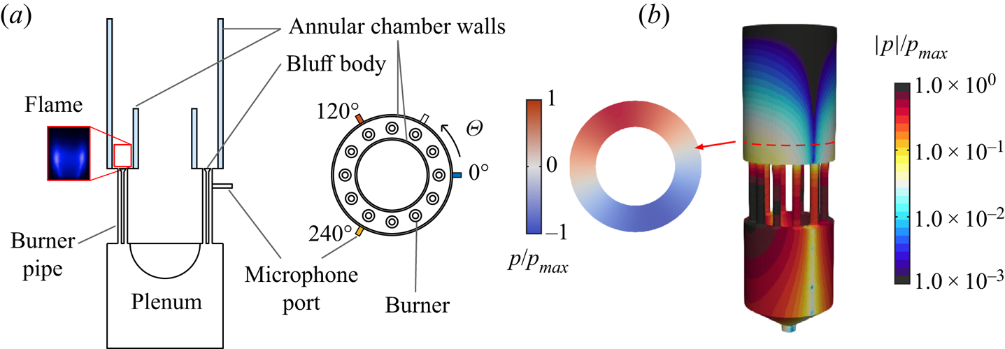
Figure 1. (a) Sketches of the side and top views of the experimental annular combustor. (b) Acoustic eigenmode involved in the thermoacoustic instability, obtained by solving the Helmholtz equation with approximated temperature field and boundary conditions.
Four Kulite XCS-093-05D microphones were used for acoustic pressure measurements; they were mounted to the burner inlet pipes at azimuthal positions  $0^{\circ }$, $60^{\circ }$, $120^{\circ }$ and $240^{\circ }$. Above $\varPhi =0.5$, the system is thermoacoustically unstable, with self-sustained oscillations around 900 Hz. The operating condition $\varPhi =0.575$ is used in this work to illustrate the significant effect of tiny resistive and reactive asymmetries of the combustor upon the stationary thermoacoustic dynamics. The transient thermoacoustic dynamics observed during linear sweeps of the air mass flow, for which $\varPhi$ was increased from 0.5 to 0.6 in 20 s, was investigated by Indlekofer et al. (Reference Indlekofer, Faure-Beaulieu, Noiray and Dawson2021b).
Figure 2 shows the acoustic pressure time traces and power spectral densities (PSDs) in three of the burner pipes at the stationary condition  $\varPhi =0.575$. The time traces in figure 2(a) exhibit a distinctive amplitude beating. Four coloured dotted lines indicate four successive phases of the beating cycle, which are shown in figure 2(b). During the first phase, the three microphones show sinusoidal oscillations of similar amplitudes and with phase shifts of $120^{\circ }$ between them: the azimuthal thermoacoustic eigenmode spins around the chamber at the speed of sound. The order of the time traces indicates a CW spinning direction. In the second phase, all the signals oscillate in phase or in phase opposition, but with different amplitudes: the azimuthal thermoacoustic eigenmode is standing. The amplitude at the azimuth $240^{\circ }$ is small, indicating that the nodal line is close to that angle. During the third phase, the eigenmode spins again, but the order of the time traces is inverted: the wave propagates in the CCW direction. In the fourth phase, the mode is again standing, but its nodal line orientation is different from that of the second phase. This cyclic inversion of the spinning direction is very stable at this operating condition. We note that the raw signals are almost perfectly sinusoidal, with a dominant peak in the PSD that is four orders of magnitude larger than the background spectral content. The time trace of the microphone placed at $\varTheta =60^{\circ }$ (not shown in figure 2) is the opposite of the one measured at $\varTheta =240^{\circ }$, which corresponds to an odd azimuthal order, and the amplitudes at the three equispaced positions are different, so the order is not a multiple of three. Helmholtz solver computations using an approximated temperature distribution were performed (Indlekofer et al. Reference Indlekofer, Faure-Beaulieu, Noiray and Dawson2021b) and predict the existence of a first-order azimuthal acoustic mode at 900 Hz, matching well with the measured peak frequency of the thermoacoustic mode at 894 Hz in the experiment. A closer view of the PSD in figure 2(d) shows that there are in fact two peaks separated by about 2 Hz, which corresponds to the frequency of the beating. This suggests that the beating originates from explicit symmetry-breaking between a pair of approximately coincident eigenmodes that would be degenerate in an ideal rotationally symmetric configuration (Noiray et al. Reference Noiray, Bothien and Schuermans2011).

Figure 2. (a) Acoustic time traces from three equispaced microphones for  $\varPhi =0.575$; the first two traces in the shaded area are shown on the right. (b) Short intervals illustrating the four phases of a beating cycle with the colour code corresponding to (a). From left to right: mixed CW spinning, standing, mixed CCW spinning, standing. Panels (c)–(d) show the PSD over a broad and a narrow frequency range around the dominant peak.
The quaternion-based anzatz for azimuthal waves introduced by Ghirardo & Bothien (Reference Ghirardo and Bothien2018) is now used for decomposing the acoustic pressure field. Its real part is
 \begin{equation} p(\varTheta,t)=A\cos(\varTheta-\theta)\cos(\chi)\cos(\varOmega t + \varphi)+A\sin(\varTheta-\theta)\sin(\chi)\sin(\varOmega t + \varphi), \end{equation}
where  $\varOmega$ is the acoustic pulsation, $\varTheta$ is the azimuthal coordinate, and $A$,
$A$,  $\theta$, $\chi$ and $\varphi$ are state variables, which vary slowly in comparison to the acoustic period $2{\rm \pi} /\varOmega$, and which describe the instantaneous state of the thermoacoustic eigenmode. The variable $A$ describes the amplitude of the mode, $\theta$ is the orientation of its standing wave component, $\varphi$ is its temporal phase drift, and $\chi$ indicates its nature: it is a pure standing mode when $\chi =0$, a pure CW (respectively CCW) spinning mode when $\chi =-{\rm \pi} /4$ (respectively ${\rm \pi} /4$) or a mixed mode when $0<|\chi |<{\rm \pi} /4$. The extraction of these slow variables from the filtered microphone time traces is explained by Ghirardo & Bothien (Reference Ghirardo and Bothien2018). Their time evolution for $\varPhi =0.575$ is shown in figure 3(a). The first noticeable feature is the low-frequency periodic oscillation of $\chi$ between $-{\rm \pi} /4$ and ${\rm \pi} /4$, which means that the mode alternates between CW and CCW spinning states. Furthermore, $\theta$ also oscillates, with rapid changes between ${\rm \pi} /4$ and $3{\rm \pi} /4$. The evolution of $\varphi$ presents stair steps that are synchronised with the fluctuations of the other variables. The amplitude $A$ fluctuates, but in contrast with $\chi$, $\theta$ and
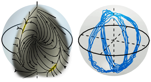
  $\varphi$ the oscillations are relatively small compared to the mean amplitude. As proposed by Ghirardo & Bothien (Reference Ghirardo and Bothien2018), a convenient way to represent the evolution of the eigenmode state is the Bloch sphere: a spherical coordinate system is used, where $A$ is the radius, $2\chi$ is the elevation angle (the equator corresponds to standing modes, the poles to purely spinning modes) and $\theta$ is the azimuth. Figures 3(e) and 3(d) show a portion of the experimental trajectory describing the eigenmode state and its probability density function (p.d.f.) in this coordinate system, revealing regular closed orbits. It is worth mentioning that this intriguing beating is not observed when the thermal power of the combustor is increased by 50 % (72 kW) with equivalence ratio fixed between $\varPhi =0.5$ and $\varPhi =0.6$ (Faure-Beaulieu et al. Reference Faure-Beaulieu, Indlekofer, Dawson and Noiray2020; Indlekofer et al. Reference Indlekofer, Faure-Beaulieu, Dawson and Noiray2021a), which will be discussed in the results section.

Figure 3. Dynamics of the state variables: (a) extracted from the experiment; (b) simulated with (3.6) without noise, i.e.  $\varGamma =0$ (solid lines), and extracted from a simulation of the wave equation (3.5) (dashed lines); (c) simulated with (3.6) with stochastic forcing; (d) p.d.f. from 100 s of experimental data in the Bloch sphere representation; (e) portion of the experimental state trajectory. Panels (f)–(g) are simulated trajectories of panels (b)–(c). Simulation parameters: $\varOmega =2{\rm \pi} \times 894$ Hz, $\alpha =100\ \textrm {s}^{-1}$, $\beta =160\ \textrm {s}^{-1}$, $\kappa =2.5\times 10^{-4} \ \textrm {Pa}^{-2}\ \textrm {s}^{-1}$, $\varGamma =10^{12}\ \textrm {Pa}^{2}\ \textrm {s}^{-3}$, $a_2=m_2= 6\times 10^{-2}$, $\varTheta _{\mu 2}=0$, $\varTheta _{\alpha 2}=4{\rm \pi} /5$.
3. Model
We now propose a low-order model which reproduces the beating phenomenon by explicitly introducing asymmetries in the system. The starting point is the three-dimensional wave equation for the acoustic pressure  $p$, in the presence of unsteady heat release rate $\dot {Q}$, without mean flow or temperature gradients:
 \begin{equation} \frac{\partial^{2} p}{\partial t^{2}}-c^{2} \nabla^{2}p = (\gamma-1)\frac{\partial \dot{Q}}{\partial t}, \end{equation}
where  $c$ is the sound speed and $\gamma$ the adiabatic index. Following Faure-Beaulieu & Noiray (Reference Faure-Beaulieu and Noiray2020), an idealised version of the combustor is considered: an annular waveguide of mean radius $\mathcal {R}$, thickness $\delta _\mathcal {R}\ll \mathcal {R}$ and height $\mathcal {Z}$ described with cylindrical coordinates $(r,\varTheta ,z)$. The operators $\langle g\rangle _\sigma =\sigma ^{-1}\int _{\sigma } g(r,\varTheta ,z,t)\, \mathrm {d}z\, \mathrm {d}r$ and $\langle g\rangle _\upsilon =\upsilon ^{-1}\int _{\upsilon } g(r,\varTheta ,z,t) r\, \mathrm {d}\varTheta \, \mathrm {d}r\, \mathrm {d}z$ will be used to average quantities over the cross-section $\sigma =\delta _{\mathcal {R}}\mathcal {Z}$, and in the volume $\upsilon =\mathcal {R}\delta _\varTheta \sigma$ of a small angular sector of the annular combustor. The volume averaging is thus applied to (3.1). Regarding the first term, when $\delta _\varTheta \rightarrow 0$, one has $\langle \partial ^{2} p/\partial t^{2}\rangle _\upsilon \rightarrow \partial ^{2} \langle p\rangle _\sigma /\partial t^{2}$. The divergence theorem is applied to the second term. The resulting surface integral is split between the poloidal cross sections and the combustor boundary as $\langle \nabla ^{2} p \rangle _\upsilon =T_1+T_2$, where
 \begin{equation} \left.\begin{gathered} T_1= \dfrac{1}{\mathcal{R}\delta_\varTheta}\left\langle\dfrac{\partial p}{{r\partial \varTheta}}\left(r,\varTheta+\frac{\delta_\varTheta}{2},z,t\right)-\dfrac{\partial p}{{r\partial \varTheta}}\left(r,\varTheta-\frac{\delta_\varTheta}{2},z,t\right)\right\rangle_\sigma\\ \quad \text{and}\quad T_2=\dfrac{1}{\upsilon} \int_{\varsigma} \boldsymbol{\nabla} p\boldsymbol{\cdot}\boldsymbol{n}\,\mathrm{d}S, \end{gathered}\right\} \end{equation}
and where  $\boldsymbol {n}$ is the outwards normal vector to the surface element $\mathrm {d}S$ of the lateral surface $\varsigma$ of the volume $\upsilon$, whose area is $2(\mathcal {Z}+\delta _\mathcal {R})\mathcal {R}\delta _\varTheta$. For $\delta _\varTheta \rightarrow 0$, and considering that $\delta _\mathcal {R}\ll \mathcal {R}$, we have $T_1\rightarrow \mathcal {R}^{-2} \partial ^{2} \langle p\rangle _\sigma /\partial \varTheta ^{2}$. The second term $T_2$ accounts for the effect of the combustor boundaries. For the limit case of rigid walls and choked combustor inlet and outlet, the normal acoustic pressure gradient on $\varsigma$ is zero and $T_2$ vanishes. In the present work, a general boundary condition is given by the specific acoustic impedance averaged over $\varsigma$ and defined by $Z(\varTheta ,\omega )=\hat {p}/(\rho c \,\hat {\boldsymbol {u}}\boldsymbol {\cdot } \boldsymbol {n})$, where $\omega$ is the angular frequency, $\rho$ is the density, and $\hat {p}$ and $\hat {\boldsymbol {u}}$ are the Laplace transforms of the acoustic pressure and velocity. By considering the normal component of the momentum balance on $\varsigma$, one can write $\boldsymbol {\nabla } \hat {p}\boldsymbol {\cdot } \boldsymbol {n}= -\text {i}\omega \rho \hat { \boldsymbol {u}}\boldsymbol {\cdot } \boldsymbol {n}= -\text {i}\omega \hat {p}/Zc$. It is now reasonable to assume that at any azimuthal position, $Z$ is almost constant in the narrow frequency range around the thermoacoustic instability peak in the PSD. In the idealised geometry, the angular frequency of the first azimuthal eigenmode peak is $\varOmega =c/\mathcal {R}$. Back in the temporal domain, this gives $c\boldsymbol {\nabla } p\boldsymbol {\cdot } \boldsymbol {n} = -(Y\varOmega p + X\partial p/\partial t)/(X^{2}+Y^{2})$, where $X(\varTheta )=\textrm {Re}(Z)$ and $Y(\varTheta )=\textrm {Im}(Z)$ are the specific resistance and reactance of the annular combustor boundary at angular frequencies around $\varOmega$. Then when $\delta _\varTheta \rightarrow 0$, one has
 \begin{equation} T_2\rightarrow -\dfrac{Y\varOmega}{\delta_\mathcal{R} \mathcal{Z} (X^{2}+Y^{2}) c} \int_{\ell } p\,\text{d}l -\dfrac{X}{\delta_\mathcal{R} \mathcal{Z} (X^{2}+Y^{2}) c}\dfrac{\partial}{\partial t}\left(\int_{\ell } p\,\text{d}l \right), \end{equation}
where  $\ell$ is the boundary of the slice $\sigma$. Assuming that the integral of the acoustic pressure along that boundary is proportional to the average acoustic pressure over the slice (with $K$ the proportionality constant), we have $T_2\rightarrow -(\mu /c^{2})\,\langle p \rangle _\sigma -(\varrho /c^{2}) \partial \langle p\rangle _\sigma /\partial t$, where $\varrho (\varTheta )=XKc/[\delta _\mathcal {R}\mathcal {Z}(X^{2}+Y^{2})]$ is a damping rate that is positive if the boundary is dissipative, and $\mu (\varTheta )=Y\varOmega Kc/[ \delta _\mathcal {R}\mathcal {Z}(X^{2}+Y^{2})]$. Consequently, the wave equation for $\langle p \rangle _\sigma$ is
 \begin{equation} \dfrac{\partial^{2} \langle p \rangle_\sigma}{\partial t^{2}} + \varrho(\varTheta)\dfrac{\partial \langle p \rangle_\sigma}{\partial t} + \mu(\varTheta)\langle p \rangle_\sigma - \varOmega^{2}\dfrac{\partial^{2} \langle p \rangle_\sigma}{\partial \varTheta^{2}} = (\gamma-1)\dfrac{\partial \langle\dot{Q}\rangle_\sigma}{\partial t}. \end{equation}
From now on, we will only consider the one-dimensional azimuthal wave equation (3.4) and drop the brackets  $\langle \cdot \rangle _\sigma$. To model the nonlinear flame response to acoustic perturbations, we use a classic cubic saturation model $(\gamma -1)\dot {Q}=\beta (\varTheta ) p-\kappa p^{3}$, used for instance by Noiray et al. (Reference Noiray, Bothien and Schuermans2011), Moeck et al. (Reference Moeck, Durox, Schuller and Candel2018) and Li et al. (Reference Li, Wang, Wang and Zhao2020b). It should be noted that this simple flame response model can be considered a first approximation of the time-domain counterpart of the flame describing function, which can be measured with dedicated experiments, as recently done by Nygård, Ghirardo & Worth (Reference Nygård, Ghirardo and Worth2021). Also, the inherent time delay between the acoustic oscillations in the burners and the resulting response of the flames does not explicitly appear in the model. Its effect on the thermoacoustic dynamics is implicitly contained in the effective gain $\beta$ and saturation constant $\kappa$. Bonciolini et al. (Reference Bonciolini, Faure-Beaulieu, Bourquard and Noiray2021) showed that such a model does reproduce the delayed thermoacoustic feedback when the delay is short compared to the inverse of the instability growth rate. It is worth mentioning that alternative flame response models exist, such as the one proposed by Ghirardo & Juniper (Reference Ghirardo and Juniper2013), which depend not only on the acoustic pressure load across the burners, but also on the azimuthal acoustic velocity in the chamber, a dependency that has been the subject of several experimental studies (e.g. O'Connor Reference O'Connor2015). However, we do not include such possible additional effects in our model; rather, we keep it as simple as possible, which allows us to fully reproduce the experimental observations. We add a stochastic source term $\varXi$, which accounts for the effect of turbulence on the thermoacoustic system, and which is considered as a white noise. Recalling that $\partial ^{2} p/\partial \varTheta ^{2}=-p$ for the first azimuthal eigenmode, one obtains
 \begin{equation} \dfrac{\partial^{2} p }{\partial t^{2}} + \left(\varrho(\varTheta)-\beta(\varTheta) + 3\kappa p^{2}\right)\dfrac{\partial p }{\partial t} - \left(\varOmega^{2}+\mu(\varTheta)\right)\dfrac{\partial^{2} p }{\partial \varTheta^{2}} = \varXi(\varTheta,t). \end{equation}
The term  $\mu (\varTheta )$ can be interpreted as a spatial modulation of the effective sound speed along the annular chamber. Here, this modulation comes from azimuthal asymmetries of the acoustic impedance on the combustor boundaries, but the same equation can be obtained if one considers asymmetries of the chamber geometry, of the temperature field or of a flame response model with imaginary component. Although the linear gain of the flame response $\beta$ can in general be complex and depend on $\varTheta$, it will be assumed here to be a real constant.
In the present study, an eigenmode with first-order azimuthal component dominates the thermoacoustic dynamics. The first harmonic is four orders of magnitude lower than the main peak in the PSD shown in figure 2, which justifies the use of the ansatz (2.1) in the wave equation (3.5). The spatio-temporal averaging, which has been proposed by Faure-Beaulieu & Noiray (Reference Faure-Beaulieu and Noiray2020), is applied to the latter equation. This leads to the following system of Langevin equations for the slow variables  $A$,
$A$,  $\chi$, $\theta$ and $\varphi$:
 \begin{equation} \left.\begin{gathered}\dot{A}=\dfrac{\beta-\alpha}{2}A-\dfrac{a_2 \alpha }{4}\cos(2[\theta-\varTheta_{\alpha 2}])\cos(2\chi)A -\dfrac{3\kappa}{64}[5+\cos(4\chi)]A^{3}+\dfrac{3\varGamma}{4\varOmega^{2} A}+\zeta_A,\\ \dot{\chi}=\dfrac{3\kappa}{64}\sin(4\chi)A^{2}+\dfrac{a_2 \alpha }{4}\cos(2[\theta-\varTheta_{\alpha 2}])\sin(2\chi)+\dfrac{m_2\varOmega}{4}\sin(2[\theta-\varTheta_{\mu 2}])\\ -\dfrac{\varGamma\tan(2\chi)}{2\varOmega^{2} A^{2}}+\dfrac{\zeta_\chi}{A},\\ \dot{\theta}=\dfrac{a_2 \alpha }{4}\dfrac{\sin(2[\theta-\varTheta_{\alpha 2}])}{\cos(2\chi)}-\dfrac{m_2\varOmega}{4}\cos(2[\theta-\varTheta_{\mu 2}])\tan(2\chi) + \dfrac{\zeta_\theta}{A\cos{2\chi}}-\dfrac{\tan(2\chi)\zeta_\varphi}{A},\\ \dot{\varphi}={-}\dfrac{a_2 \alpha}{4}\sin(2[\theta-\varTheta_{\alpha 2}])\tan(2\chi)+\dfrac{m_2\varOmega}{4}\dfrac{\cos(2[\theta-\varTheta_{\mu 2}])}{\cos(2\chi)}+\dfrac{\zeta_\varphi}{A}, \end{gathered}\right\} \end{equation}
where  $\varGamma$ is the intensity of the noise resulting from the spatial averaging of $\varXi$, and $\zeta _A$, $\zeta _\chi$, $\zeta _\theta$ and $\zeta _\varphi$ are white noises of intensities $\varGamma /2\varOmega ^{2}$. The terms $\alpha$, $a_{2}$, $m_2$ and the angles $\varTheta _{\alpha 2}$ and $\varTheta _{\mu 2}$ come from the Fourier decompositions $\varrho (\varTheta )=\alpha \,(1+\sum a_k\cos [k(\varTheta -\varTheta _{\alpha k})])$ and $\mu (\varTheta )=\varOmega ^{2}\sum m_k\cos (k[\varTheta -\varTheta _{\mu k}])$, where the angles $\varTheta _{\alpha k}$ and $\varTheta _{\mu k}$ are chosen so that $a_k$ and $m_k$ are positive. The $a_k$ and $m_k$ correspond to the deviation of the system from pure axisymmetry in regard to the acoustic resistance and reactance. These asymmetries can originate from the chamber geometry, the mean flow and temperature or the flame response to acoustic perturbations. Only the second-order contributions $a_2$ and $m_2$ have an effect on the dynamics of the first-order azimuthal mode (Noiray et al. Reference Noiray, Bothien and Schuermans2011). These equations can be compared with those of Faure-Beaulieu & Noiray (Reference Faure-Beaulieu and Noiray2020, Appendix B) for $n=1$, $\tau =0$ and $M=0$, in which $c_{2n}$ plays a role similar to that of the present $a_2$. Three new terms containing $m_2$ result from taking into account the reactive asymmetries. The intricate effects of these additional terms on the phase space will become clearer in the next section.
4. Results
We first consider a deterministic case ( $\varGamma =0$) without dissipative asymmetry ( $a_2=0$), which enables an analytical determination of the equilibrium points and their stability. When $m_2=0$, pure spinning modes are the only stable solutions of the system, and standing modes in any direction are unstable equilibria, as shown in figure 4(a).

Figure 4. Analytical solutions and streamlines of the system (3.6) without noise or dissipative asymmetry ( $\varGamma =0$, $a_2=0$), for different values of the reactive asymmetry $m_2$: (a) $m_2=0$; (b) $0< m_2< m_c$; (c) $m_2= m_c$; (d) orbits for $m_2> m_c$. Attractors are represented with red circles, saddle points with red crosses, repellers with red stars. Streamlines are overlaid on the contours of the normalised stream vector magnitude.
When  $m_2$ is increased, two preferential directions emerge: $\varTheta _{\mu 2}\pm {\rm \pi}/4$ as shown in figure 4(b). The attractors move away from the poles and thus become two mixed modes, one with a CCW spinning component and preferential direction $\varTheta _{\mu 2}-{\rm \pi} /4$, and one with a CW spinning component and preferential direction $\varTheta _{\mu 2}+{\rm \pi} /4$. In addition, the saddle circle in the equatorial plane, which corresponds to unstable standing modes for the case of perfectly symmetric combustors, turns into two saddle points with the same preferential directions.
When  $m_2$ reaches the critical value $m_c=(\beta -\alpha )/(\sqrt {6}\varOmega )$ and is further increased, the two pairs of attractor and saddle point merge and disappear as shown in figures 4(c) and 4(d). These saddle-node bifurcations lead to a situation where the system has no equilibria anymore. In the corresponding time-domain simulations of the deterministic version of (3.6), $\chi$ has a monotonous unbounded evolution driving its values out of its definition interval $[-{\rm \pi} /4,{\rm \pi} /4]$. In order to remain compatible with the ansatz (2.1) in this particular scenario, we impose that $\chi$ becomes $\pm {\rm \pi}/2-\chi$ when it goes beyond $\pm {\rm \pi}/4$, and simultaneously replace $\theta$ by $\theta \pm {\rm \pi}/2$ and $\varphi$ by $\varphi -{\rm \pi} /2$. With these transformations, $\chi$ describes triangular oscillations between $[-{\rm \pi} /4,{\rm \pi} /4]$, which corresponds to the beating phenomenon observed in the experiments. When we set $\varGamma \neq 0$ and $a_2\neq 0$, additional saddle points appear on the poles and the system is naturally repelled away from the values $\chi =-{\rm \pi} /4$ and $\chi ={\rm \pi} /4$, so that these transformations are no longer necessary. Under these conditions, the beating is explained by the presence of heteroclinic cycles between the poles.
The system (3.6) was simulated with a first-order stochastic Runge–Kutta method. Figures 3(b) and 3(c) present simulations in which the parameters have been calibrated to reproduce the experiments. The model-based and data-driven calibration approach used by Faure-Beaulieu et al. (Reference Faure-Beaulieu, Indlekofer, Dawson and Noiray2020) cannot be applied when the system is governed by a beating mode, because it is not possible to assume decoupled Langevin equations in such a situation. Following Noiray & Schuermans (Reference Noiray and Schuermans2013), one could upgrade the approach by considering the multivariate conditional moments, but this is rather involved. Here we have used a simpler empirical approach: first,  $\varOmega$ and $m_2$ were readily found from the instability and beating frequencies; then $\kappa$, $\alpha$, $\beta$ and $\varGamma$ were adjusted to realistic values, around the ones that have been reliably identified for operating conditions without beating (Indlekofer et al. Reference Indlekofer, Faure-Beaulieu, Dawson and Noiray2021a); finally, the resistive asymmetry level $a_2$ and the angle $\varTheta _{\mu 2}-\varTheta _{\alpha 2}$ were tuned to reproduce the oscillations of $\chi$ and $\theta$. This process was facilitated by the fact that the model parameters have specific signatures on the dynamics of the different state variables, allowing one to isolate clear optimum values for the calibration. Figure 3(b) shows results for the purely deterministic case; coloured solid lines and black dashed lines respectively correspond to the simulation of the averaged equations (3.6) and to the state variables extracted from a direct simulation of the wave equation (3.5). The two simulations match almost perfectly, which validates the averaging method. Figure 3(c) shows simulation results for a non-vanishing stochastic forcing. An estimate of the standard deviation of the spatially averaged random fluctuations caused by $\varXi$ is $(2\varGamma /\varOmega ^{2}[\beta -\alpha ])^{1/2}=32$ Pa. This is small compared to the limit cycle amplitude, which is equal to $4([\beta -\alpha ]/6\kappa )^{1/2}= 800$ Pa in the perfectly symmetric deterministic case.
Now that the few parameters have been calibrated with the experimental data, allowing us to validate the model, we use it to draw further conclusions. First, it is worth mentioning that the threshold value of  $m_2$ from which beating occurs is influenced by the presence of stochastic forcing and dissipative asymmetries. Increasing the noise intensity $\varGamma$ tends to decrease the threshold, while increasing the dissipative asymmetry $a_2$ tends to increase it. In that regard, the model calibration yields $a_2=6\,\%$, $\varTheta _{\alpha 2}=\varTheta _{\mu 2}+4{\rm \pi} /5$ and $m_2=6\,\%$ in the present case. The latter value is significantly higher than $m_c=0.4\,\%$, which is the onset of beating for the same mean gain $\beta$ and losses $\alpha$, if one could freely suppress dissipative asymmetries, i.e. set $a_2=0$. Second, these results show that small reactive asymmetries can be enough to cause amplitude beating. The derivation of the model is based on non-uniform distribution of the impedance along the annular combustor boundary, but the reactive asymmetries may also arise from the response of the flames to acoustic perturbations, or may have geometrical origins, such as a non-uniform annular combustor radius $\mathcal {R}$. Consequently, a manufacturing tolerance of a few per cent can cause the occurrence of this beating phenomenon. We have not yet identified which of the possible types of reactive asymmetry is responsible for the beating mode observed in our imperfect experimental set-up; this is the subject of ongoing research. Third, the combined presence of reactive and resistive asymmetry produces another interesting effect: if the sources of these asymmetries are different, there is no reason that their directions $\varTheta _{\mu 2}$ and $\varTheta _{\alpha 2}$ should be equal. If they are neither aligned nor orthogonal, the reflectional symmetry of the problem is broken and one spinning direction dominates the other one. This is illustrated in figure 5, which presents stationary p.d.f.s of the eigenmode state for different combinations of reactive and dissipative asymmetry below the beating threshold. The p.d.f.s are obtained from simulations of the Fokker–Planck equation in the same way as in the work of Indlekofer et al. (Reference Indlekofer, Faure-Beaulieu, Dawson and Noiray2021a). The level of noise and dissipative asymmetries were arbitrarily increased compared to figure 3 in order to broaden the p.d.f.s while remaining below the beating threshold. One can see in figure 5(b) that when $\varTheta _{\mu 2}-\varTheta _{\alpha 2}\neq 0 \mod {\rm \pi}/2$, an asymmetry appears between the upper and lower halves of the p.d.f., and the probabilities are different for CW and CCW spinning modes. Such a predominance of one of the two spinning directions has so far been attributed to the presence of azimuthal flow, which has been the subject of several theoretical and experimental studies (Worth & Dawson Reference Worth and Dawson2013; Bauerheim, Cazalens & Poinsot Reference Bauerheim, Cazalens and Poinsot2015; Berger et al. Reference Berger, Hummel, Schuermans and Sattelmayer2018; Faure-Beaulieu & Noiray Reference Faure-Beaulieu and Noiray2020; Humbert et al. Reference Humbert, Moeck, Orchini and Paschereit2021). In particular, the theoretical model of Faure-Beaulieu & Noiray (Reference Faure-Beaulieu and Noiray2020) predicts that broken reflectional symmetry of the phase space can be caused by a mean azimuthal flow that advects the heat release rate fluctuations, favouring the spinning waves travelling against the mean azimuthal flow. Here, we thus present another, less intuitive, possible origin for the predominance of a spinning direction, which occurs in absence of mean azimuthal flow. This also further elucidates one of our recent measurements at the equivalence ratio of 0.55 and the thermal power of 72 kW (Indlekofer et al. Reference Indlekofer, Faure-Beaulieu, Dawson and Noiray2021a), where the system exhibits (i) a predominance of CW spinning mixed states, although there is no mean azimuthal flow, and (ii) small, but statistically meaningful, changes of the anti-nodal line direction occurring with the intermittent changes of the spinning direction. In such a situation, the predominant direction of the anti-nodal line is determined by a competition between the dissipative and the reactive asymmetry: the former tends to align the standing component of the eigenmode in the direction $\varTheta _{\alpha 2}$, and the latter tends to align it in the direction $\varTheta _{\mu 2}-{\rm \pi} /4$ (respectively $\varTheta _{\mu 2}+{\rm \pi} /4$) for mixed modes with CCW (respectively CW) spinning component. This can be seen in figure 5: when $m_2=0$, the statistically dominant $\theta$ is 0, while for non-vanishing $m_2$ and $\varTheta _{\mu 2}\neq \pm {\rm \pi}/4$, the p.d.f. is twisted towards $\varTheta _{\mu 2}-{\rm \pi} /4$ in the upper half and $\varTheta _{\mu 2}+{\rm \pi} /4$ in the lower half. In contrast, for $\varTheta _{\mu 2}={\rm \pi} /4$ and $m_2=0.25\,\%$, the dissipative asymmetry is already aligned with one of the preferred directions imposed by the reactive asymmetry. Consequently, although the increase of $m_2$ favours CCW spinning states (with a more concentrated probability density than for CW spinning states), there is no twisting of the p.d.f., i.e. no statistically meaningful changes of $\theta$ accompanying sporadic spinning direction changes.

Figure 5. (a) Stationary p.d.f. of the eigenmode state (25 % and 75 % of the probability) for purely resistive asymmetry and streamlines of (3.6). (b) Stationary p.d.f. for different levels and orientations of the reactive asymmetry. For all cases,  $\varOmega =2{\rm \pi} \times 894$ Hz, $\alpha =100\ \textrm {s}^{-1}$, $\beta =160\ \textrm {s}^{-1}$, $\kappa =2.5\times 10^{-4}\ \textrm {Pa}^{-2}\ \textrm {s}^{-1}$, $\varGamma =1.8\times 10^{13}\ \textrm {Pa}^{2}\ \textrm {s}^{-3}$, $a_2=20\,\%$ and $\varTheta _{\alpha 2}=0$.
5. Conclusion
In this study, the phenomenon of thermoacoustic beating in annular combustors has been investigated experimentally and theoretically. It has been found that the underlying complex dynamics is fully reproduced by our model, when asymmetries of the reactive component of the system are accounted for in combination with the classically modelled resistive asymmetries. This one-dimensional model can thus be used for modelling the dynamics of azimuthal modes in real three-dimensional geometries by accounting for an azimuthal distribution of lumped acoustic impedance representing the burners, the plenum and the combustor outlet at the boundaries of the considered annular domain. This study allows us to answer some key questions resulting from various experimental observations reported in the literature during the past decade. First, the present self-sustained periodic change of the mode's spinning direction and standing component orientation has deterministic origins, and it corresponds to heteroclinic cycles between the two counter-spinning modes, which are saddle points of the system. Second, the reactive asymmetry threshold beyond which the latter phenomenon occurs depends not only on the eigenmode frequency and the azimuthally averaged gain and loss of the thermoacoustic system, but also on the level and orientation of resistive asymmetry, as well as the turbulence forcing intensity. Third, we have demonstrated that a very low degree of reactive asymmetry, as for example a tiny eccentricity between the inner and outer wall of the annular chamber, is enough to make a spinning direction more likely, despite the absence of mean swirling flow in the annular combustion chamber.
Funding
This project has received funding from the European Union's Horizon 2020 Research and Innovation Programme under grant agreement no. 765998.
Declaration of interests
The authors report no conflict of interest.


 Open access