


1. Introduction
Our calculus class taught us how to solve ordinary differential equations (ODE) of the form
 \begin{equation} c_0 \phi + c_1 \phi ' + c_2 \phi '' + \cdots + c_m \phi^{(m)} = 0 .\end{equation}
Here we seek functions
 $\phi = \phi(z)$
in one unknown z. The ODE is linear of order m, it has constant coefficients
$\phi = \phi(z)$
in one unknown z. The ODE is linear of order m, it has constant coefficients
 $c_i \in \mathbb{C}$
, and it is homogeneous, meaning that the right-hand side is zero. The set of all solutions is a vector space of dimension m. A basis consists of m functions
$c_i \in \mathbb{C}$
, and it is homogeneous, meaning that the right-hand side is zero. The set of all solutions is a vector space of dimension m. A basis consists of m functions
 \begin{equation} \qquad \qquad \phi(z) = z^a \cdot {\textrm{exp}}(u_i z) .\end{equation}
Here
 $u_i$
is a complex zero with multiplicity larger than
$u_i$
is a complex zero with multiplicity larger than
 $a \in \mathbb{N}$
of the characteristic polynomial
$a \in \mathbb{N}$
of the characteristic polynomial
 \begin{equation} p(x) = c_0 + c_1 x + c_2 x^2 + \cdots + c_m x^m .\end{equation}
Thus solving the ODE (1.1) means finding all the zeros of (1.3) and their multiplicities.
We next turn to a partial differential equation (PDE) for functions
 $\phi\,:\, \mathbb{R}^2 \rightarrow \mathbb{R}$
that is familiar from the undergraduate curriculum, namely the one-dimensional wave equation
$\phi\,:\, \mathbb{R}^2 \rightarrow \mathbb{R}$
that is familiar from the undergraduate curriculum, namely the one-dimensional wave equation
 \begin{equation} \qquad \phi_{tt}(z,t) = c^2 \phi_{zz}(z,t), \qquad {\textrm{where}}\ c \in \mathbb{R} \backslash \{0\} .\end{equation}
D’Alembert found in 1747 that the general solution is the superposition of traveling waves,
 \begin{equation}\phi(z,t) = f(z+ct) + g(z-ct) ,\end{equation}
where f and g are twice differentiable functions in one variable. For the special parameter value
 $c=0$
, the PDE (1.4) becomes
$c=0$
, the PDE (1.4) becomes
 $\phi_{tt} = 0$
, and the general solution has still two summands
$\phi_{tt} = 0$
, and the general solution has still two summands
 \begin{equation} \phi(z,t) = f(z) + t \cdot h'(z). \end{equation}
We get this from (1.5) by replacing
 $ g(z-ct)$
with
$ g(z-ct)$
with
 $ \frac{1}{2c}(h(z{+}ct) - h(z{-}ct)) $
and taking the limit
$ \frac{1}{2c}(h(z{+}ct) - h(z{-}ct)) $
and taking the limit
 $c \rightarrow 0$
. Here, the role of the characteristic polynomial (1.3) is played by the quadratic form
$c \rightarrow 0$
. Here, the role of the characteristic polynomial (1.3) is played by the quadratic form
 \begin{equation} q_c(u,v) \quad = \quad v^2 - c^2 u^2 = (v-cu)(v+cu).\end{equation}
The solutions (1.5) and (1.6) mirror the algebraic geometry of the conic
 $\{q_c=0\}$
for any
$\{q_c=0\}$
for any
 $c \in \mathbb{R}$
.
$c \in \mathbb{R}$
.
Our third example is a system of three PDE for unknown functions
 \begin{equation*} \psi \,:\, \mathbb{R}^4 \rightarrow \mathbb{C}^2 , (x,y,z,w) \mapsto \bigl(\alpha(x,y,z,w),\beta(x,y,z,w) \bigr) . \end{equation*}
Namely, we consider the following linear PDE with constant coefficients:
 \begin{equation} \alpha_{xx} + \beta_{xy} = \alpha_{yz} + \beta_{zz} = \alpha_{xxz} + \beta_{xyw}= 0.\end{equation}
The general solution to this system has nine summands, labeled
 $a,b, \ldots,h$
and
$a,b, \ldots,h$
and
 $(\tilde \alpha,\tilde \beta)$
:
$(\tilde \alpha,\tilde \beta)$
:
 \begin{align} \alpha & = a_z(y,z,w)- b_y(x,y)+c(y,w)+xd(y,w)+xg(z,w)-xyh_z(z,w)+ \tilde \alpha(x,y,z,w), \nonumber\\[4pt] \beta & = -a_y(y,z,w)+b_x(x,y)+e(x,w)+zf(x,w) +xh(z,w)+ \tilde \beta(x,y,z,w) .\end{align}
Here, a is any function in three variables, b, c, d, e, f, g, h are functions in two variables, and
 $\tilde \psi = (\tilde \alpha, \tilde \beta)$
is any function
$\tilde \psi = (\tilde \alpha, \tilde \beta)$
is any function
 $\mathbb{R}^4 \rightarrow \mathbb{C}^2$
that satisfies the following four linear PDE of first order:
$\mathbb{R}^4 \rightarrow \mathbb{C}^2$
that satisfies the following four linear PDE of first order:
 \begin{equation} \tilde \alpha_{x} + \tilde \beta_{y} = \tilde \alpha_{y} + \tilde \beta_{z} = \tilde \alpha_{z} - \tilde \alpha_{w}= \tilde \beta_{z} - \tilde \beta_{w} = 0 .\end{equation}
We note that all solutions to (1.10) also satisfy (1.8), and they admit the integral representation
 \begin{equation}\tilde \alpha = \int\!\! t({\textrm{exp}}(s^2x+sty+t^2(z{+}w))) d\mu(s,t) ,\ \ \tilde \beta =-\!\! \int\!\! s({\textrm{exp}}(s^2x+sty+t^2(z{+}w))) d\mu(s,t),\end{equation}
where
 $\mu$
is a measure on
$\mu$
is a measure on
 $\mathbb{C}^2$
. All functions in (1.9) are assumed to be suitably differentiable.
$\mathbb{C}^2$
. All functions in (1.9) are assumed to be suitably differentiable.
Our aim is to present methods for solving arbitrary systems of homogeneous linear PDE with constant coefficients. The input is a system like (1.1), (1.4), (1.8), or (1.10). We seek to compute the corresponding output (1.2), (1.5), (1.9), or (1.11), respectively. We present techniques that are based on the Fundamental Principle of Ehrenpreis and Palamodov, as discussed in the classical books [Reference Björk7, Reference Ehrenpreis17, Reference Hörmander23, Reference Palamodov32]. We utilize the theory of differential primary decomposition [Reference Cid-Ruiz and Sturmfels12]. While deriving (1.5) from (1.4) is easy by hand, getting from (1.8) to (1.9) requires a computer.
This article is primarily expository. One goal is to explain the findings in [Reference Chen, Cid-Ruiz, Härkönen, Krone and Leykin8–Reference Cid-Ruiz and Sturmfels12], such as the differential primary decompositions of minimal size, from the viewpoint of analysis and PDE. In addition to these recent advances, our development rests on a considerable body of earlier work. The articles [Reference Damiano, Sabadini and Struppa15, Reference Oberst29, Reference Oberst31] are especially important. However, there are also some new contributions in the present article, mostly in Sections 4, 5, and 6. We describe the first universally applicable algorithm for computing Noetherian operators.
This presentation is organized as follows. Section 2 explains how linear PDE are represented by polynomial modules. The Fundamental Principle (Theorem 2.2) is illustrated with concrete examples. In Section 3, we examine the support of a module and how it governs exponential solutions (Proposition 3.7) and polynomial solutions (Proposition 3.9). Theorem 3.8 characterizes PDE whose solution space is finite dimensional. Section 4 features the theory of differential primary decomposition [Reference Chen and Cid-Ruiz9, Reference Cid-Ruiz and Sturmfels12]. Theorem 4.4 shows how this theory yields the integral representations promised by Ehrenpreis–Palamodov. This result appeared implicitly in the analysis literature, but the present algebraic form is new. It is the foundation of our algorithm for computing a minimal set of Noetherian multipliers. This is presented in Section 5, along with its implementation in the command solvePDE in Macaulay2 [Reference Grayson and Stillman21].
The concepts of schemes and coherent sheaves are central to modern algebraic geometry. In Section 6, we argue that linear PDE are an excellent tool for understanding these concepts and for computing their behaviors in families. Hilbert schemes and Quot schemes make an appearance along the lines of [Reference Chen and Cid-Ruiz9, Reference Cid-Ruiz, Homs and Sturmfels11]. Section 7 is devoted to directions for further study and research in the subject area of this paper. It also features more examples and applications.
2. PDE and polynomials
Our point of departure is the observation that homogeneous linear partial differential equations with constant coefficients are the same as vectors of polynomials. The entries of the vectors are elements in the polynomial ring
 $R = K[\partial_{1}, \partial_{2}, \ldots,\partial_{n}]$
, where K is a subfield of the complex numbers
$R = K[\partial_{1}, \partial_{2}, \ldots,\partial_{n}]$
, where K is a subfield of the complex numbers
 $\mathbb{C}$
. In all our examples, we use the field
$\mathbb{C}$
. In all our examples, we use the field
 $K = \mathbb{Q}$
of rational numbers. This has the virtue of being amenable to exact symbolic computation, e.g. in Macaulay2 [Reference Grayson and Stillman21].
$K = \mathbb{Q}$
of rational numbers. This has the virtue of being amenable to exact symbolic computation, e.g. in Macaulay2 [Reference Grayson and Stillman21].
For instance, in (1.1), we have
 $n=1$
. Writing
$n=1$
. Writing
 $\partial = \dfrac{\partial}{\partial z}$
for the generator of R, our ODE is given by one polynomial
$\partial = \dfrac{\partial}{\partial z}$
for the generator of R, our ODE is given by one polynomial
 $p(\partial) = c_0 + c_1 \partial + \cdots + c_m \partial^m$
, where
$p(\partial) = c_0 + c_1 \partial + \cdots + c_m \partial^m$
, where
 $c_0,c_1,\ldots,c_m \in K$
. For
$c_0,c_1,\ldots,c_m \in K$
. For
 $n \geq 2$
, we write
$n \geq 2$
, we write
 ${\bf z} = (z_1,\ldots,z_n)$
for the unknowns in the functions we seek, and the partial derivatives that act on these functions are
${\bf z} = (z_1,\ldots,z_n)$
for the unknowns in the functions we seek, and the partial derivatives that act on these functions are
 $\partial_i = \partial_{z_i} = \dfrac{\partial}{\partial z_i}$
. With this notation, the wave equation in (1.4) corresponds to the polynomial
$\partial_i = \partial_{z_i} = \dfrac{\partial}{\partial z_i}$
. With this notation, the wave equation in (1.4) corresponds to the polynomial
 $q_c(\partial) = \partial_2^2 - c^2 \partial_1^2 = (\partial_2 - c \partial_1)(\partial_2 + c \partial_1)$
with
$q_c(\partial) = \partial_2^2 - c^2 \partial_1^2 = (\partial_2 - c \partial_1)(\partial_2 + c \partial_1)$
with
 $n=2$
. Finally, the PDE in (1.8) has
$n=2$
. Finally, the PDE in (1.8) has
 $n=4$
and is encoded in three polynomial vectors
$n=4$
and is encoded in three polynomial vectors
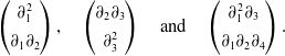 \begin{equation}\begin{pmatrix} \partial_1^2 \\[4pt] \partial_1 \partial_2 \end{pmatrix} , \quad \begin{pmatrix} \partial_2 \partial_3 \\[4pt] \partial_3^2 \end{pmatrix} \quad {\textrm{and}} \quad \begin{pmatrix} \partial_1^2 \partial_3 \\[4pt] \partial_1 \partial_2 \partial_4 \end{pmatrix} .\end{equation}
The system (1.8) corresponds to the submodule of
 $R^2$
that is generated by these three vectors.
$R^2$
that is generated by these three vectors.
We shall study PDE that describe vector-valued functions from n-space to k-space. To this end, we need to specify a space
 $\mathcal{F}$
of sufficiently differentiable functions such that
$\mathcal{F}$
of sufficiently differentiable functions such that
 $\mathcal{F}^k$
contains our solutions. The scalar-valued functions in
$\mathcal{F}^k$
contains our solutions. The scalar-valued functions in
 $\mathcal{F}$
are either real-valued functions
$\mathcal{F}$
are either real-valued functions
 $\psi\,:\,\Omega \rightarrow \mathbb{R}$
or complex-valued functions
$\psi\,:\,\Omega \rightarrow \mathbb{R}$
or complex-valued functions
 $\psi\,:\,\Omega \rightarrow \mathbb{C}$
, where
$\psi\,:\,\Omega \rightarrow \mathbb{C}$
, where
 $\Omega$
is a suitable subset of
$\Omega$
is a suitable subset of
 $\mathbb{R}^n$
or
$\mathbb{R}^n$
or
 $\mathbb{C}^n$
. Later we will be more specific about the choice of
$\mathbb{C}^n$
. Later we will be more specific about the choice of
 $\mathcal{F}$
. One requirement is that the space
$\mathcal{F}$
. One requirement is that the space
 $\mathcal{F}^k$
should contain the exponential functions
$\mathcal{F}^k$
should contain the exponential functions
 \begin{equation} q({\bf z}) \cdot {\textrm{exp}}( {\bf u}^t {\bf z}) = q(z_1,\ldots,z_n) \cdot {\textrm{exp}}( u_1 z_1 + \cdots + u_n z_n).\end{equation}
Here
 ${\bf u} \in \mathbb{C}^n$
and q is any vector of length k whose entries are polynomials in n unknowns.
${\bf u} \in \mathbb{C}^n$
and q is any vector of length k whose entries are polynomials in n unknowns.
Remark 2.1 (
 $k=1$
) A differential operator
$k=1$
) A differential operator
 $p(\partial) $
in R annihilates the function
$p(\partial) $
in R annihilates the function
 ${\textrm{exp}}({\bf u}^t {\bf z})$
if and only if
${\textrm{exp}}({\bf u}^t {\bf z})$
if and only if
 $p({\bf u}) = 0$
. This is the content of [Reference Michałek and Sturmfels27, Lemma 3.25]. See also Lemma 3.26. If
$p({\bf u}) = 0$
. This is the content of [Reference Michałek and Sturmfels27, Lemma 3.25]. See also Lemma 3.26. If
 $p(\partial)$
annihilates a function
$p(\partial)$
annihilates a function
 $ q({\bf z}) \cdot {\textrm{exp}}( {\bf u}^t {\bf z})$
, where q is a polynomial of positive degree, then u is a point of higher multiplicity on the hypersurface
$ q({\bf z}) \cdot {\textrm{exp}}( {\bf u}^t {\bf z})$
, where q is a polynomial of positive degree, then u is a point of higher multiplicity on the hypersurface
 $\{ p = 0 \}$
. In the case
$\{ p = 0 \}$
. In the case
 $n=1$
, when p is the characteristic polynomial (1.3), we have a solution basis of exponential functions (1.2).
$n=1$
, when p is the characteristic polynomial (1.3), we have a solution basis of exponential functions (1.2).
Another requirement for the space
 $\mathcal{F}$
is that it is closed under differentiation. In other words, if
$\mathcal{F}$
is that it is closed under differentiation. In other words, if
 $\phi = \phi(z_1,\ldots,z_n)$
lies in
$\phi = \phi(z_1,\ldots,z_n)$
lies in
 $\mathcal{F}$
, then so does
$\mathcal{F}$
, then so does
 $\partial_i \bullet \phi = \dfrac{\partial \phi}{\partial z_i}$
for
$\partial_i \bullet \phi = \dfrac{\partial \phi}{\partial z_i}$
for
 $i=1,2,\ldots,n$
. The elements of
$i=1,2,\ldots,n$
. The elements of
 $\mathcal{F}^k$
are vector-valued functions
$\mathcal{F}^k$
are vector-valued functions
 $\psi = \psi({\bf z})$
. Their coordinates
$\psi = \psi({\bf z})$
. Their coordinates
 $\psi_i$
are scalar-valued functions in
$\psi_i$
are scalar-valued functions in
 $\mathcal{F}$
. All in all,
$\mathcal{F}$
. All in all,
 $\mathcal{F}$
should be large, in the sense that it furnishes enough solutions. Formulated algebraically, we want
$\mathcal{F}$
should be large, in the sense that it furnishes enough solutions. Formulated algebraically, we want
 $\mathcal{F}$
to be an injective R-module [Reference Lomadze25]. A more precise desideratum, formulated by Oberst [Reference Oberst28–Reference Oberst30], is that
$\mathcal{F}$
to be an injective R-module [Reference Lomadze25]. A more precise desideratum, formulated by Oberst [Reference Oberst28–Reference Oberst30], is that
 $\mathcal{F}$
should be an injective cogenerator.
$\mathcal{F}$
should be an injective cogenerator.
Examples of injective cogenerators include the ring
 $\mathbb{C}[[z_1,\ldots,z_n]]$
of formal power series, the space
$\mathbb{C}[[z_1,\ldots,z_n]]$
of formal power series, the space
 $C^\infty(\mathbb{R}^n)$
of smooth complex-valued functions over
$C^\infty(\mathbb{R}^n)$
of smooth complex-valued functions over
 $\mathbb{R}^n$
, or more generally, the space
$\mathbb{R}^n$
, or more generally, the space
 $\mathcal{D}'(\mathbb{R}^n)$
of complex-valued distributions on
$\mathcal{D}'(\mathbb{R}^n)$
of complex-valued distributions on
 $\mathbb{R}^n$
. If
$\mathbb{R}^n$
. If
 $\Omega $
is any open convex domain in
$\Omega $
is any open convex domain in
 $\mathbb{R}^n$
, then we can also take
$\mathbb{R}^n$
, then we can also take
 $\mathcal{F}$
to be
$\mathcal{F}$
to be
 $C^\infty(\Omega)$
or
$C^\infty(\Omega)$
or
 $\mathcal{D}'(\Omega)$
. In this paper, we focus on algebraic methods. Analytic difficulties are mostly swept under the rug.
$\mathcal{D}'(\Omega)$
. In this paper, we focus on algebraic methods. Analytic difficulties are mostly swept under the rug.
Our PDE are elements in the free R-module
 $R^k$
, that is, they are column vectors of length k whose entries are polynomials in
$R^k$
, that is, they are column vectors of length k whose entries are polynomials in
 $\partial = (\partial_1,\ldots,\partial_n)$
. Such a vector acts on
$\partial = (\partial_1,\ldots,\partial_n)$
. Such a vector acts on
 $\mathcal{F}^k$
by coordinate-wise application of the differential operator and then adding up the results in
$\mathcal{F}^k$
by coordinate-wise application of the differential operator and then adding up the results in
 $\mathcal{F}$
. In this manner, each element in
$\mathcal{F}$
. In this manner, each element in
 $R^k$
defines an R-linear map
$R^k$
defines an R-linear map
 $\mathcal{F}^k \rightarrow \mathcal{F}$
. For instance, the third vector in (2.1) is an element in
$\mathcal{F}^k \rightarrow \mathcal{F}$
. For instance, the third vector in (2.1) is an element in
 $R^2$
that acts on functions
$R^2$
that acts on functions
 $\psi \,:\, \mathbb{R}^4 \rightarrow \mathbb{C}^2$
in
$\psi \,:\, \mathbb{R}^4 \rightarrow \mathbb{C}^2$
in
 $\mathcal{F}^2$
as follows:
$\mathcal{F}^2$
as follows:
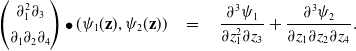 \begin{equation}\begin{pmatrix} \partial_1^2 \partial_3 \\[4pt] \partial_1 \partial_2 \partial_4 \end{pmatrix} \bullet(\psi_1 ({\bf z} ) ,\psi_2({\bf z})) \quad = \quad \frac{\partial^3 \psi_1}{ \partial z_1^2 \partial z_3} + \frac{\partial^3 \psi_2}{ \partial z_1 \partial z_2 \partial z_4}.\end{equation}
The right-hand side is a scalar-valued function
 $\mathbb{R}^4 \rightarrow \mathbb{C}$
, that is, it is an element of
$\mathbb{R}^4 \rightarrow \mathbb{C}$
, that is, it is an element of
 $\mathcal{F}$
.
$\mathcal{F}$
.
Our systems of PDE are submodules M of the free module
 $R^k$
. By Hilbert’s Basis Theorem, every module M is finitely generated, so we can write
$R^k$
. By Hilbert’s Basis Theorem, every module M is finitely generated, so we can write
 $M = {\textrm{image}}_R(A)$
, where A is a
$M = {\textrm{image}}_R(A)$
, where A is a
 $k \times l$
matrix with entries in R. Each column of A is a generator of M, and it defines a differential operator that maps
$k \times l$
matrix with entries in R. Each column of A is a generator of M, and it defines a differential operator that maps
 $\mathcal{F}^k$
to
$\mathcal{F}^k$
to
 $\mathcal{F}$
. The solution space to the PDE given by M equals
$\mathcal{F}$
. The solution space to the PDE given by M equals
 \begin{equation}{\textrm{Sol}}(M) \,:\!=\, \bigl\{ \psi \in \mathcal{F}^k \,:\, m \bullet \psi = 0\ \hbox{for all} \ m \in M \bigr\}.\end{equation}
It suffices to take the operators m from a generating set of M, such as the l columns of A. The case
 $k=1$
is of special interest, since we often consider PDE for scalar-valued functions. In that case, the submodule is an ideal in the polynomial ring R, and we denote this by I. The solution space
$k=1$
is of special interest, since we often consider PDE for scalar-valued functions. In that case, the submodule is an ideal in the polynomial ring R, and we denote this by I. The solution space
 ${\textrm{Sol}}(I)$
of the ideal
${\textrm{Sol}}(I)$
of the ideal
 $I \subseteq R$
is the set of functions
$I \subseteq R$
is the set of functions
 $\phi$
in
$\phi$
in
 $\mathcal{F}$
such that
$\mathcal{F}$
such that
 $p(\partial) \bullet \phi = 0 $
for all
$p(\partial) \bullet \phi = 0 $
for all
 $p \in I$
. Thus, ideals are instances of modules, with their own notation.
$p \in I$
. Thus, ideals are instances of modules, with their own notation.
The solution spaces
 ${\textrm{Sol}}(M)$
and
${\textrm{Sol}}(M)$
and
 ${\textrm{Sol}}(I)$
are
${\textrm{Sol}}(I)$
are
 $\mathbb{C}$
-vector spaces and R-modules. Indeed, any
$\mathbb{C}$
-vector spaces and R-modules. Indeed, any
 $\mathbb{C}$
-linear combination of solutions is again a solution. The R-module action means applying the same differential operator
$\mathbb{C}$
-linear combination of solutions is again a solution. The R-module action means applying the same differential operator
 $p(\partial)$
to each coordinate, which leads to another vector in
$p(\partial)$
to each coordinate, which leads to another vector in
 $\mathcal{F}^k$
. This action takes solutions to solutions because the ring of differential operators with constant coefficients
$\mathcal{F}^k$
. This action takes solutions to solutions because the ring of differential operators with constant coefficients
 $R = \mathbb{C}[\partial_1,\ldots,\partial_n]$
is commutative.
$R = \mathbb{C}[\partial_1,\ldots,\partial_n]$
is commutative.
The purpose of this paper is to present practical methods for the following task:
 \begin{equation} \begin{matrix}{ Given\, a\, k \times l\, matrix\, A \,with\, entries\, in\, R = K[\partial_1,\ldots,\partial_n],\, compute\, a\, good} \\[4pt]{ representation\, for\, the\, solution\, space\, {\textrm{Sol}}(M) \,of\, the\, module\, M = {\textrm{image}}_R(A).}\end{matrix}\end{equation}
If
 $k=1$
then we consider the ideal I generated by the entries of A and we compute
$k=1$
then we consider the ideal I generated by the entries of A and we compute
 ${\textrm{Sol}}(I)$
.
${\textrm{Sol}}(I)$
.
This raises the question of what a “good representation” means. The formulas in (1.2), (1.5), (1.9) and (1.11) are definitely good. They guide us to what is desirable. Our general answer stems from the following important result at the crossroads of analysis and algebra. It involves two sets of unknowns
 ${\bf z} = (z_1,\ldots,z_n)$
and
${\bf z} = (z_1,\ldots,z_n)$
and
 ${\bf x}= (x_1,\ldots,x_n)$
. Here x gives coordinates on certain irreducible varieties
${\bf x}= (x_1,\ldots,x_n)$
. Here x gives coordinates on certain irreducible varieties
 $V_i$
in
$V_i$
in
 $\mathbb{C}^n$
that are parameter spaces for solutions. Our solutions
$\mathbb{C}^n$
that are parameter spaces for solutions. Our solutions
 $\psi$
are functions in z. We take
$\psi$
are functions in z. We take
 $\mathcal{F} = C^\infty(\Omega)$
where
$\mathcal{F} = C^\infty(\Omega)$
where
 $\Omega \subset \mathbb{R}^n$
is open, convex, and bounded.
$\Omega \subset \mathbb{R}^n$
is open, convex, and bounded.
Theorem 2.2 (Ehrenpreis--Palamodov Fundamental Principle). Consider a module
 $M \subseteq R^k$
, representing linear PDE for a function
$M \subseteq R^k$
, representing linear PDE for a function
 $\psi\,:\, \Omega \rightarrow \mathbb{C}^k$
. There exist irreducible varieties
$\psi\,:\, \Omega \rightarrow \mathbb{C}^k$
. There exist irreducible varieties
 $V_1,\ldots,V_s$
in
$V_1,\ldots,V_s$
in
 $\mathbb{C}^n$
and finitely many vectors
$\mathbb{C}^n$
and finitely many vectors
 $B_{ij}$
of polynomials in 2n unknowns
$B_{ij}$
of polynomials in 2n unknowns
 $({\bf x},{\bf z})$
, all independent of the set
$({\bf x},{\bf z})$
, all independent of the set
 $\Omega$
, such that any solution
$\Omega$
, such that any solution
 $\psi \in \mathcal{F}$
admits an integral representation
$\psi \in \mathcal{F}$
admits an integral representation
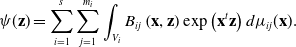 \begin{equation} \psi(\mathbf{z}) = \sum_{i=1}^s \sum_{j=1}^{m_i} \int_{V_i} B_{ij} \left(\mathbf{x},\mathbf{z}\right) \exp\left( \mathbf{x}^t \mathbf{z} \right) d\mu_{ij} (\mathbf{x}).\end{equation}
Here
 $m_i$
is a certain invariant of
$m_i$
is a certain invariant of
 $(M,V_i)$
and each
$(M,V_i)$
and each
 $\mu_{ij}$
is a bounded measure supported on the variety
$\mu_{ij}$
is a bounded measure supported on the variety
 $V_i $
.
$V_i $
.
Theorem 2.2 appears in different forms in the books by Björk [Reference Björk7, Theorem 8.1.3], Ehrenpreis [Reference Ehrenpreis17], Hörmander [Reference Hörmander23, Section 7.7], and Palamodov [Reference Palamodov32]. Other references with different emphases include [Reference Berndtsson and Passare5, Reference Lomadze25, Reference Oberst29]. For a perspective from commutative algebra see [Reference Cid-Ruiz, Homs and Sturmfels11, Reference Cid-Ruiz and Sturmfels12].
In the next sections, we will study the ingredients in Theorem 2.2. Given the module M, we compute each associated variety
 $V_i$
, the arithmetic length
$V_i$
, the arithmetic length
 $m_i$
of M along
$m_i$
of M along
 $V_i$
, and the Noetherian multipliers
$V_i$
, and the Noetherian multipliers
 $B_{i,1},B_{i,2},\ldots,B_{i,m_i}$
. We shall see that not all n of the unknowns
$B_{i,1},B_{i,2},\ldots,B_{i,m_i}$
. We shall see that not all n of the unknowns
 $z_1,\ldots,z_n$
appear in the polynomials
$z_1,\ldots,z_n$
appear in the polynomials
 $B_{i,j}$
but only a subset of
$B_{i,j}$
but only a subset of
 ${\textrm{codim}}(V_i)$
of them.
${\textrm{codim}}(V_i)$
of them.
The most basic example is the ODE in (1.1), with
 $l=n=k=1$
. Here
$l=n=k=1$
. Here
 $V_i = \{u_i\}$
is the ith root of the polynomial (1.3), which has multiplicity
$V_i = \{u_i\}$
is the ith root of the polynomial (1.3), which has multiplicity
 $m_i$
, and
$m_i$
, and
 $B_{i,j} = z^{j-1}$
. The measure
$B_{i,j} = z^{j-1}$
. The measure
 $\mu_{ij}$
is a scaled Dirac measure on
$\mu_{ij}$
is a scaled Dirac measure on
 $u_i$
, so the integrals in (2.6) are multiples of the basis functions (1.2).
$u_i$
, so the integrals in (2.6) are multiples of the basis functions (1.2).
In light of Theorem 2.2, we now refine our computational task in (2.5) as follows:
 \begin{equation} \begin{matrix}{ Given \,a \,k \times l\, matrix \,A\, with\, entries\, in\, R = K[\partial_1,\ldots,\partial_n],\ \ compute\, the\, varieties\, V_i} \\[4pt] { and\, the\, Noetherian\, multipliers\, B_{ij}({\bf x},{\bf z}).\ \ This\, encodes\, {\textrm{Sol}}(M)\, for\, M = {\textrm{image}}_R(A).}\end{matrix}\end{equation}
In our introductory examples, we gave formulas for the general solution, namely (1.5) and (1.9). We claim that such formulas can be read off from the integrals in (2.6). For instance, for the wave equation (1.4), we have
 $s=2$
,
$s=2$
,
 $B_{1,1} = B_{1,2} = 1$
, and (1.5) is obtained by integrating
$B_{1,1} = B_{1,2} = 1$
, and (1.5) is obtained by integrating
 ${\textrm{exp}}( {\bf x}^t {\bf z})$
against measures
${\textrm{exp}}( {\bf x}^t {\bf z})$
against measures
 $ d\mu_{i1}({\bf x})$
on two lines
$ d\mu_{i1}({\bf x})$
on two lines
 $V_1$
and
$V_1$
and
 $V_2$
in
$V_2$
in
 $ \mathbb{C}^2$
. For the system (1.8), we find
$ \mathbb{C}^2$
. For the system (1.8), we find
 $s=6$
, with
$s=6$
, with
 $m_1=m_2=m_3=1$
and
$m_1=m_2=m_3=1$
and
 $m_4=m_5=m_6=2$
, and the nine integrals in (2.6) translate into (1.9). We shall explain such a translation in full detail for two other examples.
$m_4=m_5=m_6=2$
, and the nine integrals in (2.6) translate into (1.9). We shall explain such a translation in full detail for two other examples.
Example 2.3 (
 $n=3,k=1,l=2$
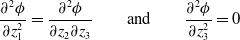
) The ideal
$n=3,k=1,l=2$
) The ideal
 $I = \langle \partial_1^2 - \partial_2 \partial_3, \partial_3^2 \rangle $
represents the PDE
$I = \langle \partial_1^2 - \partial_2 \partial_3, \partial_3^2 \rangle $
represents the PDE
 \begin{equation} \frac{\partial^2 \phi}{\partial z_1^2} = \frac{\partial^2 \phi} {\partial z_2 \partial z_3}\qquad {\textrm{and}} \qquad \frac{\partial^2 \phi}{\partial z_3^2} = 0\end{equation}
for a scalar-valued function
 $\phi = \phi(z_1,z_2,z_3)$
. This is [Reference Chen, Härkönen, Krone and Leykin10, Example 4.2]. A Macaulay2 computation as in Section 5 shows that
$\phi = \phi(z_1,z_2,z_3)$
. This is [Reference Chen, Härkönen, Krone and Leykin10, Example 4.2]. A Macaulay2 computation as in Section 5 shows that
 $s=1, m_1 =4$
. It reveals the Noetherian multipliers
$s=1, m_1 =4$
. It reveals the Noetherian multipliers
 \begin{equation*} B_1 = 1, B_2 = z_1, B_3 = z_1^2 x_2 + 2 z_3, B_4 = z_1^3 x_2 + 6 z_1 z_3 . \end{equation*}
Arbitrary functions
 $f(z_2) = \int {\textrm{exp}}( t z_2 ) dt$
are obtained by integrating against suitable measures on the line
$f(z_2) = \int {\textrm{exp}}( t z_2 ) dt$
are obtained by integrating against suitable measures on the line
 $V_1= \{ (0,t,0) \,:\,t \in \mathbb{C} \} \subset \mathbb{C}^3$
. Their derivatives are found by differentiating under the integral sign, namely
$V_1= \{ (0,t,0) \,:\,t \in \mathbb{C} \} \subset \mathbb{C}^3$
. Their derivatives are found by differentiating under the integral sign, namely
 $f'(z_2) = \int t \cdot {\textrm{exp}}( t z_2 )dt$
. Consider four functions a,b,c,d, each specified by a different measure. Thus, the sum of the four integrals in (2.6) evaluates to
$f'(z_2) = \int t \cdot {\textrm{exp}}( t z_2 )dt$
. Consider four functions a,b,c,d, each specified by a different measure. Thus, the sum of the four integrals in (2.6) evaluates to
 \begin{equation} \phi({\bf z}) = a(z_2) + z_1 b(z_2) + ( z_1^2 c'(z_2) + 2 z_3 c(z_2) ) + ( z_1^3 d'(z_2) + 6 z_1z_3 d(z_2)).\end{equation}
According to Ehrenpreis–Palamodov, this sum is the general solution of the PDE (2.8).
Our final example uses concepts from primary decomposition, to be reviewed in Section 3.
Example 2.4 (
 $n=4,k=2,l=3$
). Let
$n=4,k=2,l=3$
). Let
 $M \subset R^4$
be the module generated by the columns of
$M \subset R^4$
be the module generated by the columns of
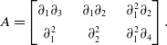 \begin{equation} A = \begin{bmatrix} \partial_{1} \partial_{3} & \quad\partial_{1} \partial_{2} & \quad\partial_{1}^2 \partial_{2} \\[4pt] \partial_{1}^2 & \quad\partial_{2}^2 & \quad\partial_{1}^2 \partial_{4} \end{bmatrix}. \end{equation}
Computing
 ${\textrm{Sol}}(M)$
means solving
${\textrm{Sol}}(M)$
means solving
 $ \dfrac{\partial^2 \psi_1}{\partial z_1 \partial z_3} + \dfrac{\partial^2 \psi_2}{\partial z_1^2} = \dfrac{\partial^2 \psi_1}{\partial z_1 \partial z_2} + \dfrac{\partial^2 \psi_2}{\partial z_2^2} = \dfrac{\partial^3 \psi_1}{\partial z_1^2 \partial z_2} + \dfrac{\partial^3 \psi_2}{\partial z_1^2 \partial z_4} =0$
. Two solutions are
$ \dfrac{\partial^2 \psi_1}{\partial z_1 \partial z_3} + \dfrac{\partial^2 \psi_2}{\partial z_1^2} = \dfrac{\partial^2 \psi_1}{\partial z_1 \partial z_2} + \dfrac{\partial^2 \psi_2}{\partial z_2^2} = \dfrac{\partial^3 \psi_1}{\partial z_1^2 \partial z_2} + \dfrac{\partial^3 \psi_2}{\partial z_1^2 \partial z_4} =0$
. Two solutions are
 $\psi({\bf z}) = \bigl(\phi(z_2,z_3,z_4) , 0\bigr)$
and
$\psi({\bf z}) = \bigl(\phi(z_2,z_3,z_4) , 0\bigr)$
and
 $\psi({\bf z}) = {\textrm{exp}}(s^2 t z_1 + s t^2 z_2 + s^3 z_3 + t^3 z_4) \cdot \bigl( t , -s \bigr)$
.
$\psi({\bf z}) = {\textrm{exp}}(s^2 t z_1 + s t^2 z_2 + s^3 z_3 + t^3 z_4) \cdot \bigl( t , -s \bigr)$
.
We apply Theorem 2.2 to derive the general solution to (2.10). The module M has six associated primes, namely
 $P_1 = \langle \partial_{1} \rangle$
,
$P_1 = \langle \partial_{1} \rangle$
,
 $P_2 = \langle \partial_{2}, \partial_{4} \rangle $
,
$P_2 = \langle \partial_{2}, \partial_{4} \rangle $
,
 $P_3 = \langle \partial_{2}, \partial_{3} \rangle $
,
$P_3 = \langle \partial_{2}, \partial_{3} \rangle $
,
 $P_4 = \langle \partial_{1}, \partial_{3} \rangle $
,
$P_4 = \langle \partial_{1}, \partial_{3} \rangle $
,
 $P_5 = \langle \partial_{1}, \partial_{2} \rangle $
, and
$P_5 = \langle \partial_{1}, \partial_{2} \rangle $
, and
 $P_6 = \langle \partial_{1}^2 - \partial_2 \partial_3, \partial_1 \partial_2 - \partial_3 \partial_4,\partial_2^2 - \partial_1 \partial_4 \rangle $
. Four of them are minimal and two are embedded. We find that
$P_6 = \langle \partial_{1}^2 - \partial_2 \partial_3, \partial_1 \partial_2 - \partial_3 \partial_4,\partial_2^2 - \partial_1 \partial_4 \rangle $
. Four of them are minimal and two are embedded. We find that
 $m_1 = m_2 = m_3 = m_4 = m_6 = 1$
and
$m_1 = m_2 = m_3 = m_4 = m_6 = 1$
and
 $m_5 = 4$
. A minimal primary decomposition
$m_5 = 4$
. A minimal primary decomposition
 \begin{equation} M = M_1 \cap M_2 \cap M_3 \cap M_4 \cap M_5 \cap M_6 \end{equation}
is given by the following primary submodules of
 $R^4$
, each of which contains M:
$R^4$
, each of which contains M:
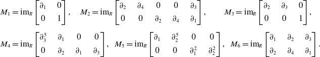 \begin{align*} M_1 & = {\textrm{im}}_R \begin{bmatrix} \partial_1 & \quad 0 \\[4pt] 0 & \quad 1 \end{bmatrix},\quad M_2 = {\textrm{im}}_R \begin{bmatrix} \partial_2 & \quad \partial_4 & \quad 0 & \quad 0 & \quad \partial_3 \\[4pt] 0 & \quad 0 & \quad \partial_2 & \quad \partial_4 & \quad \partial_1\end{bmatrix},\qquad M_3 = {\textrm{im}}_R \begin{bmatrix} \partial_2 & \quad \partial_3 & \quad 0 \\[4pt] 0 & \quad 0 & \quad 1 \end{bmatrix},\\[5pt]M_4 & = {\textrm{im}}_R \begin{bmatrix} \partial_3^5 & \quad \partial_1 & \quad 0 & \quad 0 \\[4pt] 0 & \quad \partial_2 & \quad \partial_1 & \quad \partial_3 \end{bmatrix},\ \ M_5 = {\textrm{im}}_R \begin{bmatrix} \partial_1 & \quad \partial_2^5 & \quad 0 & \quad 0 \\[4pt] 0 & \quad 0 & \quad \partial_1^2 & \quad \partial_2^2 \end{bmatrix},\ \ M_6 = {\textrm{im}}_R \begin{bmatrix}\partial_1 & \quad \partial_2 & \quad \partial_3 \\[4pt]\partial_2 & \quad \partial_4 & \quad \partial_1\end{bmatrix}. \end{align*}
The number of Noetherian multipliers
 $B_{ij}$
is
$B_{ij}$
is
 $\sum_{i=1}^6 m_i = 9$
. We choose them to be
$\sum_{i=1}^6 m_i = 9$
. We choose them to be
 \begin{equation*} B_{1,1} {=} \begin{bmatrix} 1 \\[4pt] 0 \end{bmatrix} , B_{2,1} {=} \begin{bmatrix} \phantom{-}x_1 \\[4pt] -x_3 \end{bmatrix} , B_{3,1} {=} \begin{bmatrix} 1 \\[4pt] 0 \end{bmatrix} , B_{4,1} = \begin{bmatrix} x_2 z_1 \\[4pt] -1 \end{bmatrix} , B_{5,i} = \begin{bmatrix} 0 \\[4pt] z_1 z_2 \end{bmatrix} , \begin{bmatrix} 0 \\[4pt] z_1 \end{bmatrix} , \begin{bmatrix} 0 \\[4pt] z_2 \end{bmatrix} , \begin{bmatrix} 0 \\[4pt] 1 \end{bmatrix} , B_{6,1} = \begin{bmatrix} \phantom{-}x_4 \\[4pt] -x_2 \end{bmatrix}.\end{equation*}
These nine vectors describe all solutions to our PDE. For instance,
 $B_{3,1}$
gives the solutions
$B_{3,1}$
gives the solutions
 $ \Big[\begin{array}{c} \alpha(z_1,z_4) \\[4pt] 0 \end{array}\Big]$
, and
$ \Big[\begin{array}{c} \alpha(z_1,z_4) \\[4pt] 0 \end{array}\Big]$
, and
 $B_{5,1}$
gives the solutions
$B_{5,1}$
gives the solutions
 $ \Big[\begin{array}{c} 0 \\[4pt] z_1 z_2 \beta(z_3,z_4) \end{array}\Big]$
, where
$ \Big[\begin{array}{c} 0 \\[4pt] z_1 z_2 \beta(z_3,z_4) \end{array}\Big]$
, where
 $\alpha,\beta$
are bivariate functions. Furthermore,
$\alpha,\beta$
are bivariate functions. Furthermore,
 $B_{1,1}$
and
$B_{1,1}$
and
 $B_{6,1}$
encode the two families of solutions mentioned after (2.10).
$B_{6,1}$
encode the two families of solutions mentioned after (2.10).
For the latter, we note that
 $V_6 = V(P_6) $
is the surface in
$V_6 = V(P_6) $
is the surface in
 $\mathbb{C}^4$
with parametric representation
$\mathbb{C}^4$
with parametric representation
 $(x_1,x_2,x_3,x_4) = (s^2 t, st^2, s^3,t^3)$
for
$(x_1,x_2,x_3,x_4) = (s^2 t, st^2, s^3,t^3)$
for
 $s,t \in \mathbb{C}$
. This surface is the cone over the twisted cubic curve, in the same notation as in [Reference Cid-Ruiz, Homs and Sturmfels11, Section 1]. The kernel under the integral in (2.6) equals
$s,t \in \mathbb{C}$
. This surface is the cone over the twisted cubic curve, in the same notation as in [Reference Cid-Ruiz, Homs and Sturmfels11, Section 1]. The kernel under the integral in (2.6) equals
 \begin{equation*} \begin{bmatrix} \phantom{-}x_4 \\[4pt] -x_2 \end{bmatrix}{\textrm{exp}}\bigl(x_1 z_1 + x_2 z_2 + x_3 z_3 + x_4 z_4\bigr) \quad = \quad t^2 \begin{bmatrix} \phantom{-} t \\[4pt] - s \end{bmatrix} {\textrm{exp}}\bigl( s^2t z_1 + st^2 z_2 + s^3 z_3 + t^3 z_4 \bigr).\end{equation*}
This is a solution to
 $M_6$
, and hence to M, for any values of s and t. Integrating the left- hand side over
$M_6$
, and hence to M, for any values of s and t. Integrating the left- hand side over
 ${\bf x} \in V_6$
amounts to integrating the right-hand side over
${\bf x} \in V_6$
amounts to integrating the right-hand side over
 $(s,t) \in \mathbb{C}^2$
. Any such integral is also a solution. Ehrenpreis–Palamodov tells us that these are all the solutions.
$(s,t) \in \mathbb{C}^2$
. Any such integral is also a solution. Ehrenpreis–Palamodov tells us that these are all the solutions.
3. Modules and varieties
Our aim is to offer practical tools for solving PDE. The input is a
 $k \times l$
matrix A with entries in
$k \times l$
matrix A with entries in
 $R = K[\partial_1,\ldots,\partial_n]$
, and
$R = K[\partial_1,\ldots,\partial_n]$
, and
 $M = {\textrm{image}}_R(A)$
is the corresponding submodule of
$M = {\textrm{image}}_R(A)$
is the corresponding submodule of
 $R^k = \bigoplus_{j=1}^k Re_j$
. The output is the description of
$R^k = \bigoplus_{j=1}^k Re_j$
. The output is the description of
 ${\textrm{Sol}}(M)$
sought in (2.7). That description is unique up to basis change, in the sense of [Reference Cid-Ruiz and Sturmfels12, Remark 3.8], by the discussion in Section 4. Our method is implemented in a Macaulay2 command, called solvePDE and to be described in Section 5.
${\textrm{Sol}}(M)$
sought in (2.7). That description is unique up to basis change, in the sense of [Reference Cid-Ruiz and Sturmfels12, Remark 3.8], by the discussion in Section 4. Our method is implemented in a Macaulay2 command, called solvePDE and to be described in Section 5.
We now explain the ingredients of Theorem 2.2 coming from commutative algebra (cf. [Reference Eisenbud18]). For a vector
 $m \in R^k$
, the quotient
$m \in R^k$
, the quotient
 $(M\,:\,m)$
is the ideal
$(M\,:\,m)$
is the ideal
 $\{f \in R \,:\, fm \in M\}$
. A prime ideal
$\{f \in R \,:\, fm \in M\}$
. A prime ideal
 $P_i \subseteq R$
is associated to M if there exists
$P_i \subseteq R$
is associated to M if there exists
 $m \in R^k$
such that
$m \in R^k$
such that
 $(M\,:\,m) = P_i$
. Since R is Noetherian, the list of associated primes of M is finite, say
$(M\,:\,m) = P_i$
. Since R is Noetherian, the list of associated primes of M is finite, say
 $P_1,\ldots,P_s$
. If
$P_1,\ldots,P_s$
. If
 $s=1$
then the module M is called primary or
$s=1$
then the module M is called primary or
 $P_1$
-primary. A primary decomposition of M is a list of primary submodules
$P_1$
-primary. A primary decomposition of M is a list of primary submodules
 $M_1,\ldots,M_s \subseteq R^k$
where
$M_1,\ldots,M_s \subseteq R^k$
where
 $M_i$
is
$M_i$
is
 $P_i$
-primary and
$P_i$
-primary and
 $ M = M_1 \cap M_2 \cap \cdots \cap M_s $
.
$ M = M_1 \cap M_2 \cap \cdots \cap M_s $
.
Primary decomposition is a standard topic in commutative algebra. It is usually presented for ideals
 $(k=1)$
, as in [Reference Michałek and Sturmfels27, Chapter 3]. The case of modules is analogous. The latest version of Macaulay2 has an implementation of primary decomposition for modules, as described in [Reference Chen and Cid-Ruiz9, Section 2]. Given M, the primary module
$(k=1)$
, as in [Reference Michałek and Sturmfels27, Chapter 3]. The case of modules is analogous. The latest version of Macaulay2 has an implementation of primary decomposition for modules, as described in [Reference Chen and Cid-Ruiz9, Section 2]. Given M, the primary module
 $M_i$
is not unique if
$M_i$
is not unique if
 $P_i$
is an embedded prime.
$P_i$
is an embedded prime.
The contribution of the primary module
 $M_i$
to M is quantified by a positive integer
$M_i$
to M is quantified by a positive integer
 $m_i$
, called the arithmetic length of M along
$m_i$
, called the arithmetic length of M along
 $P_i$
. To define this, we consider the localization
$P_i$
. To define this, we consider the localization
 $(R_{P_i})^k/M_{P_i}$
. This is a module over the local ring
$(R_{P_i})^k/M_{P_i}$
. This is a module over the local ring
 $R_{P_i}$
. The arithmetic length is the length of the largest submodule of finite length in
$R_{P_i}$
. The arithmetic length is the length of the largest submodule of finite length in
 $(R_{P_i})^k/M_{P_i}$
; in symbols,
$(R_{P_i})^k/M_{P_i}$
; in symbols,
 $m_i = {\textrm{length}} \bigl( H^0_{P_i} ((R_{P_i})^k/ M_{P_i})\bigr)$
. The sum
$m_i = {\textrm{length}} \bigl( H^0_{P_i} ((R_{P_i})^k/ M_{P_i})\bigr)$
. The sum
 $m_1 + \cdots + m_s$
is an invariant of the module M, denoted
$m_1 + \cdots + m_s$
is an invariant of the module M, denoted
 ${\textrm{amult}}(M)$
, and known as the arithmetic multiplicity of M. These numbers can be computed in Macaulay2 as in [Reference Cid-Ruiz and Sturmfels12, Remark 5.1]. We return to these invariants in Theorem 4.3.
${\textrm{amult}}(M)$
, and known as the arithmetic multiplicity of M. These numbers can be computed in Macaulay2 as in [Reference Cid-Ruiz and Sturmfels12, Remark 5.1]. We return to these invariants in Theorem 4.3.
To make the connection to Theorem 2.2, we set
 $V_i = V(P_i)$
for
$V_i = V(P_i)$
for
 $i=1,2,\ldots,s$
. Thus,
$i=1,2,\ldots,s$
. Thus,
 $V_i$
is the irreducible variety in
$V_i$
is the irreducible variety in
 $\mathbb{C}^n$
defined by the prime ideal
$\mathbb{C}^n$
defined by the prime ideal
 $P_i$
in
$P_i$
in
 $R = K[\partial_1,\ldots,\partial_n]$
. The integer
$R = K[\partial_1,\ldots,\partial_n]$
. The integer
 $m_i$
is an invariant of the pair
$m_i$
is an invariant of the pair
 $(M,V_i)$
: it measures the thickness of the module M along
$(M,V_i)$
: it measures the thickness of the module M along
 $V_i$
.
$V_i$
.
By taking the union of the irreducible varieties
 $V_i$
we obtain the variety
$V_i$
we obtain the variety
 \begin{equation*} V(M) \quad \,:\!=\, \quad V_1 \cup V_2 \cup \cdots \cup V_s\quad \subset \mathbb{C}^n.\end{equation*}
Algebraists refer to V(M) as the support of M, while analysts call it the characteristic variety of M. The support is generally reducible, with
 $\leq s$
irreducible components. For instance, the module M in Example 2.4 has six associated primes, and an explicit primary decomposition was given in (2.11). However, the support V(M) has only four irreducible components in
$\leq s$
irreducible components. For instance, the module M in Example 2.4 has six associated primes, and an explicit primary decomposition was given in (2.11). However, the support V(M) has only four irreducible components in
 $\mathbb{C}^4$
, namely one hyperplane, two-dimensional planes, and one nonlinear surface (twisted cubic).
$\mathbb{C}^4$
, namely one hyperplane, two-dimensional planes, and one nonlinear surface (twisted cubic).
Remark 3.1. If
 $k=1$
and
$k=1$
and
 $M=I$
, then the support V(M) coincides with the variety V(I) attached as usual to an ideal I, namely the common zero set in
$M=I$
, then the support V(M) coincides with the variety V(I) attached as usual to an ideal I, namely the common zero set in
 $\mathbb{C}^n$
of all polynomials in I.
$\mathbb{C}^n$
of all polynomials in I.
The relationship between modules and ideals mirrors the relationship between PDE for vector-valued functions and related PDE for scalar-valued functions. To pursue this a bit further, we now define two ideals that are naturally associated with a given module
 $M\subseteq R^k$
.
$M\subseteq R^k$
.
The first ideal is the annihilator of the quotient module
 $R^k/M = {\textrm{coker}}_R(A)$
, which is
$R^k/M = {\textrm{coker}}_R(A)$
, which is
 \begin{equation*} I \,:\!=\, {\textrm{Ann}}_R(R^k/M) = \big\{ f \in R \,:\, f m \in M\ \hbox{for all}\ m \in R^k \bigr\} . \end{equation*}
The second is the zeroth Fitting ideal of
 $R^k/M$
, which is the ideal in R generated by the
$R^k/M$
, which is the ideal in R generated by the
 $k \times k$
minors of the presentation matrix A. It is independent of the choice of A, and we write
$k \times k$
minors of the presentation matrix A. It is independent of the choice of A, and we write
 \begin{equation*} J \,:\!=\, {\textrm{Fitt}}_0(R^k/M) = \bigl\langle\hbox{$k \times k$ subdeterminants of A}\bigr\rangle. \end{equation*}
We are interested in the affine varieties in
 $\mathbb{C}^n$
defined by these ideals. They are denoted by V(I) and V(J), respectively. The following is a standard result in commutative algebra.
$\mathbb{C}^n$
defined by these ideals. They are denoted by V(I) and V(J), respectively. The following is a standard result in commutative algebra.
Proposition 3.2. The three varieties above are equal for every submodule M of
 $R^k$
, that is,
$R^k$
, that is,
 \begin{equation} V(M) = V(I) = V(J) \subseteq \mathbb{C}^n. \end{equation}
Proof. This follows from [Reference Eisenbud18, Proposition 20.7].
![]()
Remark 3.3. It can happen that
 ${\textrm{rank}}(A) < k$
, for instance when
${\textrm{rank}}(A) < k$
, for instance when
 $k > l$
. In that case,
$k > l$
. In that case,
 $I = J = \{ 0 \}$
and
$I = J = \{ 0 \}$
and
 $V(M) = \mathbb{C}^n$
. Geometrically, the module M furnishes a coherent sheaf that is supported on the entire space
$V(M) = \mathbb{C}^n$
. Geometrically, the module M furnishes a coherent sheaf that is supported on the entire space
 $\mathbb{C}^n$
. For instance, let
$\mathbb{C}^n$
. For instance, let
 $k=n=2,l=1$
, and
$k=n=2,l=1$
, and
 $A = \displaystyle\binom{\phantom{-}\partial_1}{-\partial_2}$
. The PDE asks for pairs
$A = \displaystyle\binom{\phantom{-}\partial_1}{-\partial_2}$
. The PDE asks for pairs
 $(\psi_1,\psi_2)$
such that
$(\psi_1,\psi_2)$
such that
 $\partial \psi_1 /\partial z_1 = \partial \psi_2 /\partial z_2 $
. We see that
$\partial \psi_1 /\partial z_1 = \partial \psi_2 /\partial z_2 $
. We see that
 $\textrm{Sol}(M)$
consists of all pairs
$\textrm{Sol}(M)$
consists of all pairs
 $\bigl( \partial \alpha/ \partial z_2,\partial \alpha/ \partial z_1 \big)$
, where
$\bigl( \partial \alpha/ \partial z_2,\partial \alpha/ \partial z_1 \big)$
, where
 $\alpha= \alpha(z_1,z_2)$
runs over functions in two variables. In general, the left kernel of A furnishes differential operators for creating solutions to M.
$\alpha= \alpha(z_1,z_2)$
runs over functions in two variables. In general, the left kernel of A furnishes differential operators for creating solutions to M.
The following example shows that (3.1) is not true at the level of schemes (cf. Section 6).
Example 3.4. (
 $n=k=3,l=5$
) Let
$n=k=3,l=5$
) Let
 $R = \mathbb{C}[\partial_1,\partial_2,\partial_3]$
and M the submodule of
$R = \mathbb{C}[\partial_1,\partial_2,\partial_3]$
and M the submodule of
 $R^3$
given by
$R^3$
given by
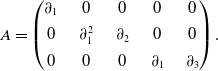 \begin{equation*} A = \begin{pmatrix}\partial_1 & \quad 0 & \quad 0 & \quad 0 & \quad 0 \\[4pt] 0 & \quad \partial_1^2 & \quad \partial_2 & \quad 0 & \quad 0 \\[4pt] 0 & \quad 0 & \quad 0 & \quad \partial_1 & \quad \partial_3 \end{pmatrix} . \end{equation*}
We find
 $I = \langle \partial_1^2, \partial_1 \partial_2 \rangle \supset J = \langle \partial_1^4, \partial_1^3 \partial_3,\partial_1^2 \partial_2 , \partial_1 \partial_2 \partial_3 \rangle$
. The sets of associated primes are
$I = \langle \partial_1^2, \partial_1 \partial_2 \rangle \supset J = \langle \partial_1^4, \partial_1^3 \partial_3,\partial_1^2 \partial_2 , \partial_1 \partial_2 \partial_3 \rangle$
. The sets of associated primes are
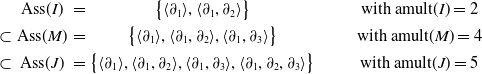 \begin{equation*} \begin{matrix}& \textrm{Ass}(I) & = & \bigl\{ \langle \partial_1 \rangle, \langle \partial_1, \partial_2 \rangle \bigr\}&\qquad & {\textrm{with}}\ {\textrm{amult}}(I) =2 \\[4pt] \subset & \textrm{Ass}(M) & = & \bigl\{ \langle \partial_1 \rangle, \langle \partial_1, \partial_2 \rangle , \langle \partial_1, \partial_3 \rangle \bigr\} & \qquad & {\textrm{with}}\ {\textrm{amult}}(M) = 4 \\[4pt] \subset & \textrm{Ass}(J) & = & \bigl\{ \langle \partial_1 \rangle, \langle \partial_1, \partial_2 \rangle , \langle \partial_1, \partial_3 \rangle, \langle \partial_1, \partial_2, \partial_3 \rangle \bigr\} & \qquad & {\textrm{with}}\ {\textrm{amult}}(J) = 5 \end{matrix} \end{equation*}
The support V(M) is a plane in 3-space, on which I and J define different scheme structures. Our module M defines a coherent sheaf on that plane that lives between these two schemes. We consider the PDE in each of the three cases, we compute the Noetherian multipliers, and from this we derive the general solution. To begin with, functions in
 $ {\textrm{Sol}}(J)$
have the form
$ {\textrm{Sol}}(J)$
have the form
 \begin{equation*} \alpha(z_2,z_3) + z_1 \beta(z_3) + z_1^2 \gamma(z_3) +z_1 \delta(z_2) + c \cdot z_1^3 . \end{equation*}
The first two terms give functions in the subspace
 ${\textrm{Sol}}(I)$
. Elements in
${\textrm{Sol}}(I)$
. Elements in
 ${\textrm{Sol}}(M)$
are vectors
${\textrm{Sol}}(M)$
are vectors
 \begin{equation*} \bigl( \rho(z_2,z_3) , \sigma(z_3) + z_1 \tau(z_3), \omega(z_2) \bigr) . \end{equation*}
These represent all functions
 $\mathbb{C}^3 \rightarrow \mathbb{C}^3$
that satisfy the five PDE given by the matrix A.
$\mathbb{C}^3 \rightarrow \mathbb{C}^3$
that satisfy the five PDE given by the matrix A.
Remark 3.5. The quotient
 $R/I$
embeds naturally into the direct sum of k copies of
$R/I$
embeds naturally into the direct sum of k copies of
 $R^k/M$
, via
$R^k/M$
, via
 $1 \mapsto e_j$
. This implies
$1 \mapsto e_j$
. This implies
 ${\textrm{Ass}}(I) \subseteq {\textrm{Ass}}(M)$
. It would be worthwhile to understand how the differential primary decompositions of I,J and M are related, and to study implications for the solution spaces
${\textrm{Ass}}(I) \subseteq {\textrm{Ass}}(M)$
. It would be worthwhile to understand how the differential primary decompositions of I,J and M are related, and to study implications for the solution spaces
 ${\textrm{Sol}}(I)$
,
${\textrm{Sol}}(I)$
,
 ${\textrm{Sol}}(J)$
, and
${\textrm{Sol}}(J)$
, and
 ${\textrm{Sol}}(M)$
. What relationships hold between these?
${\textrm{Sol}}(M)$
. What relationships hold between these?
Lemma 3.6. Fix a
 $k \times l$
matrix
$k \times l$
matrix
 $A(\partial)$
and its module
$A(\partial)$
and its module
 $M \subseteq R^k$
as above. A point
$M \subseteq R^k$
as above. A point
 ${\bf u}\in \mathbb{C}^n$
lies in V(M) if and only if there exist constants
${\bf u}\in \mathbb{C}^n$
lies in V(M) if and only if there exist constants
 $c_1,\ldots,c_k \in \mathbb{C}$
, not all zero, such that
$c_1,\ldots,c_k \in \mathbb{C}$
, not all zero, such that
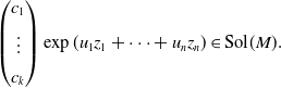 \begin{align} \begin{pmatrix} c_1 \\[4pt] \vdots \\[4pt] c_k \end{pmatrix} \exp(u_1z_1 + \dotsb + u_nz_n) \in \textrm{Sol}(M). \end{align}
More precisely, (3.2) holds if and only if
 $ (c_1,\ldots,c_k) \cdot A({\bf u}) = 0 $
.
$ (c_1,\ldots,c_k) \cdot A({\bf u}) = 0 $
.
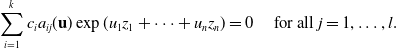
Proof. Let
 $a_{ij}(\partial)$
denote the entries of the matrix
$a_{ij}(\partial)$
denote the entries of the matrix
 $A(\partial)$
. Then (3.2) holds if and only if
$A(\partial)$
. Then (3.2) holds if and only if
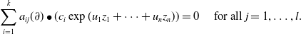 \begin{align*} \sum_{i = 1}^k a_{ij}(\partial) \bullet (c_i \exp(u_1z_1+\dotsb + u_nz_n)) = 0 \quad \text{ for all } j = 1,\ldots, l. \end{align*}
This is equivalent to
 \begin{align*} \sum_{i=1}^k c_i a_{ij}({\bf u}) \exp(u_1z_1+\dotsb + u_nz_n) = 0 \quad \text{ for all } j = 1,\ldots,l. \end{align*}
This condition holds if and only if
 $ (c_1,\ldots,c_k) \cdot A({\bf u}) $
is the zero vector in
$ (c_1,\ldots,c_k) \cdot A({\bf u}) $
is the zero vector in
 $\mathbb{C}^l$
. We conclude that, for any given
$\mathbb{C}^l$
. We conclude that, for any given
 ${\bf u} \in \mathbb{C}^n$
, the previous condition is satisfied for some
${\bf u} \in \mathbb{C}^n$
, the previous condition is satisfied for some
 $c \in \mathbb{C}^k \backslash \{0\}$
if and only if
$c \in \mathbb{C}^k \backslash \{0\}$
if and only if
 ${\textrm{rank}}(A({\bf u})) < k$
if and only if
${\textrm{rank}}(A({\bf u})) < k$
if and only if
 ${\bf u} \in V(M) = V(I)$
. Here we use Proposition 3.2.
${\bf u} \in V(M) = V(I)$
. Here we use Proposition 3.2.
![]()
Here is an alternative way to interpret the characteristic variety of a system of PDE:
Proposition 3.7. The solution space
 $\textrm{Sol}(M)$
contains an exponential solution
$\textrm{Sol}(M)$
contains an exponential solution
 $ q({\bf z}) \cdot {\textrm{exp}}( {\bf u}^t {\bf z}) $
if and only if
$ q({\bf z}) \cdot {\textrm{exp}}( {\bf u}^t {\bf z}) $
if and only if
 ${\bf u} \in V(M)$
. Here q is some vector of k polynomials in n unknowns, as in (2.2).
${\bf u} \in V(M)$
. Here q is some vector of k polynomials in n unknowns, as in (2.2).
Proof. One direction is clear from Lemma 3.6. Next, suppose
 $ q(\mathbf{z}) \exp({\bf u}^t {\bf z}) \in \textrm{Sol}(M)$
. The partial derivative of this function with respect to any unknown
$ q(\mathbf{z}) \exp({\bf u}^t {\bf z}) \in \textrm{Sol}(M)$
. The partial derivative of this function with respect to any unknown
 $z_i$
is also in
$z_i$
is also in
 ${\textrm{Sol}}(M)$
. Hence,
${\textrm{Sol}}(M)$
. Hence,
 \begin{align*} \partial_i \bullet (q({\bf z}) \exp({\bf u}^t {\bf z})) = (\partial_i \bullet q({\bf z})) \exp({\bf u}^t {\bf z})+ u_i q({\bf z}) \exp({\bf u}^t {\bf z}) \in \textrm{Sol}(M) \quad \hbox{for $i=1,\ldots,n$.} \end{align*}
Hence, the exponential function
 $ (\partial_i \bullet q({\bf z})) \exp({\bf u}^t {\bf z})$
is in
$ (\partial_i \bullet q({\bf z})) \exp({\bf u}^t {\bf z})$
is in
 ${\textrm{Sol}}(M)$
. Since the degree of
${\textrm{Sol}}(M)$
. Since the degree of
 $\partial_i \bullet q({\bf z})$
is less than that of
$\partial_i \bullet q({\bf z})$
is less than that of
 $q({\bf z})$
, we can find a sequence
$q({\bf z})$
, we can find a sequence
 $D = \partial_{i_1} \partial_{i_2} \dotsb \partial_{i_s}$
such that
$D = \partial_{i_1} \partial_{i_2} \dotsb \partial_{i_s}$
such that
 $D \bullet q$
is a nonzero constant vector and
$D \bullet q$
is a nonzero constant vector and
 $(D \bullet q) \exp({\bf u}^t {\bf z}) \in \textrm{Sol}(M)$
. Lemma 3.6 now implies that
$(D \bullet q) \exp({\bf u}^t {\bf z}) \in \textrm{Sol}(M)$
. Lemma 3.6 now implies that
 ${\bf u} \in V(M)$
.
${\bf u} \in V(M)$
.
![]()
The solution space
 ${\textrm{Sol}}(M)$
to a submodule
${\textrm{Sol}}(M)$
to a submodule
 $M \subseteq R^k$
is a vector space over
$M \subseteq R^k$
is a vector space over
 $\mathbb{C}$
. It is infinite-dimensional whenever V(M) is a variety of positive dimension. This follows from Lemma 3.6 because there are infinitely many points u in V(M). However, if V(M) is a finite subset of
$\mathbb{C}$
. It is infinite-dimensional whenever V(M) is a variety of positive dimension. This follows from Lemma 3.6 because there are infinitely many points u in V(M). However, if V(M) is a finite subset of
 $\mathbb{C}^n$
, then
$\mathbb{C}^n$
, then
 ${\textrm{Sol}}(M)$
is finite-dimensional. This is the content of the next theorem.
${\textrm{Sol}}(M)$
is finite-dimensional. This is the content of the next theorem.
Theorem 3.8. Consider a module
 $M \subseteq R^k$
, viewed as a system of linear PDE. Its solution space
$M \subseteq R^k$
, viewed as a system of linear PDE. Its solution space
 $\textrm{Sol}(M)$
is finite-dimensional over
$\textrm{Sol}(M)$
is finite-dimensional over
 $\mathbb{C}$
if and only if V(M) has dimension 0. In this case,
$\mathbb{C}$
if and only if V(M) has dimension 0. In this case,
 ${\textrm{dim}}_\mathbb{C} \textrm{Sol}(M) = {\textrm{dim}}_K(R^k/M) = {\textrm{amult}}(M)$
. There is a basis of
${\textrm{dim}}_\mathbb{C} \textrm{Sol}(M) = {\textrm{dim}}_K(R^k/M) = {\textrm{amult}}(M)$
. There is a basis of
 ${\textrm{Sol}}(M)$
given by vectors
${\textrm{Sol}}(M)$
given by vectors
 $ q({\bf z}) {\textrm{exp}}({\bf u}^t {\bf z})$
, where
$ q({\bf z}) {\textrm{exp}}({\bf u}^t {\bf z})$
, where
 ${\bf u} \in V(M)$
and
${\bf u} \in V(M)$
and
 $q({\bf z})$
runs over a finite set of polynomial vectors, whose cardinality is the length of M along the maximal ideal
$q({\bf z})$
runs over a finite set of polynomial vectors, whose cardinality is the length of M along the maximal ideal
 $\langle x_1 - u_1,\ldots,x_n-u_n \rangle$
. There exist polynomial solutions if and only if
$\langle x_1 - u_1,\ldots,x_n-u_n \rangle$
. There exist polynomial solutions if and only if
 $\mathfrak{m} = \langle x_1,\ldots,x_n \rangle$
is an associated prime of M. The polynomial solutions are found by solving the PDE given by the
$\mathfrak{m} = \langle x_1,\ldots,x_n \rangle$
is an associated prime of M. The polynomial solutions are found by solving the PDE given by the
 $\mathfrak{m}$
-primary component of M.
$\mathfrak{m}$
-primary component of M.
Proof. This is the main result in Oberst’s article [Reference Oberst30], proved in the setting of injective cogenerators
 $\mathcal{F}$
. The same statement for
$\mathcal{F}$
. The same statement for
 $\mathcal{F} = C^\infty(\Omega)$
appears in [Reference Björk7, Ch. 8, Theorem 7.1]. The scalar case
$\mathcal{F} = C^\infty(\Omega)$
appears in [Reference Björk7, Ch. 8, Theorem 7.1]. The scalar case
 $(k=1)$
is found in [Reference Michałek and Sturmfels27, Theorem 3.27]. The proof given there uses solutions in the power series ring, which is an injective cogenerator, and it generalizes to modules.
$(k=1)$
is found in [Reference Michałek and Sturmfels27, Theorem 3.27]. The proof given there uses solutions in the power series ring, which is an injective cogenerator, and it generalizes to modules.
![]()
By a polynomial solution we mean a vector
 $q({\bf z})$
whose coordinates are polynomials. The
$q({\bf z})$
whose coordinates are polynomials. The
 $\mathfrak{m}$
-primary component in Theorem 3.8 is computed by a double saturation step. When
$\mathfrak{m}$
-primary component in Theorem 3.8 is computed by a double saturation step. When
 $M=I$
is an ideal, then this double saturation is
$M=I$
is an ideal, then this double saturation is
 $I\,:\,(I\,:\,\mathfrak{m}^\infty)$
, as seen in [Reference Michałek and Sturmfels27, Theorem 3.27]. For submodules M of
$I\,:\,(I\,:\,\mathfrak{m}^\infty)$
, as seen in [Reference Michałek and Sturmfels27, Theorem 3.27]. For submodules M of
 $R^k$
with
$R^k$
with
 $k \geq 2$
, we would compute
$k \geq 2$
, we would compute
 $ M \,:\, {\textrm{Ann}}(R^k / (M \,:\, \mathfrak{m}^\infty) ) $
. The inner colon
$ M \,:\, {\textrm{Ann}}(R^k / (M \,:\, \mathfrak{m}^\infty) ) $
. The inner colon
 $(M\,:\,\mathfrak{m}^\infty)$
is the intersection of all primary components of M whose variety
$(M\,:\,\mathfrak{m}^\infty)$
is the intersection of all primary components of M whose variety
 $V_i$
does not contain the origin 0. It is computed as
$V_i$
does not contain the origin 0. It is computed as
 $(M\,:\,f) = \{m \in R^k\,:\, fm \in M \}$
, where f is a random homogeneous polynomial of large degree. The outer colon is the module
$(M\,:\,f) = \{m \in R^k\,:\, fm \in M \}$
, where f is a random homogeneous polynomial of large degree. The outer colon is the module
 $(M\,:\,g)$
, where g is a general polynomial in the ideal
$(M\,:\,g)$
, where g is a general polynomial in the ideal
 $\textrm{Ann}(R^k/(M\,:\,f))$
. See also [Reference Chen and Cid-Ruiz9, Proposition 2.2].
$\textrm{Ann}(R^k/(M\,:\,f))$
. See also [Reference Chen and Cid-Ruiz9, Proposition 2.2].
It is an interesting problem to identify polynomial solutions when V(M) is no longer finite and to decide whether these are dense in the infinite-dimensional space of all solutions. Here “dense” refers to the topology on
 $\mathcal{F}$
used by Lomadze in [Reference Lomadze26]. The following result gives an algebraic characterization of the closure in
$\mathcal{F}$
used by Lomadze in [Reference Lomadze26]. The following result gives an algebraic characterization of the closure in
 ${\textrm{Sol}}(M)$
of the subspace of polynomial solutions.
${\textrm{Sol}}(M)$
of the subspace of polynomial solutions.
Proposition 3.9. The polynomial solutions are dense in
 ${\textrm{Sol}}(M)$
if and only if the origin 0 lies in every associated variety
${\textrm{Sol}}(M)$
if and only if the origin 0 lies in every associated variety
 $V_i$
of the module M. If this fails, then the topological closure of the space of polynomial solutions
$V_i$
of the module M. If this fails, then the topological closure of the space of polynomial solutions
 $q({\bf z})$
to M is the solution space of
$q({\bf z})$
to M is the solution space of
 $M \,:\, \textrm{Ann}(R^k/(M \,:\, \mathfrak{m}^\infty))$
.
$M \,:\, \textrm{Ann}(R^k/(M \,:\, \mathfrak{m}^\infty))$
.
Proof. This proposition is our reinterpretation of Lomadze’s result in [Reference Lomadze26, Theorem 3.1].
![]()
The result gives rise to algebraic algorithms for answering analytic questions about a system of PDE. The property in the first sentence can be decided by running the primary decomposition algorithm in [Reference Chen and Cid-Ruiz9]. For the second sentence, we need to compute a double saturation as above. This can be carried out in Macaulay2 as well.
4. Differential primary decomposition
We now shift gears and pass to a setting that is dual to the one we have seen so far. Namely, we discuss differential primary decompositions [Reference Chen and Cid-Ruiz9, Reference Cid-Ruiz and Sturmfels12]. That duality is subtle and can be confusing at first sight. To mitigate this, we introduce new notation. We set
 $x_i = \partial_i = \partial_{z_i}$
for
$x_i = \partial_i = \partial_{z_i}$
for
 $i=1,\ldots,n$
. Thus, R is now the polynomial ring
$i=1,\ldots,n$
. Thus, R is now the polynomial ring
 $K[x_1,\ldots,x_n]$
. This is the notation we are used to from algebra courses (such as [Reference Michałek and Sturmfels27]). We write
$K[x_1,\ldots,x_n]$
. This is the notation we are used to from algebra courses (such as [Reference Michałek and Sturmfels27]). We write
 $\partial_{x_1},\ldots,\partial_{x_n}$
for the differential operators corresponding to
$\partial_{x_1},\ldots,\partial_{x_n}$
for the differential operators corresponding to
 $x_1,\ldots,x_n$
. Later on, we also identify
$x_1,\ldots,x_n$
. Later on, we also identify
 $z_i = \partial_{x_i}$
, and we think of the unknowns x and z in the multipliers
$z_i = \partial_{x_i}$
, and we think of the unknowns x and z in the multipliers
 $B_i({\bf x},{\bf z})$
as dual in the sense of the Fourier transform.
$B_i({\bf x},{\bf z})$
as dual in the sense of the Fourier transform.
The ring of differential operators on the polynomial ring R is the Weyl algebra
 \begin{equation*} D_n = R \langle \partial_{x_1},\ldots,\partial_{x_n} \rangle =K \langle x_1,\ldots,x_n, \partial_{x_1},\ldots,\partial_{x_n} \rangle . \end{equation*}
The 2n generators commute, except for the n relations
 $\partial_{x_i} x_i - x_i \partial_{x_i} = 1$
, which expresses the Product Rule from Calculus. Elements in the Weyl algebra
$\partial_{x_i} x_i - x_i \partial_{x_i} = 1$
, which expresses the Product Rule from Calculus. Elements in the Weyl algebra
 $D_n$
are linear differential operators with polynomial coefficients. We write
$D_n$
are linear differential operators with polynomial coefficients. We write
 $\delta \bullet p$
for the result of applying
$\delta \bullet p$
for the result of applying
 $\delta \in D_n$
to a polynomial
$\delta \in D_n$
to a polynomial
 $p = p({\bf x})$
in R. For instance,
$p = p({\bf x})$
in R. For instance,
 $x_i \bullet p = x_i p$
and
$x_i \bullet p = x_i p$
and
 $\partial_{x_i} \bullet p = \partial p/\partial x_i$
. Let
$\partial_{x_i} \bullet p = \partial p/\partial x_i$
. Let
 $D_n^k$
denote the k-tuples of differential operators in
$D_n^k$
denote the k-tuples of differential operators in
 $D_n$
. These operate on the free module
$D_n$
. These operate on the free module
 $R^k$
as follows:
$R^k$
as follows:
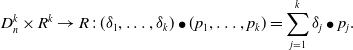 \begin{equation*} D_n^k \times R^k \rightarrow R \,:\, (\delta_1,\ldots,\delta_k) \bullet (p_1,\ldots,p_k)= \sum_{j=1}^k \delta_j \bullet p_j. \end{equation*}
Fix a submodule M of
 $R^k$
and let
$R^k$
and let
 $P_1,\ldots,P_s$
be its associated primes, as in Section 3. A differential primary decomposition of M is a list
$P_1,\ldots,P_s$
be its associated primes, as in Section 3. A differential primary decomposition of M is a list
 $\mathcal{A}_1,\ldots,\mathcal{A}_s$
of finite subsets of
$\mathcal{A}_1,\ldots,\mathcal{A}_s$
of finite subsets of
 $D_n^k$
such that
$D_n^k$
such that
 \begin{equation}M = \bigl\{ m \in R^k \,:\, \delta \bullet m \in P_i\ \ \hbox{for all}\ \delta \in \mathcal{A}_i\ \hbox{and}\ i=1,2, \ldots,s \bigr\}.\end{equation}
This is a membership test for the module M using differential operators. This test is geometric since the polynomial
 $\delta \bullet m $
lies in
$\delta \bullet m $
lies in
 $P_i $
if and only if it vanishes on the variety
$P_i $
if and only if it vanishes on the variety
 $V_i=V(P_i)$
.
$V_i=V(P_i)$
.
Theorem 4.1 Every submodule M of
 $R^k$
has a differential primary decomposition. We can choose the sets
$R^k$
has a differential primary decomposition. We can choose the sets
 $\mathcal{A}_1,\ldots,\mathcal{A}_s$
such that
$\mathcal{A}_1,\ldots,\mathcal{A}_s$
such that
 $|\mathcal{A}_i|$
is the arithmetic length of M along the prime
$|\mathcal{A}_i|$
is the arithmetic length of M along the prime
 $P_i$
.
$P_i$
.
Proof and discussion. The result is proved in [Reference Cid-Ruiz and Sturmfels12] and further refined in [Reference Chen and Cid-Ruiz9]. These sources also develop an algorithm. We shall explain this in Section 5, along with a discussion of the Macaulay2 command solvePDE, which computes differential primary decompositions.
![]()
The differential operators in
 $\mathcal{A}_1,\ldots,\mathcal{A}_s$
are known as Noetherian operators in the literature; see [Reference Chen, Härkönen, Krone and Leykin10, Reference Cid-Ruiz, Homs and Sturmfels11, Reference Damiano, Sabadini and Struppa15, Reference Oberst31]. Theorem 4.1 says that we can find a collection of
$\mathcal{A}_1,\ldots,\mathcal{A}_s$
are known as Noetherian operators in the literature; see [Reference Chen, Härkönen, Krone and Leykin10, Reference Cid-Ruiz, Homs and Sturmfels11, Reference Damiano, Sabadini and Struppa15, Reference Oberst31]. Theorem 4.1 says that we can find a collection of
 $\textrm{amult}(M) = m_1 + \cdots + m_s$
Noetherian operators in
$\textrm{amult}(M) = m_1 + \cdots + m_s$
Noetherian operators in
 $D_n^k$
to characterize membership in the module M.
$D_n^k$
to characterize membership in the module M.
Remark 4.2 The construction of Noetherian operators is studied in [Reference Björk7, Reference Chen, Cid-Ruiz, Härkönen, Krone and Leykin8, Reference Chen, Härkönen, Krone and Leykin10, Reference Cid-Ruiz, Homs and Sturmfels11, Reference Hörmander23, Reference Oberst31]. Some of these sources offer explicit methods, while others remain at an abstract level. All previous methods share one serious shortcoming, namely they yield operators separately for each primary component
 $M_i$
of M. They do not take into account how one primary component is embedded into another. This leads to a number of operators that can be much larger than amult (M). We refer to [Reference Cid-Ruiz and Sturmfels12, Example 5.6] for an instance from algebraic statistics where the previous methods require 1044 Noetherian operators, while
$M_i$
of M. They do not take into account how one primary component is embedded into another. This leads to a number of operators that can be much larger than amult (M). We refer to [Reference Cid-Ruiz and Sturmfels12, Example 5.6] for an instance from algebraic statistics where the previous methods require 1044 Noetherian operators, while
 ${\textrm{amult}}(M) = 207$
suffice.
${\textrm{amult}}(M) = 207$
suffice.
While Theorem 4.1 makes no claim of minimality, it is known that
 $\textrm{amult}(M)$
is the minimal number of Noetherian operators required for a differential primary decomposition of a certain desirable form. To make this precise, we begin with a few necessary definitions. For any given subset
$\textrm{amult}(M)$
is the minimal number of Noetherian operators required for a differential primary decomposition of a certain desirable form. To make this precise, we begin with a few necessary definitions. For any given subset
 $\mathcal{S}$
of
$\mathcal{S}$
of
 $\{x_1,\ldots,x_n\}$
, the relative Weyl algebra is defined as the subring of the Weyl algebra
$\{x_1,\ldots,x_n\}$
, the relative Weyl algebra is defined as the subring of the Weyl algebra
 $D_n$
using only differential operators corresponding to variables not in
$D_n$
using only differential operators corresponding to variables not in
 $\mathcal{S}$
:
$\mathcal{S}$
:
 \begin{equation} D_n(\mathcal{S}) \,:\!=\, R \langle \partial_{x_i} \,:\, x_i \not \in \mathcal{S} \rangle \subseteq D_n.\end{equation}
Thus, if
 $\mathcal{S} = \emptyset$
, then
$\mathcal{S} = \emptyset$
, then
 $D_n(\mathcal{S}) = D_n$
, and if
$D_n(\mathcal{S}) = D_n$
, and if
 $\mathcal{S} = \{x_1,\ldots,x_n\}$
, then
$\mathcal{S} = \{x_1,\ldots,x_n\}$
, then
 $D_n(\mathcal{S}) = R= K[x_1,\ldots,x_n]$
.
$D_n(\mathcal{S}) = R= K[x_1,\ldots,x_n]$
.
For any prime ideal
 $P_i$
in R we fix a set
$P_i$
in R we fix a set
 $\mathcal{S}_i \subseteq \{x_1,\ldots,x_n\}$
that satisfies
$\mathcal{S}_i \subseteq \{x_1,\ldots,x_n\}$
that satisfies
 $K[\mathcal{S}_i] \cap P_i = \{0\}$
and is maximal with this property. Thus,
$K[\mathcal{S}_i] \cap P_i = \{0\}$
and is maximal with this property. Thus,
 $\mathcal{S}_i$
is a maximal independent set of coordinates on the irreducible variety
$\mathcal{S}_i$
is a maximal independent set of coordinates on the irreducible variety
 $V(P_i)$
. Equivalently,
$V(P_i)$
. Equivalently,
 $\mathcal{S}_i$
is a basis of the algebraic matroid defined by the prime
$\mathcal{S}_i$
is a basis of the algebraic matroid defined by the prime
 $P_i$
; cf. [Reference Michałek and Sturmfels27, Example 13.2]. The cardinality of
$P_i$
; cf. [Reference Michałek and Sturmfels27, Example 13.2]. The cardinality of
 $\mathcal{S}_i$
equals the dimension of
$\mathcal{S}_i$
equals the dimension of
 $V(P_i)$
.
$V(P_i)$
.
Theorem 4.3 The differential primary decomposition in Theorem 4.1 can be chosen so that
 $\mathcal{A}_i \subset D_n(\mathcal{S}_i)^k$
. The arithmetic length of M along
$\mathcal{A}_i \subset D_n(\mathcal{S}_i)^k$
. The arithmetic length of M along
 $P_i$
is a lower bound for the cardinality of
$P_i$
is a lower bound for the cardinality of
 $\mathcal{A}_i$
in any differential primary decomposition of M such that
$\mathcal{A}_i$
in any differential primary decomposition of M such that
 $\mathcal{A}_i \subset D_n(\mathcal{S}_i)^k$
for
$\mathcal{A}_i \subset D_n(\mathcal{S}_i)^k$
for
 $i = 1,\ldots,s$
.
$i = 1,\ldots,s$
.
Proof and discussion. This was shown in [Reference Cid-Ruiz and Sturmfels12, Theorem 4.6]. The case of ideals
 $(k=1)$
appears in [Reference Cid-Ruiz and Sturmfels12, Theorem 3.6]. See also [Reference Chen and Cid-Ruiz9]. The theory developed in [Reference Cid-Ruiz and Sturmfels12] is more general in that R can be any Noetherian K-algebra. In this paper, we restrict to polynomial rings
$(k=1)$
appears in [Reference Cid-Ruiz and Sturmfels12, Theorem 3.6]. See also [Reference Chen and Cid-Ruiz9]. The theory developed in [Reference Cid-Ruiz and Sturmfels12] is more general in that R can be any Noetherian K-algebra. In this paper, we restrict to polynomial rings
 $R = K[x_1,\ldots,x_n]$
where K is a subfield of
$R = K[x_1,\ldots,x_n]$
where K is a subfield of
 $\mathbb{C}$
. That case is treated in detail in [Reference Chen and Cid-Ruiz9].
$\mathbb{C}$
. That case is treated in detail in [Reference Chen and Cid-Ruiz9].
![]()
We next argue that Theorems 2.2 and 4.1 are really two sides of the same coin. Every element A in the Weyl algebra
 $D_n$
acts as a differential operator with polynomial coefficients on functions in the unknowns
$D_n$
acts as a differential operator with polynomial coefficients on functions in the unknowns
 ${\bf x} = (x_1,\ldots,x_n)$
. Such a differential operator has a unique representation where all derivatives are moved to the right of the polynomial coefficients:
${\bf x} = (x_1,\ldots,x_n)$
. Such a differential operator has a unique representation where all derivatives are moved to the right of the polynomial coefficients:
 \begin{equation}\qquad A({\bf x},\partial_{\bf x}) = \sum_{{\bf r},{\bf s} \in \mathbb{N}^n} c_{{\bf r},{\bf s}} x_1^{r_1} \cdots x_n^{r_n} \partial_{x_1}^{s_1} \cdots \partial_{x_n}^{s_n} , \qquad{\textrm{where}} c_{{\bf r},{\bf s}} \in K .\end{equation}
There is a natural K-linear isomorphism between the Weyl algebra
 $D_n$
and the polynomial ring
$D_n$
and the polynomial ring
 $K[{\bf x},{\bf z}]$
which takes the operator A in (4.3) to the following polynomial B in 2n variables:
$K[{\bf x},{\bf z}]$
which takes the operator A in (4.3) to the following polynomial B in 2n variables:
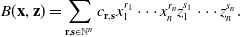 \begin{equation} B({\bf x},{\bf z}) = \sum_{{\bf r},{\bf s} \in \mathbb{N}^n} c_{{\bf r},{\bf s}} x_1^{r_1} \cdots x_n^{r_n} z_1^{s_1} \cdots z_n^{s_n} . \qquad \qquad \quad \end{equation}
In Sections 1, 2, and 3, polynomials in
 $R = K[x_1,\ldots,x_n] = K[\partial_1,\ldots,\partial_n] $
act as differential operators on functions in the unknowns
$R = K[x_1,\ldots,x_n] = K[\partial_1,\ldots,\partial_n] $
act as differential operators on functions in the unknowns
 ${\bf z} = (z_1,\ldots,z_n)$
. For such operators, polynomials in x are constants. By contrast, in the current section, we introduced the Weyl algebra
${\bf z} = (z_1,\ldots,z_n)$
. For such operators, polynomials in x are constants. By contrast, in the current section, we introduced the Weyl algebra
 $D_n$
. Its elements act on functions in
$D_n$
. Its elements act on functions in
 ${\bf x} = (x_1,\ldots,x_n)$
, with polynomials in z being constants. These two different actions of differential operators, by
${\bf x} = (x_1,\ldots,x_n)$
, with polynomials in z being constants. These two different actions of differential operators, by
 $D_n$
and R on scalar-valued functions, extend to actions by
$D_n$
and R on scalar-valued functions, extend to actions by
 $D_n^k$
and
$D_n^k$
and
 $R^k$
on vector-valued functions. We highlight the following key point:
$R^k$
on vector-valued functions. We highlight the following key point:
 \begin{equation} {Our\, distinction\, between\, the\, {z} -variables\, and\, {x}-variables\, is \, absolutely\, essential.}\end{equation}
The following theorem is the punchline of this section. It allows us to identify Noetherian operators (4.3) with Noetherian multipliers (4.4). This was assumed tacitly in [Reference Cid-Ruiz, Homs and Sturmfels11, Section 3].
Theorem 4.4 Consider any differential primary decomposition of the module M as in Theorem 4.3. Then this translates into an Ehrenpreis–Palamodov representation of the solution space
 ${\textrm{Sol}}(M)$
. Namely, if we replace each operator
${\textrm{Sol}}(M)$
. Namely, if we replace each operator
 $A({\bf x},\partial_{\bf x})$
in
$A({\bf x},\partial_{\bf x})$
in
 $\mathcal{A}_i$
by the corresponding polynomial
$\mathcal{A}_i$
by the corresponding polynomial
 $B({\bf x},{\bf z})$
, then these
$B({\bf x},{\bf z})$
, then these
 ${\textrm{amult}}(M)$
polynomials satisfy the conclusion of Theorem 2.2.
${\textrm{amult}}(M)$
polynomials satisfy the conclusion of Theorem 2.2.
Example 4.5 (
 $k=l=n=1$
) We illustrate Theorem 4.4 and the warning (4.5) for an ODE (1.1) with
$k=l=n=1$
) We illustrate Theorem 4.4 and the warning (4.5) for an ODE (1.1) with
 $m=3$
. Set
$m=3$
. Set
 $ p(x) = x^3 + 3 x^2 - 9x + 5 = (x-1)^2 (x+5)$
in (1.3). The ideal
$ p(x) = x^3 + 3 x^2 - 9x + 5 = (x-1)^2 (x+5)$
in (1.3). The ideal
 $I = \langle p \rangle$
has
$I = \langle p \rangle$
has
 $s=2$
associated primes in
$s=2$
associated primes in
 $R = \mathbb{Q}[x] $
, namely
$R = \mathbb{Q}[x] $
, namely
 $P_1 = \langle x-1 \rangle $
and
$P_1 = \langle x-1 \rangle $
and
 $P_2 = \langle x+5 \rangle$
, with
$P_2 = \langle x+5 \rangle$
, with
 $m_1 = 2$
and
$m_1 = 2$
and
 $m_2=1$
, so
$m_2=1$
, so
 ${\textrm{amult}}(I) = 3$
. A differential primary decomposition of I is given by
${\textrm{amult}}(I) = 3$
. A differential primary decomposition of I is given by
 $\mathcal{A}_1 = \{1,\partial_x \}$
and
$\mathcal{A}_1 = \{1,\partial_x \}$
and
 $\mathcal{A}_2 = \{1\}$
. The three Noetherian operators translate into the Noetherian multipliers
$\mathcal{A}_2 = \{1\}$
. The three Noetherian operators translate into the Noetherian multipliers
 $B_{11} = 1, B_{12} = z, B_{21} = 1$
. The integrals in (2.6) now furnish the general solution
$B_{11} = 1, B_{12} = z, B_{21} = 1$
. The integrals in (2.6) now furnish the general solution
 $ \phi(z) = \alpha {\textrm{exp}}(z) + \beta z {\textrm{exp}}(z) + \gamma {\textrm{exp}}({-}5z) $
to the differential equation
$ \phi(z) = \alpha {\textrm{exp}}(z) + \beta z {\textrm{exp}}(z) + \gamma {\textrm{exp}}({-}5z) $
to the differential equation
 $\phi''' + 3 \phi'' - 9 \phi' + 5 \phi = 0$
.
$\phi''' + 3 \phi'' - 9 \phi' + 5 \phi = 0$
.
The derivation of Theorem 4.4 rests on the following lemma on duality between x and z.
Lemma 4.6 Let p and q be polynomials in n unknowns with coefficients in K. We have
 \begin{equation} q(\partial_{\bf z}) \bullet \bigl(p({\bf z}) \exp({\bf x}^t {\bf z}) \bigr) = p(\partial_{\bf x}) \bullet \bigl( q({\bf x}) \exp({\bf x}^t {\bf z}) \bigr).\end{equation}
Proof. The parenthesized expression on the left equals
 $p(\partial_{\bf x}) \bullet {\textrm{exp}}({\bf x}^t {\bf z})$
, while that on the right equals
$p(\partial_{\bf x}) \bullet {\textrm{exp}}({\bf x}^t {\bf z})$
, while that on the right equals
 $q(\partial_{\bf z}) \bullet {\textrm{exp}}({\bf x}^t {\bf z})$
. Therefore, the expression in (4.6) is the result of applying the operator
$q(\partial_{\bf z}) \bullet {\textrm{exp}}({\bf x}^t {\bf z})$
. Therefore, the expression in (4.6) is the result of applying the operator
 $p(\partial_{\bf x}) q(\partial_{\bf z}) = q(\partial_{\bf z}) p(\partial_{\bf x}) $
to
$p(\partial_{\bf x}) q(\partial_{\bf z}) = q(\partial_{\bf z}) p(\partial_{\bf x}) $
to
 $ \exp({\bf x}^t {\bf z}) $
, when viewed as a function in 2n unknowns.
$ \exp({\bf x}^t {\bf z}) $
, when viewed as a function in 2n unknowns.
![]()
We now generalize this lemma to
 $k \geq 2$
, we replace p by a polynomial vector that depends on both x and z, and we rename that vector using the identification between (4.3) and (4.4).
$k \geq 2$
, we replace p by a polynomial vector that depends on both x and z, and we rename that vector using the identification between (4.3) and (4.4).
Proposition 4.7 Let
 $B({\bf x},{\bf z})$
be a k-tuple of polynomials in 2n variables and
$B({\bf x},{\bf z})$
be a k-tuple of polynomials in 2n variables and
 $A({\bf x},\partial_{\bf x}) \in D_n^k$
the corresponding k-tuple of differential operators in the Weyl algebra. Then we have
$A({\bf x},\partial_{\bf x}) \in D_n^k$
the corresponding k-tuple of differential operators in the Weyl algebra. Then we have
 \begin{align} q(\partial_\mathbf{z}) \bullet (B(\mathbf{x}, \mathbf{z}) \exp(\mathbf{x}^t \mathbf{z})) = A(\mathbf{x}, \partial_\mathbf{x}) \bullet (q(\mathbf{x}) \exp(\mathbf{x}^t \mathbf{z})) . \end{align}
Proof. If
 $k=1$
, we write
$k=1$
, we write
 $A(\mathbf{x}, \partial_\mathbf{x}) = \sum_{\alpha} c_\alpha(\mathbf{x}) \partial_\mathbf{x}^\alpha$
as in (4.3) and
$A(\mathbf{x}, \partial_\mathbf{x}) = \sum_{\alpha} c_\alpha(\mathbf{x}) \partial_\mathbf{x}^\alpha$
as in (4.3) and
 $B({\bf x},{\bf z}) = \sum_{\alpha} c_\alpha(\mathbf{x}) \mathbf{z}^\alpha$
as in (4.4). Only finitely many of the polynomials
$B({\bf x},{\bf z}) = \sum_{\alpha} c_\alpha(\mathbf{x}) \mathbf{z}^\alpha$
as in (4.4). Only finitely many of the polynomials
 $c_\alpha(\mathbf{x})$
are nonzero. Applying Lemma 4.6 gives
$c_\alpha(\mathbf{x})$
are nonzero. Applying Lemma 4.6 gives
 \begin{equation*} \begin{matrix} A(\mathbf{x}, \partial_\mathbf{x}) \bullet (q(\mathbf{x}) \exp(\mathbf{x}^t \mathbf{z})) = \sum_\alpha c_\alpha(\mathbf{x}) q(\partial_\mathbf{z}) \bullet ({\bf z}^\alpha \exp(\mathbf{x}^t \mathbf{z})) = q(\partial_\mathbf{z}) \bullet (B(\mathbf{x}, \mathbf{z}) \exp(\mathbf{x}^t \mathbf{z})). \end{matrix}\end{equation*}
The extension from
 $k=1$
to
$k=1$
to
 $k \geq 2$
follows because the differential operation
$k \geq 2$
follows because the differential operation
 $\bullet$
is K-linear.
$\bullet$
is K-linear.
![]()
We now take a step toward proving Theorem 4.4 in the case
 $s=1$
. Let M be a primary submodule of
$s=1$
. Let M be a primary submodule of
 $R^k$
with
$R^k$
with
 $\textrm{Ass}(M) = \{P\}$
. Its support
$\textrm{Ass}(M) = \{P\}$
. Its support
 $V(M) = V(P)$
is an irreducible affine variety in
$V(M) = V(P)$
is an irreducible affine variety in
 $\mathbb{C}^n$
. Consider the sets of all Noetherian operators and all Noetherian multipliers:
$\mathbb{C}^n$
. Consider the sets of all Noetherian operators and all Noetherian multipliers:
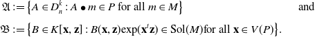 \begin{align} \mathfrak{A} & \,:\!= \bigl\{ A \in D_n^k\,:\, A \bullet m \in P\ \hbox{for all}\ m \in M \bigr\} \qquad \qquad \qquad \qquad \qquad {\textrm{and}} \nonumber\\[4pt] \mathfrak{B} & \,:\!= \bigl\{B \in K[{\bf x},{\bf z}]\,:\, B({\bf x},{\bf z}) {\textrm{exp}}({\bf x}^t {\bf z}) \in {\textrm{Sol}}(M)\hbox{for all ${\bf x} \in V(P) $} \bigr\}.\end{align}
Proposition 4.8 The bijection between
 $D_n^k$
and
$D_n^k$
and
 $K[{\bf x},{\bf z}]^k$
, given by identifying the operator A in (4.3) with the polynomial B in (4.4), restricts to a bijection between the sets
$K[{\bf x},{\bf z}]^k$
, given by identifying the operator A in (4.3) with the polynomial B in (4.4), restricts to a bijection between the sets
 $\mathfrak{A}$
and
$\mathfrak{A}$
and
 $\mathfrak{B}$
.
$\mathfrak{B}$
.
Proof. Let
 $m_1,\ldots,m_l \in K[{\bf x}]^k$
be generators of M. Suppose
$m_1,\ldots,m_l \in K[{\bf x}]^k$
be generators of M. Suppose
 $A \in \mathfrak{A}$
. Then
$A \in \mathfrak{A}$
. Then
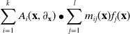 \begin{align*} \sum_{i = 1}^k A_i(\mathbf{x}, \partial_\mathbf{x}) \bullet \sum_{j = 1}^l m_{ij}(\mathbf{x}) f_j(\mathbf{x}) \end{align*}
vanishes for all
 $\mathbf{x} \in V(P)$
and all polynomials
$\mathbf{x} \in V(P)$
and all polynomials
 $f_1,\ldots,f_l \in \mathbb{C}[\mathbf{x}]$
. Since the space of complex-valued polynomials is dense in the space of all entire functions on
$f_1,\ldots,f_l \in \mathbb{C}[\mathbf{x}]$
. Since the space of complex-valued polynomials is dense in the space of all entire functions on
 $\mathbb{C}^n$
, the preceding implies
$\mathbb{C}^n$
, the preceding implies
 \begin{equation*} \sum_{i = 1}^k A_i(\mathbf{x}, \partial_\mathbf{x}) \bullet m_{ij}(\mathbf{x}) \exp(\mathbf{x}^t\mathbf{z}) = 0 \quad \hbox{for all $\mathbf{z} \in \mathbb{C}^n$, $\mathbf{x} \in V(P)$ and $j = 1,\ldots,l$.}\end{equation*}
Using Proposition 4.7, this yields
 \begin{equation*} \sum_{i = 1}^k m_{ij}(\partial_\mathbf{z}) \bullet B_i(\mathbf{x}, \mathbf{z}) \exp(\mathbf{x}^t\mathbf{z})= 0 \quad \hbox{for all $\mathbf{z} \in \mathbb{C}^n$, $\mathbf{x} \in V(P)$ and $j = 1,\ldots,l$.} \end{equation*}
We conclude that the polynomial vector
 $B(\mathbf{x},\mathbf{z}) $
corresponding to
$B(\mathbf{x},\mathbf{z}) $
corresponding to
 $A({\bf x},\partial_{\bf x})$
lies in
$A({\bf x},\partial_{\bf x})$
lies in
 $\mathfrak{B}$
.
$\mathfrak{B}$
.
To prove the converse, we note that the implications above are reversible. Thus, if
 $B({\bf x},{\bf z}) $
is in
$B({\bf x},{\bf z}) $
is in
 $\mathfrak{B}$
, then
$\mathfrak{B}$
, then
 $A({\bf x},\partial_{\bf x})$
is in
$A({\bf x},\partial_{\bf x})$
is in
 $\mathfrak{A}$
. This uses the fact that linear combinations of the exponential functions
$\mathfrak{A}$
. This uses the fact that linear combinations of the exponential functions
 $\mathbf{x} \to \exp(\mathbf{x}^t \mathbf{z})$
, for
$\mathbf{x} \to \exp(\mathbf{x}^t \mathbf{z})$
, for
 ${\bf z} \in \mathbb{C}^n$
, are also dense in the space of entire functions.
${\bf z} \in \mathbb{C}^n$
, are also dense in the space of entire functions.
![]()
Proof of Theorem 4.4. Let
 $\mathcal{A}$
be any finite subset of
$\mathcal{A}$
be any finite subset of
 $\mathfrak{A}$
which gives a differential primary decomposition of the P-primary module M. This exists and can be chosen to have cardinality equal to the length of M along P. Let
$\mathfrak{A}$
which gives a differential primary decomposition of the P-primary module M. This exists and can be chosen to have cardinality equal to the length of M along P. Let
 $\mathcal{B}$
be the set of Noetherian multipliers (4.4) corresponding to the set
$\mathcal{B}$
be the set of Noetherian multipliers (4.4) corresponding to the set
 $\mathcal{A}$
of Noetherian operators (4.3). Proposition 4.8 shows that the exponential function
$\mathcal{A}$
of Noetherian operators (4.3). Proposition 4.8 shows that the exponential function
 ${\bf z} \to B({\bf x},{\bf z}) {\textrm{exp}}({\bf x}^t {\bf z})$
is in
${\bf z} \to B({\bf x},{\bf z}) {\textrm{exp}}({\bf x}^t {\bf z})$
is in
 ${\textrm{Sol}}(M)$
whenever
${\textrm{Sol}}(M)$
whenever
 ${\bf x} \in V(P)$
and
${\bf x} \in V(P)$
and
 $B \in \mathcal{B}$
. Hence all
$B \in \mathcal{B}$
. Hence all
 $\mathbb{C}$
-linear combinations of such functions are in
$\mathbb{C}$
-linear combinations of such functions are in
 ${\textrm{Sol}}(M)$
. More generally, by differentiating under the integral sign, we find that all functions of the following form are solutions of M:
${\textrm{Sol}}(M)$
. More generally, by differentiating under the integral sign, we find that all functions of the following form are solutions of M:
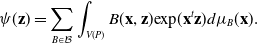 \begin{equation*} \psi({\bf z}) = \sum_{B \in \mathcal{B}} \int_{V(P)} B({\bf x},{\bf z}) {\textrm{exp}}({\bf x}^t {\bf z}) d\mu_B({\bf x}).\end{equation*}
We need to argue that all solutions in
 $\mathcal{F} = C^\infty(\Omega)$
admit such an integral representation. Suppose first that all associated primes of M are minimal. Then each
$\mathcal{F} = C^\infty(\Omega)$
admit such an integral representation. Suppose first that all associated primes of M are minimal. Then each
 $\mathcal{A}_i$
spans a bimodule in the sense of [Reference Chen and Cid-Ruiz9, Theorem 3.2 (d)]. Hence, for each associated prime
$\mathcal{A}_i$
spans a bimodule in the sense of [Reference Chen and Cid-Ruiz9, Theorem 3.2 (d)]. Hence, for each associated prime
 $P_i$
, the module
$P_i$
, the module
 \begin{align*} M_i = \{ m \in R^k \,:\, \delta \bullet m \in P_i \text{ for all } \delta \in \mathcal{A}_i \}\end{align*}
is
 $P_i$
-primary, and
$P_i$
-primary, and
 $M = M_1 \cap \dotsb \cap M_s$
is a minimal primary decomposition. The operators in
$M = M_1 \cap \dotsb \cap M_s$
is a minimal primary decomposition. The operators in
 $\mathcal{A}_i$
are in the relative Weyl algebra
$\mathcal{A}_i$
are in the relative Weyl algebra
 $D_n(\mathcal{S}_i)$
and fully characterize the
$D_n(\mathcal{S}_i)$
and fully characterize the
 $P_i$
-primary component of M. We may thus follow the classical analytical constructions in the books [Reference Björk7, Reference Hörmander23, Reference Palamodov32] to patch together the integral representation of
$P_i$
-primary component of M. We may thus follow the classical analytical constructions in the books [Reference Björk7, Reference Hörmander23, Reference Palamodov32] to patch together the integral representation of
 ${\textrm{Sol}}(M_i)$
for
${\textrm{Sol}}(M_i)$
for
 $i=1,\ldots,s$
, under the correspondence of Noetherian operators and Noetherian multipliers. Therefore, all solutions have the form (2.6).
$i=1,\ldots,s$
, under the correspondence of Noetherian operators and Noetherian multipliers. Therefore, all solutions have the form (2.6).
Things are more delicate when M has embedded primes. Namely, if
 $P_i$
is embedded, then the operators in
$P_i$
is embedded, then the operators in
 $\mathcal{A}_i$
only characterize the contribution of the
$\mathcal{A}_i$
only characterize the contribution of the
 $P_i$
-primary component relative to all other components contained in
$P_i$
-primary component relative to all other components contained in
 $P_i$
. We see this in Section 5. One argues by enlarging
$P_i$
. We see this in Section 5. One argues by enlarging
 $\mathcal{A}_i$
to vector space generators of the relevant bimodule. Then the previous patching argument applies. And, afterward one shows that the added summand in the integral representation are redundant because they are covered by associated varieties
$\mathcal{A}_i$
to vector space generators of the relevant bimodule. Then the previous patching argument applies. And, afterward one shows that the added summand in the integral representation are redundant because they are covered by associated varieties
 $V(P_j)$
containing
$V(P_j)$
containing
 $V(P_i)$
.
$V(P_i)$
.
![]()
5. Software and algorithm
In this section, we present an algorithm for solving linear PDE with constant coefficients. It is based on the methods for ideals given in [Reference Chen, Cid-Ruiz, Härkönen, Krone and Leykin8, Reference Chen, Härkönen, Krone and Leykin10, Reference Cid-Ruiz, Homs and Sturmfels11]. The case of modules appears in [Reference Chen and Cid-Ruiz9]. We note that the computation of Noetherian operators has a long history, going back to work in the 1990’s by Ulrich Oberst [Reference Oberst28, Reference Oberst29, Reference Oberst30, Reference Oberst31], who developed a construction of Noetherian operators for primary modules. This was further developed by Damiano, Sabadini and Struppa [Reference Damiano, Sabadini and Struppa15] who presented the first Gröbner-based algorithm. It works for primary ideals under the restrictive assumption that the characteristic variety has a rational point after passing to a (algebraically nonclosed) field of fractions. Their article also points to an implementation in CoCoA, but we were unable to access that code. Since these early approaches rely on the ideals or modules being primary, using them in practice requires first computing a primary decomposition. If there are embedded primes, the number of Noetherian operators output by these methods will not be minimal either.
We here present a new algorithm that is universally applicable, to all ideals and modules over a polynomial ring. There are no restrictions on the input and the output is minimal. The input is a submodule M of
 $R^k$
, where
$R^k$
, where
 $R = K[x_1,\ldots,x_n]$
. The output is a differential primary decomposition of size
$R = K[x_1,\ldots,x_n]$
. The output is a differential primary decomposition of size
 ${\textrm{amult}}(M)$
as in Theorem 4.3. A first step is to find
${\textrm{amult}}(M)$
as in Theorem 4.3. A first step is to find
 ${\textrm{Ass}}(M) = \{P_1,\ldots,P_s\}$
. For each associated prime
${\textrm{Ass}}(M) = \{P_1,\ldots,P_s\}$
. For each associated prime
 $P_i$
, the elements
$P_i$
, the elements
 $A({\bf x},\partial_{\bf x})$
in the finite set
$A({\bf x},\partial_{\bf x})$
in the finite set
 $\mathcal{A}_i \subset D_n(\mathcal{S}_i)$
are rewritten as polynomials
$\mathcal{A}_i \subset D_n(\mathcal{S}_i)$
are rewritten as polynomials
 $B({\bf x},{\bf z})$
, using the identification of (4.3) with (4.4). Only the
$B({\bf x},{\bf z})$
, using the identification of (4.3) with (4.4). Only the
 ${\textrm{codim}}(P_i)$
many variables
${\textrm{codim}}(P_i)$
many variables
 $z_i $
with
$z_i $
with
 $x_i \not\in \mathcal{S}_i$
appear in these Noetherian multipliers B.
$x_i \not\in \mathcal{S}_i$
appear in these Noetherian multipliers B.
We now describe our implementation for (2.7) in Macaulay2 [Reference Grayson and Stillman21]. The command is called solvePDE, as in [Reference Cid-Ruiz and Sturmfels12, Section 5]. It is distributed with Macaulay2 starting from version 1.18 in the package NoetherianOperators [Reference Chen, Cid-Ruiz, Härkönen, Krone and Leykin8]. The user begins by fixing a polynomial ring
 $R = K[x_1,\ldots,x_n]$
. Here K is usually the rational numbers
$R = K[x_1,\ldots,x_n]$
. Here K is usually the rational numbers
 $ \texttt{QQ}$
. Fairly arbitrary variable names
$ \texttt{QQ}$
. Fairly arbitrary variable names
 $x_i$
are allowed. The argument of solvePDE is an ideal in R or a submodule of
$x_i$
are allowed. The argument of solvePDE is an ideal in R or a submodule of
 $R^k$
. The output is a list of pairs
$R^k$
. The output is a list of pairs
 $\bigl\{P_i,\{B_{i1},\ldots,B_{i,m_i}\} \bigr\}$
for
$\bigl\{P_i,\{B_{i1},\ldots,B_{i,m_i}\} \bigr\}$
for
 $i=1,\ldots,s$
, where
$i=1,\ldots,s$
, where
 $P_i$
is a prime ideal given by generators in R, and each
$P_i$
is a prime ideal given by generators in R, and each
 $B_{ij}$
is a vector over a newly created polynomial ring
$B_{ij}$
is a vector over a newly created polynomial ring
 $K[x_1,\ldots,x_n,z_1,\ldots,z_n]$
. The new variables
$K[x_1,\ldots,x_n,z_1,\ldots,z_n]$
. The new variables
 $z_i$
are named internally by Macaulay2. The system writes
$z_i$
are named internally by Macaulay2. The system writes
 $ \texttt{d} x_i$
for
$ \texttt{d} x_i$
for
 $z_i$
. To be precise, each new variable is created from an old variable by prepending the character
$z_i$
. To be precise, each new variable is created from an old variable by prepending the character
 $ \texttt{d}$
. This notation can be confusing at first, but one gets used to it. The logic comes from the differential primary decompositions described in [Reference Cid-Ruiz and Sturmfels12, Section 5].
$ \texttt{d}$
. This notation can be confusing at first, but one gets used to it. The logic comes from the differential primary decompositions described in [Reference Cid-Ruiz and Sturmfels12, Section 5].
Each
 $B_{ij}$
in the output of solvePDE encodes an exponential solution
$B_{ij}$
in the output of solvePDE encodes an exponential solution
 $B_{ij}({\bf x},{\bf z}) {\textrm{exp}}({\bf x}^t {\bf z})$
to M. Here x are the old variables chosen by the user, and x denotes points in the irreducible variety
$B_{ij}({\bf x},{\bf z}) {\textrm{exp}}({\bf x}^t {\bf z})$
to M. Here x are the old variables chosen by the user, and x denotes points in the irreducible variety
 $V(P_i) \subseteq \mathbb{C}^n$
. The solution is a function in the new unknowns
$V(P_i) \subseteq \mathbb{C}^n$
. The solution is a function in the new unknowns
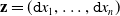 ${\bf z} = (\texttt{d}x_1,\ldots, \texttt{d}x_n)$
. For instance, if
${\bf z} = (\texttt{d}x_1,\ldots, \texttt{d}x_n)$
. For instance, if
 $n=3$
and the input is in the ring
$n=3$
and the input is in the ring
 $ \texttt{QQ[u,v,w]}$
, then the output lives in the ring
$ \texttt{QQ[u,v,w]}$
, then the output lives in the ring
 $ \texttt{QQ[u,v,w,du,dv,dw]}$
. Each solution to the PDE is a function
$ \texttt{QQ[u,v,w,du,dv,dw]}$
. Each solution to the PDE is a function
 $\psi(\texttt{du}, \texttt{dv}, \texttt{dw})$
, and these functions are parametrized by a variety
$\psi(\texttt{du}, \texttt{dv}, \texttt{dw})$
, and these functions are parametrized by a variety
 $V(P_i)$
in a 3-space whose coordinates are
$V(P_i)$
in a 3-space whose coordinates are
 $(\texttt{u}, \texttt{v}, \texttt{w})$
.
$(\texttt{u}, \texttt{v}, \texttt{w})$
.
We now demonstrate how this works for two examples featured in the introduction.
Example 5.1. Consider the third order ODE (1.1) in Example 4.5. We solve this as follows:
R = QQ[x]; I = ideal(x^3 + 3*x^2 - 9*x + 5); solvePDE(I)
{{ideal(x - 1), {| 1 |, | dx |}}, {ideal(x + 5), {| 1 |}}}
The first line is the input. The second line is the output created by solvePDE. This list of
 $s=2$
pairs encodes the general solution
$s=2$
pairs encodes the general solution
 $\phi(z)$
. Remember: z is the newly created symbol dx.
$\phi(z)$
. Remember: z is the newly created symbol dx.
Example 5.2. We solve the PDE (1.8) by typing the
 $ 2 \times 3$
matrix whose columns are (2.1):
$ 2 \times 3$
matrix whose columns are (2.1):
R = QQ[x1,x2,x3,x4];
M = image matrix {{x1^2,x2*x3,x1^2*x3},{x1*x2,x3^2,x1*x2*x4}}; solvePDE(M)
The reader is encouraged to run this code and to check that the output is the solution (1.9).
The method in solvePDE is described in Algorithm 1 below. A key ingredient is a translation map. We now explain this in the simplest case, when the module is supported in one point. Suppose
 $V(M) = \{\mathbf{u}\}$
for some
$V(M) = \{\mathbf{u}\}$
for some
 $\mathbf{u} \in K^n$
. We set
$\mathbf{u} \in K^n$
. We set
 $ \mathfrak{m}_\mathbf{u} = \langle x_1 - u_1, \ldots, x_n - u_n \rangle$
and
$ \mathfrak{m}_\mathbf{u} = \langle x_1 - u_1, \ldots, x_n - u_n \rangle$
and
 \begin{equation} \gamma_\mathbf{u} \,:\, R \to R , x_i \mapsto x_i + u_i \quad \text{ for } i=1,\ldots,n. \end{equation}
The following two results are straightforward. We will later use them when M is any primary module, u is the generic point of V(M), and
 $\mathbb{K} = K({\bf u})$
is the associated field extension of K.
$\mathbb{K} = K({\bf u})$
is the associated field extension of K.
Proposition 5.3 A constant coefficient operator
 $A(\partial_\mathbf{x})$
is a Noetherian operator for the
$A(\partial_\mathbf{x})$
is a Noetherian operator for the
 $\mathfrak{m}_\mathbf{u}$
-primary module M if and only if
$\mathfrak{m}_\mathbf{u}$
-primary module M if and only if
 $A(\partial_\mathbf{x})$
is a Noetherian operator for the
$A(\partial_\mathbf{x})$
is a Noetherian operator for the
 $\mathfrak{m}_0$
-primary module
$\mathfrak{m}_0$
-primary module
 $\hat M \,:\!=\, \gamma_\mathbf{u}(M)$
. Dually,
$\hat M \,:\!=\, \gamma_\mathbf{u}(M)$
. Dually,
 $B(\mathbf{z}) \exp(\mathbf{u}^t\mathbf{z}) $
is in
$B(\mathbf{z}) \exp(\mathbf{u}^t\mathbf{z}) $
is in
 $ \textrm{Sol}(M)$
if and only if
$ \textrm{Sol}(M)$
if and only if
 $B(\mathbf{z})$
is in
$B(\mathbf{z})$
is in
 $ \textrm{Sol}(\hat M)$
.
$ \textrm{Sol}(\hat M)$
.
We note that all Noetherian operators over a K-rational point can be taken to have constant coefficients. This follows from Theorem 3.8. This observation reduces the computation of solutions for a primary module to finding the polynomial solutions of the translated module. Next, we bound the degrees of these polynomials.
Proposition 5.4 Let
 $\hat M \subseteq R^k$
be an
$\hat M \subseteq R^k$
be an
 $\mathfrak{m}_0$
-primary module. There exists an integer r such that
$\mathfrak{m}_0$
-primary module. There exists an integer r such that
 $\mathfrak{m}_0^{r+1} R^k \subseteq \hat M$
. The space
$\mathfrak{m}_0^{r+1} R^k \subseteq \hat M$
. The space
 $\textrm{Sol}(\hat M)$
consists of k-tuples of polynomials of degree
$\textrm{Sol}(\hat M)$
consists of k-tuples of polynomials of degree
 $\leq r$
.
$\leq r$
.
Propositions 5.3 and 5.4 furnish a method for computing solutions of an
 $\mathfrak{m}_\mathbf{u}$
-primary module M. We start by translating M so that it becomes the
$\mathfrak{m}_\mathbf{u}$
-primary module M. We start by translating M so that it becomes the
 $\mathfrak{m}_0$
-primary module
$\mathfrak{m}_0$
-primary module
 $\hat M$
. The integer r provides an ansatz
$\hat M$
. The integer r provides an ansatz
 $ \sum_{j=1}^k\sum_{|\alpha| \leq r} v_{\alpha,j} \mathbf{z}^\alpha e_j $
for the polynomial solutions. The coefficients
$ \sum_{j=1}^k\sum_{|\alpha| \leq r} v_{\alpha,j} \mathbf{z}^\alpha e_j $
for the polynomial solutions. The coefficients
 $v_{\alpha,j}$
are computed by linear algebra over the ground field K. Here are the steps:
$v_{\alpha,j}$
are computed by linear algebra over the ground field K. Here are the steps:
-
1. Let r be the smallest integer such that
 $\mathfrak{m}_0^{r+1} R^k \subseteq \hat M$
.
$\mathfrak{m}_0^{r+1} R^k \subseteq \hat M$
. -
2. Let
$\textrm{Diff}( \hat M)$
be the matrix whose entries are the polynomials
$\hat m_i \bullet ({\bf z}^\alpha e_j) \in R$
. The row labels are the generators
$\hat m_1, \ldots, \hat m_l $
of
$\hat M$
, and the column labels are the
${\bf z}^\alpha e_j$
. -
3. Let
$\ker_K(\textrm{Diff}(\hat M))$
denote the K-linear subspace of the R-module
$\ker_R(\textrm{Diff}(\hat M))$
consisting of vectors
$(v_{\alpha,j}) $
with all entries in K. Every such vector gives a solution (5.2)
\begin{align} \sum_{j=1}^k \sum_{|\alpha| \leq r} v_{\alpha, j} {\bf z}^\alpha \exp(\mathbf{u}^t \mathbf{z}) e_j \in \textrm{Sol}(M).\end{align}


Example 5.5
 $[n=k=r=2]$
The following module is
$[n=k=r=2]$
The following module is
 $\mathfrak{m}_0$
-primary of multiplicity three:
$\mathfrak{m}_0$
-primary of multiplicity three:
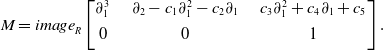 \begin{equation}M = {{image}}_R \begin{bmatrix}\partial_1^3 & \quad \partial_2 - c_1 \partial_1^2 - c_2 \partial_1 & \quad c_3 \partial_1^2 + c_4 \partial_1 + c_5 \\[4pt] 0 & \quad 0 & \quad 1 \\[4pt]\end{bmatrix}.\end{equation}
Here
 $c_1,c_2,c_3,c_4,c_5$
are arbitrary constants in K. The matrix
$c_1,c_2,c_3,c_4,c_5$
are arbitrary constants in K. The matrix
 ${\textrm{Diff}}(M)$
has three rows, one for each generator of M, and it has 12 columns, indexed by
${\textrm{Diff}}(M)$
has three rows, one for each generator of M, and it has 12 columns, indexed by
 $e_1,z_1e_1,\ldots , z_2^2 e_1,e_2,z_1e_2,\ldots , z_2^2 e_2$
. The space
$e_1,z_1e_1,\ldots , z_2^2 e_1,e_2,z_1e_2,\ldots , z_2^2 e_2$
. The space
 ${\textrm{ker}}_K({\textrm{Diff}}(M))$
is 3-dimensional. A basis furnishes the three polynomial solutions
${\textrm{ker}}_K({\textrm{Diff}}(M))$
is 3-dimensional. A basis furnishes the three polynomial solutions
 \begin{equation}\begin{bmatrix}-1 \\[4pt] c_5,\end{bmatrix} ,\begin{bmatrix} -(z_1+c_2 z_2) \\[4pt] c_5 z_1+c_2 c_5 z_2+c_4 \end{bmatrix} , \begin{bmatrix} -((z_1+c_2 z_2)^2 + 2 c_1 z_2) \\[4pt] c_5 (z_1{+}c_2 z_2)^2 + 2 c_4z_1 + 2 (c_1 c_5{+}c_2 c_4)z_2 + 2c_3 \end{bmatrix}.\end{equation}
We now turn to Algorithm 1. The input and output are as described in (2.7). The method was introduced in [Reference Chen and Cid-Ruiz9, Algorithm 4.6] for computing differential primary decompositions. We use it for solving PDE. It is implemented in Macaulay2 under the command solvePDE. In our discussion, the line numbers refer to the corresponding lines of pseudocode in Algorithm 1.
-
Line 1 We begin by finding all associated primes of M. These define the irreducible varieties
$V_i$
in (2.7). By [Reference Eisenbud, Huneke and Vasconcelos19, Theorem 1.1], the associated primes of codimension i coincide with the minimal primes of
$\textrm{Ann}\ \textrm{Ext}^i_R(M,R)$
. This reduces the problem of finding associated primes of a module to the more familiar problem of finding minimal primes of a polynomial ideal. This method is implemented and distributed with Macaulay2 starting from version 1.17 via the command associatedPrimes
$\texttt{R^k/M}$
. See [Reference Chen and Cid-Ruiz9, Section 2].


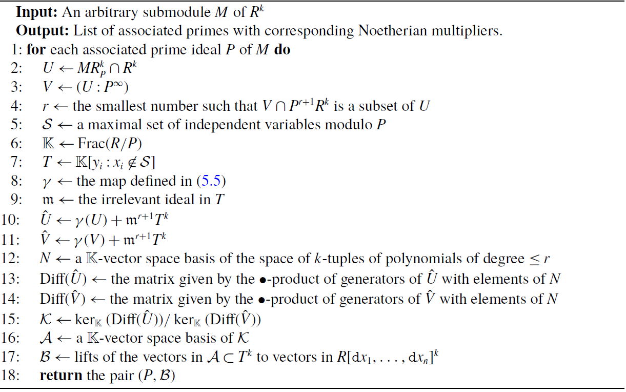
Algorithm 1 SolvePDE
The remaining steps are repeated for each
 $P \in \textrm{Ass}(M)$
. For a fixed associated prime P, our goal is to identify the contribution to
$P \in \textrm{Ass}(M)$
. For a fixed associated prime P, our goal is to identify the contribution to
 $\textrm{Sol}(M)$
of the P-primary component of M.
$\textrm{Sol}(M)$
of the P-primary component of M.
-
Lines 2–3 To achieve this goal, we study solutions for two different R-submodules of
$R^k$
. The first one, denoted U, is the intersection of all
$P_i$
-primary components of M, where
$P_i$
are the associated primes contained in P. Thus
$U = MR^k_P \cap R^k$
, which is the extension-contraction module of M under localization at P. It is computed as
$U = (M \,:\, f^\infty)$
, where
$f \in R$
is contained in every associated prime
$P_j$
not contained in P.The second module, denoted V, is the intersection of all
$P_i$
-primary components of M, where
$P_i$
is strictly contained in P. Hence,
$V = (U \,:\, P^\infty)$
is the saturation of U at P. We have
$U = V \cap Q$
, where Q is a P-primary component of M. Thus, the difference between the solution spaces
$\textrm{Sol}(U)$
and
$\textrm{Sol}(V)$
is caused by the primary module Q.When P is a minimal prime, U is the unique P-primary component of M, and
$V = R^k$
. Line 4 The integer r bounds the degree of Noetherian multipliers associated to U but not V. Namely, if the function
$\phi(\mathbf{z}) = B(\mathbf{x}, \mathbf{z}) \exp(\mathbf{x}^t \mathbf{z})$
lies in
$\textrm{Sol}(U) \backslash \textrm{Sol}(V)$
for all
$\mathbf{x} \in V(P)$
, then the
$\mathbf{z}$
-degree of the polynomial
$B(\mathbf{x}, \mathbf{z})$
is at most r. This will lead to an ansatz for the Noetherian multipliers responsible for the difference between
$\textrm{Sol}(U)$
and
$\textrm{Sol}(V)$
.Lines 5–8 The modules U and V are reduced to simpler modules
$\hat U$
and
$\hat V$
with similar properties. Namely,
$\hat U$
and
$\hat V$
are primary and their characteristic varieties are the origin. This reduction involves two new ingredients: a new polynomial ring T in fewer variables over a field
$\mathbb{K}$
that is a finite extension of K, and a ring map
$\gamma \,:\, R \to T$
.Fix a maximal set
$\mathcal{S} = \{x_{i_1},\ldots,x_{i_{n-c}}\}$
with
$P\cap K[x_{i_1},\ldots,x_{i_{n-c}}]=\{0\}$
. We define
$T\,:\!=\, \mathbb{K}[y_i\,:\, x_i\notin \mathcal{S}]$
, where
$\mathbb{K}=\textrm{Frac}(R/P)$
. This is a polynomial ring in
$n - |\mathcal{S}| = c$
new variables
$y_i$
, corresponding to the
$x_i$
not in the set
$\mathcal{S}$
of independent variables. Writing
$u_i$
for the image of
$x_i$
in
$\mathbb{K}=\textrm{Frac}(R/P)$
, the ring map
$\gamma$
is defined as follows: (5.5)By abuse of notation, we denote by
\begin{equation}\gamma \,:\, R \to T, \quad x_i\mapsto \begin{cases} y_i+u_i, & \text{ if } x_i\notin S,\\[4pt] \quad u_i, & \text{ if } x_i\in S. \end{cases} \end{equation}
$\gamma$
the extension of (5.5) to a map
$R^k \to T^k$
.
Lines 9–11 Let
$\mathfrak{m} \,:\!=\, \langle y_i \,:\, x_i \not \in \mathcal{S} \rangle $
be the irrelevant ideal of T. We define the T-submodules These modules are
\begin{equation*} \hat U \,:\!=\, \gamma(U) + \mathfrak{m}^{r+1} T^k \quad {\textrm{and}} \quad \hat V \,:\!=\, \gamma(U) + \mathfrak{m}^{r+1} T^k \quad {\textrm{of}}\ T^k. \end{equation*}
$\mathfrak{m}$
-primary: their solutions are finite-dimensional
$\mathbb{K}$
-vector spaces consisting of polynomials of degree
$\leq r$
. The polynomials in
$\textrm{Sol}(\hat U) \backslash \textrm{Sol}(\hat V)$
capture the difference between
$\hat U$
and
$\hat V$
, and also the difference between U and V after lifting.
-
Lines 12–14 We construct matrices
$\textrm{Diff}(\hat U)$
and
$\textrm{Diff}(\hat V)$
with entries in
$\mathbb{K} [z_i \,:\, x_i \not\in \mathcal{S}] $
. As in (5.2), their kernels over
$\mathbb{K}$
correspond to polynomial solutions of
$\hat U$
and
$\hat V$
. The set
$N = \{{\bf z}^\alpha e_j \,:\, |\alpha| \leq r, j=1,\ldots, k\}$
is a
$\mathbb{K}$
-basis for elements of degree
$\leq r$
in
$\mathbb{K}[z_i \,:\, x_i \not\in \mathcal{S}]^k$
. The
$y_i$
-variables act on the
$z_i$
variables as partial derivatives, i.e.
$y_i = \dfrac{\partial}{\partial z_i}$
. We define the matrix
$\textrm{Diff}(\hat U)$
as follows. Let
$\hat{U}_1,\ldots, \hat{U}_\ell$
be generators of
$\hat{U}$
. The rows of
$\textrm{Diff}(\hat{U})$
are indexed by these generators, the columns are indexed by N, and the entries are the polynomials
$\hat{U}_i\bullet {\bf z}^\alpha e_j$
. In the same way, we construct
$\textrm{Diff}(\hat{V})$
. -
Lines 15–16 Let
$\ker_\mathbb{K}(\textrm{Diff}(\hat U))$
be the space of vectors in the kernel of
$\textrm{Diff}(\hat U)$
whose entries are in
$\mathbb{K}$
. The
$\mathbb{K}$
-vector space
$\ker_\mathbb{K}(\textrm{Diff}(\hat U))$
parametrizes the polynomial solutions The same holds for
\begin{align*} \sum_{j=1}^k \sum_{|\alpha| \leq r} v_{\alpha,j} {\bf z}^\alpha e_j \in \textrm{Sol}(\hat U). \end{align*}
$\hat V$
. The quotient space
$\mathcal{K}\,:\!=\, \ker_\mathbb{K}(\textrm{Diff}(\hat U)) / \ker_\mathbb{K}(\textrm{Diff}(\hat V))$
characterizes excess solutions in
$\textrm{Sol}(\hat U)$
relative to
$\textrm{Sol}(\hat V)$
. Write
$\mathcal{A}$
for a
$\mathbb{K}$
-basis of
$\mathcal{K}$
.
-
Lines 17–18 We interpret
$\mathcal{A}$
as a set of Noetherian multipliers for M by performing a series of lifts and transformations. For each element
$\bar{\mathbf{v}} \in \mathcal{A}$
, we choose a representative
$\mathbf{v} \in \ker_\mathbb{K}(\textrm{Diff}(\hat U))$
. The entries of
$\mathbf{v}$
are in
$\mathbb{K} = \textrm{Frac}(R/P)$
and may contain denominators. Multiplying
$\mathbf{v}$
by a common multiple of the denominators yields a vector with entries in
$R/P$
, indexed by N. We lift this to a vector
$\mathbf{u} = (u_{\alpha,j})$
with entries in R. The Noetherian multiplier corresponding to u is the following vector in
$R[\texttt{d}x_i \,:\, x_i \not \in \mathcal{S}]^k$
: Applying the map
\begin{align*} B(\mathbf{x}, \mathbf{\texttt{d}x}) = \sum_{j=1}^k \sum_{|\alpha| \leq r} u_{\alpha,j}(\mathbf{x}) \mathbf{\texttt{d}x}^\alpha e_j . \end{align*}
$\bar{\mathbf{v}} \mapsto \mathbf{u}$
to each
$\bar{\mathbf{v}} \in \mathcal{A}$
yields a set
$\mathcal{B}$
of Noetherian multipliers. These multipliers describe the contribution of the P-primary component of M to
${\textrm{Sol}}(M)$
.


The output of Algorithm 1 is a list of pairs
 $(P, \mathcal{B})$
, where P ranges over
$(P, \mathcal{B})$
, where P ranges over
 ${\textrm{Ass}}(M)$
and
${\textrm{Ass}}(M)$
and
 $\mathcal{B} = \{B_1,\ldots,B_m\}$
is a subset of
$\mathcal{B} = \{B_1,\ldots,B_m\}$
is a subset of
 $R[\texttt{d}x_1, \ldots, \texttt{d}x_n]^k$
. The cardinality m is the multiplicity of M along P. The output describes the solutions to the PDE given by M. Consider the functions
$R[\texttt{d}x_1, \ldots, \texttt{d}x_n]^k$
. The cardinality m is the multiplicity of M along P. The output describes the solutions to the PDE given by M. Consider the functions
 \begin{equation*}\phi_P(\texttt{d}x_1,\ldots,\texttt{d}x_n)= \sum_{i=1}^m \int_{V(P)}B_i(\mathbf{x}, \mathbf{\texttt{d}x})\exp(x_1\texttt{d}x_1+\cdots+x_n\texttt{d}x_n){d\mu_i}(\mathbf{x}).\end{equation*}
Then the space of solutions to M consists of all functions
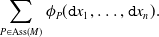 \begin{equation*}\sum_{P \in {\textrm{Ass}}(M)} \phi_P(\texttt{d}x_1,\ldots,\texttt{d}x_n).\end{equation*}
A differential primary decomposition of M is obtained from this by reading
 $\texttt{d}x_i$
as
$\texttt{d}x_i$
as
 $\partial_{x_i}$
. Indeed, the command differentialPrimaryDecomposition described in [Reference Chen and Cid-Ruiz9] is identical to our command solvePDE. All examples in [Reference Chen and Cid-Ruiz9, Section 6] can be interpreted as solving PDE.
$\partial_{x_i}$
. Indeed, the command differentialPrimaryDecomposition described in [Reference Chen and Cid-Ruiz9] is identical to our command solvePDE. All examples in [Reference Chen and Cid-Ruiz9, Section 6] can be interpreted as solving PDE.
6. Schemes and coherent sheaves
The concepts of schemes and coherent sheaves are central to modern algebraic geometry. These generalize varieties and vector bundles, and they encode geometric structures with multiplicities. The point is that the supports of coherent sheaves and other schemes are generally nonreduced. We here argue that our linear PDE offer a useful way to think about the geometry of these objects. That perspective motivated the writing of [Reference Michałek and Sturmfels27, Section 3.3].
The affine schemes we consider are defined by ideals I in a polynomial ring R. Likewise, submodules M of
 $R^k$
represent coherent sheaves on
$R^k$
represent coherent sheaves on
 $\mathbb{C}^n$
. We study the affine scheme
$\mathbb{C}^n$
. We study the affine scheme
 ${\textrm{Spec}}(R/I)$
and the coherent sheaf given by the module
${\textrm{Spec}}(R/I)$
and the coherent sheaf given by the module
 $R^k/M$
. The underlying geometric objects are the affine varieties V(I) and V(M) in
$R^k/M$
. The underlying geometric objects are the affine varieties V(I) and V(M) in
 $\mathbb{C}^n$
. The latter was discussed in Section 3. The solution spaces
$\mathbb{C}^n$
. The latter was discussed in Section 3. The solution spaces
 ${\textrm{Sol}}(I)$
or
${\textrm{Sol}}(I)$
or
 ${\textrm{Sol}}(M)$
furnish nonreduced structures on these varieties, encoded in the integral representations due to Ehrenpreis–Palamodov. According to Section 4, these are dual to differential primary decompositions. Coherent sheaves were a classical tool in the analysis of linear PDE, but in the analytic category, where their role was largely theoretical. The Ehrenpreis–Palamodov Fundamental Principle appears in Hörmander’s book under the header Coherent analytic sheaves on Stein manifolds [Reference Hörmander23, Chapter VII]. Likewise, Treves’ exposition, in the title of [Reference Treves35, Section 3.2], calls for Analytic sheaves to the rescue. By contrast, sheaves in this paper are concrete and algebraic: they are modules in Macaulay2.
${\textrm{Sol}}(M)$
furnish nonreduced structures on these varieties, encoded in the integral representations due to Ehrenpreis–Palamodov. According to Section 4, these are dual to differential primary decompositions. Coherent sheaves were a classical tool in the analysis of linear PDE, but in the analytic category, where their role was largely theoretical. The Ehrenpreis–Palamodov Fundamental Principle appears in Hörmander’s book under the header Coherent analytic sheaves on Stein manifolds [Reference Hörmander23, Chapter VII]. Likewise, Treves’ exposition, in the title of [Reference Treves35, Section 3.2], calls for Analytic sheaves to the rescue. By contrast, sheaves in this paper are concrete and algebraic: they are modules in Macaulay2.
One purpose of this section is to explore how PDE and their solutions behave under degenerations. We consider ideals and modules whose generators depend on a parameter
 $\epsilon$
. This is modelled algebraically by working over the field
$\epsilon$
. This is modelled algebraically by working over the field
 $K = \mathbb{C}(\epsilon)$
of rational functions in the variable
$K = \mathbb{C}(\epsilon)$
of rational functions in the variable
 $\epsilon$
. Algorithm 1 can be applied to the polynomial ring
$\epsilon$
. Algorithm 1 can be applied to the polynomial ring
 $R = K[x_1,\ldots,x_n]$
over that field. We think of
$R = K[x_1,\ldots,x_n]$
over that field. We think of
 $\epsilon$
as a small quantity and we are interested in what happens when
$\epsilon$
as a small quantity and we are interested in what happens when
 $\epsilon \rightarrow 0$
.
$\epsilon \rightarrow 0$
.
Our discussion in this section is very informal. This is by design. We present a sequence of examples that illustrates the geometric ideas. The only formal result is Theorem 6.6, which concerns the role of the Quot scheme in parametrizing systems of linear PDE.
Example 6.1 (
 $n=2$
) Consider the prime ideal
$n=2$
) Consider the prime ideal
 $I_\epsilon = \langle \partial_1^2 - \epsilon^2 \partial_2 \rangle$
. For nonzero parameters
$I_\epsilon = \langle \partial_1^2 - \epsilon^2 \partial_2 \rangle$
. For nonzero parameters
 $\epsilon $
, by Theorem 2.2, the solutions to this PDE are represented as one-dimensional integrals
$\epsilon $
, by Theorem 2.2, the solutions to this PDE are represented as one-dimensional integrals
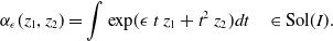 \begin{equation*} \alpha_\epsilon(z_1,z_2) = \int {\textrm{exp}} (\epsilon\ t\ z_1 + t^2\ z_2) dt \quad \in {\textrm{Sol}}(I). \end{equation*}
By taking the limit for
 $\epsilon \rightarrow 0$
, this yields arbitrary functions
$\epsilon \rightarrow 0$
, this yields arbitrary functions
 $a(z_2)$
. These are among the solutions to
$a(z_2)$
. These are among the solutions to
 $I_0 = \langle \partial_1^2 \rangle $
. Other limit solutions are obtained via the reflection
$I_0 = \langle \partial_1^2 \rangle $
. Other limit solutions are obtained via the reflection
 $t \mapsto -t$
. Set
$t \mapsto -t$
. Set
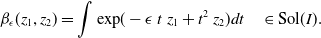 \begin{equation*} \beta_\epsilon(z_1,z_2) = \int {\textrm{exp}} (-\epsilon\ t\ z_1 + t^2\ z_2) dt \quad \in {\textrm{Sol}}(I). \end{equation*}
Note the similarity to the one-dimensional wave equation (1.5) with
 $c = \epsilon$
. The solution for
$c = \epsilon$
. The solution for
 $\epsilon = 0$
is given in (1.6). This is found from the integrals above by taking the following limit:
$\epsilon = 0$
is given in (1.6). This is found from the integrals above by taking the following limit:
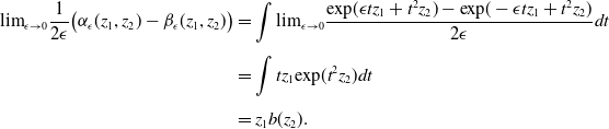 \begin{equation}\begin{aligned} {\textrm{lim}}_{\epsilon \rightarrow 0} \frac{1}{2 \epsilon} \bigl( \alpha_\epsilon(z_1,z_2) - \beta_\epsilon(z_1,z_2) \bigr) & = \int {\textrm{lim}}_{\epsilon \rightarrow 0}\frac{{\textrm{exp}}(\epsilon tz_1+t^2z_2)-{\textrm{exp}}(-\epsilon tz_1+t^2z_2)}{2\epsilon}dt\\[4pt] &= \int tz_1{\textrm{exp}}(t^2z_2) dt\\[4pt]& = z_1 b(z_2). \end{aligned}\end{equation}
We conclude that the general solution to
 $I_0$
equals
$I_0$
equals
 $ \phi(z_1,z_2) = a(z_2) + z_1 b(z_2)$
, where b is any function in one variable. The calculus limit in (6.1) realizes a scheme-theoretic limit in the sense of algebraic geometry. Namely, two lines in (1.7) converge to a double line in
$ \phi(z_1,z_2) = a(z_2) + z_1 b(z_2)$
, where b is any function in one variable. The calculus limit in (6.1) realizes a scheme-theoretic limit in the sense of algebraic geometry. Namely, two lines in (1.7) converge to a double line in
 $\mathbb{C}^2$
.
$\mathbb{C}^2$
.
Example 6.2 (
 $n=3$
). For
$n=3$
). For
 $\epsilon \not= 0$
consider the curve
$\epsilon \not= 0$
consider the curve
 $t \mapsto (\epsilon t^3, t^4, \epsilon^2 t^2)$
in
$t \mapsto (\epsilon t^3, t^4, \epsilon^2 t^2)$
in
 $\mathbb{C}^3$
. Its prime ideal equals
$\mathbb{C}^3$
. Its prime ideal equals
 $I_\epsilon = \langle \partial_1^2 - \partial_2 \partial_3, \partial_3^2 - \epsilon^4 \partial_2 \rangle$
. The solution space
$I_\epsilon = \langle \partial_1^2 - \partial_2 \partial_3, \partial_3^2 - \epsilon^4 \partial_2 \rangle$
. The solution space
 ${\textrm{Sol}}(I_\epsilon)$
consists of the functions
${\textrm{Sol}}(I_\epsilon)$
consists of the functions
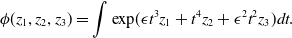 \begin{equation} \phi(z_1,z_2,z_3) = \int {\textrm{exp}}( \epsilon t^3 z_1 + t^4 z_2 + \epsilon^2 t^2 z_3) dt. \end{equation}
What happens to these functions when
 $\epsilon $
tends to zero? We address this question algebraically. The scheme-theoretic limit of the given ideal
$\epsilon $
tends to zero? We address this question algebraically. The scheme-theoretic limit of the given ideal
 $I_\epsilon$
is the ideal in Example 2.3. This is verified by a Gröbner basis computation (cf. [Reference Eisenbud18, Section 15.8]). Passing from ideals to their varieties, we see a toric curve in
$I_\epsilon$
is the ideal in Example 2.3. This is verified by a Gröbner basis computation (cf. [Reference Eisenbud18, Section 15.8]). Passing from ideals to their varieties, we see a toric curve in
 $\mathbb{C}^3$
that degenerates to a line with multiplicity four.
$\mathbb{C}^3$
that degenerates to a line with multiplicity four.
We claim that the formula in (2.9) arises from (6.2), just as in Example 6.1. Namely, set
 $i = \sqrt{-1}$
and let
$i = \sqrt{-1}$
and let
 $\phi_s \in {\textrm{Sol}}(I_\epsilon)$
be the function that is obtained from
$\phi_s \in {\textrm{Sol}}(I_\epsilon)$
be the function that is obtained from
 $\phi$
in (6.2) by replacing the parameter t with
$\phi$
in (6.2) by replacing the parameter t with
 $ i^s t$
. Then the following four functions on the left are solutions to
$ i^s t$
. Then the following four functions on the left are solutions to
 $I_\epsilon$
:
$I_\epsilon$
:
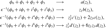 \begin{equation*}\begin{matrix} \phi_0+\phi_1+\phi_2+\phi_3 & \longrightarrow & a(z_2), \\[4pt] \epsilon^{-1} (\phi_0+i \phi_1+i^2 \phi_2+i^3 \phi_3) & \longrightarrow & z_1 b(z_2), \\[4pt] \epsilon^{-2} (\phi_0+i^2 \phi_1+i^4 \phi_2+i^6 \phi_3) & \longrightarrow & z_1^2 c'(z_2) + 2 z_3 c(z_2), \\[4pt] \epsilon^{-3} (\phi_0+i^3 \phi_1+i^6 \phi_2+i^9 \phi_3) & \longrightarrow & z_1^3 d'(z_2) + 6 z_1z_3 d(z_2).\end{matrix}\end{equation*}
The functions obtained as limits on the right are precisely the four summands seen in (2.9). Thus, the solution spaces to this family of PDE reflect the degeneration of the toric curve.
Such limits make sense also for modules. If a module
 $M_\epsilon \subseteq R^k$
depends on a parameter
$M_\epsilon \subseteq R^k$
depends on a parameter
 $\epsilon$
then we study its solution space
$\epsilon$
then we study its solution space
 ${\textrm{Sol}}(M_\epsilon)$
as
${\textrm{Sol}}(M_\epsilon)$
as
 $\epsilon $
tends to zero. Geometrically, we examine flat families of coherent sheaves on
$\epsilon $
tends to zero. Geometrically, we examine flat families of coherent sheaves on
 $\mathbb{C}^n$
or on
$\mathbb{C}^n$
or on
 $\mathbb{P}^{n-1}$
. A typical scenario comes from the action of the torus
$\mathbb{P}^{n-1}$
. A typical scenario comes from the action of the torus
 $(\mathbb{C}^*)^n$
, where Gröbner degenerations arise as limits under one-parameter subgroups. The limit objects are monomial ideals (for
$(\mathbb{C}^*)^n$
, where Gröbner degenerations arise as limits under one-parameter subgroups. The limit objects are monomial ideals (for
 $k=1$
) or torus-fixed submodules (for
$k=1$
) or torus-fixed submodules (for
 $k \geq 2$
). The next example illustrates their rich structure with an explicit family of torus-fixed submodules.
$k \geq 2$
). The next example illustrates their rich structure with an explicit family of torus-fixed submodules.
Example 6.3 (
 $n=2, k=3, l=6$
) Given a
$n=2, k=3, l=6$
) Given a
 $3 \times 6$
matrix A with random real entries, we set
$3 \times 6$
matrix A with random real entries, we set
 \begin{equation*} M = {\textrm{image}}_R \bigl( A \cdot {\textrm{diag}}(\partial_1,\partial_1^2,\partial_1^3, \partial_2,\partial_2^2,\partial_2^3)\bigr) \quad \subset \quad R^3. \end{equation*}
Then M is torus-fixed and
 $\mathfrak{m}$
-primary, where
$\mathfrak{m}$
-primary, where
 $\mathfrak{m} = \langle \partial_1,\partial_2 \rangle$
, and
$\mathfrak{m} = \langle \partial_1,\partial_2 \rangle$
, and
 ${\textrm{amult}}(M) = 10$
. A basis of
${\textrm{amult}}(M) = 10$
. A basis of
 ${\textrm{Sol}}(M)$
is given by ten polynomial solutions, namely the standard basis vectors
${\textrm{Sol}}(M)$
is given by ten polynomial solutions, namely the standard basis vectors
 $e_1,e_2,e_3$
, four vectors that are multiples of
$e_1,e_2,e_3$
, four vectors that are multiples of
 $z_1,z_1,z_2, z_2$
, and three vectors that are multiples
$z_1,z_1,z_2, z_2$
, and three vectors that are multiples
 $z_1^2, z_1 z_2, z_2^2$
. The reader is invited to verify this with Macaulay2. Here is the input for one concrete instance:
$z_1^2, z_1 z_2, z_2^2$
. The reader is invited to verify this with Macaulay2. Here is the input for one concrete instance:
R = QQ[x1,x2]
M = image matrix {{7*x1,5*x1^2,8*x1^3, 5*x2,9*x2^2,5*x2^3},
{8*x1,9*x1^2,8*x1^3, 4*x2,2*x2^2,4*x2^3},
{3*x1,2*x1^2,6*x1^3, 4*x2,4*x2^2,7*x2^3}}
solvePDE(M)
By varying the matrix A, and by extracting the vector multipliers of
 $1,z_1$
and
$1,z_1$
and
 $z_1^2$
, we obtain any complete flag of subspaces in
$z_1^2$
, we obtain any complete flag of subspaces in
 $\mathbb{C}^3$
. The vector multipliers of 1,
$\mathbb{C}^3$
. The vector multipliers of 1,
 $z_2$
, and
$z_2$
, and
 $z_2^2$
give us another complete flag of subspaces in
$z_2^2$
give us another complete flag of subspaces in
 $\mathbb{C}^3$
, and the multiplier of
$\mathbb{C}^3$
, and the multiplier of
 $z_1z_2$
gives us the intersection line of the planes corresponding to the multipliers of
$z_1z_2$
gives us the intersection line of the planes corresponding to the multipliers of
 $z_1$
and
$z_1$
and
 $z_2$
. This is illustrated in Figure 1. Thus flag varieties, with possible additional structure, appear naturally in such families.
$z_2$
. This is illustrated in Figure 1. Thus flag varieties, with possible additional structure, appear naturally in such families.
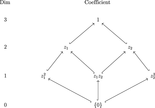
Figure 1. The coefficient vectors of the solutions to the PDE in Example 6.3 correspond to the above linear spaces with the given inclusions. We obtain two complete flags in
 $\mathbb{C}^3$
, along with one interaction between the two. Experts on quiver representations will take note.
$\mathbb{C}^3$
, along with one interaction between the two. Experts on quiver representations will take note.
The degenerations of ideals and modules we saw point us to Hilbert schemes and Quot schemes. Let us now also take a fresh look at Example 5.5. The modules M in that example form a flat family over the affine space
 $\mathbb{C}^5$
with coordinates
$\mathbb{C}^5$
with coordinates
 ${\bf c} = (c_1,c_2,c_3,c_4,c_5)$
. For
${\bf c} = (c_1,c_2,c_3,c_4,c_5)$
. For
 ${\bf c} = 0$
we obtain the PDE whose solution space equals
${\bf c} = 0$
we obtain the PDE whose solution space equals
 $\mathbb{C} \{e_1,z_1 e_1, z_1^2 e_1 \}$
. But, what happens when one of the coordinates of c tends to infinity? That limit exists in the Quot scheme.
$\mathbb{C} \{e_1,z_1 e_1, z_1^2 e_1 \}$
. But, what happens when one of the coordinates of c tends to infinity? That limit exists in the Quot scheme.
In our context, Hilbert schemes and Quot schemes serve as parameter spaces for primary ideals and primary modules. This was shown for ideals in [Reference Cid-Ruiz, Homs and Sturmfels11] and for modules in [Reference Chen and Cid-Ruiz9]. In what follows we shall discuss the latter case. Fix a prime ideal P of codimension c in
 $R = K[x_1,\ldots,x_n]$
. Write
$R = K[x_1,\ldots,x_n]$
. Write
 $\mathbb{K}$
for the field of fractions of the integral domain
$\mathbb{K}$
for the field of fractions of the integral domain
 $R/P$
, as in Line 6 of Algorithm 1. We write
$R/P$
, as in Line 6 of Algorithm 1. We write
 $u_1,\ldots,u_n$
for the images in
$u_1,\ldots,u_n$
for the images in
 $\mathbb{K}$
of the variables
$\mathbb{K}$
of the variables
 $x_1,\ldots,x_n$
in R. After possibly permuting these variables, we shall assume that
$x_1,\ldots,x_n$
in R. After possibly permuting these variables, we shall assume that
 $P \cap K[x_{c+1},\ldots,x_n] = \{0\}$
. The set
$P \cap K[x_{c+1},\ldots,x_n] = \{0\}$
. The set
 $\{u_{c+1},\ldots,u_n \}$
is algebraically independent over K, so it serves as
$\{u_{c+1},\ldots,u_n \}$
is algebraically independent over K, so it serves as
 $\mathcal{S}$
in Line 5.
$\mathcal{S}$
in Line 5.
Consider the formal power series ring
 $S = \mathbb{K}[[y_1,\ldots,y_c]]$
where
$S = \mathbb{K}[[y_1,\ldots,y_c]]$
where
 $y_1,\ldots,y_c$
are new variables. This is a local ring with maximal ideal
$y_1,\ldots,y_c$
are new variables. This is a local ring with maximal ideal
 $ \mathfrak{m} = \langle y_1,\ldots,y_c \rangle$
. We are interested in
$ \mathfrak{m} = \langle y_1,\ldots,y_c \rangle$
. We are interested in
 $\mathfrak{m}$
-primary submodules L of
$\mathfrak{m}$
-primary submodules L of
 $S^k$
. The quotient module
$S^k$
. The quotient module
 $S^k/L$
is finite-dimensional as a
$S^k/L$
is finite-dimensional as a
 $\mathbb{K}$
-vector space, and we write
$\mathbb{K}$
-vector space, and we write
 $\nu = {\textrm{dim}}_\mathbb{K}(S^k/L)$
for its dimension. The punctual Quot scheme is a parameter space whose points are precisely those modules. We denote the Quot scheme by
$\nu = {\textrm{dim}}_\mathbb{K}(S^k/L)$
for its dimension. The punctual Quot scheme is a parameter space whose points are precisely those modules. We denote the Quot scheme by
 \begin{equation} {\textrm{Quot}}^\nu (S^k) = \bigl\{ L \subset S^k \,:\, L\ \hbox{submodule with}\ {\textrm{Ass}}(L) = \mathfrak{m}\ \hbox{and}\ {\textrm{dim}}_\mathbb{K}(S^k/L) = \nu \bigr\}.\end{equation}
This is a quasiprojective scheme over
 $\mathbb{K}$
, i.e. it can be defined by a finite system of polynomial equations and inequations in a large but finite set of variables. Each solution to that system is one submodule L. This construction goes back to Grothendieck, and it plays a fundamental role in parametrizing coherent sheaves in algebraic geometry. While a constructive approach to Quot schemes exists, thanks to Skjelnes [Reference Skjelnes34], the problem remains to write defining equations for
$\mathbb{K}$
, i.e. it can be defined by a finite system of polynomial equations and inequations in a large but finite set of variables. Each solution to that system is one submodule L. This construction goes back to Grothendieck, and it plays a fundamental role in parametrizing coherent sheaves in algebraic geometry. While a constructive approach to Quot schemes exists, thanks to Skjelnes [Reference Skjelnes34], the problem remains to write defining equations for
 ${\textrm{Quot}}^\nu (S^k) $
in a computer-readable format, for small values of
${\textrm{Quot}}^\nu (S^k) $
in a computer-readable format, for small values of
 $c, k, \nu$
. A natural place to start would be the case
$c, k, \nu$
. A natural place to start would be the case
 $c=2$
, given that coherent sheaves supported at a smooth point on a surface are of considerable interest in geometry and physics [Reference Arbesfeld, Johnson, Lim, Oprea and Pandharipande1, Reference Baranovsky3, Reference Ellingsrud and Lehn20, Reference Henni, Jardim and Martins22].
$c=2$
, given that coherent sheaves supported at a smooth point on a surface are of considerable interest in geometry and physics [Reference Arbesfeld, Johnson, Lim, Oprea and Pandharipande1, Reference Baranovsky3, Reference Ellingsrud and Lehn20, Reference Henni, Jardim and Martins22].
The next two examples offer a concrete illustration of the concept of Quot schemes. We exhibit the Quot schemes that parametrize two families of linear PDE we encountered before.
Example 6.4 (
 $c=2,k=3,\nu=10$
) Consider the formal power series ring
$c=2,k=3,\nu=10$
) Consider the formal power series ring
 $S = \mathbb{K}[[y_1,y_2]]$
where
$S = \mathbb{K}[[y_1,y_2]]$
where
 $\mathbb{K}$
is any field. Replacing
$\mathbb{K}$
is any field. Replacing
 $\partial_1,\partial_2$
with
$\partial_1,\partial_2$
with
 $y_1,y_2$
in Example 6.3, every
$y_1,y_2$
in Example 6.3, every
 $ 3 \times 6$
matrix A over
$ 3 \times 6$
matrix A over
 $\mathbb{K}$
defines a submodule L of
$\mathbb{K}$
defines a submodule L of
 $S^3$
. The quotient
$S^3$
. The quotient
 $S^3/L$
is a 10-dimensional
$S^3/L$
is a 10-dimensional
 $\mathbb{K}$
-vector space, so L corresponds to a point in the Quot scheme
$\mathbb{K}$
-vector space, so L corresponds to a point in the Quot scheme
 $ {\textrm{Quot}}^{10} (S^3) $
. By varying A, we obtain a closed subscheme of
$ {\textrm{Quot}}^{10} (S^3) $
. By varying A, we obtain a closed subscheme of
 $ {\textrm{Quot}}^{10} (S^3) $
, which contains the complete flag variety we saw in Example 6.3.
$ {\textrm{Quot}}^{10} (S^3) $
, which contains the complete flag variety we saw in Example 6.3.
Example 6.5 For
 $S = \mathbb{K}[[y_1,y_2]]$
, the scheme
$S = \mathbb{K}[[y_1,y_2]]$
, the scheme
 $ {\textrm{Quot}}^{\nu} (S^k) $
is an irreducible variety of dimension
$ {\textrm{Quot}}^{\nu} (S^k) $
is an irreducible variety of dimension
 $k \nu - 1$
, by [Reference Baranovsky3, Theorem 2.2]. If
$k \nu - 1$
, by [Reference Baranovsky3, Theorem 2.2]. If
 $k=2, \nu = 3$
then this dimension is five. The affine space with coordinates c in Example 5.5 is a dense open subset W of
$k=2, \nu = 3$
then this dimension is five. The affine space with coordinates c in Example 5.5 is a dense open subset W of
 ${\textrm{Quot}}^3(S^2)$
, by [Reference Baranovsky3, Section 7].
${\textrm{Quot}}^3(S^2)$
, by [Reference Baranovsky3, Section 7].
For
 $k=1$
, the Quot scheme is the punctual Hilbert scheme
$k=1$
, the Quot scheme is the punctual Hilbert scheme
 ${\textrm{Hilb}}^\nu(S)$
; see [Reference Brianon6]. The points on this Hilbert scheme represent
${\textrm{Hilb}}^\nu(S)$
; see [Reference Brianon6]. The points on this Hilbert scheme represent
 $\mathfrak{m}$
-primary ideals of length
$\mathfrak{m}$
-primary ideals of length
 $\nu$
in
$\nu$
in
 $S = \mathbb{K}[[y_1,\ldots,y_c]]$
. It was shown in [Reference Cid-Ruiz, Homs and Sturmfels11, Theorem 2.1] that
$S = \mathbb{K}[[y_1,\ldots,y_c]]$
. It was shown in [Reference Cid-Ruiz, Homs and Sturmfels11, Theorem 2.1] that
 ${\textrm{Hilb}}^\nu(S)$
parametrizes the set of all P-primary ideals in R of multiplicity
${\textrm{Hilb}}^\nu(S)$
parametrizes the set of all P-primary ideals in R of multiplicity
 $\nu$
. This means that we can encode P-primary ideals in R by
$\nu$
. This means that we can encode P-primary ideals in R by
 $\mathfrak{m}$
-primary ideals in S, thus reducing scheme structures on any higher-dimensional variety to a scheme structure on a single point. This was generalized from ideals to submodules (
$\mathfrak{m}$
-primary ideals in S, thus reducing scheme structures on any higher-dimensional variety to a scheme structure on a single point. This was generalized from ideals to submodules (
 $k \geq 2$
) by Chen and Cid-Ruiz [Reference Chen and Cid-Ruiz9]. Geometrically, we encode coherent sheaves by those supported at one point, namely the generic point of V(P), corresponding to the field extension
$k \geq 2$
) by Chen and Cid-Ruiz [Reference Chen and Cid-Ruiz9]. Geometrically, we encode coherent sheaves by those supported at one point, namely the generic point of V(P), corresponding to the field extension
 $\mathbb{K}/K$
. Here is the main result from [Reference Chen and Cid-Ruiz9], stated for the polynomial ring R, analogously to [Reference Cid-Ruiz, Homs and Sturmfels11, Theorem 2.1].
$\mathbb{K}/K$
. Here is the main result from [Reference Chen and Cid-Ruiz9], stated for the polynomial ring R, analogously to [Reference Cid-Ruiz, Homs and Sturmfels11, Theorem 2.1].
Theorem 6.6 The following four sets of objects are in a natural bijective correspondence:
-
(a) P-primary submodules M in
$R^k$
of multiplicity
$\nu$
over P, -
(b)
$\mathbb{K}$
-points in the punctual Quot scheme
${\textrm{Quot}}^\nu \left(\mathbb{K}[[y_1,\ldots,y_c]]^k\right)$
, -
(c)
$\nu$
-dimensional
$\mathbb{K}$
-subspaces of
$\mathbb{K}[z_1,\ldots,z_c]^k$
that are closed under differentiation, -
(d)
$\nu$
-dimensional
$\mathbb{K}$
-subspaces of the Weyl–Noether module
$ \mathbb{K} \otimes_R D_{n,c}^k$
that are R-bimodules.


Moreover, any basis of the
 $\mathbb{K}$
-subspace (d) can be lifted to a finite subset
$\mathbb{K}$
-subspace (d) can be lifted to a finite subset
 $\mathcal{A} $
of
$\mathcal{A} $
of
 $ D_{n,c}^k$
such that
$ D_{n,c}^k$
such that
 \begin{equation}M = \bigl\{ m \in R^k \,:\, \delta \bullet m \in P\ \hbox{for all}\ \delta \in \mathcal{A} \bigr\}.\end{equation}
Here
 $D_{n,c}$
is the subalgebra of the Weyl algebra
$D_{n,c}$
is the subalgebra of the Weyl algebra
 $D_n$
consisting of all operators (4.3) with
$D_n$
consisting of all operators (4.3) with
 $s_{c+1} = \cdots = s_n = 0$
. This is a special case of (4.2). Elements in
$s_{c+1} = \cdots = s_n = 0$
. This is a special case of (4.2). Elements in
 $D_{n,c}$
are differential operators in
$D_{n,c}$
are differential operators in
 $\partial_{x_1},\ldots,\partial_{x_c}$
whose coefficients are polynomials in
$\partial_{x_1},\ldots,\partial_{x_c}$
whose coefficients are polynomials in
 $x_1,\ldots,x_n$
. Note that
$x_1,\ldots,x_n$
. Note that
 $D_{n,0} = R$
and
$D_{n,0} = R$
and
 $D_{n,n} = D_n$
. Equation (6.4) says that
$D_{n,n} = D_n$
. Equation (6.4) says that
 $\mathcal{A} $
is a differential primary decomposition for the primary module M. The Noetherian operators in
$\mathcal{A} $
is a differential primary decomposition for the primary module M. The Noetherian operators in
 $\mathcal{A}$
characterize membership in M. In this paper, however, we focus on the
$\mathcal{A}$
characterize membership in M. In this paper, however, we focus on the
 $\mathbb{K}$
-linear subspaces in item (c). By clearing denominators, we can represent such a subspace by a basis
$\mathbb{K}$
-linear subspaces in item (c). By clearing denominators, we can represent such a subspace by a basis
 $\mathcal{B}$
of elements in
$\mathcal{B}$
of elements in
 $K[x_1,\ldots,x_n][z_1,\ldots,z_c]$
. These are precisely the Noetherian multipliers needed for the integral representation of
$K[x_1,\ldots,x_n][z_1,\ldots,z_c]$
. These are precisely the Noetherian multipliers needed for the integral representation of
 ${\textrm{Sol}}(M)$
. In summary, Theorem 6.6 may be understood as a theoretical counterpart to Algorithm 1. The following example elucidates the important role played by the Quot scheme in our algorithm.
${\textrm{Sol}}(M)$
. In summary, Theorem 6.6 may be understood as a theoretical counterpart to Algorithm 1. The following example elucidates the important role played by the Quot scheme in our algorithm.
Example 6.7 (
 $n=4,c=2,k=3,\nu=10$
) Let P be the prime ideal in [Reference Cid-Ruiz, Homs and Sturmfels11, equation (1)]. Equivalently, P is the prime
$n=4,c=2,k=3,\nu=10$
) Let P be the prime ideal in [Reference Cid-Ruiz, Homs and Sturmfels11, equation (1)]. Equivalently, P is the prime
 $P_6$
in Example 2.4. The surface
$P_6$
in Example 2.4. The surface
 $V(P) \subset \mathbb{C}^4$
is the cone over the twisted cubic curve. Consider the point in
$V(P) \subset \mathbb{C}^4$
is the cone over the twisted cubic curve. Consider the point in
 ${\textrm{Quot}}^{10}(\mathbb{K}[[y_1,y_2]]^3)$
given by a matrix A as in Example 6.4. The bijection from (b) to (a) in Theorem 6.6 yields a P-primary submodule M of multiplicity 10 in
${\textrm{Quot}}^{10}(\mathbb{K}[[y_1,y_2]]^3)$
given by a matrix A as in Example 6.4. The bijection from (b) to (a) in Theorem 6.6 yields a P-primary submodule M of multiplicity 10 in
 $K[x_1,\ldots,x_4]^3$
. Generators for the module M are found by computing the inverse image under the map
$K[x_1,\ldots,x_4]^3$
. Generators for the module M are found by computing the inverse image under the map
 $\gamma$
, as shown in [Reference Chen and Cid-Ruiz9, equation (2)]. This step is the analogue for modules of the elimination that creates a large P-primary ideal Q from [Reference Cid-Ruiz, Homs and Sturmfels11, equation (5)]. Geometrically speaking, the 10-dimensional space of polynomial vectors that are solutions to the PDE in Example 6.3 encodes a coherent sheaf of rank 3 on the singular surface V(P).
$\gamma$
, as shown in [Reference Chen and Cid-Ruiz9, equation (2)]. This step is the analogue for modules of the elimination that creates a large P-primary ideal Q from [Reference Cid-Ruiz, Homs and Sturmfels11, equation (5)]. Geometrically speaking, the 10-dimensional space of polynomial vectors that are solutions to the PDE in Example 6.3 encodes a coherent sheaf of rank 3 on the singular surface V(P).
The ground field K in Section 5 need not be algebraically closed. In particular, we usually take
 $K=\mathbb{Q} $
when computing in Macaulay2. But this requires some adjustments in our results. For instance, Theorem 3.8 does not apply when the coordinates of
$K=\mathbb{Q} $
when computing in Macaulay2. But this requires some adjustments in our results. For instance, Theorem 3.8 does not apply when the coordinates of
 ${\bf u} \in \mathbb{C}^n$
are not in K. In such situations, we may take
${\bf u} \in \mathbb{C}^n$
are not in K. In such situations, we may take
 $\mathbb{K}$
to be an algebraic extension of K. We close with an example that shows the effect of the choice of ground field in a concrete computation.
$\mathbb{K}$
to be an algebraic extension of K. We close with an example that shows the effect of the choice of ground field in a concrete computation.
Example 6.8 (
 $n=k=2,l=3$
) Consider the module M given in Macaulay2 as follows:
$n=k=2,l=3$
) Consider the module M given in Macaulay2 as follows:
R = QQ[x1,x2]; M = image matrix {{x1,x1*x2,x2},{x2,x1,x1*x2}};
dim(R^2/M), degree(R^2/M), amult(M)
The output shows that
 ${\textrm{amult}}(M) = 5$
when
${\textrm{amult}}(M) = 5$
when
 $K = \mathbb{Q}$
, but
$K = \mathbb{Q}$
, but
 $\nu={\textrm{amult}}(M) = 6$
when
$\nu={\textrm{amult}}(M) = 6$
when
 $K = \mathbb{C}$
: Applying now the command solvePDE(M), we find the differential primary decomposition
$K = \mathbb{C}$
: Applying now the command solvePDE(M), we find the differential primary decomposition
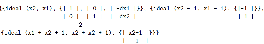
The module M has three associated primes over
 $K=\mathbb{Q}$
. The first gives three polynomial solutions, including
$K=\mathbb{Q}$
. The first gives three polynomial solutions, including
 $\displaystyle\binom{-z_1}{\phantom{-}z_2}$
. The second prime contributes
$\displaystyle\binom{-z_1}{\phantom{-}z_2}$
. The second prime contributes
 $\displaystyle\binom{-1}{\phantom{-}1}{\textrm{exp}}(z_1+z_2)$
, and the third gives
$\displaystyle\binom{-1}{\phantom{-}1}{\textrm{exp}}(z_1+z_2)$
, and the third gives
 $\displaystyle\binom{x_2+1}{1}{\textrm{exp}}(x_1 z_1 + x_2 z_2)$
, where
$\displaystyle\binom{x_2+1}{1}{\textrm{exp}}(x_1 z_1 + x_2 z_2)$
, where
 $(x_1,x_2)$
is
$(x_1,x_2)$
is
 $\frac{1}{2}(-1+\sqrt{3}i,-1-\sqrt{3}i)$
or
$\frac{1}{2}(-1+\sqrt{3}i,-1-\sqrt{3}i)$
or
 $\frac{1}{2}(-1-\sqrt{3}i,-1+\sqrt{3}i)$
. Here
$\frac{1}{2}(-1-\sqrt{3}i,-1+\sqrt{3}i)$
. Here
 $\mathbb{K} = \mathbb{Q}(\sqrt{3}i)$
is the field extension of
$\mathbb{K} = \mathbb{Q}(\sqrt{3}i)$
is the field extension of
 $K = \mathbb{Q}$
defined by the third associated prime.
$K = \mathbb{Q}$
defined by the third associated prime.
7. What next?
The results presented in this article suggest many directions for future study and research.
7.1. Special ideals and modules
One immediate next step is to explore the PDE corresponding to various specific ideals and modules that have appeared in the literature in commutative algebra and algebraic geometry.
One interesting example is the class of ideals studied recently by Conca and Tsakiris in [Reference Conca and Tsakiris14], namely products of linear ideals. A minimal primary decomposition for such an ideal I is given in [Reference Conca and Tsakiris14, Theorem 3.2]. It would be gratifying to find the arithmetic multiplicity
 ${\textrm{amult}}(I)$
and the solution spaces
${\textrm{amult}}(I)$
and the solution spaces
 ${\textrm{Sol}}(I)$
in terms of matroidal data for the subspaces in V(I).
${\textrm{Sol}}(I)$
in terms of matroidal data for the subspaces in V(I).
A more challenging problem is to compute the solution space
 ${\textrm{Sol}}(J)$
when J is an ideal generated by n power sums in
${\textrm{Sol}}(J)$
when J is an ideal generated by n power sums in
 $R = \mathbb{Q}[\partial_1,\ldots,\partial_n]$
. This problem is nontrivial even for
$R = \mathbb{Q}[\partial_1,\ldots,\partial_n]$
. This problem is nontrivial even for
 $n=3$
. To be more precise, we fix relatively prime integers
$n=3$
. To be more precise, we fix relatively prime integers
 $0 < a < b< c$
, and we consider the ideal
$0 < a < b< c$
, and we consider the ideal
 \begin{equation*} J_{a,b,c} = \langle \partial_1^a + \partial_2^a + \partial_3^a , \partial_1^b + \partial_2^b + \partial_3^b , \partial_1^c + \partial_2^c + \partial_3^c \rangle. \end{equation*}
If
 $(a,b,c) = (1,2,3) $
then
$(a,b,c) = (1,2,3) $
then
 $V(J_{1,2,3}) = \{0\}$
and
$V(J_{1,2,3}) = \{0\}$
and
 ${\textrm{Sol}}(J_{1,2,3})$
is a six-dimensional space of polynomials, spanned by the discriminant
${\textrm{Sol}}(J_{1,2,3})$
is a six-dimensional space of polynomials, spanned by the discriminant
 $(z_1-z_2)(z_1-z_3)(z_2-z_3)$
and its successive derivatives. In general, it is conjectured in [Reference Conca, Krattenthaler and Watanabe13] that
$(z_1-z_2)(z_1-z_3)(z_2-z_3)$
and its successive derivatives. In general, it is conjectured in [Reference Conca, Krattenthaler and Watanabe13] that
 $V(J_{a,b,c}) = \{0\}$
if and only if abc is a multiple of 6. If this holds then
$V(J_{a,b,c}) = \{0\}$
if and only if abc is a multiple of 6. If this holds then
 ${\textrm{Sol}}(J_{a,b,c})$
consists of polynomials. If this does not hold, then we must compute
${\textrm{Sol}}(J_{a,b,c})$
consists of polynomials. If this does not hold, then we must compute
 $V(J_{a,b,c})$
and extract the Noetherian multipliers from all associated primes of
$V(J_{a,b,c})$
and extract the Noetherian multipliers from all associated primes of
 $J_{a,b,c}$
. For instance, for
$J_{a,b,c}$
. For instance, for
 $(a,b,c) = (2,5,8)$
with
$(a,b,c) = (2,5,8)$
with
 $K=\mathbb{Q}$
, the arithmetic multiplicity is 38, one associated prime is
$K=\mathbb{Q}$
, the arithmetic multiplicity is 38, one associated prime is
 $\langle \partial_1+\partial_2+\partial_3,\partial_2^2 + \partial_2 \partial_3 + \partial_3^2 \rangle$
, and the largest degree of a polynomial solution is 10.
$\langle \partial_1+\partial_2+\partial_3,\partial_2^2 + \partial_2 \partial_3 + \partial_3^2 \rangle$
, and the largest degree of a polynomial solution is 10.
It will be worthwhile to explore the solution spaces
 ${\textrm{Sol}}(M)$
for modules M with special combinatorial structure. One natural place to start are syzygy modules. For instance, take
${\textrm{Sol}}(M)$
for modules M with special combinatorial structure. One natural place to start are syzygy modules. For instance, take
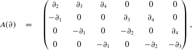 \begin{equation} A(\partial) \quad = \quad \begin{pmatrix} \partial_2 & \quad \partial_3 & \quad \partial_4 & \quad 0 & \quad 0 & \quad 0 \\[4pt]- \partial_1 & \quad 0 & \quad 0 & \quad \partial_3 & \quad \partial_4 & \quad 0 \\[4pt] 0 & \quad - \partial_1 & \quad 0 & \quad - \partial_2 & \quad 0 & \quad \partial_4 \\[4pt] 0 & \quad 0 & \quad - \partial_1 & \quad 0 & \quad -\partial_2 & \quad - \partial_3\end{pmatrix},\end{equation}
which is the first matrix in the Koszul complex for
 $n=4$
. Since
$n=4$
. Since
 ${\textrm{rank}}(A) = 3$
, the module
${\textrm{rank}}(A) = 3$
, the module
 $M = {\textrm{image}}_R(A)$
is supported on the entire space, i.e.
$M = {\textrm{image}}_R(A)$
is supported on the entire space, i.e.
 $V(M)=\mathbb{C}^4$
. Its solutions are the gradient vectors
$V(M)=\mathbb{C}^4$
. Its solutions are the gradient vectors
 $\nabla \alpha = \sum_{j=1}^4 \dfrac{\partial \alpha}{\partial z_j} e_j$
, where
$\nabla \alpha = \sum_{j=1}^4 \dfrac{\partial \alpha}{\partial z_j} e_j$
, where
 $\alpha = \alpha(z_1,z_2,z_3,z_4)$
ranges over all functions in
$\alpha = \alpha(z_1,z_2,z_3,z_4)$
ranges over all functions in
 $\mathcal{F}$
.
$\mathcal{F}$
.
Toric geometry [Reference Michałek and Sturmfels27, Chapter 8] furnishes modules whose PDE should be interesting. The initial ideals of a toric ideal with respect to weight vectors are binomial ideals, so the theory of binomial primary decomposition applies, and it gives regular polyhedral subdivisions as in [Reference Michałek and Sturmfels27, Theorem 13.28]. Nonmonomial initial ideals should be studied from the differential point of view. Passing to coherent sheaves, we may examine the modules representing toric vector bundles and their Gröbner degenerations. In particular, the cotangent bundle of an embedded toric variety, in affine or projective space, is likely to encompass intriguing PDE.
7.2. Linear PDE with polynomial coefficients
We discuss an application to PDE with non-constant coefficients, here taken to be polynomials. Our setting is the Weyl algebra
 $ D = \mathbb{C} \langle z_1,\ldots,z_n, \partial_1,\ldots,\partial_n \rangle$
. A linear system of PDE with polynomial coefficients is a D-module. For instance, consider a D-ideal I, that is, a left ideal in the Weyl algebra D. The solution space of I is typically infinite-dimensional.
$ D = \mathbb{C} \langle z_1,\ldots,z_n, \partial_1,\ldots,\partial_n \rangle$
. A linear system of PDE with polynomial coefficients is a D-module. For instance, consider a D-ideal I, that is, a left ideal in the Weyl algebra D. The solution space of I is typically infinite-dimensional.
We construct solutions to I with the method of Gröbner deformations [Reference Saito, Sturmfels and Takayama33, Chapter 2]. Let
 $w \in \mathbb{R}^n$
be a general weight vector, and consider the initial D-ideal
$w \in \mathbb{R}^n$
be a general weight vector, and consider the initial D-ideal
 ${\textrm{in}}_{(-w,w)}(I)$
. This is also a D-ideal, and it plays the role of Gröbner bases in solving polynomial equations. We know from [Reference Saito, Sturmfels and Takayama33, Theorem 2.3.3] that
${\textrm{in}}_{(-w,w)}(I)$
. This is also a D-ideal, and it plays the role of Gröbner bases in solving polynomial equations. We know from [Reference Saito, Sturmfels and Takayama33, Theorem 2.3.3] that
 ${\textrm{in}}_{(-w,w)}(I)$
is fixed under the natural action of the n-dimensional algebraic torus
${\textrm{in}}_{(-w,w)}(I)$
is fixed under the natural action of the n-dimensional algebraic torus
 $(\mathbb{C}^*)^n$
on the Weyl algebra D. This action is given in [Reference Saito, Sturmfels and Takayama33, equation (2.14)]. It gives rise to a Lie algebra action generated by the n Euler operators
$(\mathbb{C}^*)^n$
on the Weyl algebra D. This action is given in [Reference Saito, Sturmfels and Takayama33, equation (2.14)]. It gives rise to a Lie algebra action generated by the n Euler operators
 \begin{equation*} \theta_i = z_i \partial_i \quad {\textrm{for}}\ i = 1,2,\ldots,n. \end{equation*}
These Euler operators commute pairwise, and they generate a (commutative) polynomial subring
 $\mathbb{C}[\theta] = \mathbb{C}[\theta_1,\ldots,\theta_n]$
of the Weyl algebra D. If J is any torus-fixed D-ideal, then it is generated by operators of the form
$\mathbb{C}[\theta] = \mathbb{C}[\theta_1,\ldots,\theta_n]$
of the Weyl algebra D. If J is any torus-fixed D-ideal, then it is generated by operators of the form
 $x^a p(\theta) \partial^b$
where
$x^a p(\theta) \partial^b$
where
 $a,b \in \mathbb{N}^n$
. We define the falling factorial
$a,b \in \mathbb{N}^n$
. We define the falling factorial
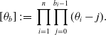 \begin{equation*} [\theta_b] \,:\!=\, \prod_{i=1}^n \prod_{j=0}^{b_i - 1} (\theta_i - j). \end{equation*}
The distraction
 $ \widetilde J $
is the ideal in
$ \widetilde J $
is the ideal in
 $\mathbb{C}[\theta]$
generated by all polynomials
$\mathbb{C}[\theta]$
generated by all polynomials
 $ [\theta_b] p(\theta-b) = x^b p(\theta) \partial^b $
, where
$ [\theta_b] p(\theta-b) = x^b p(\theta) \partial^b $
, where
 $ x^a p(\theta) \partial^b$
runs over a generating set of J. The space of classical solutions to J is equal to that of
$ x^a p(\theta) \partial^b$
runs over a generating set of J. The space of classical solutions to J is equal to that of
 $\widetilde J$
. This was exploited in [Reference Saito, Sturmfels and Takayama33, Theorem 2.3.11] under the assumption that J is holonomic, which means that
$\widetilde J$
. This was exploited in [Reference Saito, Sturmfels and Takayama33, Theorem 2.3.11] under the assumption that J is holonomic, which means that
 $\widetilde J$
is zero-dimensional in
$\widetilde J$
is zero-dimensional in
 $\mathbb{C}[\theta]$
. We here drop that assumption.
$\mathbb{C}[\theta]$
. We here drop that assumption.
Given any D-ideal I, we compute its initial D-ideal
 $J = {\textrm{in}}_{(-w,w)}(I)$
for
$J = {\textrm{in}}_{(-w,w)}(I)$
for
 $w \in \mathbb{R}^n$
generic. Solutions to I degenerate to solutions of J under the Gröbner degeneration given by w. We can often reverse that construction: given solutions to J, we lift them to solutions of I. Now, to construct all solutions of J we study the Frobenius ideal
$w \in \mathbb{R}^n$
generic. Solutions to I degenerate to solutions of J under the Gröbner degeneration given by w. We can often reverse that construction: given solutions to J, we lift them to solutions of I. Now, to construct all solutions of J we study the Frobenius ideal
 $F=\widetilde J$
. This is an ideal in
$F=\widetilde J$
. This is an ideal in
 $\mathbb{C}[\theta]$
.
$\mathbb{C}[\theta]$
.
We now describe all solutions to a given ideal F in
 $\mathbb{C}[\theta]$
. This was done in [33, Theorem 2.3.11] for zero-dimensional F. Ehrenpreis–Palamodov allows us to solve the general case. Here is our algorithm. We replace each operator
$\mathbb{C}[\theta]$
. This was done in [33, Theorem 2.3.11] for zero-dimensional F. Ehrenpreis–Palamodov allows us to solve the general case. Here is our algorithm. We replace each operator
 $\theta_i = z_i \partial_i$
by the corresponding
$\theta_i = z_i \partial_i$
by the corresponding
 $\partial_i$
. We then apply solvePDE to get the general solution to the linear PDE with constant coefficients. In that general solution, we now replace each coordinate
$\partial_i$
. We then apply solvePDE to get the general solution to the linear PDE with constant coefficients. In that general solution, we now replace each coordinate
 $z_i$
by its logarithm
$z_i$
by its logarithm
 ${\textrm{log}}(z_i)$
. In particular, each occurrence of
${\textrm{log}}(z_i)$
. In particular, each occurrence of
 ${\textrm{exp}}(u_1z_1+ \cdots +u_n z_n)$
is replaced by a formal monomial
${\textrm{exp}}(u_1z_1+ \cdots +u_n z_n)$
is replaced by a formal monomial
 $z_1^{u_1} \cdots z_n^{u_n}$
. The resulting expression represents the general solution to the Frobenius ideal F.
$z_1^{u_1} \cdots z_n^{u_n}$
. The resulting expression represents the general solution to the Frobenius ideal F.
Example 7.1 As a warm-up, we note that a function in one variable
 $z_2 $
is annihilated by the squared Euler operator
$z_2 $
is annihilated by the squared Euler operator
 $\theta_2^2 =z_2 \partial_2 z_2 \partial_2$
if and only if it is a
$\theta_2^2 =z_2 \partial_2 z_2 \partial_2$
if and only if it is a
 $\mathbb{C}$
-linear combination of 1 and
$\mathbb{C}$
-linear combination of 1 and
 ${\textrm{log}}(z_2)$
. Consider the Frobenius ideal given by Palamodov’s system [Reference Cid-Ruiz, Homs and Sturmfels11, Example 11]:
${\textrm{log}}(z_2)$
. Consider the Frobenius ideal given by Palamodov’s system [Reference Cid-Ruiz, Homs and Sturmfels11, Example 11]:
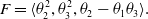 \begin{equation*} F = \langle \theta_2^2, \theta_3^2, \theta_2 - \theta_1 \theta_3 \rangle .\end{equation*}
To find all solutions to F, we consider the corresponding ideal
 $ \langle \partial_2^2, \partial_3^2, \partial_2 - \partial_1 \partial_3 \rangle $
in
$ \langle \partial_2^2, \partial_3^2, \partial_2 - \partial_1 \partial_3 \rangle $
in
 $\mathbb{C}[\partial_1,\partial_2,\partial_3]$
. By solvePDE, the general solution to that constant coefficient system equals
$\mathbb{C}[\partial_1,\partial_2,\partial_3]$
. By solvePDE, the general solution to that constant coefficient system equals
 \begin{equation*} \alpha(z_1) + z_2 \cdot \beta'(z_1) + z_3 \cdot \beta(z_1), \end{equation*}
where
 $\alpha$
and
$\alpha$
and
 $\beta$
are functions in one variable. We now replace
$\beta$
are functions in one variable. We now replace
 $z_i$
by
$z_i$
by
 ${\textrm{log}}(z_i)$
and we abbreviate
${\textrm{log}}(z_i)$
and we abbreviate
 $A(z_1) = \alpha({\textrm{log}}(z_1))$
and
$A(z_1) = \alpha({\textrm{log}}(z_1))$
and
 $B(z_1) = \beta({\textrm{log}}(z_1))$
. Thus, A and B are again arbitrary functions in one variable. We conclude that the general solution to the given Frobenius ideal F equals
$B(z_1) = \beta({\textrm{log}}(z_1))$
. Thus, A and B are again arbitrary functions in one variable. We conclude that the general solution to the given Frobenius ideal F equals
 \begin{equation*} \phi(z_1,z_2,z_3) = A(z_1) + z_1 \cdot {\textrm{log}}(z_2) \cdot B'(z_1) + {\textrm{log}}(z_3) \cdot B(z_1). \end{equation*}
This method can also be applied for
 $k \geq 2$
, enabling us to study solutions for any D-module.
$k \geq 2$
, enabling us to study solutions for any D-module.
7.3. Socle solutions
The solution space
 ${\textrm{Sol}}(M)$
to a system M of linear PDE is a complex vector space, typically infinite-dimensional. Our algorithm in Section 5 decomposes that space into finitely many natural pieces, one for each of the integrals in (2.6). The number
${\textrm{Sol}}(M)$
to a system M of linear PDE is a complex vector space, typically infinite-dimensional. Our algorithm in Section 5 decomposes that space into finitely many natural pieces, one for each of the integrals in (2.6). The number
 ${\textrm{amult}}(M)$
of pieces is a meaningful invariant from commutative algebra. Each piece is labeled by a polynomial
${\textrm{amult}}(M)$
of pieces is a meaningful invariant from commutative algebra. Each piece is labeled by a polynomial
 $B_{ij}({\bf x},{\bf z})$
in 2n variables, and it is parametrized by measures
$B_{ij}({\bf x},{\bf z})$
in 2n variables, and it is parametrized by measures
 $\mu_{ij}$
on the irreducible variety
$\mu_{ij}$
on the irreducible variety
 $V_i$
.
$V_i$
.
This approach does not take full advantage of the fact that
 ${\textrm{Sol}}(M)$
is an R-module where
${\textrm{Sol}}(M)$
is an R-module where
 $R = \mathbb{C}[\partial_1,\ldots,\partial_n]$
. Indeed, if
$R = \mathbb{C}[\partial_1,\ldots,\partial_n]$
. Indeed, if
 $\psi({\bf z})$
is any solution to M then so is
$\psi({\bf z})$
is any solution to M then so is
 $(\partial_i \bullet \psi)({\bf z})$
. So, if we list all solutions then
$(\partial_i \bullet \psi)({\bf z})$
. So, if we list all solutions then
 $\partial_i \bullet \psi$
is redundant provided
$\partial_i \bullet \psi$
is redundant provided
 $\psi$
is already listed. More precisely, we consider
$\psi$
is already listed. More precisely, we consider
 \begin{equation} {\textrm{Sol}}(M) / \langle \partial_1,\ldots,\partial_n \rangle {\textrm{Sol}}(M). \end{equation}
This quotient space is still infinite-dimensional over
 $\mathbb{C}$
, but it often has a much smaller description than
$\mathbb{C}$
, but it often has a much smaller description than
 ${\textrm{Sol}}(M)$
. A solution to M is called a socle solution if it is nonzero in (7.2). We pose the problem of modifying solvePDE so that the output is a minimal subset of Noetherian multipliers which represent all the socle solutions. The solution will require the prior development of additional theory in commutative algebra, along the lines of [Reference Chen and Cid-Ruiz9, Reference Cid-Ruiz, Homs and Sturmfels11, Reference Cid-Ruiz and Sturmfels12].
${\textrm{Sol}}(M)$
. A solution to M is called a socle solution if it is nonzero in (7.2). We pose the problem of modifying solvePDE so that the output is a minimal subset of Noetherian multipliers which represent all the socle solutions. The solution will require the prior development of additional theory in commutative algebra, along the lines of [Reference Chen and Cid-Ruiz9, Reference Cid-Ruiz, Homs and Sturmfels11, Reference Cid-Ruiz and Sturmfels12].
The situation is straightforward in the case of Theorem 3.8 when the support V(M) is finite. Here the space
 ${\textrm{Sol}}(M)$
is finite-dimensional, and it is canonically isomorphic to the vector space dual of
${\textrm{Sol}}(M)$
is finite-dimensional, and it is canonically isomorphic to the vector space dual of
 $R^k/M$
, as shown in [Reference Oberst30]. Finding the socle solutions is a computation using linear algebra over
$R^k/M$
, as shown in [Reference Oberst30]. Finding the socle solutions is a computation using linear algebra over
 $K = \mathbb{C}$
, similar to the three steps after Proposition 3.7. For instance, let
$K = \mathbb{C}$
, similar to the three steps after Proposition 3.7. For instance, let
 $k=1$
and suppose that I is a homogeneous ideal in R. The socle solutions are sometimes called volume polynomials [Reference Saito, Sturmfels and Takayama33, Lemma 3.6.20]. The most desirable case arises when I is Gorenstein. Here the socle solution is unique up to scaling, and it fully characterizes I. For instance, consider the power sum ideal
$k=1$
and suppose that I is a homogeneous ideal in R. The socle solutions are sometimes called volume polynomials [Reference Saito, Sturmfels and Takayama33, Lemma 3.6.20]. The most desirable case arises when I is Gorenstein. Here the socle solution is unique up to scaling, and it fully characterizes I. For instance, consider the power sum ideal
 $\langle \sum_{i=1}^n \partial_i^s \,:\, s=1,\ldots,n \rangle$
. This is Gorenstein with volume polynomial
$\langle \sum_{i=1}^n \partial_i^s \,:\, s=1,\ldots,n \rangle$
. This is Gorenstein with volume polynomial
 $\Delta = \prod_{1 \leq i < j \leq n} (z_i-z_j)$
. For
$\Delta = \prod_{1 \leq i < j \leq n} (z_i-z_j)$
. For
 $n=3$
, the ideal I is
$n=3$
, the ideal I is
 $J_{1,2,3}$
in Subsection 7.1. Here
$J_{1,2,3}$
in Subsection 7.1. Here
 ${\textrm{Sol}}(I)$
is a
${\textrm{Sol}}(I)$
is a
 $\mathbb{C}$
-vector space of dimension
$\mathbb{C}$
-vector space of dimension
 $n!$
. However, as an R-module, it is generated by a single polynomial
$n!$
. However, as an R-module, it is generated by a single polynomial
 $\Delta$
. A future version of solvePDE should simply output
$\Delta$
. A future version of solvePDE should simply output
 ${\textrm{Sol}}(I) = R \Delta$
.
${\textrm{Sol}}(I) = R \Delta$
.
It is instructive to revisit the general solutions to PDE we presented in this paper and to highlight the socle solutions for each of them. For instance, in Example 2.3, we have
 ${\textrm{amult}}(I) = 4$
but only one of the four Noetherian multipliers
${\textrm{amult}}(I) = 4$
but only one of the four Noetherian multipliers
 $B_i$
gives a socle solution. The last summand in (2.9) gives the socle solutions. The first three summands can be obtained from the last summand by taking derivatives. What are the socle solutions in Example 2.4?
$B_i$
gives a socle solution. The last summand in (2.9) gives the socle solutions. The first three summands can be obtained from the last summand by taking derivatives. What are the socle solutions in Example 2.4?
7.4. From calculus to analysis
The storyline of this paper is meant to be accessible for students of multivariable calculus. These students know how to check that (1.9) is a solution to (1.8). The derivations in Examples 2.3, 2.4, 5.1, 5.2, 6.1, 6.3, and 6.8 are understandable as well. No prior exposure to abstract algebra is needed to follow these examples, or to download Macaulay2 and run solvePDE.
The objective of this subsection is to move beyond calculus and to build a bridge to advanced themes and current research in analysis. First of all, we ought to consider inhomogeneous systems of linear PDE with constant coefficients. Such a system has the form
 \begin{equation}A(\partial) \bullet \psi({\bf z}) = f({\bf z}) ,\end{equation}
where A is a
 $k \times l$
matrix as before and f is a vector in
$k \times l$
matrix as before and f is a vector in
 $ \mathcal{F}^l$
, where
$ \mathcal{F}^l$
, where
 $\mathcal{F}$
is a space of functions or distributions. Writing
$\mathcal{F}$
is a space of functions or distributions. Writing
 $a_i$
for the ith column of A, the system (7.3) describes vectors
$a_i$
for the ith column of A, the system (7.3) describes vectors
 $\psi = (\psi_1,\ldots,\psi_k)$
with
$\psi = (\psi_1,\ldots,\psi_k)$
with
 $a_i \bullet \psi = f_i$
for
$a_i \bullet \psi = f_i$
for
 $i=1,\ldots,l$
. The study of the inhomogeneous system (7.3) is a major application of Theorem 2.2. We see this in Palamodov’s book [Reference Palamodov32, Chapter VII], but also in the work of Oberst who addresses the “canonical Cauchy problem” in [Reference Oberst28, Section 5]. An important role is played by the syzygy module
$i=1,\ldots,l$
. The study of the inhomogeneous system (7.3) is a major application of Theorem 2.2. We see this in Palamodov’s book [Reference Palamodov32, Chapter VII], but also in the work of Oberst who addresses the “canonical Cauchy problem” in [Reference Oberst28, Section 5]. An important role is played by the syzygy module
 ${\textrm{ker}}_R(A) \subset R^l$
, whose elements are the R-linear relations on the columns
${\textrm{ker}}_R(A) \subset R^l$
, whose elements are the R-linear relations on the columns
 $a_1,\ldots,a_l$
. A necessary condition for solvability of (7.3) is that the Fourier transform of the right-hand side
$a_1,\ldots,a_l$
. A necessary condition for solvability of (7.3) is that the Fourier transform of the right-hand side
 $f = (f_1,\ldots,f_l)$
satisfies the same syzygies. Hörmander shows in [Reference Hörmander23, Theorem 7.6.13] that the converse is also true, under certain regularity hypotheses on f. Thus, the computation of syzygies and other homological methods (cf. [Reference Eisenbud18, Part III]) are useful for solving (7.3). Treves calls this Simple algebra in the general case [Reference Treves35, Section 3.1]. We point to his exact sequence in [Reference Treves35, equation (3.5)]. Syzygies can be lifted to D-modules [Reference Saito, Sturmfels and Takayama33, Section 2.4] via the Gröbner deformations in Subsection 7.2.
$f = (f_1,\ldots,f_l)$
satisfies the same syzygies. Hörmander shows in [Reference Hörmander23, Theorem 7.6.13] that the converse is also true, under certain regularity hypotheses on f. Thus, the computation of syzygies and other homological methods (cf. [Reference Eisenbud18, Part III]) are useful for solving (7.3). Treves calls this Simple algebra in the general case [Reference Treves35, Section 3.1]. We point to his exact sequence in [Reference Treves35, equation (3.5)]. Syzygies can be lifted to D-modules [Reference Saito, Sturmfels and Takayama33, Section 2.4] via the Gröbner deformations in Subsection 7.2.
Another issue is to better understand which collections of vectors
 $B_{ij}$
arise as Noetherian multipliers for some PDE. The analogous question for Noetherian operators of ideals is addressed in [Reference Cid-Ruiz, Homs and Sturmfels11, Theorem 3.1]. That result is essentially equivalent to the characterization in [Reference Hörmander23, Theorem 7.7.7] of spaces
$B_{ij}$
arise as Noetherian multipliers for some PDE. The analogous question for Noetherian operators of ideals is addressed in [Reference Cid-Ruiz, Homs and Sturmfels11, Theorem 3.1]. That result is essentially equivalent to the characterization in [Reference Hörmander23, Theorem 7.7.7] of spaces
 $\mathcal{A}$
of Noetherian operators for a primary module as being closed under the Lie bracket. More work on this topic is needed. This is related to the issue of primary fusion, discussed at the end of [Reference Cid-Ruiz and Sturmfels12, Section 5], which concerns the compatibility of minimal sets of Noetherian operators for associated primes that are contained in one another.
$\mathcal{A}$
of Noetherian operators for a primary module as being closed under the Lie bracket. More work on this topic is needed. This is related to the issue of primary fusion, discussed at the end of [Reference Cid-Ruiz and Sturmfels12, Section 5], which concerns the compatibility of minimal sets of Noetherian operators for associated primes that are contained in one another.
We end with a pointer to current research in calculus of variations by De Phillippis and collaborators in [Reference Arroyo-Rabasa, De Philippis, Hirsch and Rindler2, Reference De Phillippis and Rindler16]. Each solution
 $\mu$
to the PDE
$\mu$
to the PDE
 $A \bullet \mu = 0$
is a Radon measure on an open set in
$A \bullet \mu = 0$
is a Radon measure on an open set in
 $\mathbb{R}^n$
with values in
$\mathbb{R}^n$
with values in
 $\mathbb{R}^k$
. Such a measure
$\mathbb{R}^k$
. Such a measure
 $\mu$
is called A-free, and one is interested in the singular part
$\mu$
is called A-free, and one is interested in the singular part
 $\mu^s $
of
$\mu^s $
of
 $\mu$
. Analysts view solutions among smooth functions as classical and well-understood, and they care primarily about irregularities and their rectifiability. One studies
$\mu$
. Analysts view solutions among smooth functions as classical and well-understood, and they care primarily about irregularities and their rectifiability. One studies
 $\mu^s$
via the polar vector
$\mu^s$
via the polar vector
 $\dfrac{{\textrm{d}} \mu}{{\textrm{d}} |\mu|}$
in
$\dfrac{{\textrm{d}} \mu}{{\textrm{d}} |\mu|}$
in
 $\mathbb{R}^k$
. The main result in [Reference De Phillippis and Rindler16] states that this vector always lies in the wave cone
$\mathbb{R}^k$
. The main result in [Reference De Phillippis and Rindler16] states that this vector always lies in the wave cone
 $\Lambda_A$
. This is a real algebraic variety in
$\Lambda_A$
. This is a real algebraic variety in
 $\mathbb{R}^k$
which is an invariant of our module
$\mathbb{R}^k$
which is an invariant of our module
 $M = {\textrm{image}}_R(A)$
. When
$M = {\textrm{image}}_R(A)$
. When
 $A = {\textrm{curl}} $
as in (7.1), the wave cone is a Veronese variety, and the result is Alberti’s Rank-One Theorem. The article [Reference Arroyo-Rabasa, De Philippis, Hirsch and Rindler2] proves the same conclusion for more refined wave cones, and it offers a conjecture relating the geometry of wave cones to the singular supports of solutions [Reference Arroyo-Rabasa, De Philippis, Hirsch and Rindler2, Conjecture 1.6]. It would be interesting to compute these real varieties in practice and to learn about A-free measures from the output of solvePDE.
$A = {\textrm{curl}} $
as in (7.1), the wave cone is a Veronese variety, and the result is Alberti’s Rank-One Theorem. The article [Reference Arroyo-Rabasa, De Philippis, Hirsch and Rindler2] proves the same conclusion for more refined wave cones, and it offers a conjecture relating the geometry of wave cones to the singular supports of solutions [Reference Arroyo-Rabasa, De Philippis, Hirsch and Rindler2, Conjecture 1.6]. It would be interesting to compute these real varieties in practice and to learn about A-free measures from the output of solvePDE.
7.5. Numerical algebraic geometry
In applications, one often does not have access to an exact representation of a problem, but rather some approximation with possible errors introduced by measurements or finite-precision arithmetic. The last decade of developments in numerical algebraic geometry [Reference Bates, Hauenstein, Sommese and Wampler4] provides tools for the numerical treatment of such polynomial models. In that paradigm, a prime ideal
 $P \subset \mathbb{C}[\mathbf{x}]$
is represented by a witness set, i.e. a set of
$P \subset \mathbb{C}[\mathbf{x}]$
is represented by a witness set, i.e. a set of
 $\textrm{deg}(P)$
points approximately on
$\textrm{deg}(P)$
points approximately on
 $V(P) \cap L$
, where L is a generic affine-linear space of dimension
$V(P) \cap L$
, where L is a generic affine-linear space of dimension
 $c = \textrm{codim}(P)$
. Similarly, radical ideals are collections of witness sets corresponding to irreducible components. Dealing with general ideals and modules is much more subtle, since these have embedded primes. One idea, pioneered by Leykin [Reference Leykin24], is to consider deflations of ideals. Modules were not considered in [Reference Leykin24]. Deflation has the effect of exposing embedded and nonreduced components as isolated components, which can subsequently be represented using witness sets. One drawback is that the deflated ideal lies in a polynomial ring with many new variables.
$c = \textrm{codim}(P)$
. Similarly, radical ideals are collections of witness sets corresponding to irreducible components. Dealing with general ideals and modules is much more subtle, since these have embedded primes. One idea, pioneered by Leykin [Reference Leykin24], is to consider deflations of ideals. Modules were not considered in [Reference Leykin24]. Deflation has the effect of exposing embedded and nonreduced components as isolated components, which can subsequently be represented using witness sets. One drawback is that the deflated ideal lies in a polynomial ring with many new variables.
We advocate the systematic development of numerical methods for linear PDE with constant coefficients. Noetherian operators and multipliers can be used to represent arbitrary ideals and modules. For each prime P, both the field
 $\mathbb{K}=\textrm{Frac}(R/P)$
and the spaces in (4.8) should be represented purely numerically. Along the way, one would extend the current repertoire of numerical algebraic geometry to modules and their coherent sheaves.
$\mathbb{K}=\textrm{Frac}(R/P)$
and the spaces in (4.8) should be represented purely numerically. Along the way, one would extend the current repertoire of numerical algebraic geometry to modules and their coherent sheaves.
First steps toward the numerical encoding of affine schemes were taken in [Reference Chen, Härkönen, Krone and Leykin10], for ideals I with no embedded primes. The key observation is that the coefficients of the Noetherian operators for the P-primary component of I can be evaluated at a point
 ${\bf u} \in V(P)$
using only linear algebra over
${\bf u} \in V(P)$
using only linear algebra over
 $\mathbb{C}$
. This linear algebra step can be carried out purely numerically.
$\mathbb{C}$
. This linear algebra step can be carried out purely numerically.
Inspired by this, we propose a numerical representation of an arbitrary module
 $M \subseteq R^k$
. Let
$M \subseteq R^k$
. Let
 $(P_i, \mathcal{S}_i, \mathcal{A}_i)$
be a differential primary decomposition as in Theorem 4.3. Assuming the ability to sample generic points
$(P_i, \mathcal{S}_i, \mathcal{A}_i)$
be a differential primary decomposition as in Theorem 4.3. Assuming the ability to sample generic points
 $\mathbf{u}_i \in V(P_i)$
, we encode the sets
$\mathbf{u}_i \in V(P_i)$
, we encode the sets
 $\mathcal{A}_i$
by their point evaluations
$\mathcal{A}_i$
by their point evaluations
 $\mathcal{A}_i(\mathbf{u}_i) = \{ A(\mathbf{u}_i, \mathbf{\partial_\mathbf{x}}) \,:\, A(\mathbf{x}, \partial_\mathbf{x}) \in \mathcal{A}_i \}$
. Each evaluated operator
$\mathcal{A}_i(\mathbf{u}_i) = \{ A(\mathbf{u}_i, \mathbf{\partial_\mathbf{x}}) \,:\, A(\mathbf{x}, \partial_\mathbf{x}) \in \mathcal{A}_i \}$
. Each evaluated operator
 $ A(\mathbf{u}_i, \mathbf{\partial_\mathbf{x}})$
gives an exponential solution
$ A(\mathbf{u}_i, \mathbf{\partial_\mathbf{x}})$
gives an exponential solution
 $B(\mathbf{u}_i, \mathbf{z}) \exp(\mathbf{u}_i^t \mathbf{z})$
to the PDE given by M via the correspondence in Proposition 4.8. We obtain a numerical module membership test: a polynomial vector
$B(\mathbf{u}_i, \mathbf{z}) \exp(\mathbf{u}_i^t \mathbf{z})$
to the PDE given by M via the correspondence in Proposition 4.8. We obtain a numerical module membership test: a polynomial vector
 $m \in R^k$
belongs to M with high probability if
$m \in R^k$
belongs to M with high probability if
 $A(\mathbf{u}_i, \partial_\mathbf{x}) \bullet m$
vanishes at the point
$A(\mathbf{u}_i, \partial_\mathbf{x}) \bullet m$
vanishes at the point
 $\mathbf{u}_i$
for all
$\mathbf{u}_i$
for all
 $A \in \mathcal{A}_i(\mathbf{u}_i)$
and
$A \in \mathcal{A}_i(\mathbf{u}_i)$
and
 $i = 1,\ldots,s$
. The exponential functions
$i = 1,\ldots,s$
. The exponential functions
 ${\bf z} \to B(\mathbf{u}_i, \mathbf{z}) \exp(\mathbf{u}_i^t \mathbf{z})$
, which depend on numerical parameters
${\bf z} \to B(\mathbf{u}_i, \mathbf{z}) \exp(\mathbf{u}_i^t \mathbf{z})$
, which depend on numerical parameters
 $\mathbf{u}_i$
, serve as an encoding of the infinite-dimensional
$\mathbf{u}_i$
, serve as an encoding of the infinite-dimensional
 $\mathbb{C}$
-vector space
$\mathbb{C}$
-vector space
 ${\textrm{Sol}}(M)$
.
${\textrm{Sol}}(M)$
.
Another potential research direction is the development of hybrid algorithms, where numerical information is used to speed up symbolic computations. Assuming the numerical approximations to be accurate enough, the output of a hybrid algorithm is exact. For Noetherian operators of ideals with no embedded components, this is explored in [Reference Chen, Härkönen, Krone and Leykin10], and it is already implemented in the Macaulay2 package NoetherianOperators [Reference Chen, Cid-Ruiz, Härkönen, Krone and Leykin8] using the command noetherianOperators(I, Strategy => “Hybrid”). It will be desirable to extend this hybrid method to the command solvePDE, in the full generality seen in Algorithm 1.
In conclusion, the numerical solution of partial differential equations is the key to computational science. The case of linear PDE with constant coefficients serves as a base case. We hope that the techniques described in this article will be useful for the future applications.


 Open access