


Introduction
Glaciers are forced downslope by driving stress due to gravitational collapse. The driving force is opposed by frictional drag, generally between the bedrock and the ice. Thebalance between these forces determines the extensional and compressional behaviour of a glacier and can be described in terms of a force budget. The method of balancing forces was developed and applied by Reference Whillans and van der VeenVan der Veen and Whillans (1989) and Whillans and others (1989) on Byrd Glacier, Antarctica, where they showed differences in basal drag in relation to the grounding zone of the glacier. This model has since been used successfully for various ice systems. Reference JanssonHøydal (1996) used the force-balance technique to show that bed topography has a great influence in controlling the direction of flow, even where the ice thickness exceeds 2000m (Jutulstraumen, Dronning Maud Land, Antarctica). Aided by force-budget calculations, Whillans and Reference Whillans and van der VeenVan der Veen (1997) pointed out the role of lateral drag in the dynamics of Ice Stream B, Antarctica, and Price and others (2002) found that the development of streaming ice flow depends on basal conditions far upstream from the actual ice-stream onset location. Reference PohjolaMayer and Huybrechts (1999) studied the ice-dynamic conditions across the grounding zone of Ekstromisen, East Antarctica. They found a clear transition between high and low basal drag as the ice transits from being grounded to become floating. It is clear that the analysis of force budgets provides valuable information on basal conditions for different ice systems.
Here we apply the force-budget technique, using the isothermal block-flow model, on Storglaciaren, Sweden, to investigate the ratio between basal drag and driving stress, τb/τd, in relation to bedrock topography. This index was defined by Reference Mayer and HuybrechtsMair and others (2001) while investigating the spatial patterns of glacier motion on Haut Glacier d’Arolla, Switzerland.
Storglaciaren has a long history of glaciological work, and its geometrical properties are well known (e.g. Jansson, 1996), but no thorough force-balance investigation has taken place on Storglaciaren in the past. However, Reference Hooke, Le, Calla, Holmlund, Nilsson and StroevenHooke and others (1989) studied the stress conditions and particularly the basal drag using a force balance of two small blocks of ice situated on either side of a bedrock threshold.The results from the latter study did not provide a full understanding of the dynamics across the bedrock threshold, a fact that motivated the present work.
Methods
Storglaciaren and data collection
Storglaciaren (Fig. 1) is a small valley glacier in the Scandinavian mountain range, northern Sweden (67°55'N, 18°35’ E). The bedrock topography of Storglaciaren is well known from previous radar soundings (Reference BjörnssonBjörnsson, 1981; Reference Eriksson, Björnsson, Herzfeld and HolmlundEriksson and others, 1993) providing necessary ice-depth information. Surface elevation data are from Holmund (1996). As seen in Figure 1a, Storglaciaren consists of four overdeepenings (at x ≈ 22600 m, x a 21500 m, x ≈20700m and x ≈20400m, respectively). In our study, we will concentrate on the two overdeepenings (OD1, x ≈22550, and OD2, x ≈22100) and the two bedrock ridges (R1, x ≈ 22800, and R2, x ≈ 22300) closest to the terminus (Fig. 1b). The bedrock of Storglaciaren consists of folded gneisses, amphibolites and diabase dykes and provides the geological control for the undulating topography (Reference Andreasson and GeeAndreasson and Gee, 1989).

Fig. 1. Drilled and measured stake net on Storglaciaren: (a) overview showing ice depth (m) and surface elevation (ma.s.l.) as dashed and solid contours, respectively; (b) subsection of area outlined with a rectangle in (a), showing basal topography as dashed contours (m a.s.l.). Black dots are initial stake positions, and the fix-point is marked with x in (a). Stakes are labelled in a row–column fashion from 11 to 76 and 101 to 121, as marked in (b). The locations of the bedrock ridges are between 110 and 115 (R1) and near stake row 3 (R2) separated by the overdeepenings (OD1and OD2). Earlier borehole study sites are marked with circles accompanied by drilling year (84, 85 and 86). Coordinates are in Swedish RT 90 0.0 gon with the y axis (south–north) perpendicular to the major ice-flow direction. The x axis is aligned with the major flow direction (west–east). The grid interval is 200 (100) m in the x(y) direction.
Surface velocity was measured by repeated differential global positioning system (DGPS) surveying of 63, 5m long, aluminium stakes drilled into the glacier ice in an approximately rectangular grid of 9 by 6 elements with 9 additional stakes placed at the terminus (Fig. 1a and b).
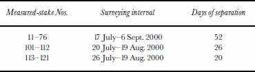
Stakes 100–121 were aligned roughly parallel to shear features at the glacier surface, distorting the down-glacier part of the grid. Stake grid coordinates were measured by kinematic surveying with a DGPS (Trimble 4600LS) during July–September 2000. Additional information on the GPS campaign is shown in Table 1. A fix point located at Tarfala Research Station (x = 23378.061, y =7535465.181) was occupied as a base station for all measurements. All GPS data were processed at Tarfala Research Station using Trimble GPSurvey v2.35 software.
Table 1. GPS campaign overview
Force-balance calculations
Storglaciaren is assumed to be isothermal, and the surface strain rates are assumed to be representative of those at depth. Taking resistive stresses constant with depth and neglecting vertical resistive stresses, we can write the so-called isothermal block-flow model for the horizontal directions, x and y, as:
where the driving stress, τdi, is balanced by the resistive stresses, τbi, ∂/∂x(HRxi) and ∂/∂y(HRyi) (Reference Whillans and van der VeenVan der Veen and Whillans, 1989). We will solve for basal drag, τb, which means the remaining terms need to be defined. The driving stress is calculated from the glacier geometry,
where p is ice density, g is gravitational acceleration, H is ice depth and z is surface elevation. The resistive stresses are written in terms of deviatoric stresses as follows (neglecting vertical resistive stresses):
The constitutive relation is applied to express the resistive stresses in terms of deviatoric stresses, invoking at the same time the inverse formulation of Nye’s generalization of Glen’s law:
where B is ice viscosity and n is the flow exponent for ice. The viscosity is calculated following Reference SandwellPohjola (1996), /β = β0 0 exp(T0/T), where T is ice temperature, β0 = 2.207 Pa a1/n and T0 = 3155 K, modified from Reference Hooke and LeHooke (1981). The strain rates are obtained from the gradients in the measured glacier surface velocities, U:
A force budget calculated using all 63 measured stakes, assuming they represent a period of similar surface velocities. In order to obtain better graphics for the maps of the dynamical properties, the velocity data were interpolated into a gridcell size of 20 m. The interpolation technique used to create the grid is described in Reference Van der Veen and WhillansSandwell (1987). Other constants used in the calculation are ice density, p = 900 kgm–3, ice temperature, T =0°C, ice-flow exponent,n =3, and gravitational acceleration, g = 9.82 m s–2.
Results
A force-budget calculation yields much information on different stress components (Van der Veen and Whillans, 1989). In this work, we restrict ourselves to showing the output that is central to our discussion: measured surface velocities, Ui, driving stress, τdi, and basal drag, τbi (i = x, y), and the index τb/τd using the resultant of τbi and τdi .
The overall velocity pattern of the x component, Ux (Fig. 2a), showing velocity increase over R2 and decrease downstream from it, agrees well with previous studies (Reference Hooke, Le, Pohjola, Jansson and KohlerHooke and others, 1989, Reference Iverson, Hanson, Le, Hooke and Jansson1992). The central parts of the glacier surface show velocities >20ma–1, with velocity maxima of 24.5 ma–1 found directly over R2. The y component, Uy (Fig. 2b), of the surface velocity shows a snaking flow, where a northerly flow shifts to a southerly flow at x ≈ 22200 m, with a shift back to northerly flow at x ≈ 22800 m. Values range from 4.6 m a 1 in a northerly direction to 3.9 ma– a southerly direction. This is probably due to the constriction imposed on the flow by R2 and has been recorded previously by Reference Hooke and LeHooke and others (1989).

Fig. 2. Velocity fields as interpolated from GPS measurements at the glacier surface (solid contours): (a) x component, Ux (m a–1); and (b) y component, Uy (m a–1). Arrows represent velocity resultants for each measured stake. Dashed contour lines are basal topography (m a.s.l.), and other map properties are as in Figure 1.
The resultant of the driving stress, τd (calculated from Equation (2)), is dominated by the x component (Fig. 3a) and exceeds 200 kPa in OD1 and decreases laterally as well as longitudinally. The maximum is located over OD1 where surface slopes are steep, and where ice is locally thicker. A slight tendency for increasing driving stress is found in the upstream extension of OD2. The y component of the driving stress shows relatively low negative values in OD1, which explains the turning of flow from a northerly direction above R2 into a southerly direction below R2 (Fig. 3a). At R1, the driving stress forces the flow northwards once again, which is also reflected in the measured surface velocities (Fig. 2b).

Fig. 3. (a) Calculated field of driving-stress resultants, τd (kPa) at the glacier bed (solid contours). (b) Calculatedfield of basal drag resultants, τb (kPa), at the glacier bed (solid contours). Arrows form a relative representation of the x and y components of driving stress and basal drag in (a) and (b), respectively. Other map properties are as in Figure 2.
The differences in the general pattern of the stress distribution and in the magnitude between the x and y components of basal drag (τbx and τby, calculated from Equation (1)) are similar to those of the driving stress. The x component reveals a zone of maximum basal drag in OD1, a local minimum on the lee side of R2 and high values in OD2 (Fig. 3b). The longitudinal basal drag decreases almost linearly from R1 towards the terminus. The y component of basal drag shows high resistance to the corresponding component of driving stress (Fig. 3a). Overall, the basal drag seems to balance the driving stress in the area of OD1 and laterally in an intermediate zone between the central and the marginal parts. Close to the valley walls, driving stress is exceeded by basal drag, probably because the ice is frozen to the bedrock (Reference HolmlundHolmlund and Eriksson, 1989).
τb/τd (Fig. 4) was calculated using the stress-field resultants and illustrates where the two balancing forces of basal drag and driving stress are different. The basal drag over R2, and especially on the lee side, is slightly lower (indicated as “low” in Fig. 4) than the driving stress, which explains why parts of the resisting forces must be non-local. Downslope of R2, basal drag is balanced by driving stress, while in central parts upstream of R2, basal drag exceeds the local driving stress (indicated as “high” in Fig. 4), indicating the action of non-local driving forces. Similar patterns are repeated at OD1 and R1. Reference Hooke, Le, Calla, Holmlund, Nilsson and StroevenHooke and others (1989) made a force-balance calculation based on six stakes between R2 and OD1 over the period July 1983–June 1985. A comparison between our results and those of Reference Hooke, Le, Calla, Holmlund, Nilsson and StroevenHooke and others (1989) shows similar values in these two studies. Hooke and others obtained average values for driving stress, τdx =145 kPa, and a basal drag of 91–170 kPa over the period. This can be compared with values from our calculation, of 150–200kPa in the same region. Before discussing these results, we discuss the uncertainty of the data.
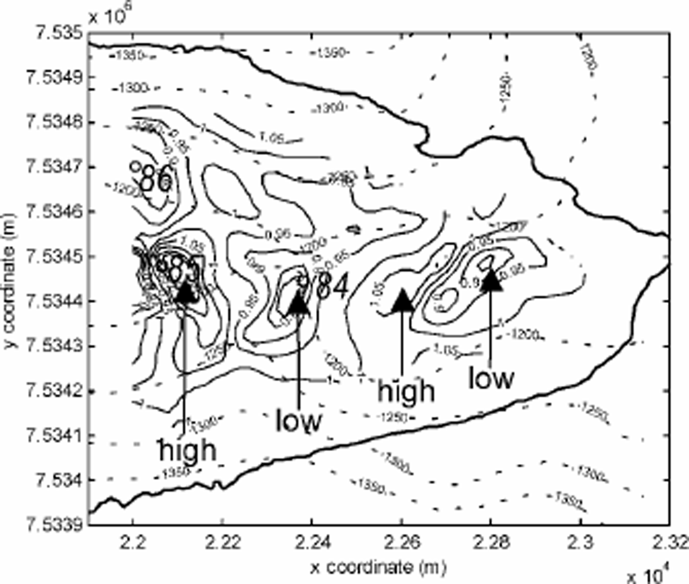
Fig. 4. The ratio of basal drag and driving stress, τb/τd , at the glacier bed (solid contours). Values 4 1 (high) indicate that the basal drag exceeds the driving stress, while values 5 1 (low) indicate that the basal drag is lower than the driving stress. Earlier borehole study sites are marked with circles accompanied by drilling year (8 4, 85 and 86). Other map properties are as in Figure 2.
Errors and Uncertainties
Errors in input data include measurement errors due to a combination of the human factor, instrumental faults, capacity limitations as well as missing data. Errors in the calculation technique spring from uncertainties in empirically determined physical constants and assumptions in boundary conditions. The limitations of the force-balance calculation are well presented in Reference Whillans and van der VeenVan der Veen and Whillans (1989). Herein we summarize the most important aspects.
The errors introduced by GPS measurements involve the instrument accuracy (±1 cm), the tendency for stakes to shake (±0.5 cm) at the time of measurement and the number of satellites entering the coordinate solution calculations (<0.1cm). However, the long time periods over which the stakes were measured reduce the instrumental and operational errors drastically for the glacier surface deformation dataset. Over a period of 52 days (when 42 out of 63 stakes were measured) the average ice surface movement along the centre line was 3.5 m, giving a maximum measurement error of 0.91% (2 6 0.016/3.5) or 0.22 ma–1. A rough estimation of the errors in the longitudinal strain rates (calculated over the stake grid size of 100 m) gives 0.0022 a–1 (0.22ma–1/100m) which is about 20% of the calculated strain rates in the area of interest.
The ice-depth information is most reliable at the centre line of the glacier, while, moving towards the margins, the risk of disturbed reflections reduces the quality of the data. A maximum error of ±5 m is assumed, although this is systematic and does not affect slope gradients to a large extent. The assumption of a 0°C ice temperature is correct for most of the glacier depth profile, but Reference Hooke, Le, Gould and BrzozowskiHooke and others (1983), Reference Holmlund and ErikssonHolmlund and Eriksson (1989) and R. Pettersson (unpublished information) have shown the presence of a cold surface layer (5 6 0 m) that affects the values of the dynamical parameters. Consequently, this cold surface layer possesses a higher viscosity, causing the ice to deform more slowly than the underlying temperate ice. Setting the ice temperature of the whole ice body to –4°C, the resulting basal drag field equals the basal drag field based on a temperature of 0°C. However, small differences of up to ±10 kPa appear near R1 and R2. The overall dynamical pattern does not appear different because of this.
In our calculation, we used a higher-density grid resolution than that of the measured stakes. The purpose of this was to obtain a better visualization in the output graphics of the strain and stress fields across the whole investigated ice body. A test run with a grid resolution equal to that of the actual measurement data, 100 6 100 m, was performed only to show the same patterns and magnitudes at that coarser spatial scale.
Discussion
The force-balance calculation shows a repetitive pattern in τb/τd as the ice flows over the bedrock ridges and into over-deepenings.This pattern is visible in Figure 4, and shows a rhythmical position of relatively high and low basal drags on the stoss and lee sides, respectively, of the bedrock thresholds. The wavelength of these relatively evenly distributed highs and lows is ∼400 m. Judging from the force-balance results, we find generally stickier basal conditions on the stoss side of the thresholds, and more lubricated conditions on the top and lee sides of the ridges. Ice flow is compressive upstream of the sticky areas, while flow is extensional between sticky and better-lubricated areas (not shown). The shift from compressional to extensional longitudinal strain is easily understood from continuum flow mechanics, where ice needs to accelerate when it moves from a stickier area to a more lubricated zone. The position of the centres of maximum extension found on the stoss sides of the ridges suggests that the acceleration of ice over bedrock ridges develops to compensate for decreased cross-sectional area, hence maintaining constant flux of ice. The accumulated force from ice upstream provides the driving force for the acceleration over the bedrock ridge.
We use the deformation of the surface area to find the stress pattern at the bed, but the englacial deformation pattern is an unknown (Reference Whillans and van der VeenVan der Veen and Whillans, 1989). Reference Hooke, Le, Holmlund and IversonHooke and others (1987,1992) investigated the englacial deformation patterns, or longitudinal and transverse vertical strain distribution (ἑxz, ἑyz), where Reference Hooke, Le, Holmlund and IversonHooke and others (1987) studied borehole deformation during July–September 1984 (borehole 84 in Fig. 1b) downstream of R2 at a point between our stakes 24 and 33. Reference Iverson, Hanson, Le, Hooke and JanssonHooke and others (1992) studied borehole deformation during July–September 1985 (borehole 85 in Fig. 1b) upstream of R2 at a point between our stakes 63 and 64. They also studied two boreholes in 1987 and 1988, respectively, in more lateral positions upstream of the area investigated in this work. An additional borehole (borehole 86 in Fig. 1b) was studied near stake 76, but results from this borehole were never published.
The general pattern from these studies was a higher component of basal sliding at the centre-line boreholes (4 8 1 % of surface velocity) than at the more lateral boreholes measured in 1987 and 1988 (generally 60–75 % of surface velocity). This is in accordance with our estimates of basal friction (Fig. 3b and 4), where basal drag is higher than driving stress at the glacier margins. The reason for the apparent increased lubrication at the centre of the glacier is that the lateral part is frozen to the bedrock, by higher water pressures at the centre and perhaps thicker till layers at the centre of the glacier. However, the results from till-deformation studies beneath Storglaciaren (e.g. Reference JanssonIverson and others, 1995) indicate that the till does not play an active role in the flow of the glacier. Hence, till deformation mechanisms can be ruled out in this case.
Boreholes 84 and 85, drilled on each side of R2, may help us to understand the basal dynamics at the bedrock ridge. A period of extrusion flow was identified in borehole 84 over part of the high-melt season (July) (Reference Hooke, Le, Calla, Holmlund, Nilsson and StroevenHooke and others, 1987), with basal velocities up to six times higher than surface velocities. Reference Hooke, Le, Calla, Holmlund, Nilsson and StroevenHooke and others (1987) suggested that decoupling of the ice from the bed by increased basal cavities filled with overpressurized water (i.e. decreased basal drag) may explain the episodic extrusion flow. No extrusion flow was found in borehole 85 (Reference Iverson, Hanson, Le, Hooke and JanssonHooke and others, 1992). When we compare the studies of internal deformation to our force-budget results, we find that borehole 85 was placed over an area of high basal drag, and that borehole 84 was placed over an area of low basal drag. Similarly, the area centred on borehole 86 showed episodic extrusion flow. Hence, it is likely that the episodic extrusion flow in borehole 84 was caused by the low basal drag on the lee side of the threshold. This can also be seen as a higher fraction of internal deformation in borehole 85 (82% basal sliding) compared to borehole 84 exhibiting about 92% basal sliding in two survey periods of non-extrusion flow during late summer. The cause of extrusion flow in borehole 86 cannot be described in terms of lee from any ridge, since it was measured upstream of R2. The position in the area of decreased basal drag is, however, similar to that of borehole 84.
The different studies referred to here were performed in different years but at roughly the same time of year. The velocity variations on Storglaciaren show a relatively similar pattern from year to year (Hooke and others, 1989; Reference JanssonJansson, 1995); hence, comparisons from year to year, especially when considering longer-term averages, are largely non-controversial. It is possible that the patterns revealed by the force budget vary with time, but we assume that the pattern is consistent from year to year, with larger intraannual variation. The bedrock topography and ice thickness are the major parameters that determine the pattern, and these are stable on a longer time-scale than is necessary for this study. Also, studies of the intra-annual variation in the basal drag pattern have shown that the wavelength of the pattern shown in Figure 6 is persistent within the year, but the amplitude varies with the seasons (Reference HedforsHedfors, 2002).
This force-budget analysis shows that the ice acceleration across R2 is induced by raised stresses on the stoss side and governed by low basal drags on the lee side. Low friction between the ice and underlying bedrock or till may develop as a result of intensive lubrication (Reference JanssonIverson and others, 1995). Reference JanssonJansson (1997) pointed out that the hydrological drainage pattern changes from englacial upstream of R2 to subglacial on the down-glacier side. This would explain the development of a local “slippery spot” downstream of R2 found in this study, suggesting a “pulling” of ice over the ridge.
Use of the isothermal block-flow model has proven valuable in the search for stress conditions underneath Storglaciaren. Most interesting is the relative pattern of the stress components; less important are their exact magnitudes. The major drawback of the model is that the viscous terms tend to be overestimated (since surface values are applied to the entire glacier thickness), so that basal drag becomes overestimated as well. Another extreme can be found when basal drag is set equal to driving stress. Hence, the actual value for basal drag may be expected to fall between these two set-ups. In the case of Storglaciaren, it is assumed that the isothermal model represents the actual environment since the obtained stress distributions strongly reflect the underlying bedrock topography. Also, consider that:
-
(i) repeated calculations for several datasets of surface velocity, covering different time periods, show similar stress distributions (with minor interesting differences; Reference HedforsHedfors, 2002);
-
(ii) high values of τb/τd are found towards the valley walls where the glacier is frozen to the bed (Reference PohjolaPohjola, 1993);
-
(iii) areas of low values of τb/τd align well with areas where the highest rates of basal sliding have been measured (Reference Hooke, Le, Calla, Holmlund, Nilsson and StroevenHooke and others, 1987); and
-
(iv) the minima in the calculated τb/τd are found in an area where the water-drainage system changes from englacial to subglacial (Reference JanssonJansson, 1997).
These facts help to establish confidence in the data-collection technique used, as well as in the force-budget method as applied to a small valley glacier.
Conclusion
The force-balance calculation shows a repetitive pattern in τb/rd as the ice flows over the bedrock ridges and into over-deepenings. Basal conditions are generally found to be stickier on the stoss side of the thresholds, and more lubricated on the top and lee sides of the ridges. When we compare the studies of internal deformation to our force-budget results, we find that borehole 85 was placed over an area of high basal drag and that borehole 84 was placed over an area of low basal drag. The lowest values of τb/τd are found over R1 which corresponds to the location where the water-drainage system changes from englacial to subglacial. The results from this study help to establish confidence in the force-budget method as applied to a small valley glacier.
Acknowledgements
A number of people at the Tarfala Research Station helped to collect and process the data, as well as being resourceful in solving logistical problems. We thank them for their contribution to this work. The whole project was graciously funded by a grant to J.H. from the Swedish Society for Anthropology and Geography (SSAG) and to P.J. from the Swedish Research Council (VR). The comments of R. C.A. Hindmarsh and two anonymous referees helped to improve this paper.


