


1. Introduction
Shock buffet brings a challenge to the wing design of modern large aircraft when flying in the commercially interesting transonic regime. Essentially, shock buffet is a manifestation of strong shock-wave/boundary-layer interaction, revealed through shock oscillations and intermittent boundary-layer separation. This sort of self-sustained unsteadiness will exert additional low-frequency aerodynamic loads, eventually limiting the flight envelope and potentially causing damage to the wing structure through the inevitable structural response, called buffeting, addressed through the certification requirements. Predicting shock-buffet onset early during wing design, and devising possible alleviation strategies, requires a clear understanding of its physical mechanisms and effective numerical methods, which is addressed herein. This work provides also a unique link between earlier biglobal stability studies on canonical geometries, to demonstrate consistency in the findings, and triglobal studies, using the same tools previously exercised by the authors (Timme & Thormann Reference Timme and Thormann2016; Timme Reference Timme2020) on practical finite wings with complex designs.
Early experiments identified a low-frequency shock motion linked to the flow dynamics on buffeting aerofoils (McDevitt, Levy & Deiwert Reference McDevitt, Levy and Deiwert1976; Levy Reference Levy1978). Lee (Reference Lee1990) investigated transonic flow on a supercritical aerofoil for Mach numbers between 0.5 and 0.8 and discerned unsteadiness at a Strouhal number of approximately 0.074, through measuring pressure fluctuation and unsteady aerodynamic force, and devised a first explanation. The aerofoil shock-buffet mechanism is now often explained by the shock interacting with upstream travelling acoustic waves generated at the trailing edge through shock-induced disturbances travelling downstream inside the separated boundary layer. This type of feedback loop was extensively examined by Hartmann, Feldhusen & Schröder (Reference Hartmann, Feldhusen and Schröder2013) and Feldhusen-Hoffmann et al. (Reference Feldhusen-Hoffmann, Statnikov, Klaas and Schröder2018) using time-resolved tomographic particle image velocimetry technology. Three-dimensional shock buffet in high Reynolds number flow presents distinct phenomena from two-dimensional experiments. Besides the two-dimensional characteristics, three-dimensional large-scale separation is observed with increasing angle of attack in experiments for a straight wing (Jacquin et al. Reference Jacquin, Molton, Deek, Maury and Soulevant2009) and wind-tunnel-scale aircraft (Masini, Timme & Peace Reference Masini, Timme and Peace2020a) models. It resembles the so-called stall cells documented in the flow of severe separation from low to high Reynolds numbers (Winkelmann & Barlow Reference Winkelmann and Barlow1980; He et al. Reference He, Gioria, Pérez and Theofilis2017; Plante et al. Reference Plante, Dandois, Beneddine, Laurendeau and Sipp2021). In addition to experiments, great flow detail in the transonic regime can also be provided by steady or unsteady simulations.
Numerical simulations on different aerofoils in high Reynolds number flow featuring shock oscillations showed that the flow can be approximated through solving the unsteady Reynolds-averaged Navier–Stokes (RANS) equations together with an appropriate turbulence model (Barakos & Drikakis Reference Barakos and Drikakis2000; Garbaruk et al. Reference Garbaruk, Shur, Strelets and Spalart2003; Thiery & Coustols Reference Thiery and Coustols2006), hence relying on the assumption of a separation of scales between the large-scale low-frequency coherent shock-buffet dynamics, accessible through the unsteady RANS method, and the small spatial and temporal scales of turbulence. The one-equation Spalart–Allmaras model is widely used in the simulation of turbulent transonic flow (Crouch, Garbaruk & Magidov Reference Crouch, Garbaruk and Magidov2007; Sartor, Mettot & Sipp Reference Sartor, Mettot and Sipp2015; Paladini et al. Reference Paladini, Beneddine, Dandois, Sipp and Robinet2019), while the suitability of various other models, such as linear and nonlinear eddy-viscosity two-equation models, is also widely addressed (Barakos & Drikakis Reference Barakos and Drikakis2000; Thiery & Coustols Reference Thiery and Coustols2006; Szubert et al. Reference Szubert, Grossi, Jimenez, Hoarau, Hunt and Braza2015; Giannelis, Levinski & Vio Reference Giannelis, Levinski and Vio2018). Besides using a RANS approach to study shock buffet, variants of detached-eddy simulation (Deck Reference Deck2005; Grossi, Braza & Hoarau Reference Grossi, Braza and Hoarau2014) and large-eddy simulation (Garnier & Deck Reference Garnier and Deck2010; Dandois, Mary & Brion Reference Dandois, Mary and Brion2018; Fukushima & Kawai Reference Fukushima and Kawai2018) are important alternatives due to increased insight into the unsteady flow physics. In addition to the typical low-frequency shock-buffet mode observed at high Reynolds numbers, several higher-frequency modes are reported in a moderate Reynolds number transonic flow over a laminar aerofoil using direct numerical simulation (Zauner, De Tullio & Sandham Reference Zauner, De Tullio and Sandham2019). Together with analysing the signal extracted from experiments and time-marching simulations, modal analysis using either an operator-based global stability method (Crouch et al. Reference Crouch, Garbaruk and Magidov2007; Sartor et al. Reference Sartor, Mettot and Sipp2015; Crouch, Garbaruk & Strelet Reference Crouch, Garbaruk and Strelet2019; Paladini et al. Reference Paladini, Beneddine, Dandois, Sipp and Robinet2019; Timme Reference Timme2020; Plante et al. Reference Plante, Dandois, Beneddine, Laurendeau and Sipp2021) or data-driven algorithms such as proper orthogonal decomposition and dynamic mode decomposition (Masini et al. Reference Masini, Timme and Peace2020a; Masini, Timme & Peace Reference Masini, Timme and Peace2020b; Zhao et al. Reference Zhao, Dai, Tian and Xiong2020) can be used to explore the flow mechanism.
Stability analysis was first shown to be an effective method in predicting the onset of two-dimensional aerofoil shock buffet by Crouch et al. (Reference Crouch, Garbaruk and Magidov2007). Those transonic-flow stability results on a NACA0012 aerofoil demonstrated good agreement with earlier experimental data (McDevitt & Okuno Reference McDevitt and Okuno1985). More recently, the ideas were successfully applied in the analysis of other aerofoils (Sartor et al. Reference Sartor, Mettot and Sipp2015; Zauner & Sandham Reference Zauner and Sandham2020) and three-dimensional infinite (Crouch et al. Reference Crouch, Garbaruk and Strelet2019; Paladini Reference Paladini2019; Paladini et al. Reference Paladini, Beneddine, Dandois, Sipp and Robinet2019; Plante et al. Reference Plante, Dandois, Beneddine, Laurendeau and Sipp2021) and finite (Timme & Thormann Reference Timme and Thormann2016; Timme Reference Timme2020) wings. In those infinite-wing shock-buffet studies, the authors predicted both the quasi-two-dimensional aerofoil mode and presented spatial spanwise-periodic modes in the framework of biglobal stability analysis. When using a symmetry (instead of periodic) boundary condition along the span, Iorio, González & Ferrer (Reference Iorio, González and Ferrer2014) only found the aerofoil mode in their triglobal investigation. Causes for not identifying the spanwise-periodic modes could lie in using small-aspect-ratio wings or imposing the symmetry boundary condition.
Importantly, detailed triglobal stability analysis on the infinite wing, both straight and swept, without assuming homogeneity in the span direction, is currently missing to link shock-buffet characteristics on the infinite wing, derived from biglobal studies, with those on the finite wing (Masini et al. Reference Masini, Timme and Peace2020a; Timme Reference Timme2020). Once the shock-buffet phenomenon appears, three-dimensional separation cells are formed on the suction side of the wing. Hence, bi- or triglobal analysis on a quasi-three-dimensional base flow in the absence of a spanwise flow field variation is not sufficient to describe the complete picture of perturbation modes. Only triglobal analysis can deal with an arbitrary three-dimensional flow field on a complex geometry, without an assumption on homogeneity in any spatial dimension, i.e. irrespective of assuming a homogeneous flow field in the spanwise direction, as done in biglobal studies. Herein, we are interested in understanding the fully three-dimensional perturbation dynamics, without simplifying assumptions, by describing the isolated impact of key geometric wing-sizing parameters (such as aspect ratio and sweep) and flow conditions (specifically angle of attack) in the formation and characteristics of the shock-buffet instability near onset. Section 2 introduces the definition of both infinite straight and swept-wing flow and the chosen numerical methods. Details of the base flows, and dependence on iterative and mesh convergence, are discussed in § 3. Triglobal stability results of infinite-wing shock buffet are presented in § 4.
2. Numerical set-up
2.1. Infinite-wing definition
Herein, we use the OAT15A aerofoil, which is the same profile used by Jacquin et al. (Reference Jacquin, Molton, Deek, Maury and Soulevant2009) in their experiments and by Sartor et al. (Reference Sartor, Mettot and Sipp2015), Paladini et al. (Reference Paladini, Beneddine, Dandois, Sipp and Robinet2019) and Crouch et al. (Reference Crouch, Garbaruk and Strelet2019) in their respective proper two-dimensional and biglobal three-dimensional stability analyses. As shown in figure 1, the aerofoil's two-dimensional baseline mesh is circular with a far-field radius of 100 chord lengths. Overall, the two-dimensional mesh is discretised by approximately  $35\,000$ points. The near-wall boundary-layer region is quasi-structured, with 75 points distributed in the wall-normal direction ensuring $y^+<1$, and 152 and 138 points discretise the suction and pressure sides of the aerofoil, respectively. An O-type meshing strategy was chosen for the region around the profile's blunt trailing edge. Unstructured triangular meshing is applied elsewhere towards the far-field boundary. While detailed mesh convergence in the aerofoil's $xz$-plane together with subtleties of the spatial discretisation and the choice of turbulence model have been presented in the literature (Barakos & Drikakis Reference Barakos and Drikakis2000; Deck Reference Deck2005; Thiery & Coustols Reference Thiery and Coustols2006; Nitzsche et al. Reference Nitzsche, Ringel, Kaiser and Hennings2019), we focus exclusively on the parameter choices in the spanwise direction, such as mesh resolution and finite aspect ratio. Straight-wing cases are defined by extruding the two-dimensional aerofoil mesh in spanwise direction to have different aspect ratios between
 ![]() and 10. An infinite span is achieved by using an appropriate spanwise-periodic boundary condition. The baseline extruded mesh for the infinite wing contains 20 points per unit length in span uniformly distributed, giving a total of approximately
and 10. An infinite span is achieved by using an appropriate spanwise-periodic boundary condition. The baseline extruded mesh for the infinite wing contains 20 points per unit length in span uniformly distributed, giving a total of approximately  $2.1\times 10^6$ points for our focus case with aspect ratio
 ![]() . The effect of spanwise resolution will be discussed in §§ 3.1 and 4.1 and the finite aspect ratio in § 3.3.
. The effect of spanwise resolution will be discussed in §§ 3.1 and 4.1 and the finite aspect ratio in § 3.3.

Figure 1. Mesh details showing  $(a)$ overall perspective of two-dimensional baseline mesh and $(b)$ magnified view near wing surface including periodic plane.
Swept wings are an integral part in designing modern large transport aircraft, on account of a better high-speed aerodynamic performance. Infinite swept wings are modelled herein by adjusting the direction and magnitude of the free-stream velocity vector, instead of modifying the wing shape or orientation, while ensuring constant flow conditions in the plane perpendicular to the wing's leading edge when varying the sweep angle. Figure 2 illustrates the flow past a wing with a non-zero sweep angle  $\varLambda$. Define reference Mach number $M_{\infty ,n}$, Reynolds number $Re_{\infty ,n}$ (based on chord length $c$) and angle of attack $\alpha$ in the perpendicular plane and use the transformations
 \begin{equation} \left. \begin{gathered} M_{\infty}=\frac{M_{\infty,n}}{\cos\varLambda}\sqrt{1-\sin^2\alpha\, \sin^2\varLambda}\\ Re_{\infty}=\frac{Re_{\infty,n}}{\cos\varLambda}\sqrt{1-\sin^2\alpha\,\sin^2\varLambda}\\ \gamma = \arctan(\tan\alpha\,\cos\varLambda) \end{gathered} \right\}. \end{equation}
As reference length, we use consistently the chord length  $c$ of the aerofoil defined perpendicular to the wing's leading edge.

Figure 2. Swept-wing flow set-up.
2.2. Governing equations and numerical methods
High Reynolds number turbulent transonic flow is described by the compressible RANS equations, coupled with a suitable turbulence model, given in non-dimensional, semi-discrete form as
 \begin{equation} \frac{\textrm{d}{\boldsymbol{u}}}{\textrm{d} t}= \mathcal{R}(\boldsymbol{u}) , \end{equation}
where the vector  $\mathcal {R}$ describes the nonlinear residual terms resulting from the spatial discretisation of the governing equations (and also includes the discrete control volumes, independent of time herein, when (2.2) is derived from a conservative integral form of the governing equations) and the conservative variables $\boldsymbol {u} = [\rho , \rho u,\rho v, \rho w, \rho E, \rho \tilde {\nu }]^\textrm {T}$ are defined for density, three Cartesian momentum components, total energy and the working variable of the turbulence model. Specifically, the Reynolds stresses are modelled through the Boussinesq approximation using the negative version of the Spalart–Allmaras turbulence model (Allmaras, Johnson & Spalart Reference Allmaras, Johnson and Spalart2012) to obtain the eddy viscosity.
The nonlinear governing equations (2.2), both steady state and time accurate, are solved using the TAU code of the German Aerospace Center (DLR), which is an industrial second-order code using a cell-vertex finite-volume formulation capable of dealing with complex geometries (Schwamborn, Gerhold & Heinrich Reference Schwamborn, Gerhold and Heinrich2006). The inviscid fluxes of the RANS equations are discretised using a central scheme with matrix artificial dissipation, whereas a first-order upwind scheme is used for those of the turbulence model. Gradients of flow variables, required for viscous fluxes and the source term of the turbulence model, are computed using the Green–Gauss approach. Besides the spanwise-periodic boundary condition introduced in the infinite-wing set-up, the viscous wall no-slip condition is strongly imposed on the solid walls of the wing and the far field is described as free-stream flow realised by the method of characteristics, consistent with interior-flux discretisation. As the time stepper to converge the system of equations to a steady state, we chose an explicit Runge–Kutta scheme with local time stepping and a geometric multigrid (normally on three grid levels) for convergence acceleration. We typically aim for a twelve orders of magnitude reduction in the norm of the density residual for steady-state iterations, while the reader should note the discussion in § 3. For unsteady time-marching simulation, which requires convergence to a pseudo-steady state in dual time, the second-order backward difference formula is adopted. Cauchy convergence control on the drag coefficient is specified with a minimum of 50 iterations in dual time per real time step, and a time-step size is defined to have approximately 1000 to 2000 time steps per period of a shock-buffet oscillation, resulting in a dimensional time-step size (with respect to free-stream velocity and chord length) of  $\Delta t=10^{-5}$ s to $10^{-4}$ s.
The steady-state RANS solution (fully coupled with the turbulence model), denoted  $\bar {\boldsymbol {u}}$ and satisfying $\mathcal {R}(\bar {\boldsymbol {u}})=0$, is used as base flow around which the linearised system is formed, leading to the eigenvalue problem
 \begin{equation} \lambda\hat{\boldsymbol{u}}=J\hat{\boldsymbol{u}} \end{equation}
through the exponential solution ansatz, where  $J = {\partial \mathcal {R}}/{\partial {\boldsymbol u}}$ is the flux Jacobian matrix and $\hat {\boldsymbol {u}}$ and $\lambda$ are eigenvector and eigenvalue, respectively. The eigenvalue $\lambda =\sigma +\textrm {i}\omega$ describes exponential growth or decay through $\sigma$ and an angular frequency of an oscillation through $\omega$. The eigenvector contains the complex-valued spatial amplitudes of the linear perturbation around the base flow, $\varepsilon \tilde {\boldsymbol {u}}={\boldsymbol {u}}-\bar {\boldsymbol {u}}$, where $\tilde {\boldsymbol {u}}=\hat {\boldsymbol {u}}\textrm {e}^{\varTheta }$. The phase function $\varTheta =\textrm {i}\beta y + \lambda t$ is specified by the chosen stability methodology (Theofilis Reference Theofilis2011) – in spanwise-uniform base flow, where $\overline {\rho v}\neq 0$ is permitted but $\partial \bar {\boldsymbol {u}}/\partial y\equiv 0$, assuming spanwise spatial periodicity in the perturbation dynamics, a biglobal approach can be chosen with $\beta \ge 0$ solving on a two-dimensional mesh in the $xz$-plane only, whereas triglobal analysis, setting $\beta =0$ and solving on an arbitrary mesh in three-dimensional space, makes no simplifying assumptions on the base flow, or indeed the modal response, whatsoever.
The latter triglobal stability approach, used throughout, has been implemented into the linear harmonic incarnation of the flow solver previously and its ability was demonstrated in Timme & Thormann (Reference Timme and Thormann2016) and Timme (Reference Timme2020). The implicitly restarted Arnoldi method (Sorensen Reference Sorensen1992), as implemented in the ARPACK library (Maschhoff & Sorensen Reference Maschhoff and Sorensen1996; Lehoucq, Sorensen & Yang Reference Lehoucq, Sorensen and Yang1998), is used to approximate a few but relevant eigenmodes in the outer iterations, whereby the Krylov sequence is computed for the shift-invert spectral transformation giving the matrix  $(J-\zeta I)^{-1}$ (instead of $J$) with $\zeta$ as user-specified complex-valued shift and $I$ as the identity matrix. This leads to the requirement of solving an inner linear system with the shifted coefficient matrix $(J-\zeta I)$ in each outer step using a preconditioned sparse iterative Krylov subspace solver (Parks et al. Reference Parks, de Sturler, Mackey, Johnson and Maiti2006; Xu, Timme & Badcock Reference Xu, Timme and Badcock2016).
The numerical strategy follows a first-discretise-then-linearise matrix-forming philosophy with a mostly hand-differentiated Jacobian matrix, corresponding to the chosen spatial discretisation including all boundary conditions and the turbulence model (without simplifications in the linearisation such as frozen eddy viscosity, cf. Thormann & Widhalm Reference Thormann and Widhalm2013). We refer to a mostly hand-differentiated matrix, because dealing with the linearised spanwise-periodic boundary condition in this work is a delicate matter. Since such an analytical boundary conditions is currently not available in the code, we made use of the existing analytical linearisation where possible (i.e. internal points not having periodic-plane points in their stencil) and implemented a numerical central finite-difference approach using graph colouring where necessary. Define as master periodic points those that are updated directly through solving the governing equations (i.e. those on one end of the otherwise finite span) and as shadow periodic points those updated indirectly through assigning the value of their paired master points (i.e. those on the other end). Care has to be taken that shadow periodic points are discarded in the Jacobian matrix altogether and any dependence on those points is transferred to the matrix position of the corresponding master periodic points.
For big problems with millions of degrees of freedom, the solution approach makes full use of the high performance parallel computing infrastructure of the underlying industrial flow solver. The investigation herein typically uses  $O(10 - 100)$ cores depending on the mesh size. The established numerical strategy combined with an industrial flow solver means that even practical non-canonical test cases at flight conditions can be investigated provided the decoupling of scales in high Reynolds number flow between the small scales of turbulence and the large scales dominating the dynamic system applies.
3. Base-flow classification
Flow conditions defined normal to the wing's leading edge (denoted by subscript  $n$) with reference free-stream Mach number $M_{\infty ,n} = 0.73$, chord Reynolds number $Re_{\infty ,n} = 3.2\times 10^6$ and angles of attack near the onset of shock buffet (similar to previous studies using the same OAT15A profile) are our concern. All data are in non-dimensional form, in particular, using the reference velocity $U_{\infty ,n}$ and chord length $c$, defined perpendicular to the wing's leading edge, unless explicitly stated otherwise.
3.1. Iterative and mesh convergence
A convergence study at a fixed angle of attack  $\alpha =3.5^\circ$ is performed to assess the impact of mesh resolution in the spanwise direction. A family of four meshes for a straight wing with aspect ratio
 ![]() is considered, featuring uniform spanwise spacings between
is considered, featuring uniform spanwise spacings between  $\Delta y=0.2$ and 0.025 giving between $n_y=15$ and 120 points along the span altogether. The density residual norm over iterations is examined for the steady-state simulations and presented in figure 3( $a$). Coefficients of lift and drag of the fully converged flow solutions, together with the relative errors, are summarised in table 1 while the respective convergence histories are provided in figure 3( $b$,
$b$, $c$). Besides the evident stages in the convergence behaviour discussed in the next paragraph, the fully converged results show clear differences in the terminal values of the lift and drag coefficients, linked to the attainable flow solution for a given mesh resolution. The coarsest mesh with 15 points along the span does not result in three-dimensional structures (as found for the other meshes) and consequently the lift coefficient is the highest. With the formation of said three-dimensional shock-distortion cells (one for the mesh with 30 points along the span and two for all finer meshes), the lift coefficient drops by 7.5 % (cf. table 1). A similar trend can be observed for the drag coefficient – note the competing components of drag when a local pocket of shock distortion is formed in combination with its downstream flow separation, as visualised in figure 4( $b{,}c$). Using the baseline mesh with 20 points per unit length of span, giving a resolution of $\Delta y=0.05$, only introduces a vanishing error in the integrated coefficients compared with the finest mesh of double the size. Importantly, this conclusion has to be amended when scrutinising the global mode results to follow.

Figure 3. Convergence history of ( $a$) density residual norm $\|{\mathcal {R}_\rho }\|$ and base-flow force coefficients of ( $b$) lift $\bar {C}_L$ and ( $c$) drag $\bar {C}_D$ for different spanwise spacings at angle of attack ${\alpha =3.5^\circ }$. Red bullets in ( $a$) relate to the snapshots in figure 4.
Table 1. Coefficients of lift and drag and relative error (with respect to finest mesh) from mesh convergence study at angle of attack  ${\alpha =3.5^\circ }$ for wing with aspect ratio
 ![]() .
.


Figure 4. Evolution of surface pressure coefficient  ${\bar {C}_p}$ on upper wing surface with respect to iteration number showing $(a)$
$(a)$  ${10\,000}$, $(b)$
$(b)$  ${40\,000}$ and $(c)$
$(c)$  ${120\,000}$ (marked by red bullets in figure 3 $a$) at angle of attack ${\alpha =3.5^\circ }$ for a straight wing with baseline mesh spacing $\Delta y=0.05$ and aspect ratio
 ![]() . Contour levels of
. Contour levels of  ${\bar {C}_p}$ are in the range ${[-1.5, 0]}$. The solid/dashed lines in ( $a$) highlight the spanwise skin-friction coefficient at $\bar C_{f_y}=\pm 10^{-7}$. The dashed-dotted lines in ( $b{,}c$) show zero skin friction to highlight the separation zone.
Looking more closely at the convergence history for the chosen baseline mesh, in combination with the corresponding surface pressure coefficient at three iteration numbers in figure 4, marked stages can be distinguished. To the naked eye, the surface pressure solution reveals no three-dimensional cellular pattern until approximately  $10\,000$ iterations (see figure 4 $a$), which describes the first, almost monotonic convergence phase in figure 3( $a$). This type of spanwise-uniform flow is found at a density residual level of approximately $\|\mathcal {R}_\rho \|= O(10^{-8})$, which is two orders of magnitude lower compared with typical convergence levels often used in industrial RANS simulations. More interestingly, an almost imperceptible cellular pattern with wavelength equal to the aerofoil chord length $c$ can be visualised through the spanwise skin-friction coefficient, $\bar C_{f_y}$, at a very low amplitude of $O(10^{-7})$. As will become clear in the following discussion, this subtly describes the leading unstable spanwise-periodic shock-distortion mode (with wavelength equal to the chord length), initially disturbing the otherwise spanwise-uniform base-flow solution. Continuing the steady-state iterations, the flow enters a stage where disturbances seem to grow. Here, the large-scale three-dimensional flow field is formed, as seen starting from $40\,000$ iterations in figure 4( $b$). This continues until nonlinear amplitude saturation helps establish the final steady state. Together with the convergence history of force coefficients, we can discern the impact of spanwise mesh resolution on the formation of the cellular pattern. Effectively, a minimum mesh resolution, and a minimum convergence threshold, is required to capture the cellular flow pattern along the span.
It should be noted that it was attempted during this study to obtain a spanwise-uniform solution at terminal convergence, for instance, by switching the time stepper to the code's usual implicit backward Euler method or by initialising the flow field using different aerofoil solutions converged to machine-epsilon values extruded along the span. Specifically, aerofoil solutions were obtained both on a proper two-dimensional grid and on a three-dimensional grid with one cell in the span direction and appropriate periodic boundary condition (sometimes called 2.5-dimensional), ensuring consistency in the spatial discretisation with respect to the proper three-dimensional approach throughout. Eventually, the shock distortion appears, which is consistent with the stability results to follow. To offer a possible explanation, converging to an unstable base state in the vicinity of an oscillatory global instability seems to be possible since the base flow is close to the time-averaged mean flow of the time-marched solution. This is not the case for the monotone shock-distortion mode.
3.2. Spanwise-uniform base flow on straight and swept wings
In an earlier experimental study (Jacquin et al. Reference Jacquin, Molton, Deek, Maury and Soulevant2009) on a wing with a small aspect ratio (![]() ), the flow was steady below an angle of attack
), the flow was steady below an angle of attack  $\alpha \lessapprox 3.1^\circ$ at the same nominal flow conditions studied herein. Surface oil flow visualisation revealed that the surface lines on the suction side of this wing are effectively two-dimensional before onset of shock buffet. In contrast, a three-dimensional flow structure can be observed behind the shock with angle of attack increased to $\alpha =3.5^\circ$. This behaviour can also be roughly examined using an appropriate RANS simulation. Figure 5 presents a surface flow visualisation of the fully converged RANS solution for the flow over the straight wing at a few angles of attack around the onset of unsteadiness. The formation of the three-dimensional cellular pattern for angles of attack beyond onset (based on the stability results to follow) is revealed. Figure 6 $(a)$ presents the pressure coefficient (extracted at the mid-span station) compared with these experiments at two selected angles of attack around the onset of shock buffet and the numerical two-dimensional aerofoil results (using a very similar version of the turbulence model) reproduced from Sartor et al. (Reference Sartor, Mettot and Sipp2015). The simulations at $\alpha =3.5^\circ$ are in good agreement with the wind-tunnel data at $\alpha =3.0^\circ$. The discrepancy is well documented and arises from the choice of turbulence model, which is further detailed in § 4.2. The corresponding integrated coefficients of lift and drag are shown in figure 6 $(b)$. Particularly for the lift coefficient, the very clear jump at angle of attack of approximately $\alpha =3.4^\circ$, coinciding with the formation of the shock distortion, is identified. For the drag coefficient, on the other hand, the jump is less pronounced due to the aforementioned competing drag contributions. The data points from Sartor et al. (Reference Sartor, Mettot and Sipp2015) are included for reference, noting that their two-dimensional aerofoil simulation cannot produce said shock distortion.

Figure 5. Fully converged surface pressure coefficient  ${\bar {C}_p}$, plotted in the range $[-1.5,0]$, on upper wing surface as a function of angle of attack for straight wing with baseline mesh spacing and aspect ratio
 ![]() . From (a) to (d) are angles of attack
. From (a) to (d) are angles of attack  ${\alpha =3.2^\circ }$ to $3.5^\circ$. The dashed-dotted lines highlight the separation zone by showing the zero skin-friction lines.

Figure 6. Base-flow results on straight wing with baseline mesh spacing and aspect ratio ![]() showing (
showing ( $a$) spanwise-uniform pressure coefficient compared with experiments from Jacquin et al. (Reference Jacquin, Molton, Deek, Maury and Soulevant2009) and steady-state two-dimensional aerofoil results from Sartor et al. (Reference Sartor, Mettot and Sipp2015) and ( $b$) lift and drag coefficient as function of angle of attack $\alpha$. Additional data points in $(b)$ for the lift coefficient $(\bullet )$ were also extracted from Sartor et al. (Reference Sartor, Mettot and Sipp2015).
These flow features can also be related to the non-monotonic trend in the convergence history in figure 7( $a$). Although steady-state RANS results are independent of time, useful insight can be extracted by analysing the residual history carefully to reveal the expected flow unsteadiness. The figure shows the complete convergence trend of the density residual norm of the steady RANS equations from low to high angles of attack around shock-buffet onset on the straight wing. Two types of nominally steady flow characteristics, specifically spanwise-uniform and -non-uniform base flow, can be identified depending on the level of convergence, as seen through the surface pressure coefficient in figures 4 and 5. For the straight-wing cases at angles of attack $\alpha =3.2^\circ$ and $3.3^\circ$, the simulations quickly converge to the defined tolerance of $\|\mathcal {R}_{\rho }\|=O(10^{-12})$. There is no three-dimensional cellular flow pattern visible on the wing surface as shown in figure 5. Interestingly, the iteration count grows dramatically when increasing the angle of attack to $\alpha =3.4^\circ$. This suggests that we are in the vicinity of a critical condition and it takes (substantially) more iterations to amplify an unstable (spanwise-periodic) mode with a positive growth rate close to zero. This statement will be supported in § 4.2 by using stability theory to extract dominant eigenmodes for the selected uniform base flow. As explained in § 3.1, for stability analysis at higher angles of attack $\alpha =3.4^\circ$ and $3.5^\circ$, we select the approximately uniform base flow observed at $10\,000$ iterations giving a minimum density residual norm of approximately $\|\mathcal {R}_{\rho }\|=O(10^{-8})$ from the initial, almost monotonic stage of convergence. Similar convergence level was reported by Crouch et al. (Reference Crouch, Garbaruk and Strelet2019).

Figure 7. Convergence history of density residual norm  $\|{\mathcal {R}_\rho }\|$ for wing with baseline mesh spacing and aspect ratio
 ![]() showing
showing  ${(a)}$ different angles of attack for straight wing and ${(b)}$ different sweep angles at angle of attack ${\alpha =3.5^\circ }$.
When the free-stream direction is not perpendicular to the leading edge of the wing, flow over a swept wing is described. Following (2.1), we ensure that the flow conditions perpendicular to the leading edge remain identical, independent of the sweep angle, for the different sweep angles discussed herein, specifically  $\varLambda = 5^\circ$, $10^\circ$, $20^\circ$ and $30^\circ$. Their convergence behaviour is compared with the straight wing in figure 7( $b$). The solution converges well, almost monotonically, for $\varLambda = 20^\circ$ and $30^\circ$ and, interestingly and in contrast to the straight wing, spanwise-uniform flow is found at terminal convergence. At the lower sweep angles of $\varLambda =5^\circ$ and $10^\circ$, convergence stalls, failing to reach the specified tolerance, and different methods, such as selective frequency damping (Åkervik et al. Reference Åkervik, Brandt, Henningson, Hœpffner, Marxen and Schlatter2006) or a stronger implicit Newton–Krylov solver (Yan et al. Reference Yan, Pan, Castiglioni, Hillewaert, Peiró, Moxey and Sherwin2021), should be explored in the future to find fully converged base flow in those cases. Close inspection of the corresponding non-converged flow fields suggests indecisiveness in either forming spanwise cellular structures as for sweep angle $\varLambda =0^\circ$ or convergence towards spanwise-uniform flow as for the two largest sweep angles investigated. However, similar to the discussion for the straight wing above, approximately uniform flow along the span is identified at convergence levels close to $\|\mathcal {R}_\rho \|= O(10^{-8})$. This statement will be further scrutinised in § 4.2.
3.3. Spanwise-non-uniform base flow on straight wing
Based on previous investigations (Jacquin et al. Reference Jacquin, Molton, Deek, Maury and Soulevant2009; Plante, Dandois & Laurendeau Reference Plante, Dandois and Laurendeau2020), three-dimensional shock-distortion patterns exist in post-onset shock-buffet conditions for the straight wing with aspect ratio ![]() . Taking the angle of attack
. Taking the angle of attack  $\alpha =3.5^\circ$ as an example, the simulation starts showing such three-dimensional cells along the span after approximately $40\,000$ iterations (see figure 4 $b$). The pronouncedness of cells continues to grow while the residual goes down, until the flow reaches the stage of nonlinear saturation. For a full account on the base flow, a more comprehensive study of the spanwise cells on wings with different aspect ratios between
 ![]() and
and  $10$ is shown in figure 8. Figure 9 illustrates the lift and drag coefficients, $\bar {C}_L$ and $\bar {C}_D$, and the size of each cell, $L$, measuring the distance between its two foci (highlighted by the exemplary red line in figure 8), varying with aspect ratio. There is one cell formed on the wing with aspect ratio
 ![]() , the size of which is smaller than the cells on wings with
, the size of which is smaller than the cells on wings with ![]() to 4. The cells are well developed on wings with
to 4. The cells are well developed on wings with ![]() , almost two times larger than on
, almost two times larger than on ![]() . The variation of the lift and drag coefficients with respect to the finite aspect ratio is less pronounced; the maximum difference between the wings with aspect ratio
. The variation of the lift and drag coefficients with respect to the finite aspect ratio is less pronounced; the maximum difference between the wings with aspect ratio ![]() and the highest aspect ratio is
and the highest aspect ratio is  $4.0\,\%$ for the lift coefficient and $1.7\,\%$ for the drag coefficient. Stability analysis will be discussed for aspect ratios
 ![]() , 5 and 10.
, 5 and 10.

Figure 8. Steady base-flow surface pressure coefficient  ${\bar {C}_p}$, plotted in the range $[-1.5,0]$, for wings with baseline mesh spacing and different aspect ratios at angle of attack ${\alpha =3.5^\circ }$.

Figure 9. Aspect-ratio dependence at machine-epsilon convergence (corresponding to figure 8) showing ( $a$) coefficients of lift $\bar {C}_L$ and drag $\bar {C}_D$ and ( $b$) cell size $L$.
$L$.
4. Triglobal shock-buffet stability results
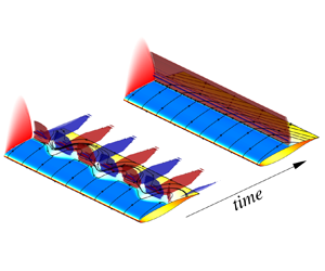
Based on the spanwise-uniform and -non-uniform steady-state base flows established in § 3, triglobal shock-buffet instability studies follow. First, we probe the numerical set-up to ensure it is robust and understood with respect to the various intricate parameter choices. Then, two types of global modes, specifically uniform and periodic in the spanwise direction, are investigated for the spanwise-uniform base flow on straight and swept wings. Accordingly, the modal characteristics of the non-uniform base flow, which describes the saturated state following a first bifurcation with spanwise-periodic monotone modes, are scrutinised. Finally, we interpret the findings from a time-domain perspective.
4.1. Sanity checks on numerical set-up
The primary purpose of scrutinising the solution approach when solving the triglobal three-dimensional linearised aerodynamic system with spanwise-periodic boundary conditions is to ensure robustness with respect to the main parameters of the numerical problem, focussing on the finite-difference step size when computing the periodic parts of the Jacobian matrix, finite aspect ratio and spanwise mesh resolution. Note that, even though we initially present our argumentation based on the eigenvalues  $\lambda$ only without visualising the corresponding eigenvectors $\hat {\boldsymbol {u}}$, the eigenvalues are indeed examined through the Rayleigh quotient, $\lambda =\hat {\boldsymbol {u}}^H J\hat {\boldsymbol {u}}$ (where eigenvector $\hat {\boldsymbol {u}}$ is scaled to unit length, $\hat {\boldsymbol {u}}^H\hat {\boldsymbol {u}}=1$, and superscript $H$ denotes the Hermitian transpose), implicitly verifying the eigenvector, too. These sanity checks focus on the spanwise-uniform base flow on the straight wing at angle of attack $\alpha =3.5^\circ$.
The effect of finite-difference step size,  $\varepsilon$, on the computed eigenmodes is scrutinised first for the case with baseline mesh spacing $\Delta y=0.05$ and aspect ratio
 ![]() . The step size defines the increment with respect to a local flow variable, as discussed by Mettot, Renac & Sipp (Reference Mettot, Renac and Sipp2014). Altogether, four different values of the step size are presented in figure 10
. The step size defines the increment with respect to a local flow variable, as discussed by Mettot, Renac & Sipp (Reference Mettot, Renac and Sipp2014). Altogether, four different values of the step size are presented in figure 10 $(a)$. Two shift positions, specifically $\zeta _1=0.45i$ and $\zeta _2=0.3$, are used here to identify the discrete aerofoil-type mode with higher frequency ( $\omega \approx 0.44$) and four monotone (i.e. zero frequency) shock-distortion modes of different wavelengths. Within the investigated range of step sizes, the impact on the numerical accuracy of the eigenvalues is virtually non-existent, which should be expected from such a graph-coloured approach. We will consistently use $\varepsilon =10^{-6}$ in the following and throughout.

Figure 10. Dependence of eigenmodes found in spanwise-uniform base flow on straight wing at angle of attack  $\alpha =3.5^\circ$ showing effect of ( $a$) finite-difference step size, $(b)$ aspect ratio and $(c)$ spanwise mesh spacing. The remaining main parameters in each case are kept at their reference values, specifically baseline mesh spacing $\Delta y=0.05$, aspect ratio
 ![]() and finite-difference step size
and finite-difference step size  $\varepsilon =10^{-6}$. Stability results for an alternative base flow constructed by extruding an aerofoil solution along the span ( $\times$), cf. figure 11 as well, and numerical data from Paladini et al. (Reference Paladini, Beneddine, Dandois, Sipp and Robinet2019) $(\bullet )$ are included in $(c)$.
A wide range of (essentially continuous) wavenumbers can be scrutinised in the framework of biglobal stability analysis. Hence, modes with (very) long, intermediate and short wavelengths have been found by Crouch et al. (Reference Crouch, Garbaruk and Strelet2019); Crouch, Garbaruk & Strelets (Reference Crouch, Garbaruk and Strelets2020), while contemplating the physical meaning of those short wavelength modes in the context of turbulence modelling, due to the spanwise length scales becoming similar to the shear-layer thickness. Triglobal stability analysis, on the other hand, identifies discrete modes from the continuous band found in biglobal studies whereby the possible wavenumbers are dictated by the finite aspect ratio and associated integer numbers of cells along the span, enforced by the periodic boundary condition. At the same time, in a triglobal analysis, very long (albeit wavenumber  $\beta \neq 0$) and very short wavelength modes quickly become computationally prohibitive; very small wavenumbers require a high finite aspect ratio (cf. the discussion surrounding figure 16), whereas very large wavenumbers require smallest spanwise mesh spacings. Therefore, the combined effect of finite aspect ratio and spanwise mesh resolution on the eigensolution is examined, as shown in figures 10 $(b)$ and 10 $(c)$. Note that the spanwise-uniform oscillatory aerofoil-type mode is unaffected by both the chosen aspect ratio and the spanwise mesh spacing, and it is hence not further discussed herein. First, for a sufficient number of investigated aspect ratios, as presented in figure 10 $(b)$ for
 ![]() to 5, the continuous band can be reconstructed nicely. Specifically, the figure shows the growth rate of the monotone modes as a function of wavenumber
to 5, the continuous band can be reconstructed nicely. Specifically, the figure shows the growth rate of the monotone modes as a function of wavenumber  $\beta$ defined as $\beta \equiv 2{\rm \pi} /l$, where the dimensionless wavelength along the span is $l$. As mentioned earlier for the base flow and also discussed in the following, the mode with wavelength $l$ equal to the chord length, $c=1$, giving a wavenumber $\beta =2{\rm \pi}$ dominating the shock distortion. Second, in figure 10 $(c)$, convergence with decreasing mesh spacing can be identified clearly for the three mesh spacings presented. An additional refinement level using $\Delta y=0.02$ shows identical results compared with $\Delta y=0.025$. In contrast to the refinement study for the base flow, we continue working with a spacing of $\Delta y=0.025$, unless indicated otherwise below to do spot checks. The figure includes stability results for a base flow constructed by extrusion along the span of an aerofoil steady state converged to machine-epsilon values, which will be discussed in conjunction with figure 11. Finally, included biglobal data at $\alpha =3.2^\circ$ reproduced from Paladini et al. (Reference Paladini, Beneddine, Dandois, Sipp and Robinet2019) show good agreement overall, considering both the usual challenge in comparing growth rates and the underlying differences in the simulation set-ups.

Figure 11. Angle-of-attack dependence of eigenmodes showing  ${(a)}$ two-dimensional base flow, ${(b)}$ comparison between two-dimensional (2-D), 2.5-dimensional (2.5-D) and three-dimensional (3-D) straight-wing spanwise-uniform base flow and ${(c)}$ three-dimensional base flow. The results by Sartor et al. (Reference Sartor, Mettot and Sipp2015) in $(a)$ are in the range between $\alpha =3.0^\circ$ and $4.0^\circ$ with increments of $0.25^\circ$, and shock-buffet onset occurs at approximately $\alpha =3.4^\circ$.
4.2. Triglobal instability of spanwise-uniform base flow on straight wing
With the numerical set-up established, we first carry out a two-dimensional aerofoil stability analysis, computing global modes at angles of attack between  $\alpha =3.2^\circ$ and $3.5^\circ$. In figure 11( $a$), our results are compared with those by Sartor et al. (Reference Sartor, Mettot and Sipp2015) showing their solution for angles of attack between $\alpha =3^\circ$ and $4\,^\circ$ in increments of $0.25^\circ$. To be unambiguous, two-dimensional analysis refers to a two-dimensional aerofoil mesh in the $xz$-plane and using both a two-dimensional base flow and perturbation ansatz, with no spanwise component ( $\overline {\rho v}= \tilde {\rho v}= 0$) considered whatsoever. Specifically, the perturbation around the base flow takes the form $\tilde {\boldsymbol {u}}=\hat {\boldsymbol {u}}\, \textrm {e}^{\lambda t}$, where $\hat {\boldsymbol {u}}$ contains the complex-valued amplitudes of the five conservative variables (excluding spanwise momentum). The perturbation decays for angles of attack $\alpha <3.4^\circ$. At approximately $\alpha =3.4^\circ$, the decay rate ( $\sigma <0$) turns into a growth rate ( $\sigma >0$) with the leading eigenvalue crossing the imaginary axis into the positive half-plane, which means the perturbation is marginally unstable, growing exponentially in time. Note that differences in onset angle of attack compared with previous work on the same aerofoil can be explained by a seemingly minor change of the Spalart–Allmaras turbulence model. Specifically, in Crouch et al. (Reference Crouch, Garbaruk and Strelet2019) and Paladini et al. (Reference Paladini, Beneddine, Dandois, Sipp and Robinet2019) the compressibility correction (Spalart Reference Spalart2000) is added as additional source term, which is not included herein (nor in Sartor et al. (Reference Sartor, Mettot and Sipp2015)). The effect of this correction is a lowering of eddy-viscosity levels, promoting an earlier onset of the instability. On the contrary, Sartor et al. (Reference Sartor, Mettot and Sipp2015) predict the onset angle of attack at approximately $\alpha =3.4^\circ$, similar to our work, without using the correction term. Interestingly, the wind-tunnel test data in Jacquin et al. (Reference Jacquin, Molton, Deek, Maury and Soulevant2009), using the same aerofoil and flow conditions, agree more closely with the numerically predicted sightly lower onset angle of attack. At angle of attack of $\alpha =3.5^\circ$, strong shock unsteadiness dominates the flow field. There is one single unstable buffet mode with an angular frequency of approximately $\omega =0.44$ (equivalent to a normalised Strouhal number $St\equiv \omega /(2{\rm \pi} \cos \varLambda )\approx 0.07$), which is close to the experimental value for the same aerofoil and agrees with the frequencies typically reported for aerofoil shock buffet.
The stability results on the infinite wing with aspect ratio ![]() using spanwise-uniform base flow at an angle of attack of
using spanwise-uniform base flow at an angle of attack of  $\alpha =3.5^\circ$ is selected to compare with the two-dimensional eigenspectrum, as seen in figure 11( $b$). Note that, albeit using the same two-dimensional baseline mesh (which is extruded to create the infinite-wing geometry) and finding good agreement overall, the remaining differences in the leading aerofoil-type eigenmode can be explained by the inevitable differences between proper two- and three-dimensional spatial discretisations. In contrast, we found that the approximate spanwise-uniform base flow for the infinite wing (see the discussion surrounding figure 4 $a$) is not a cause of discrepancies. To substantiate the latter two points, a triglobal stability analysis was performed using a 2.5-dimensional aerofoil base flow extruded to the same spanwise grid resolution. Specifically, the aerofoil solution is obtained on a mesh with a unit length in span to ensure consistent spatial discretisation with respect to our default three-dimensional set-up. The close-to-perfect agreement in the stability results on both the extruded and proper three-dimensional base flow, as observed in figure 11( $b$) (and also earlier in figure 10 $c$), confirms our assertion of using the approximately spanwise-uniform base flow observed at $10\,000$ iterations. While similar affirmative results for the swept-wing cases, discussed below, have been obtained, too, these are not presented to remain concise. We choose to continue with the monolithic triglobal framework.
Importantly, the migration of a dominant triglobal spanwise-uniform oscillatory mode can be observed while increasing the angle of attack, see figure 11( $c$). At angles of attack $\alpha =3.2^\circ$ and $3.3^\circ$, the flow is globally stable, and no unstable spanwise-periodic mode can be observed either. This agrees with the results of the fully converged steady-state RANS simulations shown in figure 5. As the angle of attack is increased, the spanwise-uniform mode becomes unstable just below $\alpha =3.4^\circ$ with angular frequency of approximately $\omega =0.44$ and growth rate nearly identical to the aerofoil analysis. The spatial structure of this nominally aerofoil mode at angle of attack $\alpha =3.5^\circ$ is visualised in figure 12( $a$), showing the real part of the spatial amplitude function of the total energy, highlighting the synchronisation between the shock oscillation and the resulting pulsating shear layer. Besides the oscillatory aerofoil mode, several spanwise-periodic monotone (i.e. with zero frequency) non-travelling modes are identified. The leading unstable monotone mode at $\alpha =3.5^\circ$, shown in figure 12( $b$), has three cells each with a non-dimensional spanwise wavelength $l=c$, measured parallel to the leading edge. Recall that the periodic boundary condition only permits an integer number of cells for any given aspect ratio. For the case with aspect ratio
 ![]() , this corresponds to the wavenumber varying between
, this corresponds to the wavenumber varying between  $\beta =4{\rm \pi} /3$ and $12{\rm \pi} /3$ for the five modes. All modes are visualised in figure 13 showing the cellular pattern on the wing surface highlighted by the real part of pressure coefficient $\hat {C}_p$. Note that at angle of attack $\alpha =3.4^\circ$, both the spanwise-uniform and spanwise-periodic modes are marginally unstable, explaining the very slow machine-epsilon convergence to a steady base flow indicated in figure 7 $(a)$.

Figure 12. Real part of total energy amplitude  ${\widehat {\rho E}}$ of ( $a$) the spanwise-uniform oscillatory aerofoil mode and ( $b$) the leading spanwise-periodic monotone stationary mode at angle of attack ${\alpha =3.5^\circ }$ showing iso-surfaces at values ${\pm 0.001}$.

Figure 13. Real part of surface pressure coefficient  ${\hat {C}_p}$, plotted in the range ${[-0.001,0.001]}$, of spanwise-periodic monotone stationary modes (ordered with decreasing growth rate as seen in figure 11 $b$) for straight wing with aspect ratio
 ![]() at angle of attack
at angle of attack  ${\alpha =3.5^\circ }$.
4.3. Triglobal instability of spanwise-uniform base flow on swept wing
In previous biglobal studies on infinite wings (Crouch et al. Reference Crouch, Garbaruk and Strelet2019; Paladini et al. Reference Paladini, Beneddine, Dandois, Sipp and Robinet2019; Plante et al. Reference Plante, Dandois, Beneddine, Laurendeau and Sipp2021), the frequency range of those dominant modes related to the shock-buffet instability on swept wings was found to be up to an order of magnitude higher compared with the aerofoil mode on a straight wing, depending on the particular configuration, specifically the sweep angle. Figure 14 $(a)$ presents the eigenspectra resulting from the stability analysis on wings with sweep angles between $\varLambda =0^\circ$ and $30^\circ$ and aspect ratio
 ![]() . First, the inset plot in the figure zooms in around the spanwise-uniform oscillatory aerofoil mode and, while its frequency stays more or less constant, a strong stabilising effect with increasing sweep angle can be observed at fixed angle of attack
. First, the inset plot in the figure zooms in around the spanwise-uniform oscillatory aerofoil mode and, while its frequency stays more or less constant, a strong stabilising effect with increasing sweep angle can be observed at fixed angle of attack  $\alpha =3.5^\circ$. Second, the spanwise-periodic monotone stationary modes observed on the straight wing become oscillatory travelling modes for non-zero sweep angles, which is in agreement with previous biglobal studies. As a general trend, their oscillation frequency increases with the sweep angle. Also, for a given sweep angle, the oscillation frequency increases with the number of cells along the span. Taking the wing with sweep angle $\varLambda =20^\circ$ as an example, those dominant modes cover a broadband frequency range between approximately $\omega =1$ and $4$ (corresponding to typical swept-wing shock-buffet Strouhal numbers between approximately $St=0.16$ and $0.65$). Furthermore, as shown in figure 14 $(b)$, when increasing the angle of attack for fixed sweep angle $\varLambda =20^\circ$, both the broadband frequency range and growth rate of the spanwise-periodic modes increase. At lower angle of attack $\alpha =3.4^\circ$, only three marginal spanwise-periodic modes can be identified with wavenumbers ranging from $\beta =4{\rm \pi} /3$ to $8{\rm \pi} /3$. Considering the marginally stable aerofoil mode at this angle of attack, too, a discussion of the corresponding time-marching simulations would be of interest (cf. § 4.5).

Figure 14. Eigenspectra of spanwise-uniform base flow showing  $(a)$ sweep angles between $\varLambda =0^\circ$ and $30\,^\circ$ at angle of attack $\alpha =3.5^\circ$ and $(b)$ several angles of attack for sweep angle $\varLambda =20^\circ$. Coloured dashed lines indicate the continuous band of eigenmodes that can be found with biglobal analysis (see e.g. Crouch et al. Reference Crouch, Garbaruk and Strelet2019), while grey dotted lines in $(a)$ show the migration of discrete modes (with defined number of cells along the span) with sweep angle.
To comprehend the isolated effect of sweep angle, results (consistently scaled by the velocity in the plane perpendicular to the leading edge) are presented in figure 15, which characterises the spanwise-periodic modes by showing growth rate, angular frequency and speed of propagation as a function of wavenumber  $\beta$. In figure 15( $a$) it can be seen clearly that the highest growth rate is found for the modes with wavenumber of approximately $\beta =2{\rm \pi}$, corresponding to a wavelength $l=c$ (i.e. three cells for the straight and swept wings with aspect ratio
 ![]() ). As for the aerofoil mode, biglobal literature has shown a stabilising effect of the sweep angle. Similar behaviour is found here. The band of unstable modes (visible through the discrete modes) dominates the range of wavenumbers between
). As for the aerofoil mode, biglobal literature has shown a stabilising effect of the sweep angle. Similar behaviour is found here. The band of unstable modes (visible through the discrete modes) dominates the range of wavenumbers between  ${\rm \pi}$ and $4{\rm \pi}$, which agrees well with the latest revised results by Crouch et al. (Reference Crouch, Garbaruk and Strelets2020). The frequency of the unstable modes grows both with the wavenumber and sweep angle, as shown in figure 15( $b$). Previously, the empirical relation, $\omega /\cos \varLambda =0.7\,\beta \,\tan \varLambda$, has been presented in Paladini et al. (Reference Paladini, Beneddine, Dandois, Sipp and Robinet2019) and overall good agreement with our triglobal results is observed. As highlighted in experiments on finite swept wings, three-dimensional (so-called) buffet cells propagate outboard along the span. The non-dimensional phase speed of those modes can be given by the same empirical relation, $\omega /(\beta \,\cos \varLambda )=0.7\,\tan \varLambda$, hence independent of wavenumber but increasing with sweep angle. In the wavenumber range $\beta <16$ examined here, the phase speed is nearly constant for each sweep angle, see figure 15( $c$). In an effort to scrutinise the remaining differences, particularly at higher sweep angles and wavenumbers, a mesh refinement study was done for sweep angle $\varLambda =20^\circ$. The additional data points for meshes with $\Delta y=0.05$ and $0.02$ in figure 15( $b{,}c$) suggest that differences with respect to the empirical relation are not fully explained by mesh refinement alone. The spatial structures of the spanwise-periodic travelling modes on the swept wings resemble those stationary modes on the straight wing, as presented in figures 12 and 13, and are not repeated here. However, one observation must be pointed out. The imaginary part of the travelling modes is spatially $90^\circ$ out of phase to the real part, i.e. minima and maxima of the imaginary part can be found at zero crossings of the corresponding real part, to allow the spanwise propagation of cells. Time-domain reconstruction of the monotone stationary modes, on the other hand, leads to an unsteady flow perturbation describing a monotonically growing shock distortion.

Figure 15. Sweep-angle dependence of ( ${a}$) growth rate, ( ${b}$) angular frequency and ( ${c}$) phase speed of spanwise-periodic modes as function of wavenumber $\beta$. The empirical phase-speed relation, $0.7\tan \varLambda$, comes from Paladini et al. (Reference Paladini, Beneddine, Dandois, Sipp and Robinet2019). Additional data points for sweep angle $\varLambda =20^\circ$ using symbols ( $\bullet$) and ( $\times$) describe spanwise mesh resolution of $\Delta y=0.05$ and $0.02$, respectively, in addition to the default spacing of $\Delta y=0.025$.
As stated earlier, the modes with smallest wavenumbers are absent due to the triglobal limitation of describing the long wavelength on the wings with low aspect ratio. Hence, two wings with very high aspect ratio ![]() and 32 were created using
and 32 were created using  $n_y=80$ points along the span. Figure 16 presents the growth rate and frequency of eigenmodes in the range of very small wavenumbers at four sweep angles. Two distinct branches of modes can be observed; one outboard branch which describes modes travelling outboard along the wing in a sense of positive sweep angle and another inboard branch describing propagation in the opposite direction instead. Overall, the trend resembles what was discussed by Crouch et al. (Reference Crouch, Garbaruk and Strelet2019, Reference Crouch, Garbaruk and Strelets2020) and Plante et al. (Reference Plante, Dandois, Beneddine, Laurendeau and Sipp2021). The inboard branch (visualised by dashed lines in the figure) has higher growth rates than the outboard branch, which would suggest that the inboard behaviour is more dominant. At the same time, the inboard branch has lower frequency than the outboard branch. Having said this, there are some important differences to that discussion. Crouch et al. (Reference Crouch, Garbaruk and Strelet2019, Reference Crouch, Garbaruk and Strelets2020) presented two branches with positive and negative frequency, respectively. Specifically, the negative-frequency branch was related to an inboard-running behaviour based on the phase-speed relation. $\omega /\beta$. In our case, we find pairs of inboard/outboard modes with positive frequencies and deduct the direction of propagation from the eigenvector. Indeed, due to the mathematical character of the eigenvalue problem with a real-valued matrix, we can also find the modes that are complex conjugate to those presented in the figure (i.e. with negative frequency) for both the inboard- and outboard-running modes. At a wavenumber $\beta =0$, with the two branches merged, we find the aerofoil mode only describing the spanwise-uniform chordwise shock oscillation.

Figure 16. Discussion of very small (positive) wavenumbers  $\beta <1$ at angle of attack $\alpha =3.5^\circ$ showing ( ${a}$) growth rate and ( ${b}$) angular frequency. Outboard- and inboard-running modes are denoted by solid and dashed lines, respectively.
4.4. Triglobal instability of spanwise-non-uniform base flow on straight wing
Attention now turns to the spanwise-non-uniform base flow obtained at terminal convergence of the steady RANS iterations at a sweep angle of  $\varLambda =0^\circ$. We focus on analysing the stability of straight wings whose base flow contains three-dimensional cellular structures, as shown in figure 8. Recall that the wings with higher sweep angle gave spanwise-uniform base flow also at terminal convergence. Low-, medium- and high-aspect-ratio wings with
 ![]() , 5 and 10 were chosen on account of the number of cells and cell size highlighted in figure 9. Figure 17 shows the eigenspectra of these three wing flows at supercritical angles of attack
, 5 and 10 were chosen on account of the number of cells and cell size highlighted in figure 9. Figure 17 shows the eigenspectra of these three wing flows at supercritical angles of attack  $\alpha =3.4^\circ$ and $3.5^\circ$. On the wing with the lowest aspect ratio, one single unstable mode is identified with an angular frequency of approximately $\omega =0.4$, close to the spanwise-uniform aerofoil mode's frequency, but with a substantially higher growth rate. There is also a marginally stable mode with a slightly decreased frequency. These two modes are proper three-dimensional. Specifically, spatial amplitudes follow the shock structure of the underlying base flow, resulting from the growth of the spanwise-periodic monotone modes and nonlinear amplitude saturation. Interestingly, and consequently, those monotone modes do not feature in the perturbation dynamics of the spanwise-non-uniform base flow. For the leading unstable mode, the dynamics of the two cells are synchronised (see figure 18 $a$), whereas for the marginally stable mode the cells are spatially out of phase (see figure 18 $b$). In the case of the wing with the medium aspect ratio
 ![]() at angle of attack
at angle of attack  $\alpha =3.5^\circ$, two unstable modes are observed. The growth rate of the leading mode is lower compared with that at aspect ratio
 ![]() , while its frequency is slightly increased. The spatial structures of these modes are similar to those on the wing with aspect ratio
, while its frequency is slightly increased. The spatial structures of these modes are similar to those on the wing with aspect ratio ![]() , as shown in figure 18(
, as shown in figure 18( $c$,
$c$, $d$). At the lower angle of attack $\alpha =3.4^\circ$, only one dominant mode is observed which agrees with the single cell found in the base flow. Finally, in the case of the wing with the highest aspect ratio which shows three cells in the base flow in figure 8, three unstable modes are identified. Overall in spanwise-non-uniform base flow, the number of discrete, physically relevant modes seems to correspond with the number of shock-distortion cells.

Figure 17. Eigenspectra of spanwise-non-uniform base flow on straight wings with aspect ratio ![]() , 5 and 10 at angle of attack
, 5 and 10 at angle of attack  $\alpha =3.4^\circ$ (open symbol) and $3.5^\circ$ (solid symbol).

Figure 18. Real part of surface pressure coefficient  ${\hat {C}_P}$, plotted in the range ${[-0.001,0.001]}$, showing ( ${a{,}c{,}e}$) the leading mode and ( $b{,}d{,}f{,}g$) the marginal/unstable modes of the spanwise-non-uniform base flow on straight wings with aspect ratio
 ![]() , 5 and 10.
, 5 and 10.
4.5. Time-domain interpretation of global modes
To confirm accuracy of the eigensolution and interpret the interplay of multiple dominant modes, a comparison with time-marching unsteady RANS results is shown in figures 19–22. We focus both on the straight wing while scrutinising the aspect-ratio and base-flow dependence (following the previous subsections) and on the swept-wing flow with sweep angle  $\varLambda =20^\circ$ addressing the angle-of-attack dependence (cf. figure 14 $b$). Note in contrast to the unsteady RANS simulations in Crouch et al. (Reference Crouch, Garbaruk and Strelet2019), where the initial flow field was perturbed by an instability mode, we integrate in time starting from non-perfectly converged steady-state solutions exhibiting residual noise. Figures 19 and 21 present the time histories of the perturbation in lift coefficient with respect to the base flow at terminal convergence, $\tilde {C}_L={C}_L-\bar {C}_L$, while figures 20 and 22 show the corresponding surface pressure coefficient at suitably selected time instances. The reconstruction of the unsteady flow solution from the global modes makes use of the relation $\tilde {C}_L(t)=\hat {C}_L\, \textrm {e}^{\lambda t}+\textrm {c.c.}$, where $\textrm {c.c.}$ refers to the complex conjugate and the complex-valued amplitude of the lift perturbation, $\hat {C}_L$, follows from integrating the eigenvector $\hat {\boldsymbol {u}}$ over the solid wing surface (just as obtaining integrated aerodynamic forces from the base flow). Overall, from the figures it can be concluded that the stability tool produces results on a par with time-marching unsteady RANS simulations within the limit of small unsteady perturbation amplitudes, while, at the same time, the leading global modes offer an explanation for the intricate nature of the time-marched signals.

Figure 19. Time histories of perturbation in lift coefficient,  ${\tilde {C}_L}$, calculated by unsteady RANS (URANS) simulations and reconstructed from leading unstable global mode in spanwise-non-uniform base flow (as shown in figures 17 and 18) for two straight wings at angle of attack ${\alpha =3.5^\circ }$ with aspect ratio ( $a$)
$a$) ![]() and (
and ( $b$)
$b$) ![]() . The bullets (
. The bullets ( $\bullet$) correspond to the time instances visualised in figure 20.

Figure 20. Snapshots of surface pressure coefficient  ${C_p}$, plotted in range $[-1.5, 0]$, for ( ${a}$– ${e}$) aspect ratio
 ![]() at dimensionless time instances
at dimensionless time instances  ${t=71,\, 95,\, 152,\, 162,\, 466}$ (cf. figure 19 ${a}$) and ( ${f}$– ${j}$) aspect ratio
 ![]() at dimensionless time instances
at dimensionless time instances  ${t=143,\, 262,\, 392,\, 440,\, 547}$ (cf. figure 19 $b$), both initialised from non-uniform base flow.
For the straight wing with aspect ratio ![]() in figure 19(
in figure 19( $a$), two unsteady RANS simulations are shown starting either from spanwise-uniform or -non-uniform base flow. Note that the perturbation is shown in both cases with respect to the lift coefficient of the nonlinear non-uniform base flow, as is the global mode reconstruction. Looking at the unsteady RANS simulation started from the non-uniform base flow, the corresponding global stability signal reconstructed from the leading global mode can predict the linear growth of the perturbation until approximately $t\approx 95$ (in non-dimensional units), before a nonlinear mechanism plays the dominant role in saturating the growth. Obviously, in the exponential growth stage for time $t<95$ where linear perturbation amplitudes are observed, the angular frequency $\omega \approx 0.4$ is in agreement with the stability results by construction. Subsequently, once within the stage of established limit-cycle oscillation (LCO) for non-dimensional time $160< t<435$, the frequency increases slightly to approximately $\omega =0.44$, implying the aerofoil mode dominates the flow. Indeed, the time-averaged mean lift coefficient agrees more or less with the value of the spanwise-uniform base flow. Figure 20( $c$,
$c$, $d$), showing the corresponding surface pressure coefficient, aims to highlight the LCO of the spanwise-uniform shock front corresponding to the expansion and contraction of its downstream shear layer (essentially aerofoil shock buffet). Concerning the unsteady RANS simulation started from the spanwise-uniform base flow, initially the uniform shock front gets disturbed through the leading monotone shock-distortion mode with wavelength equal to the chord length (which is expected and similar to the machine-epsilon convergence of the nonlinear flow using the steady-state time stepper). Note that the corresponding signal reconstructed from the monotone shock-distortion mode is not included in the plot. Nonlinear saturation effects make the two unsteady RANS simulations identical once the limit cycle is established. Nevertheless, an interesting event can be observed at approximately $t=466$. A strong burst-like excursion of the lift coefficient occurs due to the dramatic growth of pressure disturbances resembling once again the leading unstable monotone mode (highlighted in figure 20 $e$), following which the flow re-enters the aerofoil-like limit cycle. Repeated reappearance of the flare up of the unstable monotone modes is expected. Required time scales of the time-marching simulations, as we demonstrate, are very substantial near the onset to reveal the appearance and interplay of different modes. Interestingly, the description of the time-marching simulations on the straight wing in Crouch et al. (Reference Crouch, Garbaruk and Strelet2019) would suggest that they observed a similar event of high activity of the otherwise seemingly dormant, spanwise-periodic monotone (shock-distortion) mode. The reader is also referred to Plante et al. (Reference Plante, Dandois and Laurendeau2020, Reference Plante, Dandois, Beneddine, Laurendeau and Sipp2021), where nonlinear time-marching simulations are discussed. (The same argument applies to our swept-wing case discussed below.) Therein, the growth of the leading shock-distortion mode is saturated leading to a persistent appearance of the buffet cells. The reason for this contrast can be manifold, such as proximity to the onset condition, different aerofoil profiles, chosen aspect ratio, turbulence model version and spatial discretisation.
Concerning the wing with aspect ratio ![]() , the initial unsteady flow development, when started from the spanwise-non-uniform base flow, is identical to the lower-aspect-ratio wing, eventually leading to an LCO describing spanwise-uniform aerofoil-like shock oscillation. During this stage (
, the initial unsteady flow development, when started from the spanwise-non-uniform base flow, is identical to the lower-aspect-ratio wing, eventually leading to an LCO describing spanwise-uniform aerofoil-like shock oscillation. During this stage ( $0< t<200$), two slopes of $\sigma _1\approx 0.067$ and $\sigma _2\approx 0.012$ are identified corresponding to the growth rates of dominant and the marginally unstable modes, respectively. Importantly (to assure a correct simulation set-up with periodic boundary condition along the span), during the established LCO stage, the two wings with aspect ratio
 ![]() and
and  $5$ predict quasi-identical unsteady flow fields with the same dominant frequency of approximately $\omega =0.44$, time-averaged mean lift coefficient of $0.976$ and associated oscillation amplitude of $0.048$. Since the wing with aspect ratio
 ![]() has a higher lift coefficient of
has a higher lift coefficient of  $\bar {C}_L=0.933$ for the spanwise-non-uniform base flow, compared with $\bar {C}_L=0.910$ for the wing with aspect ratio
 ![]() (cf. figure 9), its shift towards the mean-flow value in the spanwise-uniform LCO stage is somewhat lower, as visualised in figure 19. Nonetheless, we observe an aspect-ratio dependence. After long time integration until approximately
(cf. figure 9), its shift towards the mean-flow value in the spanwise-uniform LCO stage is somewhat lower, as visualised in figure 19. Nonetheless, we observe an aspect-ratio dependence. After long time integration until approximately  $t= 390$ (cf. figure 19 $b$), the spanwise-uniform shock oscillation is disturbed, similar to the wing with aspect ratio
 ![]() shown in figure 20(
shown in figure 20( $e$). However, looking at figure 20( $h$), the disturbance does not resemble the leading monotone shock-distortion mode with wavelength equal to the chord length. Subsequently, the unsteady lift coefficient becomes irregular resulting from the pulsation of the single cell visualised in figure 20( $i$), in addition to the entire shock front oscillating in chordwise direction. The appearance of a single cell could be linked to the interplay of the two unstable modes, described in figure 17, possibly leading to an incomplete cancellation of the shock curvature due to the out-of-phase spatial structures shown in figure 18( $c$,
$c$, $d$).
$d$).
Analysing both the time histories of global integrated coefficients and pressure signals at various discrete surface points, we find a dominant frequency of approximately  $\omega =0.35$. On this note, the interested reader is once again referred to Plante et al. (Reference Plante, Dandois and Laurendeau2020, Reference Plante, Dandois, Beneddine, Laurendeau and Sipp2021), who compared unsteady RANS simulations on 2.5-dimensional (spanwise invariant) and infinite three-dimensional cases for straight and swept wings, albeit using a different aerofoil profile. The spanwise invariant scenario resulted in shock unsteadiness with a dominant frequency of $St=0.075$ ( $\omega =0.47$), as did their corresponding biglobal stability study, whereas the power spectral density estimate of the three-dimensional wing gave a lower dominant frequency peaking at approximately $St=0.06$ ( $\omega =0.38$). The flow field itself showed irregular amplification of a shock distortion and consequently buffet cells. While the reasons for this frequency-related observation remained unexplained, we propose a possible link to our global mode analysis using the spanwise-varying base flow.
Figure 21 summarises two unsteady RANS simulations for the flow over a wing with sweep angle  $\varLambda =20^\circ$ and aspect ratio
 ![]() around the onset of shock buffet at angles of attack
around the onset of shock buffet at angles of attack  $\alpha =3.4^\circ$ and $3.5^\circ$. This discussion relates to the global modes and stability characteristics described in figure 14( $b$). Both simulations are initialised from their fully converged spanwise-uniform base flows. The first long stretch of the signal until approximately $t=961$, shown as a flat line in figure 21( $a$), contains two stages. First, remaining noise in the flow field decays exponentially dominated by the dynamics of the stable aerofoil mode until approximately $t=633$ (not shown for clarity). Second, the leading spanwise-periodic travelling shock-distortion mode with wavelength equal to the chord length grows exponentially between approximately $t=633$ and 961. The growth, both when linear assumptions apply and even more so in the nonlinear stage, is substantial, as visualised in figure 22. Recall the discussion on the straight-wing time-marching simulations earlier. The figure shows both the outboard propagation of the three buffet cells with an estimated phase speed of $0.22$ in the nonlinear amplitude stage (while the linear stage agrees with the results presented in figure 15 $c$) and the significant shock distortion, which in its final stages results in a complete breakdown of the flow field, as is evident from the almost 50 % drop in lift coefficient compared with the base-flow value $\bar {C}_L=0.976$. (Note, both phase speed and lift coefficient are with respect to the reference velocity perpendicular to the wing's leading edge.) In the aftermath, the flow recovers describing a spanwise-uniform shock oscillation with decaying amplitudes, according to the marginally stable aerofoil mode. Possibly, even though the decaying aerofoil mode dominates the global flow field, the initially minute growth of the shock-distortion mode is also present. The inset plot in figure 21( $a$) illustrates an attempt to estimate the growth rates of these latter two stages. The decay/growth rates extracted from the signal with linear amplitudes, denoted $\sigma _1$ $(\approx -0.007)$ and $\sigma _2$ $(\approx 0.028)$ in the figure, are in excellent agreement with those from the stability analysis in figure 14( $b$). Indeed, the reconstruction of the lift coefficient using the stable aerofoil mode agrees very well with the decaying oscillation of the unsteady RANS simulation. Overall, the description of the flow characteristics for the higher angle of attack $\alpha =3.5^\circ$ in figure 21( $b$) is very similar with the exception that now the aerofoil mode is unstable leading to periods of spanwise-uniform oscillations of limited amplitude.

Figure 21. Time histories of perturbation in lift coefficient,  ${\tilde {C}_L}$, calculated by unsteady RANS (URANS) and linear global mode for swept-wing base flow with sweep angle $\varLambda =20^\circ$ and aspect ratio
 ![]() at angles of attack (
at angles of attack ( $a$)
$a$)  $\alpha =3.4^\circ$ and ( $b$)
$b$)  $\alpha =3.5^\circ$.

Figure 22. Snapshots of surface pressure coefficient  ${C_p}$, plotted in the range $[-1.5, 0]$, and surface skin-friction lines for swept wing with aspect ratio
 ![]() and sweep angle
and sweep angle  $\varLambda =20^\circ$ between dimensionless times ( ${a}$– ${d}$) $t=938.63$ and $946.22$ with increment $\Delta t=2.53$ and ( $e$)
$e$)  $t=986.64$, initialised from spanwise-uniform base flow at angle of attack $\alpha =3.4^\circ$.
5. Conclusions
Triglobal stability analysis using an iterative inner–outer solution approach is exercised herein for the study of infinite wings featuring transonic shock buffet and two types of steady base flows; spanwise-uniform flow on straight and swept wings and non-uniform flow on a straight wing. Infinite wings are modelled by enforcing a spanwise-periodic boundary condition, which was linearised in the chosen flow solver as part of the current work. Flow gradients are permitted in all spatial directions when computing the steady base flow and no limiting assumptions on the perturbation dynamics are imposed either, which generalises the more restrictive spanwise homogeneity and periodicity conditions of corresponding biglobal studies. Swept-wing flow is simulated by adjusting the free-stream velocity vector to ensure that the reference conditions in the plane perpendicular to the leading edge of the wing are constant and independent of sweep angle.
Quasi-three-dimensional spanwise-uniform base flow on straight and swept wings, studied at angles of attack around the onset of unsteadiness at high Reynolds number, is quantitatively comparable to a proper two-dimensional aerofoil, albeit using a fully three-dimensional solution approach. Besides the spanwise-uniform oscillatory aerofoil mode, a group of spatially periodic monotone shock-distortion modes characterised by different wavenumbers are found on the straight wing. These stationary modes develop into travelling modes in swept-wing flow covering the typical broadband frequency range of finite-wing shock buffet. The leading shock-distortion mode has a wavelength equal to the aerofoil chord, independent of sweep angle. Frequency and phase speed increase with sweep angle (and wavenumber for the former) and agree with an empirical relation previously established in the literature. For the limit of very small wavenumbers close to zero, mode branches of both outboard-running and more dominant inboard-running directions are identified. In non-uniform base flow on the straight wing, spanwise-irregular modes, congruous with the underlying three-dimensional nonlinear shock pattern, are found. Depending on the aspect ratio, the interplay of unstable modes can result in irregular unsteady responses, instead of well-organised large-scale unsteadiness characterised either by spatial uniformity or periodicity in the span direction. The competing dynamics of dominant global modes in the perturbation flow field is interpreted and understood through time-marching simulations revealing, amongst others, distinct events of high spanwise-periodic shock-distortion activity.
Acknowledgements
An earlier version of this work was presented as AIAA Paper 2020-1986.
Funding
We gratefully acknowledge financial support from the Engineering and Physical Sciences Research Council (No. EP/R037027/1). We also thank the University of Liverpool and the ARCHER UK National Supercomputing Service (http://archer.ac.uk) for computing time and the German Aerospace Center (DLR) for access to the TAU flow solver.
Declaration of interests
The authors report no conflict of interest.


 Open access