


Introduction
Potato (Solanum tuberosum L.) production is a high input, high output operation driven by well-developed, technologically advanced markets which depend on a consistent supply of high-quality potatoes. Nevertheless, high output alone does not necessarily translate into high returns for growers due to the selectivity of processing factories for tuber size grades (Machakaire et al., Reference Machakaire, Steyn, Caldiz and Haverkort2016). This occurs especially in the pre-fried potato processing sector which accounts for 62% of the global processed potato market (Keijbets, Reference Keijbets2008). Agronomic techniques for optimizing tuber size distribution (TSD) are therefore an important consideration for potato growers and researchers.
Several methods of quantitatively describing TSD have been proposed in the literature. Travis (Reference Travis1987) described TSD using the spread of tuber sizes around the modal grade assuming a Gaussian distribution, allowing the determination of a coefficient of variation (CV) as an index for TSD. Ideally, farmers can use this to conduct mid-season TSD assessments, which can then support management decisions on vine desiccation timing. Struik et al. (Reference Struik, Haverkort, Vreugdenhil, Bus and Dankert1990) and others subsequently supported the Travis (Reference Travis1987) method. However, the probability densities plotted by Struik et al. (Reference Struik, Vreugdenhil, Haverkort, Bus and Dankert1991) revealed that the TSD by weight skews to the right and the Gaussian distribution may not necessarily capture the spread of the data.
Several alternatives have been suggested like the Weibull (Nemecek et al., Reference Nemecek, Derron, Roth and Fischlin1996; Bussan et al., Reference Bussan, Mitchell, Copas and Drilias2007) Log-normal (Marshall et al., Reference Marshall, Holwerda and Struik1993) and the Gamma (Aliche et al., Reference Aliche, Oortwijn, Theeuwen, Bachem, van Eck, Visser and van der Linden2019) functions. Whilst these alternative functions fit TSD more accurately, their parameters are often determined using maximum likelihood estimation (MLE), which makes it non-ideal for quick field assessment by non-statisticians. A Gaussian distribution is therefore often assumed due to the simplicity with which its parameters (i.e. mean and standard deviation) can be determined from yield digs. Currently, TSD is mostly evaluated using the percentage of marketable tuber weight in the total tuber yield.
Potato growers, and subsequently researchers, target different tuber sizes at harvest depending on localized outlet market demands (Wurr et al., Reference Wurr, Fellows, Lynn and Allen1993; Taylor et al., Reference Taylor, Chen, Smallwood and Marshall2018), making it difficult to standardize the size classes and objectively compare TSD from different studies. A positive association between soil Nitrogen (N) concentration and TSD has been consistently reported by several authors over the past five decades, mostly when TSD is measured as the proportion or absolute quantity of yield above a weight or transversal diameter threshold (Schippers, Reference Schippers1968; Porter and Sisson, Reference Porter and Sisson1991; Arsenault et al., Reference Arsenault, LeBlanc, Tai and Boswall2001; Gao et al., Reference Gao, Shaw, Tenuta and Gibson2018). The overall effect of N on the shape, location and scale of the TSD has not been consistently demonstrated partly due to the lack of standardized and generally accepted parameters for measurement (Wurr et al., Reference Wurr, Fellows, Lynn and Allen1993).
The influence of Potassium (K) fertilization on potato yield and TSD is also widely studied (Dickins et al., Reference Dickins, Harrap and Holmes1962; Birch et al., Reference Birch, Devine, Holmes and Whitear1967; Allison et al., Reference Allison, Fowler and Allen2001) and soil K replacement based on crop removal is generally accepted as a management strategy in commercial production systems. For Phosphorus (P), Rosen and Bierman (Reference Rosen and Bierman2008) found that incremental rates between 0 and 74 kg/ha did not affect the percentage of marketable (>85 g) Russet Burbank yield in loamy sand soil with medium to high P concentrations (25–33 mg/kg Bray P1). This was attributed to an increase in the number of small tubers happening concurrently with a reduction in the percentage of large tubers as P rate increased. Quoting Westermann and Kleinkopf (Reference Westermann and Kleinkopf1985), Rosen and Bierman (Reference Rosen and Bierman2008) attribute this response to a shift in dry matter partitioning from tubers to vegetative growth as leaf P increased. The response of TSD to P can be affected by P interactions with other elements in the soil.
Phosphorus is known to exhibit antagonistic relationships with zinc (Zn) and magnesium (Mg) under alkaline conditions and iron (Fe) and Aluminium (Al) under strongly acidic conditions (Rietra et al., Reference Rietra, Heinen, Dimkpa and Bindraban2017). These four elements precipitate P out of the soil solution and render it unavailable for plant uptake, hence confounding the effect of P fertilization on agronomic parameters. The influence of Mg is worth consideration because it is often applied in potato fields as Epsom salt to control Mg-deficiency-related leaf chlorosis. Finally, the role of the Sulphate counter ion in MgSO4 salts and K2SO4, as well as the inherent soil variability in Sulphur (S) is rarely studied and is often discounted subject of speculation (Simmons and Kelling, Reference Simmons and Kelling1987). However, Caldiz et al. (Reference Caldiz, Viani, Giletto, Zamuner and Echeverría2018) found that 61% of the variation in the proportion of small tubers (<50 mm) was explained by the variation in soil S content (P < 0.05). An increase in S concentration in the soil had a positive correlation with the percentage of small tubers in the final yield. Within-field variation in S may ultimately be correlated to variation in TSD and evidence from Caldiz et al. (Reference Caldiz, Viani, Giletto, Zamuner and Echeverría2018) supports the hypothesis of an increase in small-sized tubers observed in K2SO4 applications by Henderson (Reference Henderson1965).
The objectives of the current study were to (a) identify which of the Weibull, Gamma and Gaussian distribution functions was the best at simulating observed TSD parameters, and; (b) to utilize the best-fitted distribution function to study the influence of soil macronutrient availability on TSD.
Methodology
Site characterization
The study was conducted at four sites as summarized in Table 1. Deaton 6 and HF7 sites were located in the East of England (Lincolnshire) on reclaimed marshland with a shallow water table and high organic matter content. There was variation in soil physical and chemical properties across the field due to the presence of Roddons, historical features in drained marshland soils where silty clay soils follow the course of historical streams and waterways. Horse Foxhole and Buttery Hill were located in the West of England (Shropshire) on well-drained slightly stony, sandy loam soil subtended by weathered sandstone with low variation in soil nutrients across the field. Additional tuber sampling for TSD modelling (without soil analysis) was conducted at Crabtree Leasow, also located in the West of England with similar soil and weather conditions to Buttery Hill and Horse Foxhole. Thus, our study sites are representative of a broad range of soil conditions as is typical in potato production agriculture. Planting and field management was carried out by the respective farmer at each field. Consequently, land preparation was conducted similarly in all fields by ploughing at 30 cm depth followed by bed-forming at 90 cm between rows and destoning. Fertilizer was applied uniformly by broadcasting macro and micronutrients based on soil analysis as summarized in Table 1. Deaton 6 and HF7 were irrigated by drip irrigation while a hose reel irrigator was used at Horse Foxhole and Buttery Hill. All management practices were conducted uniformly across the field throughout the growing period.
Table 1. Summarized information of the study sites

1 = Number of samples collected. 2 = Main fertilizer forms were N for Nitrogen, P2O5, for Phosphorus, K2O for Potassium, SO3 for Sulphur and MgSO4.7H2O for Sulphur and Magnesium. 3 = Buttery Hill. 4 = Crabtree Leasow. 5 = Pentland Dell. 6 = Horse Foxhole.
Sampling design
A field survey was designed at each of the five fields using a model-based sampling approach to determine representative soil sampling locations that captured the variability in the field. The number of samples collected at all locations are as provided in Table 1. Soil sampling was done at all sites except Crabtree Leasow (thus not included in the soil analysis). Accordingly, the soil samples were collected at Buttery Hill (N = 23), HF7 (N = 24), Deaton 6 (N = 12) and Horse Foxhole (N = 23). Soil macronutrient quantities are known to correlate with organic matter content (Yang et al., Reference Yang, Luo, Lu, Schädel and Han2011), which in turn influences soil colour (Costa et al., Reference Costa, Giasson, da Silva, Coblinski and Tiecher2020). The Soil Brightness Index (SBI) as described by Mponela et al. (Reference Mponela, Snapp, Villamor, Tamene, Le and Borgemeister2020), was chosen as a substitute for spatially modelling the soil colour differences at each field and generating strata for a stratified random sampling design. At each field, the SBI was calculated at least 1 day per month for 3 months prior to crop emergence and then the average SBI was calculated. The SBI at each site was calculated using atmospherically corrected (Level-2A) satellite imagery of 10 m resolution acquired by the Sentinel-2 satellite, on manually inspected cloud-free days. Each field was delineated into three clusters by k-means clustering (k = 3) based on SBI to generate zones of relative homogeneity which formed the sampling strata. A sampling unit of 6 m by 6 m (36 m2) was chosen to cover the accuracy specification of the GarminTM eTrex 20 GPS receiver that was used for soil sampling. A grid of 36 m2 quadrats was imposed across a rasterized SBI surface then random quadrats were drawn from each stratum.
Power analysis to determine the sample size for the survey was calculated to resolve SBI variability with a statistical power of 0.8 as recommended by Cohen (Reference Cohen1988). The effect size was estimated based on the expected within-field contrast between the k-means cluster with the lowest SBI value (dark soil) and the one with the highest SBI value (bright soil) in the sample. The effect size was therefore calculated as the difference between the mean SBI of dark soils and the combined mean of the medium and light clusters divided by the standard deviation of the entire dataset. R v4.0.2 (R Core Team, 2019) was used to calculate the sample size using the ‘pwr.t.test’ function from the ‘pwr’ package (Champely et al., Reference Champely, Ekstrom, Dalgaard, Gill, Weibelzahl, Anandkumar, Ford, Volcic and De Rosario2018). Once the sample size of each cluster was determined, sampling locations were selected by randomly selecting quadrats from the grid imposed on the SBI raster. The quadrats were georeferenced and assigned with unique identifier codes then exported as a GPx file into the GPS receiver for tracking during the soil and yield sampling. All raster analysis steps were performed using ArcGIS (ESRI, 2018).
Soil and nutrient analysis
Soil sampling was conducted before planting, but after fertilizer incorporation. Soils were sampled using a 30 cm auger. Samples were collected in triplicate from each quadrat and mixed to form a composite sample. The soil samples were then air-dried at 30°C for 72 h. After air drying, the soils were ground and sieved (<2 mm) prior to analysis. The percentages of sand, silt and clay in each soil sample were determined using the sedimentation method (Jackson et al., Reference Jackson, Farrington and Henderson1986). Hydrogen peroxide was used to oxidize organic matter, after which the particle size distribution was determined through sieving and sedimentation.
Soil samples were analysed for N, C and S using the Dumas method (Kirsten and Hesselius, Reference Kirsten and Hesselius1983). Air-dried soils (0.25 g for N and 0.15 g for C and S) were passed through a furnace at 1000°C in the presence of oxygen. The oxidized gases were then detected and measured using a thermal conductivity cell. The Olsen method (Page, Reference Page1982) was used to estimate available P in the soil. Sodium bicarbonate was used to extract P from the soil into solution and form phosphomolybdate after reaction with ammonium molybdate. The phosphomolybdate was reduced by ascorbic acid to form a blue complex whose concentration was measured spectrophotometrically at 880 nm. Concentrations of K and Mg were determined by flame photometry using ammonium nitrate as an extractant as described in (Jackson et al., Reference Jackson, Farrington and Henderson1986).
Yield data collection
At every sampling location, the number of plants within a one-metre row was counted and recorded as a measure of plant density. At harvest, all the plants in the one-metre length were carefully uprooted with a spade and the number of main stems was counted as a measure of stem density. The excavation was carried out carefully to minimize any loss of tubers. All tubers were separated from their stolon and stored for further processing.
The number of tubers at each sampling point was counted. At all locations except for Horse Foxhole, all tubers with a transversal diameter greater than or equal to 25 mm were graded using potato sizing squares into 10 mm size grades up to 65 mm, with all tubers over 65 mm in diameter placed in one bin. All tubers under 25 mm diameter were binned into one grade. After grading, the tuber number in each category was counted and its weight was determined at 0.01 g accuracy. For Horse Foxhole, the tubers were separated into typical commercial grading of 0–25 mm, 25 mm-45 mm, 45–65 mm and greater than 65 mm.
Data analysis
TSD was modelled using the Gaussian (Travis, Reference Travis1987; Aliche et al., Reference Aliche, Oortwijn, Theeuwen, Bachem, van Eck, Visser and van der Linden2019), Gamma (Aliche et al., Reference Aliche, Oortwijn, Theeuwen, Bachem, van Eck, Visser and van der Linden2019) and Weibull (Nemecek et al., 1996; Bussan et al., Reference Bussan, Mitchell, Copas and Drilias2007) distributions. The Gaussian distribution is the most widely adopted of the three distributions, with the mode equalling the mean of the distribution and its parameter estimation is simple and intuitive as described in Travis (Reference Travis1987). For the Gamma distribution, the probability density is as described in Aliche et al. (Reference Aliche, Oortwijn, Theeuwen, Bachem, van Eck, Visser and van der Linden2019), with respect to TSD in potatoes. The Weibull distribution density function was described by Nemecek et al. (Reference Nemecek, Derron, Roth and Fischlin1996). The Gamma and Weibull distributions are considered to be flexible to right-skewed data, common in potato TSD (Nemecek et al., Reference Nemecek, Derron, Roth and Fischlin1996; Bussan et al., Reference Bussan, Mitchell, Copas and Drilias2007; Aliche et al., Reference Aliche, Oortwijn, Theeuwen, Bachem, van Eck, Visser and van der Linden2019), and hence they can potentially more accurately estimate modal tuber size than the Gaussian distribution. Love and Thompson-Johns (Reference Love and Thompson-Johns1999) demonstrated that agronomic practices such as wider plant spacing can also lead to left-skewed TSD, making the Weibull distribution an ideal candidate for modelling the shape of the distribution flexibly. Figure 1 illustrates the effect of changing the shape parameter on a conceptual Weibull probability density curve. Generally, the distribution resolves to an approximately symmetrical distribution with a shape value of 3.6 and approaches right-skewness or left-skewness above or below that respectively (Lai et al., Reference Lai, Murthy, Xie and Pham2006). Thus, the Weibull distribution is ideal in this application to model both left and right-skewed data.

Fig. 1. The effect of changing the shape parameter on a conceptual Weibull probability density curve.
The MLE approach was used to obtain estimates for the mean and standard deviation of the Gaussian distribution, and the scale and shape parameters for the Weibull and Gamma distributions. The ‘fitdstrplus’ R package (Delignette-Muller and Dutang, Reference Delignette-Muller and Dutang2015) was used to obtain the parameter estimations for all three distributions from the right-censored interval potato TSD data of the current study. Accordingly, the likelihood of each parameter θ in each distribution was fitted in Eqn (1):

Using the cumulative distributions (F), where $x_j^{{\rm upper}}$ represented the upper values defining the N left C left-censored observations, $x_k^{{\rm lower}}$
 represented the lower values defining the N right C right-censored observations, $x_m^{{\rm lower}}$
 and $x_m^{{\rm upper}}$
 represented the intervals defining the N int C interval-censored observations (Delignette-Muller and Dutang, Reference Delignette-Muller and Dutang2015).
The Weibull distribution parameters were also estimated using the percentiles method (Dubey, Reference Dubey1967). The motivation for including this method was the simple closed-form procedure for calculating parameter estimates, which potentially makes it easier for non-statisticians to calculate the parameters and make an inference. The adoption of the Weibull MLE approach in TSD research is very low, with recent studies still using Gaussian mean estimates (Buhrig et al., Reference Buhrig, Thornton, Olsen, Morishita and McIntosh2015) or simply relative frequencies (Andrade et al., Reference Andrade, da Silva, Pesantes, Christensen and Zotarelli2021; van Dijk et al., Reference van Dijk, Lommen, de Vries, Kacheyo and Struik2021) to describe TSD and its changes with respect to agronomic treatments. This is attributable to non-familiarity with the approach due to the ubiquity of least-squares-based procedures and simplicity of Gaussian parameter estimates, which still provide useful models as reported in Travis (Reference Travis1987). Estimating TSD using the Weibull percentiles approach provides a simpler alternative to the poorly adopted MLE approach, contingent upon achieving a comparable empirical accuracy between the two approaches, hence their comparison in this study. Accordingly, the shape parameter ($\hat{\beta }_{{\rm Weibull}}$ ) of the Weibull distribution for the percentiles method was estimated by linearizing the cumulative distribution function at two different discrete diameters (e.g. 45 and 65 mm) then combining the two equations to solve for $\hat{\beta }_{{\rm Weibull}}$
 as in Eqn (2):

The scale parameter $\hat{\alpha }_{{\rm Weibull}}$ was then calculated using $\hat{\beta }_{{\rm Weibull}}$
 and the cumulative density at one known quantile as in Eqn (3):

where f(xi..j) represented the cumulative probability of tuber number or weight at xi or xj tuber diameter and xi…j where the chosen i th or j th discrete diameter of a tuber
In each sample, the estimated parameters of the four distribution-fitting approaches (Gaussian, Gamma, Weibull with MLE and Weibull with percentiles approach) were used to estimate the tuber numbers in each original discrete size grade, creating fully specified ordered discrete distributions. The estimation was done by multiplying the estimated probability of each size grade (the difference between the upper limit and lower limit cumulative probabilities of each size grade) by the observed total tuber number. The Weibull percentiles approach was fitted at the percentiles corresponding to 45 and 65 mm tuber sizes, selected because this represents the marketable range for maincrop potatoes. In this case, the percentiles were the cumulative proportions of the tuber number or weight at 45 or 65 mm, and were therefore different for every sample. The logarithm of the relative likelihood (hereinafter referred to as log relative likelihood) of the predicted discrete distribution (relative to the actual discrete distribution) was then calculated as illustrated in Lindsey (Reference Lindsey1974). The likelihood of the discrete distribution was calculated as the likelihood of a fully specified multinomial distribution in Eqn (4), where P is the probability of the j th category and n is the frequency of the j th category.

The log relative likelihood was then used as a ranking index of the plausibility of the models, with the most plausible model having the highest likelihood. The log relative likelihood was calculated as in Eqn (5):

where nj is the observed frequency of a category, $\'{P}_j$ is the probability of the predicted distribution and P j is the likelihood of the observed distribution.
Uncertainty in the log relative likelihood was assessed using 95% confidence intervals. Fisher's information was used to estimate the variability of the estimate. The Fisher's information was derived by negating the expected value of the second derivative of the log-likelihood equation (Ly et al., Reference Ly, Marsman, Verhagen, Grasman and Wagenmakers2017), which for the multinomial distribution used was defined as in Eqn (6):

where θ j is the log relative likelihood of the j th category, nj is the frequency of the j th category and Pi is the probability of the j th category. The reciprocal of the square of the fisher's information was used as the standard error component of the confidence interval formula.
The main purpose of fitting the theoretical continuous distributions to the discretely measured tuber size fractions is to maximize the accuracy of the estimate of the modal tuber size grade of the distribution, which is the marketable component of the production. This falls within the 45–65 mm size bands for typical maincrop varieties. Therefore, the main purpose of the modelling presented here was to determine which of the distributions-fitting approaches maximized the likelihood of this tuber size fraction, using the observed tuber numbers and weights for this size grade. The log relative likelihood estimates of the 45–65 mm size band were therefore compared for the four models. Additionally, the Root Mean Square Error (RMSE) of prediction for the frequencies or weights in the 45–65 mm size fraction were compared. The RMSE was calculated as in Eqn (7):

where N is the number of observations, yi is the observed value and ýi is the predicted value. The modal tuber size of the most plausible model within the 45–65 mm size fraction was considered the best estimate of the distribution's model. For comparison purposes, the most plausible distribution fitted using the benchmark maximum likelihood approach was used to compare the modal tuber size predictions of the other models using RMSE. The RMSE and log relative likelihood were sample-specific, providing measures of the goodness of fit of the parameter estimates to the observed TSDs without generalizing uncertainties expected at out-of-sample observations. The TSD parameters are only valid for a collected sample, but within-sample hold-out methods (holding out a random size profile within the sample as a test dataset during model fitting) were considered impractical in this case as they would change the TSD of the training set. The mode of the Gaussian distribution was considered to equal the mean. The mode for the Gamma distribution was calculated in Eqn (8) and the mode for the Weibull distribution was calculated in Eqn (9), as follows:


where $\widehat{{Mo}}_{{\rm Gamma}}$ is the estimate of the mode of the Gamma distribution, $\hat{\gamma }_{{\rm Gamma}}$
 is the scale parameter of the Gamma distribution, $\hat{\alpha }_{{\rm Gamma}}$
 is the shape parameter of the Gamma distribution, $\widehat{{Mo}}_{{\rm Weibull}}\;$
 is the estimate of the mode of the Weibull distribution, $\hat{\propto }_{{\rm Weibull}}$
 is the scale of the Weibull distribution and $\hat{\beta }_{{\rm Weibull}}$
 is the shape parameter of the Weibull distribution.
Regression analysis
To assess the significance of the responses of TSD to soil nutrients, linear mixed effect models were computed for the primary macronutrients. The outcome variables of the linear models were the shape and scale parameters of the best-fitting models, treated as new observations. The estimates of the shape and scale parameter at each sample have unique values of uncontrolled uncertainty, contingent upon random error sources and the efficacy of the parameter estimation method. This has the potential of biasing regression coefficients if systematic patterns occur (e.g. spatial autocorrelation in the uncertainty). In this study, the uncertainty was assumed random, with any spatial patterns assumed to be accounted for in subsequent spatial mixed effect covariance structures. Equally, uncertainties in the parameters related to the sampling process leading to varying sample characteristics were considered random, therefore all estimates received the same weight in any further data analysis. The study locations were also used as the source of random variation. Cognisant of the spatial non-independence of the observations within each location, the mixed effect models included a Matern covariance structure to account for spatial autocorrelation (Stein, Reference Stein1999; Minasny and McBratney, Reference Minasny and McBratney2005). The Matern covariance was fitted by restricted error maximum likelihood and all parameters were estimated from the data. Statistical analysis was conducted in R v4.0.2 (R Core Team, 2019) and the spatial regression model was conducted using the SpaMM R package (Rousset and Ferdy, Reference Rousset and Ferdy2014). Statistical significance was evaluated using confidence intervals and the goodness of fit for multivariable regressions was evaluated using nRMSE, which was computed by dividing the RMSE by the mean of the observed variable.
Results
Summary statistics
Summary statistics for the soil and plant variables measured in the study are presented in Table 2. Soil texture ranged from predominantly sandy silt loams at HF7, through sandy loams at Buttery Hill and Horse Foxhole to predominantly Silty Clays at Deaton 6. Mean total C was highest at Deaton 6 (124.15 g/kg) and HF7 (101.77 g/kg), a reflection of the high organic matter content, while the carbon content of Buttery Hill, and Horse Foxhole were lower. Deaton 6 and HF7 soils also contained higher concentrations of N and S but had lower concentrations of P than the sandy loams. Plant spacing was consistent at approximately 2.5 plants/m2 across locations except Horse Foxhole where inconsistent planting spacing led to an average of 5 plants/m2. Horse Foxhole also recorded the highest number of stems, tubers and yield per square metre.
Table 2. Summary statistics of key soil and plant variables measured at each study site

1 = Soil Property. 2 = Coefficient of variation.
The summary statistics of the TSD parameters at the five study sites where the TSD modelling was conducted are presented in Table 3. Mu, the tuber size with the largest probability (modal tuber size with respect to the probability densities of tuber number as determined using the best-fitting TSD model) ranged from 37 mm at Buttery Hill to 51 mm at Horse Foxhole. The same pattern was also reflected in Mu with respect to tuber weight (49 mm at Buttery Hill and 61 mm at Horse Foxhole). Similarly, the scale of the TSD with respect to tuber numbers, ranged from 41 mm at Buttery Hill to 56 mm at Horse Foxhole and with respect to tuber weight, the scale was largest at Horse Foxhole (62.44 mm) and lowest at Buttery Hill (50.42 mm). This large variation between fields was not replicated within a field with the relative-form CV for the distribution scale ranging from 0.07 at Buttery Hill to 0.02 Horse Foxhole for both tuber size and weight. Within-field variation in TSD with respect to tuber number was higher when quantified as the shape of the distribution. The average shape of Weibull curves fitted on within-field TSD with respect to size ranged from 3.36 at Buttery Hill to 5.04 at Deaton 6. With respect to weight, higher shape values were observed, with the minimum at Buttery Hill (6.46) and maximum at HF7 (8.52). The higher shape values suggested that TSD with respect to tuber weight was more left-skewed than with respect to tuber number. Overall, more within-field variability was captured in the shape parameter than the scale parameter. The CV ranged from 0.12 at Deaton 6 and Horse Foxhole to 0.23 at Buttery Hill with respect to tuber number and up to 0.27 at Buttery hill with respect to tuber weight. The CV of the scale parameter was consistently under 0.1 for both tuber number and weight, suggesting low variability in the modal tuber size or weight class despite large variability in the shape of the tail that influence the shape parameter.
Table 3. Summary statistics of the TSD parameters at five different sites
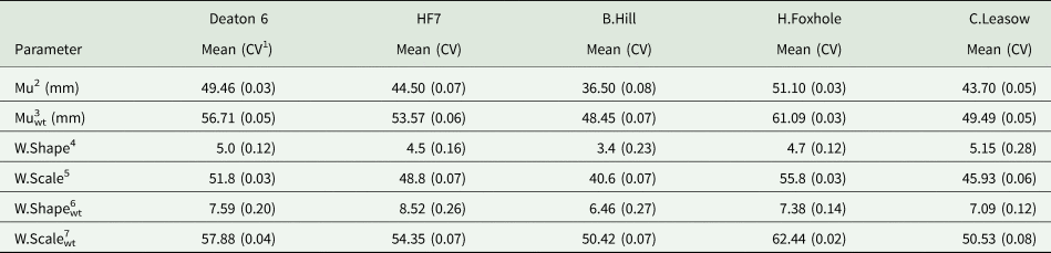
1 = Coefficient of variation. 2 = modal tuber size with respect to proportional tuber weight. 3 = modal tuber size with respect to proportional tuber weight. 4:5 = Weibull or scale shape of proportional tuber numbers. 6:7 = Weibull shape or scale parameter of proportional tuber weight.
Comparison of TSD functions
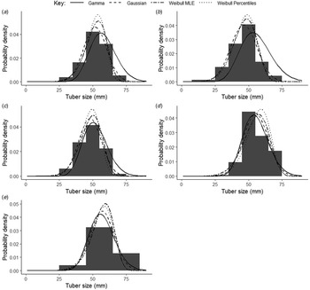
The distribution functions were fitted to the average proportional tuber weights at each location. The Gaussian and Gamma distributions predicted relatively lower probability densities at the modal tuber size compared to the two Weibull distributions (Fig. 2). The Weibull distributions tended to predict higher probability densities between 50 mm and 60 mm but the probability density quickly fell off towards the right tail, predicting low tuber yield in the oversized tuber size fractions (>65 mm). The Gaussian and Gamma distributions decrease towards the right tail and predict higher yields in the oversized fractions.

Fig. 2. The Gaussian, Gamma and Weibull distribution functions fitted to the average proportional tuber weights at HF7 (a), Buttery Hill (b), Crabtree Leasow (c), Deaton 6 (d) and Horse Foxhole (e).
The distribution functions were fitted to the proportional tuber numbers at all five locations (Fig. 3). The Gamma distribution tended to underestimate the TSD relative to the other three fitting methods. Apart from the right-skew at Buttery Hill, the TSD with respect to tuber number was roughly symmetric and the difference between the Gaussian and the two Weibull methods was not readily discernible visually. The Weibull shape at Crabtree Leasow, Buttery Hill, Horse Foxhole and Deaton 6 ranged from 4.7 to 5.0, suggesting left-skewed distribution (Table 3).

Fig. 3. The Gaussian, Gamma and Weibull distribution functions fitted to the average proportional tuber numbers at HF7 (a), Buttery Hill (b), Crabtree Leasow (c), Deaton 6 (d) and Horse Foxhole (e).
The log relative likelihood estimates of the overall distributions of the four tested models, relative to the overall distribution of the observed tuber numbers and tuber weights in each size fraction were calculated (Table 4). The confidence intervals of the estimates are also shown. With respect to tuber number, the Gaussian distribution was found to be the most plausible model at one out of the five locations (Crabtree Leasow) while the Weibull distribution was the most plausible at Branston Booths, Buttery Hill and Deaton 6. The Weibull distribution with percentiles approach to parameter estimation was found to be most plausible at Horse Foxhole, where the tubers were sized in commercially practised main crop size fractions. With respect to tuber weight, the Weibull distribution with MLE was the most plausible model at Branston Booths, Buttery Hill, Crabtree Leasow and Deaton 6, with the highest relative likelihood to the observed discrete distribution as shown in Table 4. Similar to the distributions of the tuber numbers, the Weibull distribution with percentile-based parameter estimation was the most plausible model at Horse Foxhole with no overlapping confidence intervals at all five locations. Overall, the Gamma distribution was found to be the least plausible of the four tested models with respect to both tuber number and weight while the Gaussian distribution ranked second to the Weibull maximum likelihood estimates. The maximum likelihood estimates, particularly the Gamma and Weibull distributions, performed better than the Weibull percentiles approach in generalizing the predicted theoretical curve to the observed discrete distribution, on account of the fitting procedure which took full advantage of the discrete bins in the MLE. On the other hand, when less information (i.e. wider bins) was available as was the case at Horse Foxhole, the Weibull percentiles approach was more plausible than the maximum likelihood approach. While the overall generalization of the distribution to the observed discrete distribution is important, it is more crucial to maximize the log relative likelihood within the marketable tuber size fraction of the main crop (45–65 mm), where the mode of the distribution occurs. This is because the primary goal of modelling TSD is to estimate the tuber size fraction with the highest probability density (Mu). This is used as an estimate of tuber size for the field. Following standard procedures from Travis (Reference Travis1987), the principles of scaling are adopted, such that the weight of an object is proportional to its volume and the volume is in turn proportional to the cubic power of its linear dimensions. Working backwards, the estimated linear dimension (Mu) can therefore be converted to a yield (weight) prediction, incorporating a pre-defined variety-specific tuber shape parameter and observed tuber number. The standard formula for this conversion is provided in Travis et al. (Reference Travis1987). The log relative likelihood of marketable tuber number and weight proportions were calculated (Table 5). With respect to tuber number, the results show that the Weibull percentiles approach generalizes better than all the three other approaches, on account of its high relative likelihood. The closed-form of the percentiles approach meant that the differences between the estimated proportions and the actual proportions were very small, with log relative likelihood approaching zero. For the maximum likelihood approaches, better generalization to the overall distribution as shown in Table 4 meant less goodness of fit in the marketable tuber portion where the mode of the distribution occurs. The same result was observed with respect to tuber weight, where the Weibull percentiles approach performed better that all three other approaches on account of its high log relative likelihood. With respect to both tuber number and weight, the Weibull distribution was also the most plausible of the three models fitted by MLE. This analysis showed that the Weibull distribution with the percentiles approach had the highest log relative likelihood of the observed marketable tuber profile, making it the best candidate for describing the TSD for the purposes of predicting the modal tuber size. However, the maximum likelihood estimate of the Weibull distribution proved to be a better model for generalizing the overall distribution outside the marketable component.
Table 4. Average log relative likelihood estimate and the margin of error (based on 95% confidence interval) of fitted Gaussian, Weibull, Gamma and Weibull Percentiles curves to potato TSDs at five, relative to the likelihood of the observed discrete distribution

1 = Distribution. 2 = Buttery Hill. 3 = Crabtree Leasow. 4 = Horse Foxhole. 5 = Weibull distribution with parameters estimated by MLE. 6 = Weibull distribution with parameters estimated by the percentiles approach.
Table 5. Average log relative likelihood estimate and the margin of error (based on 95% confidence interval) of fitted Gaussian, Weibull, Gamma and Weibull Percentiles curves to the 45–65 mm size band of potato TSDs at five, relative to the likelihood of the observed discrete distribution

1 = Distribution. 2 = Buttery Hill. 3 = Crabtree Leasow. 4 = Horse Foxhole. 5 = Weibull distribution with parameters estimated by MLE. 6 = Weibull distribution with parameters estimated by the percentiles approach.
Using the Weibull distribution with MLE as a benchmark, the deviation of the other models from the benchmark in the prediction of the modal tuber size was as shown in Table 6. With respect to tuber weight, the Weibull percentiles approach yielded the lowest RMSE to the Weibull maximum likelihood approach's mode estimation at all locations except Horse Foxhole. However, as seen in Table 4, the percentiles approach was the most plausible model at Horse Foxhole, therefore its low RMSE approach was considered to be due to the lesser accuracy of the Weibull maximum likelihood approach at this location. These results were mirrored in the RMSEs of the modal tuber weight as shown in Table 6. Apart from Horse foxhole, the RMSE of the shape parameter between the maximum likelihood and percentiles approaches at all locations was within 1.5 units, showing that the percentiles approach approximated the shape of the distribution comparably to the benchmark. Similar observations were made for the scale parameter. At Horse Foxhole, higher RMSEs were observed, partially attributable to the lesser accuracy of the maximum likelihood approach. The analysis showed that the percentiles approach was comparable to the maximum likelihood approach in the estimation of the modal tuber size and yielded the highest log relative likelihood of the observed marketable yield. Therefore the distribution shape, scale and modal tuber size as estimated using the percentiles approach were tested for their predictability using within-field soil nutrient variation.
Table 6. Root Mean Square Error (RMSE) of estimates from the Gaussian, Gamma and Weibull (Percentiles approach) benchmarked against the Weibull model with MLE

1 = RMSE of the mode of Gaussian model vs Weibull MLE, 2 = RMSE of the mode of the Gamma model vs Weibull MLE. 3 = RMSE of mode of the Weibull percentiles model vs Weibull MLE. 4 = RMSE of Weibull percentiles shape vs Weibull MLE. 5 = RMSE of Weibull percentiles scale vs Weibull MLE. 6 = Buttery Hill. 7 = Crabtree Leasow. 8 = Horse Foxhole.
Linear modelling
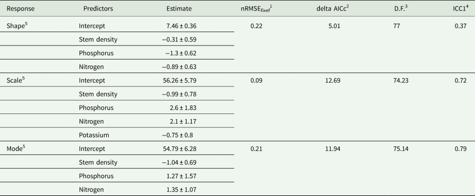
The linear modelling results for the relationships between soil nutrients and TSD parameters with respect to tuber number are presented in Table 7. Stem density was also included as a fixed effect. For the shape parameter, no significant relationship was observed with the stem density. This suggested that the proportional number of tubers falling into the pre-defined size bands was not affected by the stem density. However, P and N were observed to negatively associate with the shape parameter with statistical significance through the confidence intervals (Table 7). The strongest negative relationship with the shape parameter was observed with P, suggesting that P increased the proportional numbers of small-sized tubers. For the scale parameter, a significant negative relationship was observed with stem density, with a standardized regression coefficient of −0.98, suggesting that increased stem densities led to a decrease in the overall range of the distribution. Positive relationships with the scale parameter were observed for P and N, suggesting that the two nutrients increased the overall range of the distribution, though only P was observed to hold a statistically significant relationship.
Table 7. Linear modelling results for the relationships between soil nutrients (and stem density) and TSD parameters with respect to tuber number

1 = Normalized Root Mean Square Error of the fixed effects model, with random effects set to zero. 2 = change in the conditional Akaike Information Criteria between the current model and the random intercept model. 3 = effective degrees of freedom. 4 = Intraclass correlation of the random effects. 5 = parameter determined from the best fitting model.
The overall effect of P on the TSD at the four sites was as shown in Fig. 4, where the average shape and scale parameter from low-P samples (P concentration less than the location mean) and high-P samples (P concentration higher than the location mean) were plotted to visualize the relationship. Overall, an increase in P at all four locations was associated with a shift of the TSD towards a right skew, leading to a lower probability density of the modal tuber size. As shown in Table 7, the mode of the distribution with respect to tuber number was also significantly related to the stem density and P, with a statistically significant regression coefficient of −2.37 for P. Setting the random effects to zero, the fixed-effects-only model had an nRMSE of 0.14 for the mode, suggesting that the expected modal tuber size across the field can be predicted to acceptable accuracy using stem density and soil nutrient information, with a Matern covariance structure fitted across the surface.
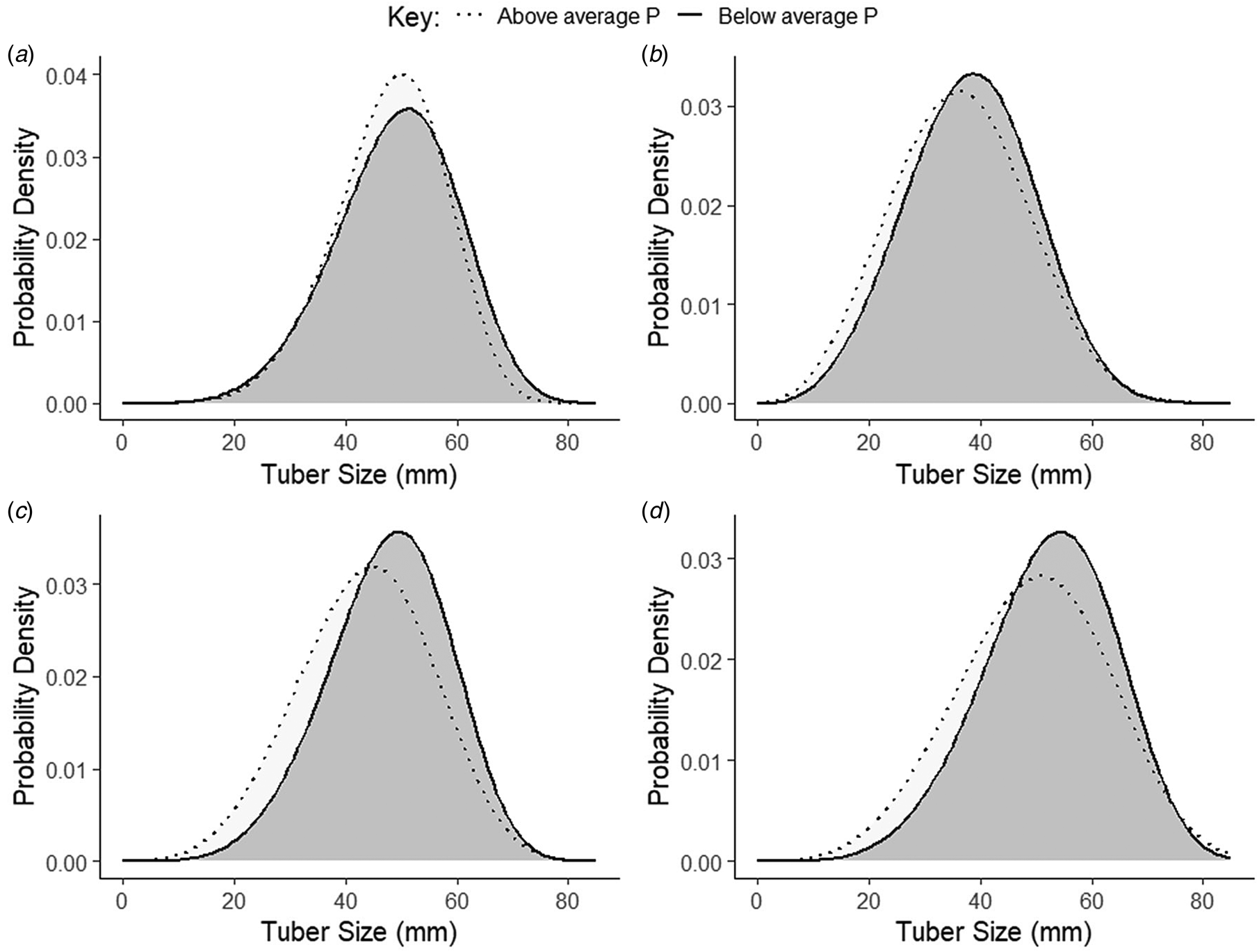
Fig. 4. Illustration of the effect of Phosphorus concentration on the TSD at Deaton 6 (a), Buttery Hill (b), HF7 (c), and Horse Foxhole (d).
The regression coefficients of the shape, scale and mode variables of the TSD (with respect to tuber weight) as a function of stem density and the concentrations of soil nutrients were calculated (Table 8). The shape parameter was negatively related to stem density with a regression coefficient of −0.31, showing that increasing stem numbers moderately associated with a shift of the TSD towards a right skew. The same association was also observed with nutrients P and N, suggesting that increased soil nutrient concentrations in these soils were associated with an increase in the proportion of low-weight tubers. The relationships between the three variables and the shape parameter were all significant as evaluated through their non-zero confidence intervals. The fixed-effects-only model fitted the data with an nRMSE of 0.22. Stem density also had a significant negative association with the scale parameter, which suggested that observations with relatively high stem densities had a smaller range of tuber sizes with a higher concentration of small tubers. Phosphorus and N had significant positive relationships with the scale parameter, suggesting that the overall range of the distribution was increased with the increase of these soil nutrients. Potassium was also negatively related to the scale parameter. The fixed effects explained the variation in the scale parameter with an nRMSE of 0.09. The model fitted for the modal tuber size showed significant negative relationships between stem density and tuber size. Phosphorus and N both had positive relationships with the mode as shown by the positive regression coefficients in Table 8. However, the P relationship was not significant as evaluated the zero-coverage of the confidence interval. The fixed effect coefficients fitted the observed data with an nRMSE of 0.21.
Table 8. Linear modelling results for the relationships between soil nutrients (and stem density) and TSD parameters with respect to tuber weight
1 = Normalized Root Mean Square Error of the fixed effects model, with random effects set to zero. 2 = change in the conditional Akaike Information Criteria between the current model and the random intercept model. 3 = effective degrees of freedom. 4 = Intraclass correlation of the random effects. 5 = parameter determined from the best fitting model.
Discussion
TSD model
The findings of the study showed that potato TSD was more consistent with the Weibull distribution than the Gamma and Gaussian distributions, consistent with Nemecek et al. (Reference Nemecek, Derron, Roth and Fischlin1996) and Bussan et al. (Reference Bussan, Mitchell, Copas and Drilias2007). The log relative likelihood analysis of the overall distribution showed that the maximum likelihood approaches generalized to the observed discrete proportions better than the percentiles approach and the Weibull distribution maximum likelihood approach was the best method for generalizing the shape and scale of the distribution. However, in the context of this study, the percentiles approach performed better at maximizing the likelihood of the tuber size fraction of interest (45–65 mm) because its closed-form offered the opportunity to maintain the likelihood of this desired size fraction accurately. Ultimately, the main goal of TSD modelling is to maximize the likelihood of modelling the correct modal tuber size of a collected sample, which will fall within a pre-defined tuber size interval. In the sample used in this study, the log relative likelihood analysis demonstrated comparable performance between the estimates for the marketable tuber size fraction determined using the Weibull percentiles approach and MLE. Additionally, the Weibull percentiles approach had the lowest RMSE for the prediction of the modal tuber size, in comparison with the MLE approach, while maintaining the highest relative likelihood for the frequency of the marketable 45–65 mm size fraction. Unlike the percentiles approach, the accuracy of the MLE approach can be potentially improved with closer sample-grading intervals. However, closer grading entails more labour at grading time, which affects the adoption of the method in large-scale production environments, making the percentiles approach an attractive option. The relative likelihood for the marketable size range in the MLE method can also be improved by incorporating a weighted approach that provides more weight to the desired size fraction, a trading bias for precision where credible context-specific weight-selection methods can be produced (Hu and Zidek, Reference Hu and Zidek2002). Large variation in the Weibull shape parameter for TSD modelled against both tuber number and weight proportions shows the merit of adopting a flexible distribution function, in contrast to Nemecek et al. (Reference Nemecek, Derron, Roth and Fischlin1996) who suggested an average Weibull shape parameter of 2.3 as a general solution to simulate a right-skewed distribution. However, Nemecek et al. (Reference Nemecek, Derron, Roth and Fischlin1996) used tuber samples from potatoes grown for a seed market, which are desiccated early with less time allowed for tuber bulking. In the current study, a largely right-skewed distribution was observed at Buttery Hill, which also had the smallest average tuber size. The Weibull distribution best modelled the Buttery Hill crop as evidenced by the log relative likelihoods of both the overall distribution and the marketable portion. However, the shape parameter was 3.4 for TSD modelled after proportional tuber numbers and 6.46 for TSD modelled after proportional weight. This showed that proportional tuber numbers were roughly symmetrically distributed around the modal tuber size, but the proportional weights were slightly left-skewed because of a higher weight per tuber of the larger tubers.
Across all locations, the predicted modal tuber size with respect to tuber weight was larger than the modal tuber size with respect to tuber numbers. This is in line with principles of scaling whereby the weight of an object is proportional to its volume, which is in turn proportional to the cubic power of its linear dimensions, the principle behind the use of the modal tuber size for predicting yield in Travis et al. (Reference Travis1987). Therefore, in an assumed Gaussian distribution of tuber numbers, the distribution of tuber weights can be expected to be slightly left-skewed with a higher modal size with respect to proportional tuber weights on account of an exponential increase of weight per tuber with increasing tuber size. These findings provide further evidence that the assumption of a Gaussian distribution as adopted by Travis (Reference Travis1987) does not universally hold true.
Struik et al. (Reference Struik, Vreugdenhil, Haverkort, Bus and Dankert1991) observed an initial right-skewed TSD with a modal tuber size gradually shifting to the right as more time was allowed for tuber bulking by shifting the harvest date. There is good evidence therefore that the overall shape of the distribution is influenced by the average tuber size, which depends on the time of observation, tuber bulking rate and the timing of harvest. It can be argued that the Gaussian (Sands and Regel, Reference Sands and Regel1983), Log-normal (Marshall et al., Reference Marshall, Holwerda and Struik1993) and Gamma (Aliche et al., Reference Aliche, Oortwijn, Theeuwen, Bachem, van Eck, Visser and van der Linden2019) distributions, as well as the Weibull distribution with a fixed shape parameter, are all instance-specific realizations of an underlying dynamic distribution that is a function of the tuber bulking status at the time of observation. In turn, tuber bulking rates are controlled in part by the efficiency of source-sink transportation of photosynthates which depends on the plant nutrition status of the crop (Struik et al., Reference Struik, Vreugdenhil, Haverkort, Bus and Dankert1991). Allowing for a flexible shape parameter, the current results suggest that the Weibull distribution is the best estimator of the TSD curve at any stage of tuber development for the most representative prediction of the modal tuber size, which is the main purpose for modelling TSD.
A method for non-destructively modelling TSD is desirable for temporal monitoring of the changes in TSD. To achieve this, one of the parameters in the Weibull distribution needs to be modelled as a function of a non-destructively measurable variable. Both Nemecek et al. (Reference Nemecek, Derron, Roth and Fischlin1996) and Bussan et al. (Reference Bussan, Mitchell, Copas and Drilias2007) chose to model the scale parameter from empirical data, however, they did so for different reasons. Nemecek et al. (Reference Nemecek, Derron, Roth and Fischlin1996) suggested a fixed Weibull shape parameter, as they empirically observed that distribution fit was relatively invariant in their dataset. However, Bussan et al. (Reference Bussan, Mitchell, Copas and Drilias2007) explicitly modelled the scale parameter because it had a high correlation to measured stem and tuber density. In the current study, the shape parameter had higher within-field variability than the scale at all study sites as measured by the CV, regardless of the method by which TSD was measured (i.e. as a function of proportional tuber number or weight).
Effect of soil factors on the TSD
Literature on TSD is dominated by plant population studies, with the number of stems per unit area being reported to have a negative effect on indicators of TSD and tuber number (Knowles and Knowles, Reference Knowles and Knowles2006; Bussan et al., Reference Bussan, Mitchell, Copas and Drilias2007; Aliche et al., Reference Aliche, Oortwijn, Theeuwen, Bachem, van Eck, Visser and van der Linden2019). These past findings all support the hypothesis that higher stem numbers per unit area increase the tuber number per unit area at the expense of tuber size, leading to more uniform but smaller-sized tubers. The results of the multivariable regression are in general agreement with these findings as stem number per unit area had the most consistent negative regression coefficients with the modal tuber size and the scale parameter of TSD, regardless of whether TSD was modelled with respect to proportional tuber numbers or weight. A lower scale parameter associated with increased stem number means that there was a smaller probability density of large tubers, supporting the previous findings.
The standardized regression coefficients suggest for stem number suggest a large effect size of stem number on the modal tuber size and scale, to provide further support to the hypothesis that stem density increase significantly affects tuber size. Stem density also had consistently negative relationships to the shape of the distribution but the effect size was low, This may be interpreted to mean that bulking rates of large tubers are reduced the presence of high stem numbers but the tuber filling is not altered to particularly favour any one of the other predefined size classes significantly.
The results suggest that the effects of soil macronutrients on TSD may be important, observing negative associations between P and the shape parameter with a high effect size for TSD measured with respect to tuber number or weight. This is consistent with findings that high P tests (25–33 mg/kg) may be associated with an increase in the proportion of small tubers in the TSD, attributed to increased vegetative growth at the expense of tuber bulking (see Birch et al., Reference Birch, Devine, Holmes and Whitear1967; Prummel and Barnau-Sijthoff, Reference Prummel and Barnau-Sijthoff1984; Sharma and Arora, Reference Sharma and Arora1987; Rosen and Bierman, Reference Rosen and Bierman2008).
In the current study, the lowest concentration of available P was observed at Deaton 6 (41 mg/kg), with up to 100 mg/kg at Buttery Hill, which were much greater than the soil P tests at which negative effects were observed in the Rosen and Bierman (Reference Rosen and Bierman2008) study. While positive effects of P on tuber yield components have been reported from replicated experiments by Freeman et al. (Reference Freeman, Franz and de Jong1998), the responses were in low P soils and an asymptote was reached at 27 mg/kg for the Kennebec variety. The results give evidence of a significant negative relationship between P concentrations and the modal tuber size with respect to tuber numbers, meaning that the proportional number of smaller tubers increases as P concentration increases. However, the scale of the distribution with respect to both tuber number and weight was increased with an increase in P concentration. This meant suggests that P did not affect the tuber filling hierarchy but led to the induction of more tubers that remained within the small size fraction. The smaller tubers are expected to have a relatively low contribution to the overall yield therefore the positive effect of P on the scale of the distribution can be expected to positively affect the modal tuber size as observed in the study.
As a possible explanatory mechanism, potatoes are known to maintain P uptake even at high soil P tests like the ones observed in the current study (Jasim et al., Reference Jasim, Sharma, Zaeen, Bali, Buzza and Alyokhin2020), thereby accumulating inorganic P in the cytosol. Inorganic phosphate accumulation is inhibitory to the activity of ADP-glucose pyrophosphorylase and subsequently inhibit the starch synthesis and accumulation in sink organs (Crafts-Brandner, Reference Crafts-Brandner1992; Kleczkowski, Reference Kleczkowski1999; Tiessen et al., Reference Tiessen, Hendriks, Stitt, Branscheid, Gibon, Farré and Geigenberger2002). A tuber-filling hierarchy has been previously shown whereby larger tubers grow the fastest and increase the spread of the TSD (Mackerron et al., Reference Mackerron, Marshall and Jefferies1988), therefore high P concentrations can be expected to contribute to increased proportions of small tuber numbers without penalizing the scale of the distribution as shown in the study.
There have been a few previous studies where the effect of soil nutrients on TSD was systematically studied. Wurr et al. (Reference Wurr, Fellows, Lynn and Allen1993) found that N had a significant effect of TSD measured as the spread (CV %) of tuber sizes (assuming a Gaussian distribution), however, they found no effect of P. The findings by Wurr et al. (Reference Wurr, Fellows, Lynn and Allen1993) are also reflective of the design-intrinsic large concentration gradients of the nutrient treatments in controlled experiments, where N becomes a limiting nutrient hence its effects are emphasized. In the adequately fertilized sites of the current study where N was not a limiting factor for production, the evidence suggests that P equally contributes to the underlying model that explains within-field variation in TSD. Nitrogen was largely found to have the same effects on TSD parameters as P, with positive standardized regression coefficients on the scale and mode with respect to tuber weight suggesting that N increases the variability in tuber size, in alignment with Wurr et al. (Reference Wurr, Fellows, Lynn and Allen1993). High N was associated with a lower shape parameter, showing a particularly high effect size with respect to tuber weight. However, wide confidence intervals call for a more precise estimation of the relationship.
These findings mean that field variation in expected TSD can be constructed from soil data by modelling the shape parameter and scale parameter for the field. The scale and shape parameters can also be calibrated by mid-season yield digs. The beneficial properties of N and P on tuber yield are well documented in the literature and formulate the basis of crop fertilization modelling with the assumption of a Mitscherlich exponential growing process with a horizontal asymptote. The current findings suggest the existence of an inflection point after which over-fertilization results in a linear reduction in the shape of the TSD.
Conclusion
In conclusion, the study has shown that the shape parameter of the Weibull distribution determined using a linearized cumulative probability function provides an adequate index for describing the overall shape of TSD and performs better than the Gaussian and Gamma distributions in simulating observed TSD. The linearized formulae for the Weibull shape and scale presented in the current paper can be easily implemented in spreadsheet software at the farm level. Using the shape parameter, agronomists can improve the monitoring methods of the temporal shift in TSD from yield digs and (where large tubers are preferred) aim for symmetrical (shape ~3) or left-skewed (shape >3) TSD. With the availability of Weibull cumulative probability functions in popular spreadsheet software, tuber numbers in any discrete size grades can be calculated from the modelled shape and scale parameter. From the current study, the shape parameter had larger within-field variability than the scale parameter and was significantly affected by excess P and N. Ultimately, high-intensity soil maps of these elements can enable high-resolution modelling of spatial TSD variation. While requirements for high-intensity soil sampling remain prohibitive, modelling of soil variability using co-kriging proxies like apparent electrical conductivity becomes important and relevant for generating high-resolution field variation for decision-support. Subsequent studies to validate these findings in more environments are recommended, as well as controlled studies to investigate the general point of inflection at which additional fertilization becomes detrimental to TSD.
Acknowledgements
Acknowledgement to the Crops and Environment Research Centre of Harper Adams University and Branston Limited for providing the experimental sites for this study. Many thanks to William Johnson, Andrew Beacham, Kevin Jones, Gary Weston, Grace Milburn and Joseph Crosby for their technical help.
Financial support
This work was supported by the Agriculture and Horticulture Development Board (Stoneleigh Park, Kenilworth, Warwickshire, CV8 2TL, United Kingdom) [Project Number 11140054].
Conflicts of interest
The authors declare there are no conflicts of interest.
Ethical standards
Not applicable.


 Open access