


NOMENCLATURE
- AR
aspect ratio, b2/S
- a
similarity variable, α/tan(ε)
- b
wingspan
- C D
drag coefficient
- C D,o
minimum drag coefficient ΔC D.C D − C D,o
- C L
lift coefficient
- C Lα
lift curve slope
- C L,p
potential flow lift coefficient
- C L,v
vortex flow lift coefficient
- C m
pitching moment coefficient
- C p
pressure coefficient
- ΔC p
lifting pressure coefficient, Cp,1 – Cp,u
- c
wing chord
- c n
section normal force coefficient
- c r
root chord
- c s
section suction coefficient
- c t
tip chord
- cref
reference chord
- F
force vector
- K p
constant, potential-flow
- K v
constant, vortex flow
- M
Mach number. Also, million
- mac
mean aerodynamic chord
- P t
total pressure
- Re c
Reynolds number based on wing chord, U∞ c/v
- r
radial direction, also radius
- S
wing area, also entropy
- s
local semi-span
- U ∞
free stream reference velocity
- x,y,z
body-axis Cartesian coordinates
- α
angle-of-attack, deg.
- β
sideslip angle, deg. Also, Prandtl-Glauert factor,
 \[{(M_\infty ^2 - 1)^{1/2}}\]
- ε
delta wing semi-apex angle, deg.
- ξ
inner-law radial coordinate
- θ
circumferential coordinate
- Λ
sweep angle, deg.
- λ
taper ratio, ct/cr
- μ
viscosity
- v
kinematic viscosity, μ/ρ
- ρ
density
- ϕ
perturbation velocity potential
- ψ
radial distance
- e
edge
- inc
increment
- l
lower surface
- le
leading edge
- max
maximum
- min
minimum
- p
potential flow
- te
trailing edge
- u
upper surface
- v
vortex flow
- vc
vortex core
- ∞
freestream reference condition
- AGARD
Advisory Group for Aeronautical Research and Development
- AIAA
American Institute of Aeronautics and Astronautics
- AMR
Adaptive Mesh Refinement
- ASME
American Society of Mechanical Engineers
- CAWAP
Cranked Arrow Wing Aerodynamics Program
- CFD
Computational Fluid Dynamics
- DES
Detached Eddy Simulation
- DLR
German Aerospace Centre, Germany
- DNS
Direct Numerical Simulation
- EADS
European Aeronautic Defence and Space Company, Germany
- FC
Flight Condition
- FVS
Free Vortex Sheet
- LaRC
Langley Research Center
- LES
Large Eddy Simulation
- LEX
Leading-edge Extension
- LMAL
Langley Memorial Aeronautical Laboratory
- NACA
National Advisory Committee for Aeronautics
- NASA
National Aeronautics and Space Administration
- NATO
North Atlantic Treaty Organization
- RAE
Royal Aircraft Establishment, UK
- NTF
National Transonic Facility
- ONERA
French Aerospace Laboratory, France
- RANS
Reynolds-Averaged Navier-Stokes
- RTO
Research and Technology Organization
- SA
Spalart-Allmaras turbulence model
- STO
Science and Technology Organization
- TUM
Technische Universität München, Germany
1.0 INTRODUCTION
High-speed aircraft often develop separation-induced vortices in various portions of their flight envelope. Through interactions with the airframe, these separation-induced vortices affect the overall vehicle performance and stability and control in ways that can either be favourable or adverse. These overall effects can be referred to as vortex flow aerodynamics. Prediction of the airframe aerodynamics with separation-induced vortices has been anchored in experimental aerodynamics, although theoretical modelling along with more recent numerical simulations has greatly expanded our understanding of these vortical flows. Although the application of vortex flow aerodynamics is most commonly associated with manoeuvring military vehicles, it applies to a much broader class of vehicles and flow applications.
In this article, a review is presented of the experimental discovery of separation-induced edge vortices and the subsequent evolution of theoretical and numerical prediction techniques for vortex flow aerodynamics. A brief discussion is first presented to define vortex flow aerodynamics and establish the particular focus for the article, separation-induced leading-edge vortices. Next, several experimental activities that led to the discovery and initial understanding of separation-induced vortices on wings and their consequences for wing aerodynamics are reviewed. This is followed by the evolution of physics-based theoretical modelling of these vortices as well as the subsequent evolution of vortex capturing methods along with application assessments for the prediction of vortex flow aerodynamics. Finally, a capability assessment for numerically predicting separation-induced leading-edge vortices and their subsequent aerodynamic effects is summarised.
Aerodynamic predictions can be accomplished by experimental, theoretical or numerical means. The predictive portion of this paper will focus only on the latter two. There have been extensive experimental prediction programs of vortex flows, both for fundamental understanding as well as for airframe performance, and proper treatment of the scope of this work would require a separate publication. One summary has been given by Squire(Reference Squire1) in 1981. However, experiments generally provide guidance to theoretical and numerical predictive method development and select experiments that helped guide this development are included. In addition, this author has selected highlights to illustrate the evolution of methods, and it is recognised that many others are available.
This article grew from the 2017 F. W. Lanchester lecture. The author has chosen to first review a few details of Lanchester’s contributions to aeronautics and the context for these contributions.
2.0 LANCHESTER BACKGROUND
Frederick W. Lanchester was born in October 1868 and lived until March 1946. Lanchester’s professional career began in the early 1890s, and his interests were divided between aircraft and ground-based locomotion. The majority of his career was spent on the latter, and he held many patents for his inventions that contributed significantly to the creation of cars, trucks, tanks and even motorboats.
Lanchester’s aeronautics studies began in 1892 and were sustained roughly through 1918. This was a pioneering era for aeronautics. For perspective, we recall that the Wright brothers invented the airplane(Reference Gibbs-Smith2) with their first powered flight in December of 1903, Prandtl(Reference Prandtl3) published his boundary layer concept in 1904, Prandtl(Reference Prandtl4) published his lifting-line theory in 1918 and Munk(Reference Munk5) published his dissertation with the minimum-induced drag concept in 1918. Many things taken for granted amongst the contemporary aeronautics community were only being discovered during Lanchester’s time. A photograph of Lanchester from the era of his aeronautics research is provided in Fig. 1.
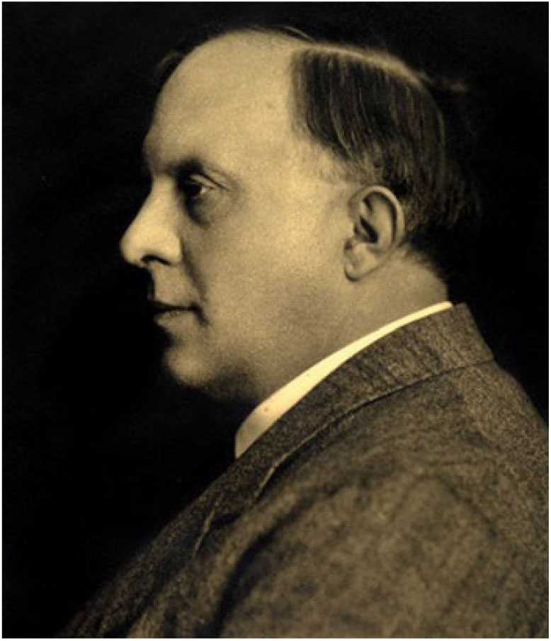
Figure 1. Frederick W. Lanchester, circa 1910.
Lanchester appears to have been a polymath. His methods of research included observing nature, conceiving and executing his own physical experiments and developing mathematically-based theoretical interpretations of his observations. He published books as well as conceived, designed, built and patented many practical devices.

Figure 2. Lifting wing properties, Lanchester(Reference Lanchester7), Figs. 79 and 86. (a) Tip vortex. (b) Trailing vorticity coalescence.
Lanchester is credited with developing the theory of circulation during the years 1892–1897, having performed his own experiments, and wrote a paper in 1894 (see, von Karman(Reference Von Karman6)) that was presentedFootnote 2 that same year. This work was offered to the Physical Society of London in 1897 but, unfortunately, was never published. Lanchester continued his aeronautics research, which led to three significant books. The first book(Reference Lanchester7) was published in 1907 and addressed aerodynamics. In this book, Lanchester had developed the relationship between circulation and lift for a wing and understood the connection between spanwise variation of lift and the development of a vortex wake. Von Karman(Reference Von Karman6) reported that Lanchester was the first to address lift on a wing of a finite span, developed the concepts of a bound wing vortex connected to trailing free vortices from the wing tip and understood the significance of aspect ratio on wing performance. Figure 2 illustrates some of his concepts and shows how circulation from the wing sheds into a tip vortex as well as how the trailing wake vorticity coalesces into a trailing vortex. Lanchester’s second book(Reference Lanchester8) was published in 1908 and addressed flight mechanics. In this book, he developed the phugoid theory of motion. His third book(Reference Lanchester9) was published in 1916 and addressed the use of aircraft in warfare. In this book, he developed differential equations to model the outcome of aerial combat accounting for differences in strength between the opposing forces. This led to what became known as the Lanchester Power Laws, and Lanchester is credited as a co-inventor of what later became known as Operations Research (OR).
Much of Lanchester’s aeronautics work appears to have been not fully appreciated during the time of its creation. Throughout the era of his aeronautics research, he was encouraged to be more practical, and he continued his research and development of ground-based transportation while performing his aeronautics work.
3.0 VORTEX FLOW AERODYNAMICS
Vortex flow aerodynamics will refer to the focused and direct interaction of a concentrated vortex with an aircraft component at any scale with a direct consequence to the vehicle’s aerodynamic performance. This definition includes many vortical flows from the aircraft but will exclude the wing wake that rolls up as a consequence of the spanwise variation of lift. The vortices, in general, are initiated by flow separation after which they interact with the vehicle components.
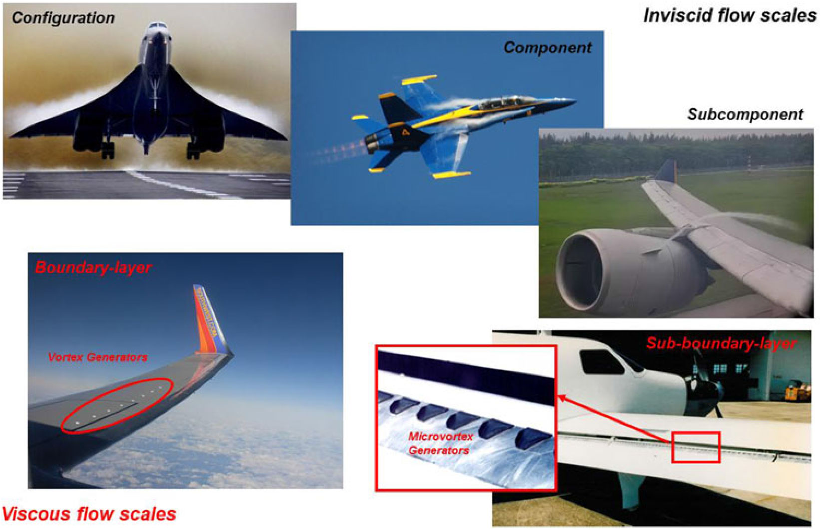
Figure 3. Multiple scales for vortex flow aerodynamics.
Vortices that produce vortex flow aerodynamics can occur over a broad range of scales, and some examples are shown in Fig. 3. The upper portion of the figure illustrates vortices that occur at inviscid flow scales. The examples include vortices that are manifested on a full configuration scale (the wing of a supersonic transport), a component scale (the leading-edge extension of a fighter aircraft) or a subcomponent scale (a strake added to the engine nacelle of a commercial transport). The lower portion of the figure illustrates separation-induced vortices that occur at viscous flow scales. Vortex generators reside in the boundary layer and generate vortices near its edge, and an example is shown for the wing of a commercial transport. Microvortex generators(Reference Lin, Robinson, McGhee and Valarezo10, Reference Lin11) are designed to generate vortices within the boundary layer, and here an example is shown on the flap of a general-aviation aircraft. In all of these examples, the vortices are induced by separation along an edge. These applications that are now considered in many ways routine and fairly well understood were all but unknown during Lanchester’s time.
The focus for this paper is on separation-induced leading-edge vortices at the configuration and component scales. For this focus, the configurations generally have been designed with high-speed (supersonic) capability resulting in thin and highly swept wings and components. The leading edges for these wings will have small leading-edge radii and, in some applications, will be sharp. Some separation-induced vortices from forebodies will also be included. The discovery of these separation-induced leading-edge vortices, and their subsequent use for vortex flow aerodynamics, is anchored in the development of high-speed military aircraft. This will be discussed in the next section.
4.0 DISCOVERY OF VORTEX FLOW AERODYNAMICS
Vortex flow aerodynamics has its origins in a design revolution for high-speed military aircraft that occurred following World War II, Fig. 4. At the end of this war, the North American Aviation (NAA) P-51 Mustang was indicative of a state-of-the-art fighter aircraftFootnote 3 and remained in active front-line service into the early 1950s. In very little time, the Convair YF-102A Delta Dart had been successfully developed. Whereas the P-51 maximum speed was Mach 0.625, the YF-102A achieved Mach 1.25; the era of the supersonic fighter aircraft had arrived. Amongst a number of revolutionary features was the thin and highly swept delta wing, which introduced many new aerodynamic challenges.

Figure 4. Design revolution for high-speed military aircraft. (a) P-51, circa 1944. (b) YF-102A, circa 1953.
Figure 5. Effect of Aspect Ratio on low-speed attached-flow lift-curve slope.
One critical challenge for the delta-wing aircraft was the greatly diminished low-speed lift-curve slope due to aspect ratio effects. An example of this effect is shown in Fig. 5. The figure includes the low-aspect-ratio bound from Jones(Reference Jones12) slender-wing theory and the high-aspect-ratio bound from flat-plate aerofoil theory. For finite aspect ratio wings, a theory due to Polhamus(Reference Polhamus13) is shown that accounts for both sweep and taper as well as aerofoil section. The examples include both delta wings and unswept wings with a National Advisory Committee for Aeronautics (NACA) 0012 aerofoil section along with experimental values. The Polhamus theory provides a useful approximation to the measurements and helps demonstrate the reduction in lift-curve slope that could be anticipated in changes from the nominally AR = 6 P-51 class aircraft to a nominally AR = 2 delta-wing aircraft. The lift-curve slope is cut in half; thus, take-off and landing performance could require significantly higher speeds and/or angles of attack. This, of course, assumes the same flow physics for both wings, and the discovery of separation-induced leading-edge vortex flows helped resolve this issue.
The revolutionary design change from the unswept tapered wing, such as from the P-51 in 1944, to the thin and highly-swept delta wing, such as from the YF-102A in 1953Footnote 4, was enabled in part by the experimental discovery of separation-induced leading-edge vortex flows and their subsequent aerodynamic properties for the thin and highly-swept delta wings. Before proceeding with a summary of these vortical discoveries, a brief mention is warranted for two other experimental configuration development programs that preceded this work and related to delta-wings.
Between 1931 and 1939, Lippisch(Reference Lippisch14) developed a series of five tail-less aircraft that he called delta wings. The aircraft incorporated swept and tapered wings, with thick aerofoil sections and were advanced for their time. However, these were not delta-wing aircraft in the sense the term is used today for aircraft whose design includes supersonic flight considerations. Lippisch’s series of swept/tapered configurations enabled higher-speed subsonic flight than contemporary configurations with unswept wings and contributed to the development of the Messerschmitt ME-163 Komet.
Payen(Reference Lepage15) developed an unorthodox tandem-wing aircraft between 1935 and 1939. The aircraft incorporated an essentially unswept forward wing of moderate aspect ratio and a highly swept aft delta wing that was thin and had 67° leading-edge sweep. This French experimental aircraft was confiscated by Germany, and the first flight of the Payen PA-22 occurred in October 1942. To this author’s knowledge, this is the first delta-wing aircraft flown, but no documentation of vortical flows on the Payen PA-22 has been found at of the time of this writing.
The discovery of separation-induced vortex flows from low-aspect-ratio wings was anchored in additional German research that was fundamental in nature. Its exploitation for what became slender-wing vortex flow aerodynamics was anchored in American research with an advanced German prototype aircraft, also developed by Lippisch. Some details from this research of the original observation and description of a separation-induced vortex flow from a lifting wing along with the subsequent rediscovery and exploitation for what became vortex flow aerodynamics are reviewed in the next two sections.
4.1 Separation-induced vortex flow, flat plates
The earliest discussion of a separation-induced vortex from a lifting wing edge was given by Winter(Reference Winter16) in 1935. This work was directed at measuring aerodynamic properties of low aspect ratio plates. Configurations included flat plates that were rectangular, triangular, elliptic and semi-elliptic with asymmetrically bevelled sharp edges. A circular planform was also included. Some of the rectangular planforms were also tested with aerofoil sections. Aspect ratio varied between 0.033 and 2 amongst these planforms. Low-speed wind-tunnel measurements included force and moment coefficients, surface pressures and flow visualisation. Drag polar and pitching moment data were reported for all planforms; normal force data were included only for the rectangular flat plates, and pressure data were reported for one of the rectangular flat plates.

Figure 6. Side-edge vortex flow, rectangular plates. Winter(Reference Winter16). (a) Side view of side-edge vortex.AR = 0.033. M:0, α = 16°. (b) Postulated spanwise lift distributions, AR = 0.5.
Winter’s critical analysis was for the side-edge vortex from his rectangular flat-plate wings, and two of Winter’s figures, with this author’s annotation, are reproduced in Fig. 6. Most of Winter’s analysis was based upon his flow-visualisation measurements, and he identified the rolled-up vortex at the side edge of his flat AR = 1 rectangular plate. At a lower aspect ratio (Fig. 6(a)), Winter identified the core of the side-edge vortex and attributed the break in trajectory due to the vortex diameter becoming large as compared to the wing semi-span, an effect referred to today as vortex crowding. From his surface oil-flow visualisation, Winter discussed the reattachment of flow induced by the vortex and the suction-surface streamline pattern of flow moving away on both sides from the reattachment line. Additional analysis was included for a vortical separation that forms from the unswept leading edge.
The NACA translation in Ref. Reference Winter16 contains some additional information from Winter’s thesis, and in this work, Winter postulated the effect of the side-edge vortex pressures on the spanwise distribution of lift, Fig. 6(b). In this sketch, the wing is viewed from downstream, and an indication of the attached flow about the side edges is shown. Winter showed three spanwise distributions of lift: (i) two-dimensional flow, (ii) three-dimensional attached wing flow and (iii) three-dimensional wing flow with side-edge vortices. His sketch clearly shows the induced effect of the side-edge vortices on the lift distribution. Winter further proposed that the high values of CL,max from his measurements were due to the effects of these side-edge vortices. Winter also observed that the edge vortices formed on his elliptic planform wing included some of the leading edge near the wing tip, which contributed to the high lift of this as well as other configurations tested.
Winter’s description of the side-edge vortex appears to have introduced, for the first time, a number of fundamental properties of what we would now call a separation-induced side-edge vortex on a lifting wing (although for the most part these were only flat rectangular plates). The extent to which his results were used for contemporary wings is unclear. During the 1930s, the advantages of jet propulsion had been recognised, and by the late 1930s, several countries had operating versions (Polhamus(Reference Polhamus17)). High-speed wing design lagged somewhat behind, although a number of advanced concepts had been demonstrated in Germany with aircraft in various stages of development. One example was the Messerschmitt ME-262, which successfully incorporated jet propulsion in conjunction with the swept wing concept. Another example was a prototype delta-wing aircraft that led to the realisation of vortex flow aerodynamics. This is the topic for the next section.
4.2 Separation-induced leading-edge vortex lift, delta-wing aerodynamics
The benefits of sweep had remained a mystery outside of Germany until theoretical analysis was developed by Jones(Reference Jones18) in 1945. This work demonstrated the benefit of sweeping the wing aft of the Mach cone for supersonic flight. Also, Jones’s results explained the benefits of sweep for subsonic speeds, independent of Busemann’s(Reference Busemann19) studies a decade earlier. Combined with Jones’s(Reference Jones12) contemporary slender-wing work as well as with other studies, the Allied countries were beginning to understand the benefits of sweep. The thin delta wing, combined with jet propulsion, had been identified as a fighter-aircraft concept that offered promise for supersonic flight capability.
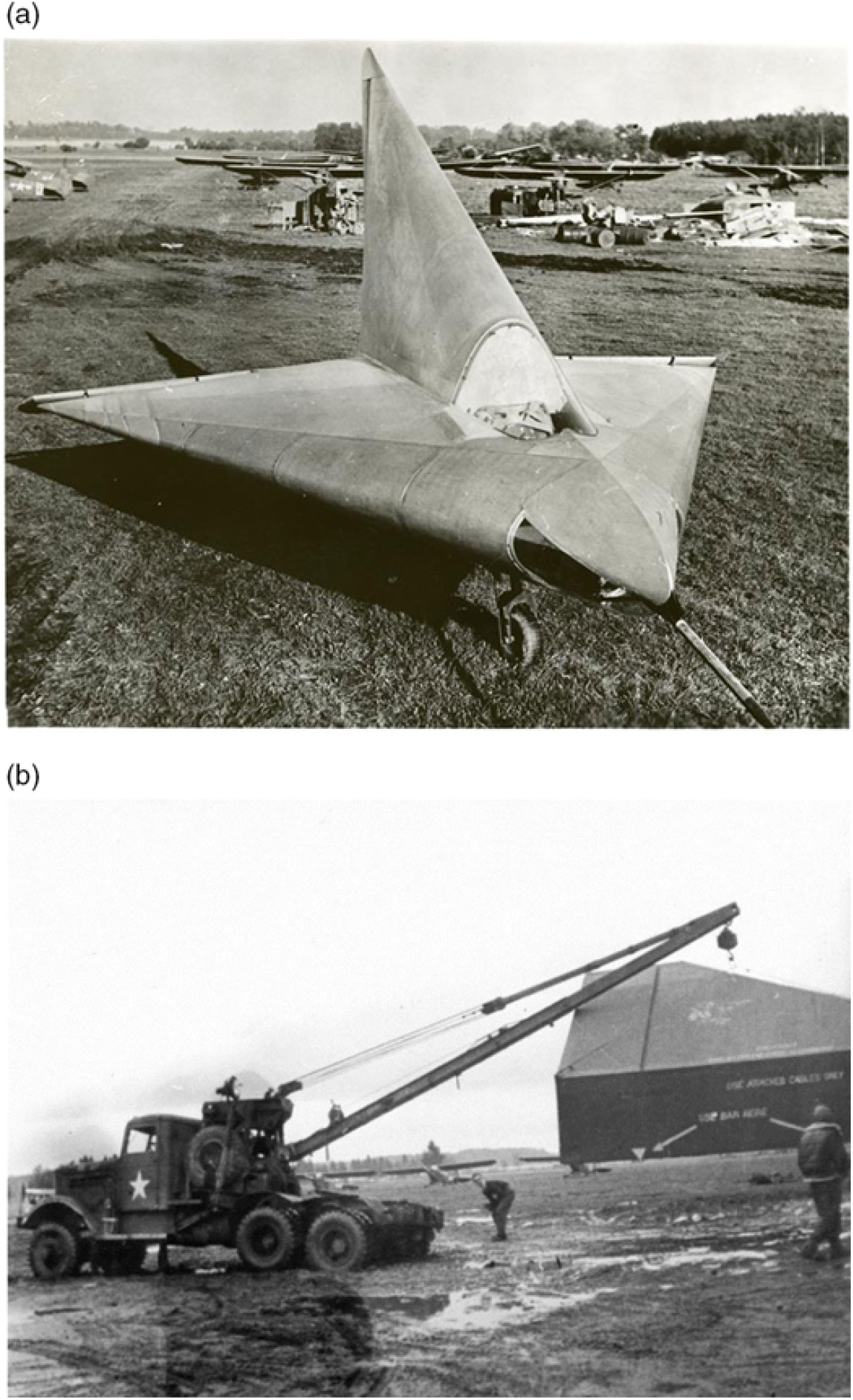
Figure 7. Lippisch DM-1 glider, 1945. (a) DM-1 vehicle. (b) Shipment to NACA Langley.
At nearly the same time, an unusual full-scale delta-wing configuration, developed by Dr. Alexander Lippisch, had been discovered at the discovered at the Prien am Chiemsee airbase in south-eastern Germany in the spring of 1945 just as World War II was ending (Fig. 7). This configuration was one of a series of prototype vehicles envisioned by Lippisch to enable supersonic, and possibly hypersonic, flight. This particular vehicle was intended to explore low-speed performance and handling properties as a glider and was still under fabrication at the time of its discovery by Allied forces. The vehicle was known as the Darmstadt-München-1 (DM-1), and the United States (US) government decided to study the low-speed aerodynamics of this most unusual configuration. The DM-1 was shipped to NACA Langley for testing in the Langley Memorial Aeronautical Laboratory (LMAL) 30-by-60ft Full-Scale Tunnel, and a photograph of the DM-1 in this facility is shown in Fig. 8. The tests were performed in 1946 and reported by Wilson and Lovell(Reference Wilson and Lovell20).
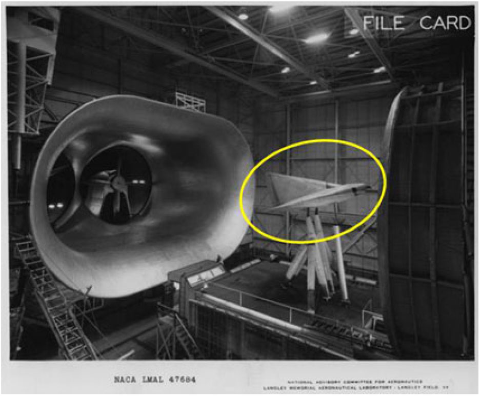
Figure 8. DM-1 glider test in LMAL 30- by 60-Foot Full-Scale Tunnel, 1946.
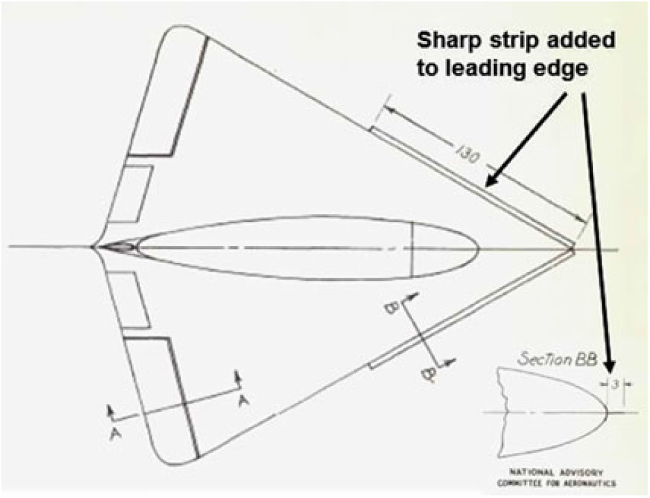
Figure 9. Drawing of DM-1 glider with sharp leading-edge strip. Wilson and Lovell(Reference Wilson and Lovell20).
The DM-1 differed from the high-speed delta wing planning of that time in that it was thick and had very blunt leading edges. Initial test results for the full-scale vehicle showed an unanticipated low angle-of-attack for wing stall, with a corresponding low maximum lift coefficient. Earlier tests of subscale models had not shown this feature, and subsequent testing of a new subscale model of the DM-1 revealed a laminar separation at the leading edge, with subsequent vortical flow over the wing. At the low Reynolds numbers of these subscale tests, this flow produced high lift coefficients at high angles of attack. It was then reasoned that a sharp leading edge could force the leading-edge vortex flow to occur, even at the high Reynolds numbers of the full-scale DM-1 vehicle. The DM-1 was modified to incorporate a sharp leading-edge strip, as shown in Fig. 9, and the subsequent testing produced large lift increments, compared to the clean configuration, due to the formation of the separation-induced leading-edge vortices over the wing. An example of the forces and moments from the Wilson and Lovell report is shown in Fig. 10(a). Wilson and Lovell attributed the lift increments to the formation of leading-edge vortices, and a second figure from their report with this interpretation is reproduced in Fig. 10(b). Dr. Samuel Katzoff of NACA Langley contributed to the early and qualitative interpretations of these vortical flows, and Wilson and Lovell cited similarities between their leading-edge vortex flows and the side-edge vortex flows reported earlier by Winter(Reference Winter16).

Figure 10. DM-1 results. Wilson and Lovell(Reference Wilson and Lovell20). (a) Forces and moments. (b) Flowfield interpretations.
The Wilson and Lovell results clearly established the connection between the high angle-of-attack lift increments and leading-edge vortex flows for the DM-1. Their work also established the role of leading-edge bluntness in a context of Reynolds number effects for the leading-edge separation.
Winter had established some basic flow features of a separation-induced side-edge vortex along with its contributions to the aerodynamics of a series of flat-plate planforms. One could argue that Wilson and Lovell extended this work to separation-induced leading-edge vortex flows with a view towards the configuration aerodynamics of a more complex aircraft concept. By forcing the leading-edge vortex to form on the DM-1 configuration, Wilson and Lovell had a clear indication of the vortex-lift increment due to the separation-induced leading-edge vortex. However, this work and report remained classified for some time and was only shared amongst US industry and government laboratories; it was not known outside of the US to the broader slender-wing community that was developing. Some additional details of the experiments have been given by Chambers(Reference Chambers21), and additional comments on this discovery of vortex lift for the modified DM-1 configuration have been given by Polhamus(Reference Polhamus17).
The modified DM-1 was the first aircraft concept to exhibit separation-induced leading-edge vortex flows and to use what we now would call vortex flow aerodynamics to resolve a particular performance issue. These vortex flows could now be studied experimentally in the course of developing the new generation of slender-wing aircraft. There was close collaboration between NACA and US industry, which included Convair where Lippisch now worked. The DM-1 was modified at NACA Langley to better represent a prototype aircraft configuration. These modifications included an integral sharp leading edge, a more typical bubble canopy and a reduced vertical tail. Wind-tunnel testing of this modified DM-1 in the LMAL 30-by-60-foot Full-Scale Tunnel is shown in Fig. 11(a).
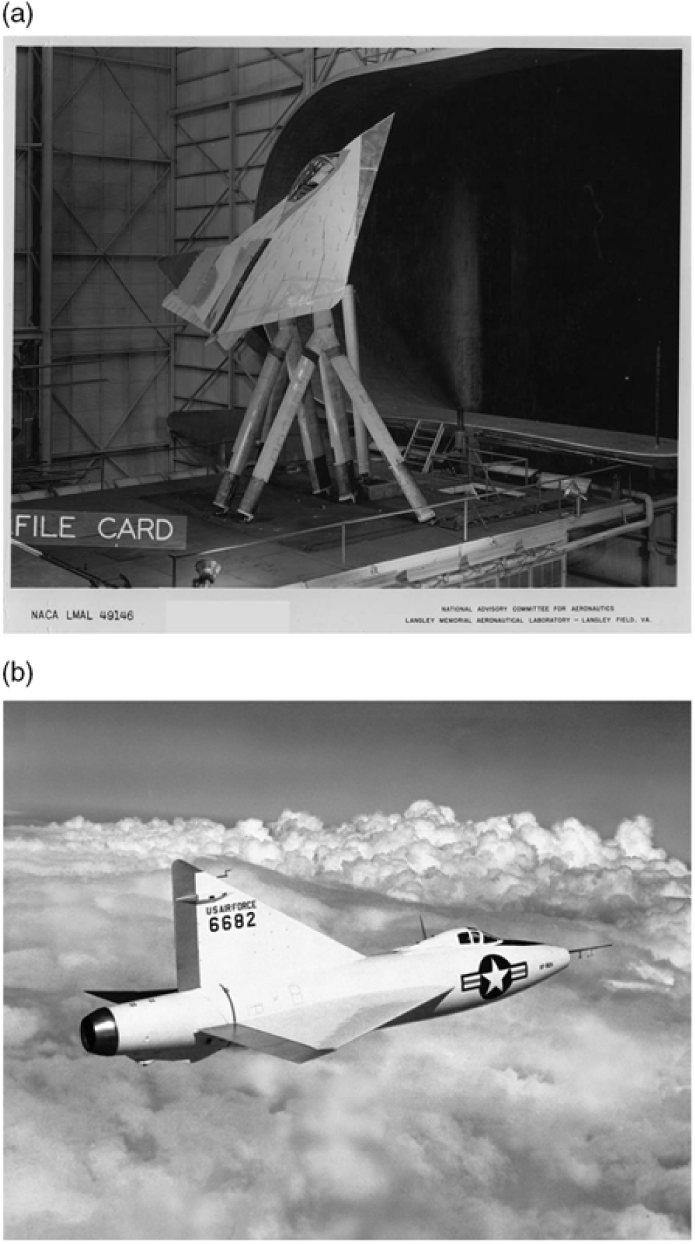
Figure 11. Evolution from the DM-1 to the Convair XF-92A aircraft. (a) Modified DM-1 (b) XF-92A.
Further configuration advancements were developed by Convair, and these included a stretched fuselage to accommodate a jet engine, a thin wing and other systems required for an experimental aircraft. This led to the creation of the experimental XF-92A aircraft, Fig. 11(b). The first flight for the XF-92A was in September of 1948, and this was the first jet-powered delta-wing aircraft to fly(22). Flight tests subsequently demonstrated supersonic flight (albeit in a dive) and controlled low-speed flight up to 45° angle-of-attack. The controlled high angle-of-attack performance reduced landing speed from a predicted 160 miles per hour to only 67mph. The separation-induced leading-edge vortex flows were found to provide exceptional low-speed high angle-of-attack flight capability for this experimental delta-wing aircraft. Other benefits of separation-induced leading-edge vortex flows have been summarised by Polhamus(Reference Polhamus23).
The XF-92A remained an experimental aircraft only, as configuration designs had already evolved experimentally beyond this particular vehicle. Experimentation was relied upon for developing configuration aerodynamics, and now this grew to include prediction of vortex flow aerodynamics. However, there were no theories to predict the high angle-of-attack vortex flow aerodynamics, and this led to an evolution of theoretical methods. The methods were focused on physics-based modelling of the leading-edge vortices in proximity of the lifting wing. The methods began with simplified models, which grew incrementally to include more physics of the subject vortex flows. Later, this work switched from modelling to capturing the vortices with Computational Fluid Dynamics (CFD) numerical techniques. This evolution will be discussed in the next section beginning with a review of some fundamental vortex flow physics that affect slender-wing aerodynamics. Although the original motivation for these studies came from a military aircraft perspective, a second motivation arose in the 1960s for the development of a supersonic commercial transport that, in Europe, led to the creation of the Concorde.
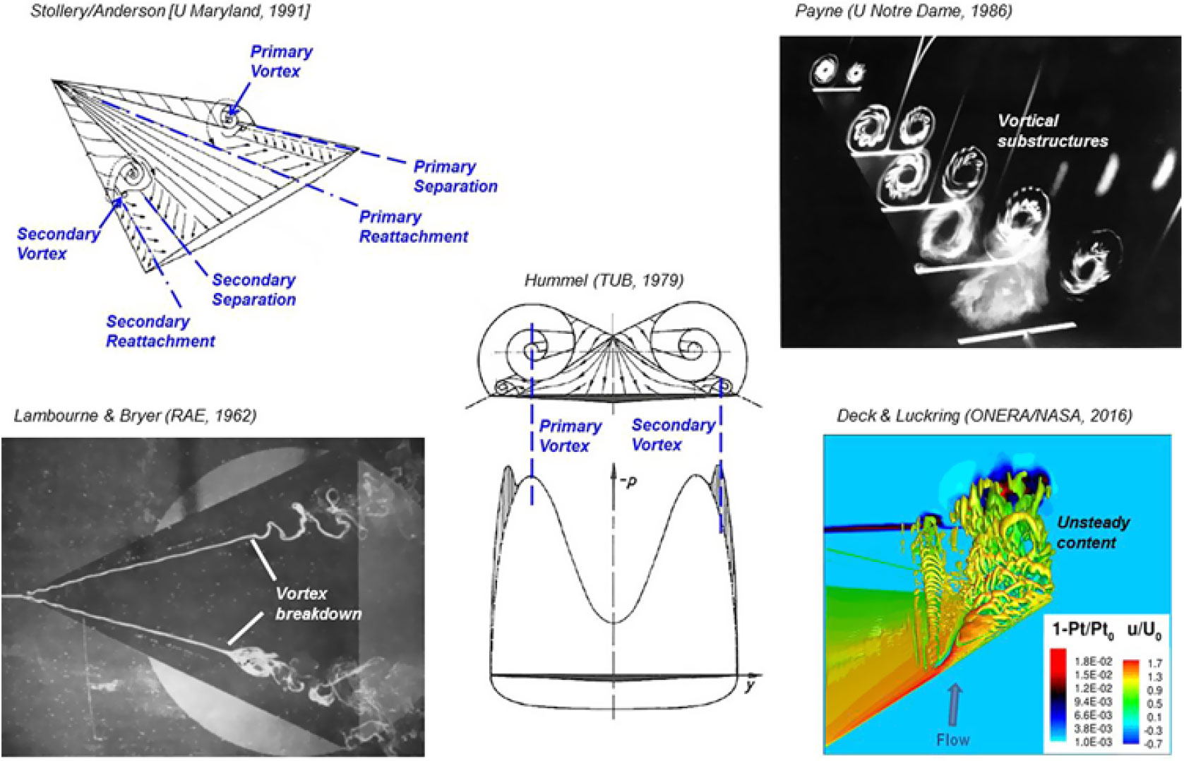
Figure 12. Leading-edge vortex flow physics.
5.0 PHYSICS-BASED THEORETICAL MODELING
The fundamental low-speed physics of a separation-induced leading-edge vortex flow can be reviewed using a highly swept sharp-leading-edge delta wing, and examples are shown in Fig. 12. The upper-left image (Anderson(Reference Anderson24)) illustrates the primary leading-edge vortex with primary separation at the sharp leading edge and induced primary reattachment inboard on the upper surface of the wing. Spanwise flow is induced under the primary vortex. This flow separates from the smooth upper surface along a secondary separation line to form a counter-rotating secondary vortex. The secondary vortex is also shown in the sketch by Hummel(Reference Hummel25) along with wing suction pressures due to the vortices. The primary vortex sheet itself can form vortical substructures, an example of which is shown in the upper right portion of Fig. 12 from Payne(Reference Payne, Ng, Nelson and Schiff26).
The primary vortex sheet rolls up upon itself to form a vortex core. At the centre of the core, the flow has become aligned with the axis of the vortex, and a new phenomenon known as vortex breakdown can occur. An example is shown in the lower-left portion of Fig. 12 from Lambourne and Bryer(Reference Lambourne and Bryer27). Multiple modes of bursting can occur, and the image shows both the bubble and spiral modes of vortex breakdown. Vortex breakdown is a locally unsteady phenomenon, and unsteady effects can also occur in the vortex sheet as illustrated in the lower-right portion of Fig. 12 from a contemporary treatment by Deck and Luckring(Reference Deck and Luckring28) for a diamond wing. Other unsteady effects can occur and have been summarised by Gursul(Reference Gursul, Gordnier and Visbal29). Even for the simple, sharp-edged delta wing, the separation-induced leading-edge vortex system contains many complex flow features. The vortices fundamentally alter the delta wing aerodynamics from what would be realised for an attached flow.
The first theoretical models for the prediction of vortex flow aerodynamics were developed by exploiting reductions in flow complexity. This took the form of both reduced dimensionality as well as reduced physical complexity of the vortical models. Thus, this allowed the remaining vortex physics to be analysed with established mathematical methods that were augmented with some numerical solution techniques. As knowledge and numerical capacity grew, additional vortex physics were modelled with the side benefit that incremental effects resulting from the additional physical modelling could be observed.
The time span for these vortical studies includes several paradigm shifts in vortex modelling, to a large degree due to the advent and development of scientific computing. Both evolutionary and revolutionary developments were demonstrated. Early work required explicit modelling techniques for the vortices, whereas later work focused on flow solvers that could implicitly capture vortical flows. This was perhaps the largest paradigm shift for the theoretical/computational studies of slender-wing vortex flows.
Theoretical models will be presented in their chronological order of development, which also results in a successive complexity increase in the vortical models. Many of these models assumed steady flow. The first section will address modelling of a single steady vortex generated from a sharp leading edge in reduced dimensions. The second section will address modelling of a single steady vortex generated from a sharp leading edge for three-dimensional flow. The third section will address modelling of vortices generated from a blunt leading edge, and the final section will address vortex interactions of several types for three-dimensional flows. This last section includes some unsteady effects as well.
5.1 Reduced dimensions, sharp edge, 1 vortex
A baseline for the theoretical predictions of slender-wing aerodynamics was first established for attached flow by Jones(Reference Jones12) in 1946. Small disturbance assumptions had already been developed for the analysis of two-dimensional aerofoil flows and could be applied to wings with a large span and relatively small chord. Jones used similar assumptions for the theoretical analysis of wings at the other extreme condition i.e., wings with a small span and large chord. An example is shown in Fig. 13 for a delta wing of infinite extent. The resultant flow is conical, with properties being constant along rays emanating from the wing apex, and solutions were obtained with the Jones theory through crossflow plane (x = const) analysis.
Jones’s solutions demonstrated that the lift is proportional to the growth of the wing semi-span in the downstream direction, tan(ε), and that the overall lift dependence with the angle-of-attack for the slender wing was given by
 \[{{\rm{C}}_{\rm{L}}} = (\pi /2)\;{\rm{A}}R\;\alpha \]

Figure 13. Jones slender-wing theory. Jones(Reference Jones12). (a) Conical flow, delta wing. (b) Flow solution.

Figure 14. Leading-edge vortex sheet rollup into the vortex core. Hall(Reference Hall30).
This lift relationship was shown in Fig. 5. His solution also showed that the slender wing developed an optimum span load with the induced drag given by
 \[\Delta {{\rm{C}}_{\rm{D}}} = {{\rm{C}}_{\rm{L}}}^2/(\pi {\kern 1pt} {\rm{A}}R)\]
Jones’s theoretical analysis demonstrated that slender-wing aerodynamics could be approximated in a crossflow plane normal to the direction of flight. Three-dimensional effects were neglected, but this established an approach for the initial modelling of separation-induced leading-edge vortex flows.
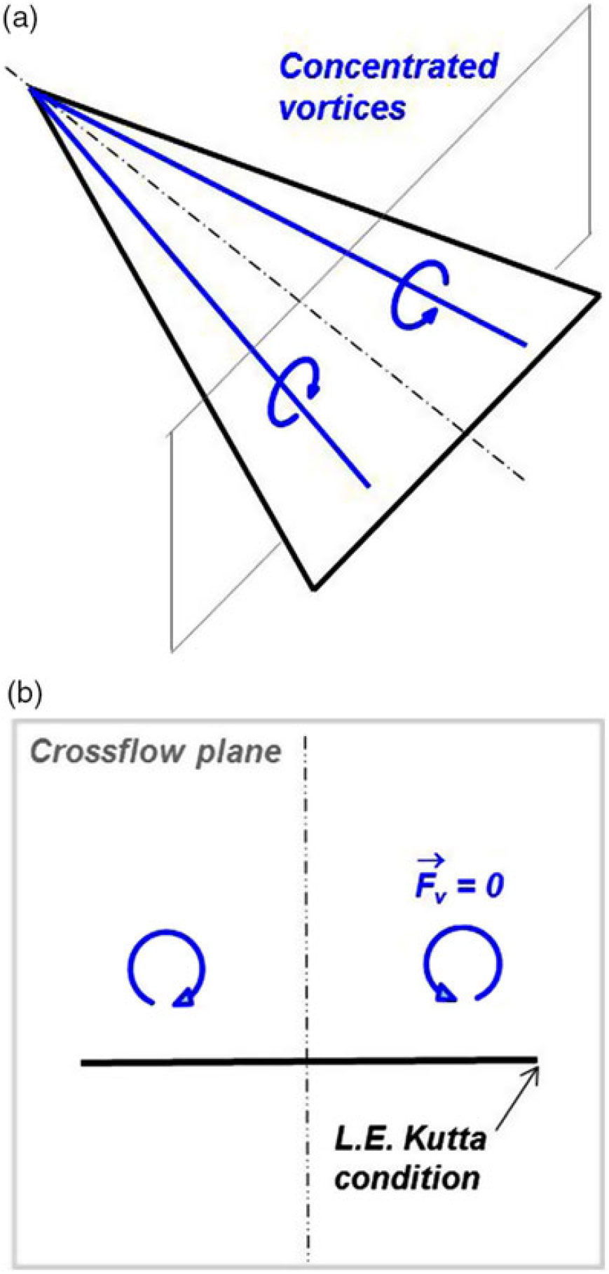
Figure 15. First leading-edge vortex model. Legendre(Reference Legendre31). (a) Concentrated vortices, conical flow. (b) Crossflow plane.
As mentioned in the beginning of Section 5, the sharp leading-edge separation occurs as a spiral vortex sheet that emanates from the highly swept leading edge and rolls up upon itself to form a vortex core over the suction side of the wing. A sketch of this vortex flow, simplified to only the primary vortex, is shown in Fig. 14. The close proximity and coupled nature of this vortex and the wing fundamentally alters the wing flowfield in ways not represented by the Jones attached-flow theory. Theoretical modelling for this primary vortex focused on representing interaction effects between the vortex system and the wing flow. This first led to approximate representations of the vortex sheet with very approximate representations of the vortex core. As the vortex sheet models advanced, more detailed analysis and simulation was performed for the flow within the vortex core itself. The next two subsections address these vortex sheet and vortex core models.
5.1.1 Primary vortex system (conical, 1 vortex)
The first model for a leading-edge vortex interacting with a slender wing was developed by Legendre(Reference Legendre31) in 1952. He formulated the simplest possible representation of the leading-edge vortex i.e., a line vortex with no feeding sheet. With the further assumptions of conical flow about a slender delta wing, he could use a crossflow plane, now including a point vortex, to model the flow with the two-dimensional Laplace equation (Fig. 15). Complex variables were used to solve the flow problem with the usual transformations to satisfy wing boundary conditions. The position and strength of the vortex was determined with the additional boundary conditions that the vortex be force free and that the leading edge satisfies a Kutta condition for smooth off-flow. This last condition provided a compensation for the unmodeled vortex sheet.
Legendre recognised that this model had several deficiencies. Because the leading-edge vortex sheet was not modelled, there was no mechanism for the vorticity to get from the wing into the vortex, and related to this, the vortex strength was not growing longitudinally. His analysis showed some non-physical results at low angles of attack, but also showed positive lift increments due to the vortices that increased nonlinearly with angle-of-attack. In a subsequent publication, Legendre presents some of his thoughts for modelling vortex sheet effects(Reference Legendre32).
Much of the work to follow focused on extending the vortex models to include a representation of the vortex sheet for the conical flow about a slender delta wing. The first extension was due to Brown and Michael(Reference Brown and Michael33) in 1954. Their model included a concentrated line-vortex and a flat feeding sheet of vorticity that connected the line vortex to the sharp leading edge, as seen in Fig. 16. Brown and Michael purposely sought the simplest representation of the leading-edge vortex sheet that could overcome the deficiencies from the Legendre model. Wing vorticity fed the concentrated line vortex, and its strength could grow linearly in the downstream direction. The conical flow was still solved in a crossflow plane using complex variables but with a vortex boundary condition that the net force vanishes for the aggregate vortex system. This was a far-field view towards the force-free leading-edge vortex system that Brown and Michael reasoned was consistent with the locally approximate nature of their vortex model. Despite their simplified model, the vortex boundary condition equations could not be solved analytically and had to be solved in a numerical manner.
The Brown and Michael solutions exhibited suction peaks on the wing’s upper surface that were induced by the vortex system and that moved inboard and became more negative as angle-of-attack increased. The lift from their model was comprised of a linear superposition of the Jones attached-flow solution and a nonlinear vortex-lift increment. Their results also exhibited slender-wing similarity, as shown in Fig. 16. These and other trends from their solution were physically plausible for the slender-wing vortex flow despite the vey approximate representation of their model for the spiral leading-edge vortex system. However, the model overpredicted the vortex-induced effects as compared with experiment.
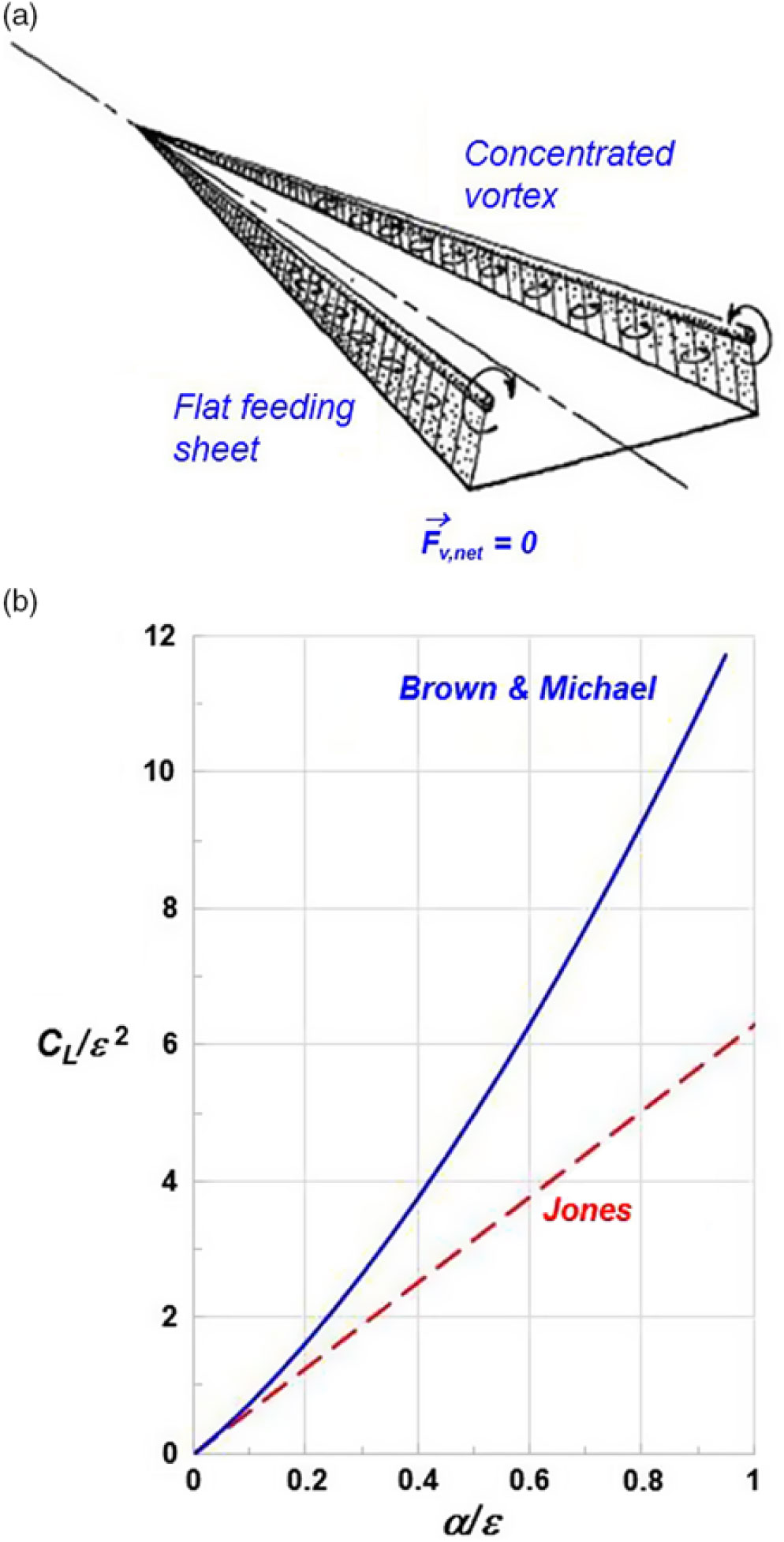
Figure 16. Brown and Michael(Reference Brown and Michael33) model. (a) Flat feeding sheet with concentrated vortex. (b) Lift coefficient predictions.
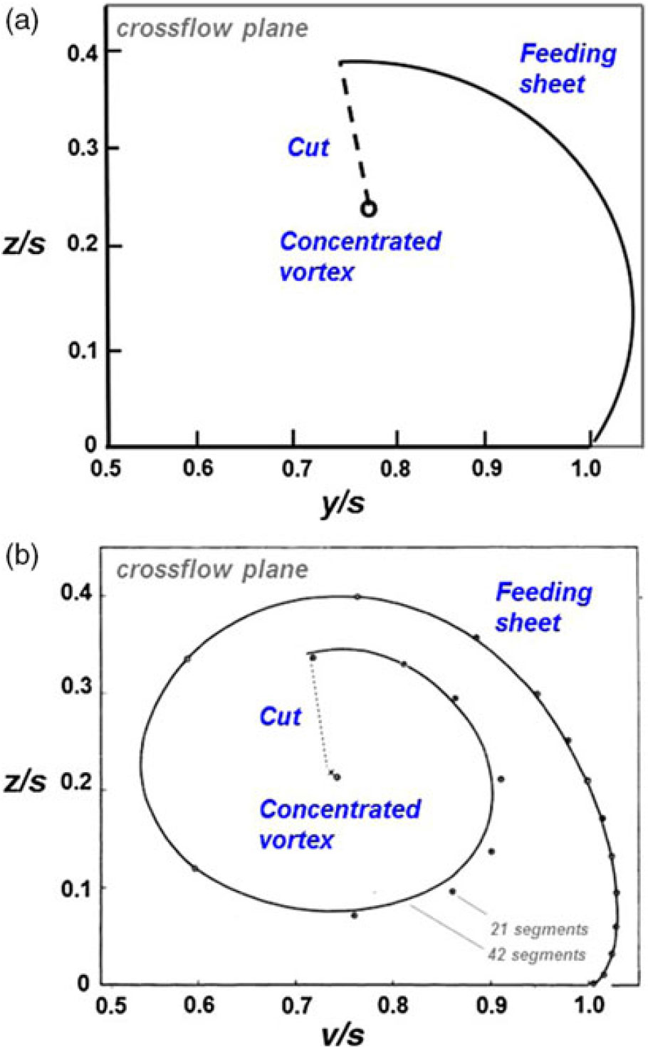
Figure 17. Improved vortex sheet models. (a) Curved feeding sheet, a = 1.2. Mangler and Smith[34]. (b) Segmented feeding sheet, a = 0.91. Smith(Reference Smith35).
In 1959, Mangler and Smith(Reference Mangler and Smith34) further extended the theoretical modelling of the leading-edge vortex system by introducing a curved vortex sheet. Their approach followed the contemporary crossflow plane analysis, but their treatment of the vortex sheet and vortex core in the transformed plane differed from prior work. Mangler and Smith realised that the initial part of the vortex sheet, as observed experimentally, could be approximated in the physical plane by transforming a circular arc from the transformed plane. They further observed that the velocity field due to a simple vorticity distribution on the circular arc could be obtained in the transformed plane. Asymptotic analysis of the inner spiral of the vortex sheet near the centre of the concentrated vortex produced matching criteria between the vortex sheet and the vortex core flows, and the problem closure also included matching criteria between the vortex sheet and the wing at the leading edge. A system of seven simultaneous equations was solved with a combination of analytical and some numerical techniques. An example of the Mangler and Smith vortex sheet solution is shown in Fig. 17(a) for the similarity parameter
 \[{\rm{a}} \equiv \alpha /{\rm{t}}an{\kern 1pt} (\varepsilon ) = 1.2\]
The Mangler and Smith solutions produced less lift than the Brown and Michael results, and above a ≈ 0.5, their leading-edge vortices were further inboard. The corresponding upper surface vortex-induced suction peaks were also further inboard and less negative than the Brown and Michael results, and both trends were in closer agreement to experimental results.
Smith(Reference Smith35) further extended the theoretical modelling of the leading-edge vortex system in 1966 by introducing a segmented vortex sheet. His formulation followed the Mangler and Smith approach, just summarised, but with the notable exception of the vortex sheet representation. Due to the development of the automatic digital computer, Smith could now approximate the vortex sheet with discrete vortex segments. With his method, each segment could now locally satisfy the force-free and streamlined boundary conditions in the process of solving a nonlinear problem for the vortex sheet’s geometry and strength. The vortex core model from Mangler and Smith was retained, and the resultant equations were solved numerically with a sequence of three nested iterations, which addressed the aforementioned vortex sheet conditions as well as the combined vortex cut/vortex core force-free condition. The shape of the vortex sheet no longer required assumptions.
Smith’s model produced a vortex further inboard than the Mangler and Smith model. An example of his solution is shown in Fig. 17(b) for a = 0.91. Vortex-induced suction peaks were further inboard, and less negative, than the Mangler and Smith results. This location of the suction peak also agreed fairly well with experimental results so long as the experimental secondary separation was turbulent, with an example shown later in this paper. The lift from Smith’s solutions was comparable to that of Mangler and Smith, being slightly higher for a < 1.9 (See, Smith(Reference Smith35).)
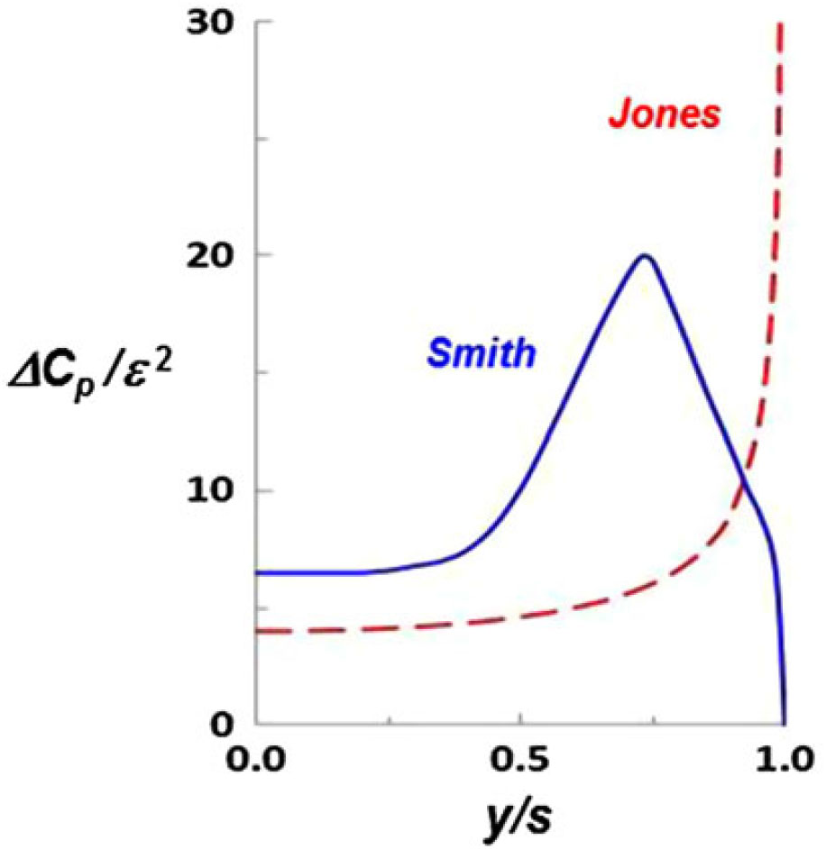
Figure 18. Conical flow pressure distributions for attached (Jones) and leading-edge vortex (Smith) flows. a = 1.
A comparison between the Smith vortex flow solution and the Jones attached-flow solution is shown in Fig. 18. Results are presented in similarity form for a = 1. Twenty years had elapsed from the original Jones slender-wing attached-flow theory to the Smith slender-wing vortex flow theory. From this work, the attached-flow leading-edge singularity had been replaced by a vortex-induced suction peak inboard of the leading edge. The correlation with experimentation improved as the leading-edge vortex system modelling increased in generality, and Smith’s method offered the best correlation of the time. Smith also identified several other vortex flow issues outside the scope of his work, and these included theoretical studies already underway regarding flow in the core of the leading-edge vortex. The vortex sheet models incorporated only a far-field representation of the vortex core, and what was needed was the near-field flow within the core itself that was consistent with the rolling up vortex sheet. The theoretical modelling of this flow will be summarised next.
5.1.2 Primary vortex core
M. G. Hall(Reference Hall30) developed the first model for the flow in the core of a separation-induced leading-edge vortex in 1959, with subsequent refinement and extension(Reference Hall36) in 1961. As with the Mangler and Smith vortex sheet modelling, Hall drew upon experimental work to guide his theoretical vortex core modelling. Flowfield measurements from Harvey(Reference Harvey37) in 1959 had shown that the vortex sheet diffused rapidly as it rolled up above the wing and could not be distinguished after less than one convolution, as much is shown in the Fig. 14 sketch. In addition, the total pressure within the vortex core was approximately axisymmetric with small gradients. Larger total pressure losses were confined to a narrow region near the centre of the vortex.
Hall’s initial model focused on inviscid flow. He reasoned that a continuous rotational flow could approximate some of the vortex core properties being observed in experiments. The rotational inviscid flow is described by the Euler equations, and Hall referred to his model as an Euler vortex. He further assumed an axisymmetric and incompressible flow and a conical velocity field. With these assumptions, the governing partial differential equations, reduced to a coupled system of ordinary differential equations, and an analytical solution was achieved (including a slenderness simplification for convenience). An example solution for Hall’s Euler vortex is shown in Fig. 19. Results are normalised by edge properties, and both the axial and circumferential velocities exhibit forms of logarithmic singularities on the centreline. The high velocities and low pressure within the core qualitatively agreed with experimentally observed trends.
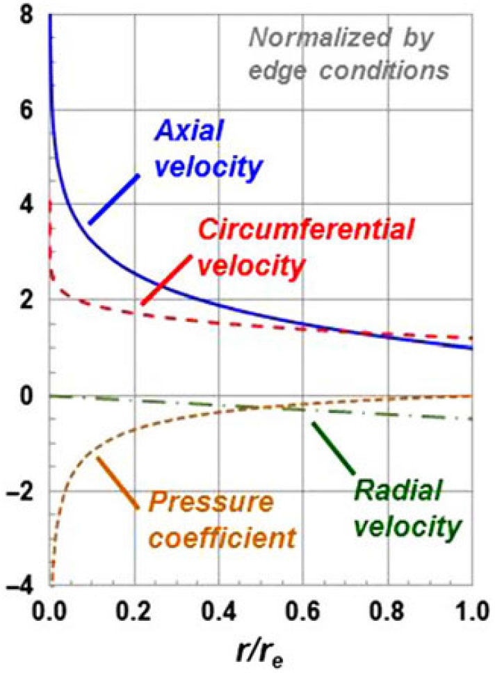
Figure 19. Inviscid incompressible flow in the core of a leading-edge vortex. Axisymmetric, conical flow.
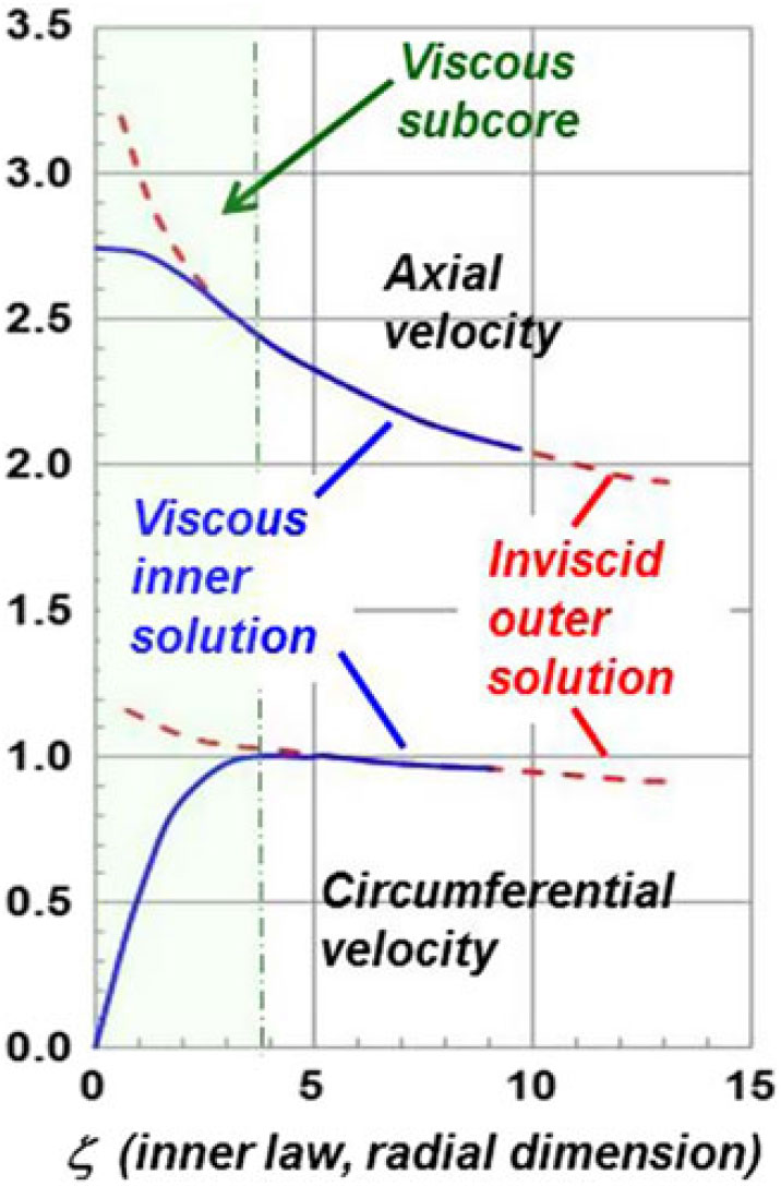
Figure 20. Viscous incompressible flow in the core of a leading-edge vortex. Axisymmetric, conical flow.

Figure 21. Systematic assessments, vortex core flow. (a) Compressible Euler vortex. Brown(Reference Brown39). (b) Nonaxisymmetric analysis. Mangler and Weber(Reference Mangler and Weber40). (c) Compressible, nonaxisymmetric vortex. Brown and Mangler(Reference Brown and Mangler41).
Viscous losses had been shown experimentally to reside in a narrow region near the centre of the vortex, and this implied that boundary-layer analysis could be considered to account for the vortex core viscous flow physics. Hall(Reference Hall36) initiated matched asymptotic analysis to model the viscous flow in 1961, and this work was further advanced by Stewartson and Hall(Reference Stewartson and Hall38) in 1963. The viscous flow effects were assumed to be laminar, so the Euler equations from Hall’s analysis were replaced with the laminar Navier-Stokes equations. All other assumptions from Hall’s prior work were retained; thus, his Euler vortex would serve as the outer solution to the inner viscous vortex solution in the asymptotic sense. Stewartson derived new inner-law variables, and an example of their solution is shown in Fig. 20 for the axial and circumferential velocities as a function of Stewartson’s inner-law variable. An approximate region for the viscous subcore is indicated, based upon the departure of the inner viscous solution from the outer inviscid solution. The viscous subcore is thin and was shown to exhibit an inverse square root dependence on a length Reynolds number. Other dependencies were addressed, and the Stewartson and Hall solution demonstrated that these vortices contain boundary-layer-like scales for the viscous flow physics near the centre of the vortex core. Details of the flow near the centre of the vortex core contribute to vortex breakdown characteristics, and the viscous flow physics there could be important to this phenomenon.
Both the inviscid and viscous vortex core analyses included assumptions of incompressible and axisymmetric flow. Each of these assumptions was subsequently assessed. Brown(Reference Brown39) generalised the Hall Euler vortex to include the effects of compressibility in 1965. All other assumptions from Hall’s Euler vortex analysis were retained. Brown used a combination of analytical and numerical techniques to solve the governing equations. Her solutions showed that compressibility removed the singularity at the axis of the inviscid vortex. An example is shown in Fig. 21(a) for the radial distribution of the circumferential velocity normalised by its edge value. Brown also performed an asymptotic analysis of her solutions for low Mach numbers and showed the presence of a compressibility layer near the axis of the inviscid vortex. Outside this layer, the vortex core flow was effectively incompressible. Brown’s analysis showed that compressibility could be a second source of flow physics affecting vortex breakdown characteristics.
Non-axisymmetric effects were first analysed by Mangler and Weber(Reference Mangler and Weber40) in 1966 for the incompressible Euler vortex. All other assumptions from Hall’s Euler vortex analysis were retained. Mangler and Weber contrasted the continuous rotational flow from Hall’s Euler vortex with the flow generated by a spiral vortex sheet imbedded in a potential flow, shown in Fig. 21(b). Asymptotic expansions for the non-axisymmetric effects were formulated for the spiral vortex sheet, and Mangler and Weber showed that the leading axisymmetric term in their solution was identical to Hall’s axisymmetric solution. The non-axisymmetric effects were manifested in the higher order terms of their expansion.
Brown and Mangler(Reference Brown and Mangler41) further assessed non-axisymmetric effects for the compressible Euler vortex in 1967. Compressibility was added to the spiral vortex sheet modelling from Mangler and Weber, and the flow was solved with asymptotic methods. The compressible vortex sheet was shown to be less tightly wound as compared to the incompressible case. Comparisons were also made with Brown’s compressible Euler vortex, and one example is shown in Fig. 21(c). The chart shows the radial distribution of the normalised circumferential velocity, and the jumps in the spiral vortex sheet solution were cantered about the continuous rotational solution. The models produced consistent solutions in the outer region of the vortex core. Near the centreline, the swirl velocity from the inviscid Euler vortex decreased to zero due to the aforementioned compressibility effects.
All these vortex core studies had retained the conical flow assumption to facilitate analytically-based radial assessments of various flow physics effects. Amongst these, viscosity was shown to introduce a boundary-layer type of structure within the vortex core. Following boundary-layer solution techniques, Hall(Reference Hall42) formulated a numerical method in 1967 to compute the longitudinal progression of high Reynolds number swirling flows. The flow was assumed to be incompressible and axisymmetric, and Hall removed the conical flow assumption in favour of a longitudinal marching technique similar to other boundary-layer solution methods. The work focused on laminar flow, and by virtue of boundary-layer approximations, the governing Navier-Stokes equations reduced to a system of parabolic equations. Hall referred to the resulting flow as quasi-cylindrical. The method required radial distribution of initial conditions, and the flow could be marched downstream subject to edge boundary conditions. His approach allowed for variations in the edge geometry, which could be either stipulated or solved for.

Figure 22. Quasi-cylindrical vortex core solution examples. Hall(Reference Hall42). (a) Trailing-vortex application. (b) Leading-edge vortex application.
Two of Hall’s test cases are shown in Fig. 22. The first case was for a trailing vortex, such as forms in the wake of a lifting wing. Initial conditions were taken from an approximate theory due to Newman(Reference Newman43), and boundary conditions were held constant. The solution shows the viscous decay of the axial velocity deficit as well as the swirl velocity plotted as a function of the similarity-scaled radial coordinate,
 \[{\rm{R}} = {\rm{R}}{e^{(1/2)}}{\kern 1pt} {\rm{r}}.\]
The correlation between the Hall results and the Newman theory were as expected, with the difference in axial decay being due to additional effects included in the Hall formulation.
The second test case from Hall’s work is for a slender-wing leading-edge vortex. Initial conditions were obtained from the Stewartson and Hall(Reference Stewartson and Hall38) theory. Boundary conditions included a conical bounding geometry with constant flow properties (50 < × <100) followed by an adverse pressure gradient region where the bounding stream tube became part of the solution (100 < × < 140). The boundary conditions were chosen to mimic conditions that could be realised on a three-dimensional delta wing, and the velocity profiles within the vortex core exhibited consistent trends. An example of coupling Hall’s quasi-cylindrical vortex core with a three-dimensional leading-edge vortex simulation will be shown later in this paper.
Many aspects of the leading-edge vortex flow were learned through the conical and quasi-cylindrical studies of the detailed flow within the vortex core and the conical studies of the aggregate flow from the vortex sheet/approximate vortex core models. However, there remained a need for solutions that were three dimensional and that could be applicable to wing aerodynamics. The next section summarises a number of these methods.
5.2 Three-dimensional flows, sharp edge, 1 vortex
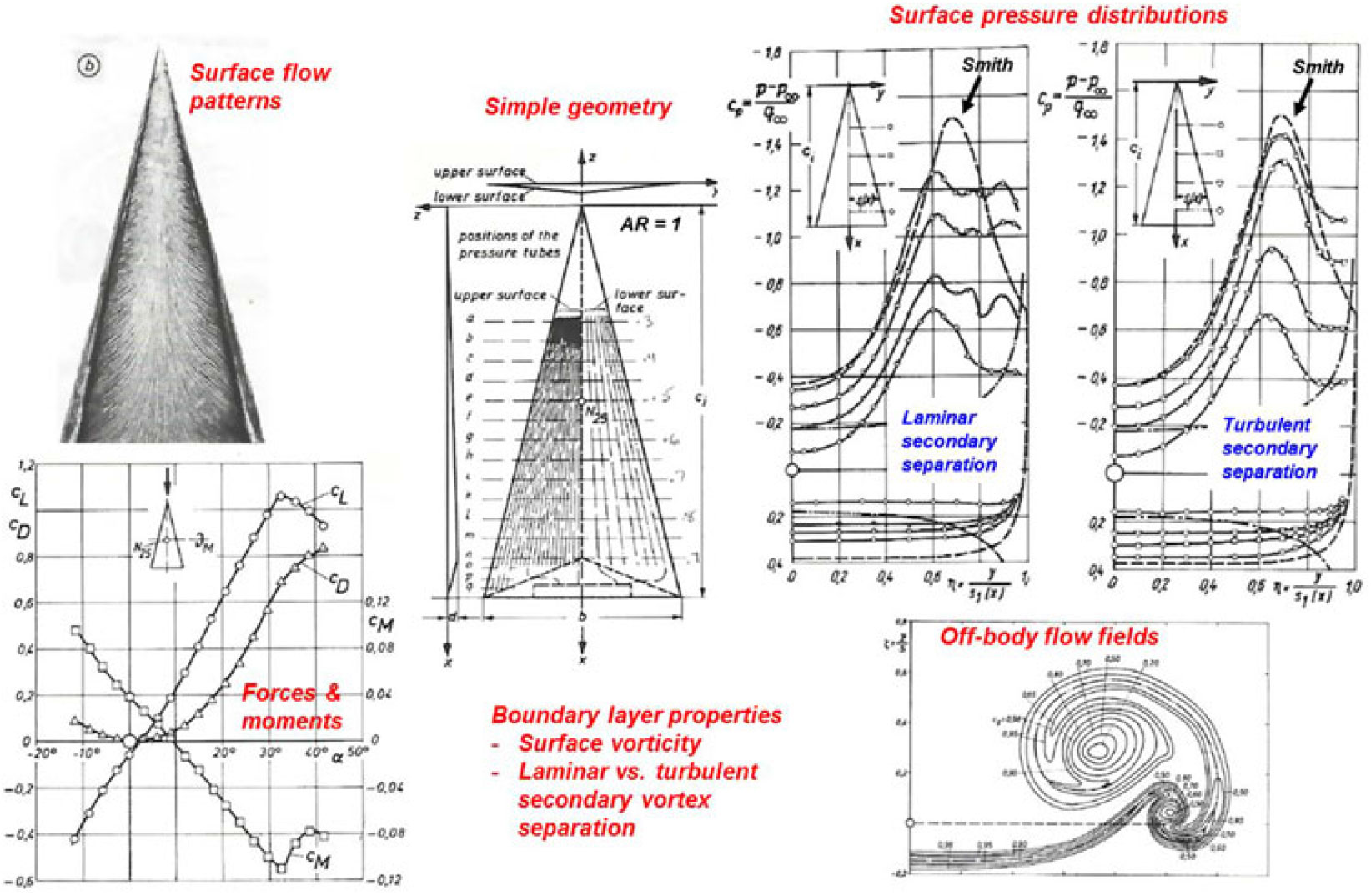
Figure 23. Experimental guidance, Hummel(Reference Hummel25) delta wing. AR = 1.0, M ≈ 0.
Very detailed experiments on a unit aspect ratio delta wing were performed by Hummel with initial reporting(Reference Hummel44) in 1965 and summary reporting(Reference Hummel25) in 1979. This work documented many details of the flow physics associated with the leading-edge vortex flow from a three-dimensional delta wing. A summary of some of Hummel’s results is shown in Fig. 23. Amongst these results are spanwise surface pressure distributions at different percent chord locations from the apex to the trailing edge (upper-right of Fig. 23). The Smith(Reference Smith35) conical flow solution for this wing is also shown, and the nonconical three-dimensional effects, mostly due to the trailing edge, are significant. Hummel’s results also demonstrate the effect of the boundary-layer state (laminar or turbulent) on secondary vortex separation. The turbulent secondary vortex is much smaller than the laminar one and has less effect on the primary vortex. The inviscid Smith theory provides a reasonable estimate of the primary vortex suction peak from Hummel’s turbulent experimental results at the forwards most station shown, but it is clear that the conical flow theory does not represent the three-dimensional wing loads.
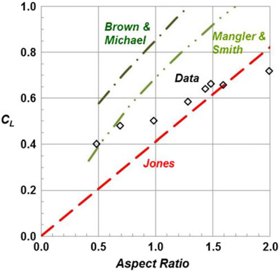
Figure 24. Aspect ratio effect on delta wing lift coefficient. M ≈ 0, α = 15°.
A second example for three-dimensional effects of sharp-edged delta wings with leading-edge vortices is shown in Fig. 24. In this figure, the lift coefficient is shown as a function of the aspect ratio for a fixed angle-of-attack that would include vortex-lift effects. Several of the conical flow theories are included, and the data are from various sources(Reference Polhamus45). The conical vortex flow theories overpredict the data for most of the conditions shown and do not capture the trend with aspect ratio. (The Jones attached-flow theory is shown only for reference).
The conical flow research was critical to advancing the understanding of the structure of separation-induced leading-edge vortices. In a sense, this could be a slender-wing analogue to the utility of aerofoil research in understanding high-aspect-ratio wing aerodynamics. Experimental guidance had demonstrated the need for three-dimensional methods that would account for the leading-edge vortex effects on wing aerodynamics, and these methods are reviewed next.
5.2.1 Modelling for vortex effects
Two modelling approaches are summarised. The first provided force and moment estimates through an analogy to wing edge forces. The second provided three-dimensional pressure predictions from a model of the free-vortex-sheet.
5.2.1.1 Leading-edge suction analogy
In 1966, Polhamus(Reference Polhamus45) proposed a method to compute delta wing forces and moments that accounted for the leading-edge vortex contributions through a leading-edge suction analogy. There were two key aspects to his approach. The first was a connection between the leading-edge suction force developed in attached flows and the leading-edge vortex force developed in the separation-induced vortex flows. Polhamus’s reasoning came in part from attached-flow conservation of leading-edge suction principles. He considered the condition for which the vortex first formed very near the leading edge and induced flow reattachment, Fig. 25. The bulk of the wing streamlines remained unaltered, and in this case, Polhamus conjectured that the suction force that was present in attached flow would be sustained but reoriented for the vortex flow to act normal to the wing surface at the leading edge. By this suction analogy, the vortex-induced normal forces were related to the attached-flow edge forces, and these edge forces could be computed with attached-flow methods of that time, such as a vortex lattice. The second aspect of his method was to fully account for high angle-of-attack effects in force vector orientations.

Figure 25. Concept for Polhamus leading-edge suction analogy. Polhamus(Reference Polhamus45).
The theory was incorporated into several vortex lattice methods(Reference Margason and Lamar46, Reference Lamar and Gloss47) formulated for the high angle-of-attack boundary conditions and for edge-force analysis suitable to extract the necessary constants in the Polhamus theory. The vortex lattice method accounted for three-dimensional planform effects along with twist and camber effects and solved the linear Prandtl-Glauert equation to account for linear compressibility. With his approach, only a single solve was necessary to extract the constants for attached-flow and separated-flow forces and moments, and the high angle-of-attack formulation then provided the force and moment trends with angle-of-attack. For example, by the Polhamus formulation, the lift from the attached flow and vortex flow took on the form
 \[\begin{array}{c}{{\rm{C}}_{{\rm{L}},p}} = {{\rm{K}}_{\rm{p}}}{\kern 1pt} {\rm{c}}o{s^2}(\alpha ){\kern 1pt} {\rm{s}}in(\alpha ) \\ {{\rm{C}}_{{\rm{L}},v}} = {{\rm{K}}_{\rm{v}}}{\kern 1pt} {\rm{s}}i{n^2}(\alpha ){\kern 1pt} {\rm{c}}os(\alpha ) \end{array}\]
and these were superimposed for the total lift
 \[{{\rm{C}}_{\rm{L}}} = {{\rm{C}}_{{\rm{L}},p}} + {{\rm{C}}_{{\rm{L}},v}} = {{\rm{K}}_{\rm{p}}}{\rm{c}}o{s^2}(\alpha ){\kern 1pt} {\rm{s}}in(\alpha ) + {{\rm{K}}_{\rm{v}}}{\kern 1pt} {\rm{s}}i{n^2}(\alpha ){\kern 1pt} {\rm{c}}os(\alpha )\]
In these equations, K p and K v are the configuration specific constants extracted from the vortex lattice solution. Since the leading-edge thrust is no longer manifested in the plane of the wing, the drag was given by
 \[{{\rm{C}}_{\rm{D}}} = {{\rm{C}}_{\rm{L}}}{\kern 1pt} {\rm{t}}an(\alpha )\]
Although, in this drag relationship, the lift coefficient and angle-of-attack include the vortex-lift effects. A status of the initial suction analogy formulation and assessments was given by Polhamus(Reference Polhamus48) in 1971.
A first example for the Polhamus suction analogy predictions is shown in Fig. 26. In this figure, the conical vortex flow theories and data are repeated from Fig. 24, and the high-α linear theory and suction analogy results from the Polhamus formulation are added. The correlation between the data and Polhamus’s suction analogy is very good.
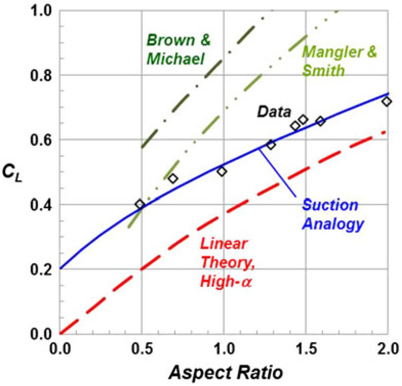
Figure 26. Aspect ratio effect on delta wing lift coefficient. M ≈ 0, α = 15°. Polhamus(Reference Polhamus45).
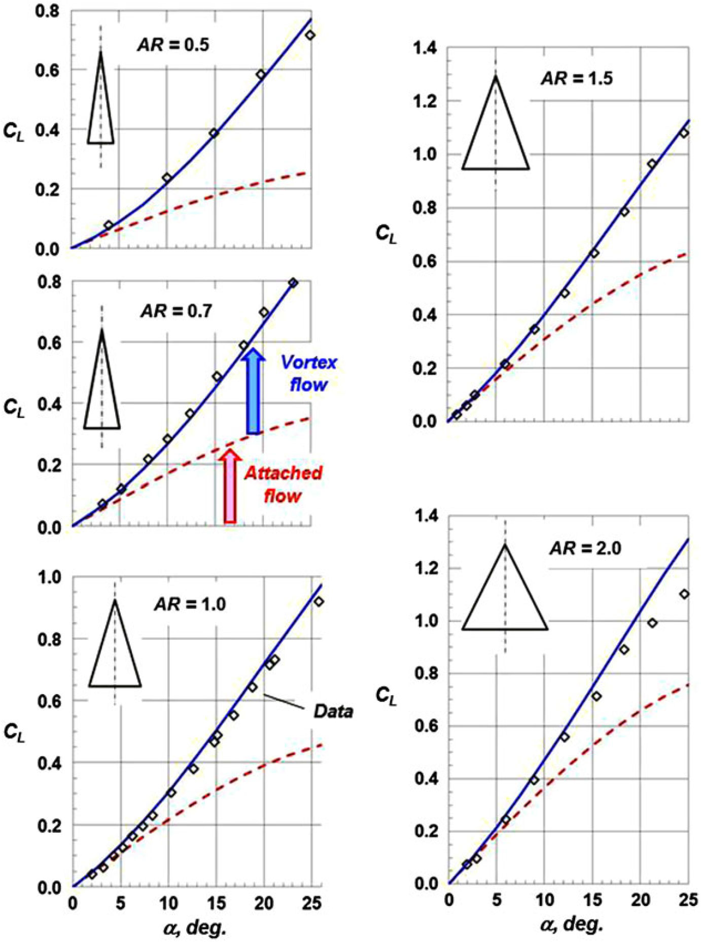
Figure 27. Vortex-lift predictions, delta wings. M ≈ 0. Polhamus(Reference Polhamus45).

Figure 28. Effect of Mach number, delta wing lift and drag coefficients, AR = 1. Polhamus(Reference Polhamus49).
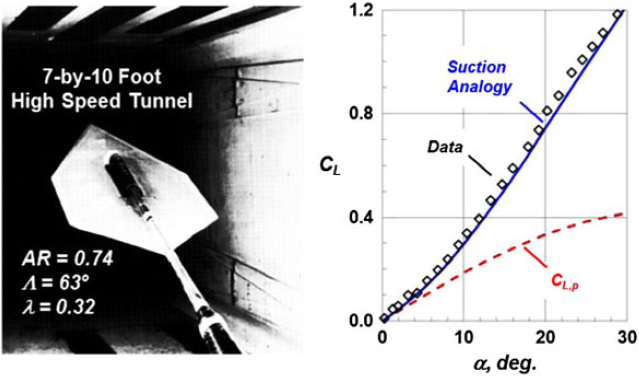
Figure 29. Extension for complex planform effects. Lamar(Reference Lamar50, Reference Lamar51).
Comparisons between the suction analogy and experiment for the lift coefficient variation with angle-of-attack are shown in Fig. 27 for a range of delta wing aspect ratios. The correlation was surprisingly accurate, and in the case of the AR = 2 delta wing, the departure between experiment and the suction analogy was likely due in part to vortex breakdown effects. The Polhamus suction analogy produced the first accurate and general vortex-lift predictions for delta wings.
Application of the Polhamus theory was not limited to low speeds, and an example of supersonic assessments is shown in Fig. 28. The AR = 1 delta wing would have a sonic leading edge at M = 4.12, and for the supersonic cases shown, the leading edge would still be subsonic. The correlation with experiment for the total lift coefficient was good, and the results demonstrated the reduction in vortex-lift increments associated with Mach cone proximity to the leading edge. The induced drag parameter was also well predicted over the lift coefficient range. The induced drag for the vortex flow condition is always higher than the attached-flow (full thrust) case, and yet the vortex lift reduces this penalty.
Extensions for more complex wing analysis were also developed. In 1974, Lamar extended the Polhamus theory to include separation-induced side-edge vortices(Reference Lamar50) and again in 1975 for additional planform effects(Reference Lamar51). An example from his work for a cropped diamond wing is shown in Fig. 29, and the correlation with lift coefficient was again quite good. Experimentation was an integral part of the theoretical suction analogy work, and the data in Fig. 29 came from a test program conceived and executed by Lamar in the National Aeronautics and Space Administration (NASA) Langley 7-by-10ft high-speed tunnel(Reference Fox and Huffman52).
The method was also extended for more complex configuration analysis, and an example from Luckring(Reference Luckring53) for a strake-wing application is shown in Fig. 30. For this configuration, two leading-edge vortices were generated, one from the strake and the other from the wing, and the component loads were isolated between the forebody-strake and aftbody-wing portions of the configuration. A number of strake sizes and wing sweeps were included in the program. The suction analogy was modified to model the weak vortex-interaction condition (low angles of attack) and approximate the strong vortex-interaction condition (high angles of attack), and correlations with experiment in general were good. The rapid break in the data from the suction analogy estimates was due to near-field vortex breakdown effects. Here again, an experimental program was conducted by Luckring to guide his theoretical suction analogy research. Motivation for the strake-wing research came from the light-weight fighter interests in the US, which had led to the General Dynamics YF-16/F-16 and the Northrop YF-17 aircraft. These aircraft had recently been developed, and the research contributed understanding of the strake-wing vortex flows.
Other configuration assessments with the Polhamus suction analogy were generally useful in estimating forces and moments. Force estimates, such as shown herein, were fairly common, and moment estimates were not always as accurate but were still useful, and the computations were simple to set up and quick to process on contemporary computers. However, a need remained to predict surface pressure distributions for wings with separation-induced leading-edge vortex flows, and this led to the development of a free-vortex-sheet method discussed next.

Figure 30. Extension for component loads. Luckring(Reference Luckring53).
5.2.1.2 Vortex sheet modelling
A three-dimensional free-vortex-sheet model was developed by Brune et al.(Reference Brune, Weber, Johnson, Lu and Rubbert54) in 1975, and the basic concept for this model is illustrated in Fig. 31. The formulation is based on a panel method used to solve the Prandtl-Glauert equation, and it includes both a panel representation of the wing as well as a panel representation of the leading-edge vortex. The leading-edge vortex model was essentially a three-dimensional implementation of Smith’s(Reference Smith35) conical flow model. The leading-edge vortex was comprised of a force-free vortex sheet that was terminated by a cut that fed vorticity to a line vortex at its free edge. Higher-order singularity distributions of either quadratic doublet distributions or linear source distributions were used to create distributed-load panels to model the flow. The vortex geometry and strength had to be solved along with the wing loads, and this nonlinear problem was solved with a modified Newton method to obtain iterative convergence. More complete documentation of this approach was given by Johnson et al.(Reference Johnson, Lu, Tinoco and Epton56) in 1980.
A sample result from this free-vortex-sheet formulation is shown in Fig. 32 from Gloss and Johnson(Reference Gloss and Johnson55). Results in this figure include conical flow predictions for attached-flow (Jones[12]) and leading-edge vortex flow (Smith(Reference Smith35)), measurements from Marsden(Reference Marsden, Simpson and Rainbird57) and the free-vortex-sheet predictions. Correlation between the free-vortex-sheet results and the experimental results are generally good and clearly show the three-dimensional effects as contrasted with the conical flow result from Smith. Differences between the (inviscid) free-vortex-sheet predictions and experiment were primarily associated with secondary vortices, a viscous flow phenomenon. Similar free-vortex-sheet models were developed at the Netherlands Aerospace Center (NLR) by Hoeijmakers(Reference Hoeijmakers and Bennekers58, Reference Hoeijmakers59) and at Dornier by Hitzel(Reference Hitzel and Wagner60).

Figure 31. Free-Vortex-Sheet model, FVS.

Figure 32. Free-vortex-sheet prediction of delta wing pressure coefficients. AR = 1.46, M ≈ 0, α = 14°. Gloss and Johnson(Reference Gloss and Johnson55).

Figure 33. Pressure, force and moment predictions from free vortex sheet. Hummel delta wing, AR = 1.0, M ≈ 0. Luckring(Reference Luckring61).
A second example of free-vortex-sheet predictions is taken from a survey paper by Luckring(Reference Luckring61) that included application to the Hummel delta wing, as seen in Fig. 33. In addition to surface pressure correlations, this result showed force and moment correlations, and the correlations were generally very good. Discrepancies in the pressure distributions were attributed to unmodeled secondary vortex effects. The rapid break in the force and moment data at a high angle-of-attack was attributed to vortex breakdown.
From these assessments as well as others, it became clear that representation of the separation-induced leading-edge vortex by the free vortex sheet with the approximate vortex core model was sufficient to model the three-dimensional inviscid wing pressures as well as forces and moments, at least for simple wing planforms, so long as vortex breakdown was absent from the wing nearfield. The occurrence of vortex breakdown in the nearfield of the wing generally resulted in significant, and often undesirable, changes in force and moment properties. One example is shown in Fig. 33. The vortex breakdown flow physics included details of the viscous and rotational flow within the vortex core, and these vortex core flow details were absent from the three-dimensional theoretical methods discussed. Two critical issues to predict for the high angle-of-attack wing aerodynamics were (i) the angle-of-attack where vortex breakdown advanced from downstream to the wing trailing edge and (ii) the subsequent wing aerodynamics at higher angles of attack. One approach to predict the onset of vortex breakdown to the wing nearfield is presented in the next section.
5.2.1.3 Coupled vortex sheet/vortex core modelling
Luckring(Reference Luckring62) extended the separation-induced leading-edge-vortex modelling in 1985 by coupling the free-vortex-sheet method(Reference Johnson, Lu, Tinoco and Epton56) with Hall’s(Reference Hall42) quasi-cylindrical vortex core model. The Stewartson and Hall(Reference Stewartson and Hall38) conical formulation was used to provide initial conditions in a manner suitable to the three-dimensional free-vortex-sheet simulation. Also, asymptotic analysis following the Mangler and Weber(Reference Mangler and Weber40) work established a boundary condition approach to couple the axisymmetric viscous and rotational vortex core with the three-dimensional inviscid free-vortex-sheet simulation. Overall, this was analogous to matching an inner boundary layer formulation with an outer inviscid formulation. This approach put the vortex core flow physics from Hall into a three-dimensional environment.

Figure 34. Pressure, force and moment predictions from free vortex sheet. Hummel delta wing, AR = 1.0, M ≈ 0. Luckring(Reference Luckring61).
An example from Luckring’s(Reference Luckring62) coupled formulation is shown in Fig. 34. Correlation with flowfield measurements from Earnshaw(Reference Earnshaw63) are shown in the lower left portion of the figure and were considered to be reasonable. Luckring assessed a number of vortex breakdown criteria, and an example of predictions for the angle-of-attack for vortex breakdown to cross the wing trailing edge is shown in the lower right portion of the figure. The Ludweig(Reference Ludweig64) critical helix angle was used as a burst criterion, and the vortex breakdown data are due to Wentz(Reference Wentz and Kohlman65). The data show a strong sensitivity to delta wing leading-edge sweep variations and a weak sensitivity to trailing-edge sweep variations. The results from Luckring’s coupled analysis approximated both trends. Although this seemed to provide a predictive criterion for the onset of near-field vortex breakdown, computations for the details of the burst vortex were beyond the scope of the model.
The free-vortex-sheet formulation was generally successful in predicting the three-dimensional pressures as well as forces and moments on configurations with separation-induced leading-edge vortices. The computations were, however, cumbersome. Convergence could be difficult for some applications, and the applications were, in general, restricted to relatively simple wing shapes. During the time of this three-dimensional vortex modelling research, a new capability was emerging that offered promise to capture vortical flows. This became a paradigm shift for computational vortex flow aerodynamics and is the topic of the next section.
5.2.2 Models that capture vortex effects
In 1981, Jameson, Schmidt and Turkel(Reference Jameson, Schmidt and Turkel66) developed a finite-volume approach to numerically solve the three-dimensional Euler equations with a multistage Runge-Kutta integration scheme. This technique provided a new and general capability for computing rotational as well as irrotational flows. Prior to this accomplishment, three-dimensional CFD methods had been developed for solving complex but irrotational flows (e.g., flows modelled with the full potential or transonic small disturbance equations), and these methods could be applied to relatively complex geometries. Rotational effects had required explicit treatment, such as with the vortex sheet modelling just discussed. With the new Euler equation solution technique, vortices could, in principle, be captured implicitly as opposed to being modelled explicitly. Many solvers were developed exploring variations on the Jameson/Schmidt/Turkel inviscid approach, and the solver technology also led rather quickly to methods for solving viscous flows with the three-dimensional Navier-Stokes equations.
The change from explicit vortex modelling to implicit vortex capturing constituted a paradigm shift for computing separation-induced leading-edge vortex flows. The new capability also came with new questions. A summary for the leading-edge vortex analysis with these new methods is provided below. The results include not only the Euler and Navier-Stokes analysis, but also the emergent analysis with hybrid Reynolds-Averaged Navier Stokes (RANS)/ Large Eddy Simulation (LES) methods.
5.2.2.1 Euler analysis
Analysis in this section consists of the numerical solution of steady, inviscid rotational flows. The solution techniques for the Euler equations required the addition of artificial dissipation terms (also known as artificial viscosity) for stabilisation. A blend of second- and fourth-order damping terms was customary, and the damping would manifest in high-gradient regions, such as at the leading edge of an aerofoil. The Euler equations admit non-isentropic flows, so the numerical Euler solutions could include not only physics-based entropy production, such as from a shock wave, but also numerically-based entropy production from the artificial viscosity. Entropy generation will correspond to total pressure losses. The spurious numerical entropy was a new concern both for numerical error assessments and for aerodynamic simulation effects. Many fundamental analyses were performed, with one example given by Rizzi(Reference Rizzi67) in 1984 for spurious entropy generated near the leading edge of aerofoils.

Figure 35. Grid resolution effect, blunt-leading-edge delta wing. Λ = 70°, 14:1 elliptic cross section, M = 2, α = 10°, βcotΛ = 0.630. Newsome(Reference Newsome68).
Spurious entropy can have significant consequences for leading-edge vortex simulations from wings with a finite leading-edge radius, an example of which was shown by Newsome(Reference Newsome68) in 1985, as seen in Fig. 35. Newsome modelled the conical Euler equations for supersonic flow so that only the crossflow plane needed discretisation. Computations were performed with a research code, and his studies included grid refinement effects for grids that ranged between 0.004 m and 0.010 m cells. Solutions were obtained for a 14:1 elliptical cone with a subsonic leading edge. This created a leading-edge radius representative of thin aerofoils. Newsome’s coarse grid results demonstrated that the numerical damping introduced a spurious vortex in association with a numerically-induced separation at the wing’s leading edge. Finer grids required less numerical damping, and with enough grid resolution the flow around the leading edge remained attached and the solution produced a crossflow shock, now with physics-based entropy from the shock.
Spurious entropy had smaller effects on leading-edge vortex simulations from wings with sharp leading edges. Powell(Reference Powel69) also modelled the conical Euler equations for supersonic flow and completed detailed numerical assessments for sharp-edged delta wings in 1987. Powel showed that the overall vortex structure was nearly independent of numerical parameters and was sustained in grid convergence studies. Total pressure losses occurred in the vicinity of the vortex sheet and core, and the magnitude of total pressure loss was also insensitive to numerical parameters. Numerical effects were restricted to fine-scale structures within the vortex without significantly altering the macro-scale vortex properties.
Hoeijmakers and Rizzi(Reference Hoeijmakers and Rizzi70) compared free-vortex-sheet modelling and Euler simulations for a sharp-edged delta wing in 1984. The authors chose a 70° flat-plate delta wing at 20° angle-of-attack and incompressible flow for their study. These conditions would avoid vortex breakdown and have small secondary vortex effects. The free-vortex-sheet simulation used 468 panels in total, while the Euler simulation used 0.08 m cells to represent the flow. Correlations for the vortex geometry between the two formulations were very good and the correlations for the wing surface pressures were plausible. The total pressure loss within Euler-simulated vortex did not seem to significantly alter wing surface pressures. One example is shown in Fig. 36.
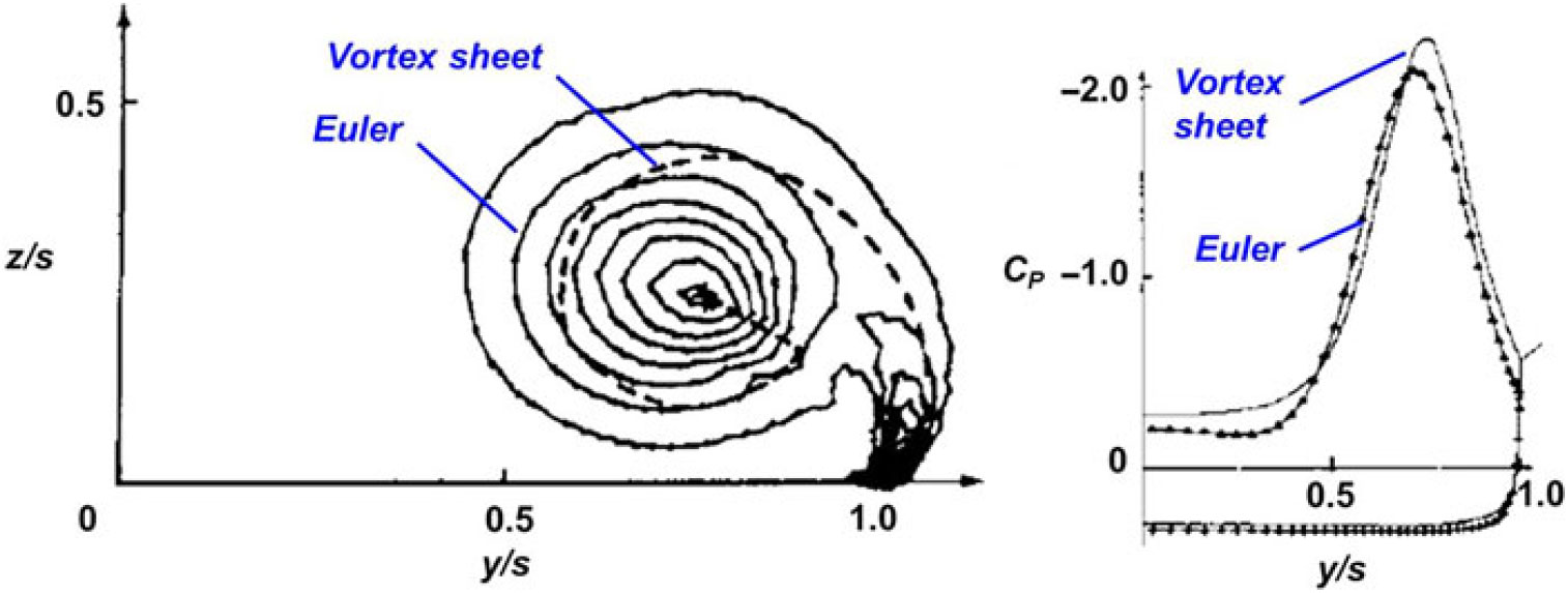
Figure 36. Euler and vortex sheet predictions. 70° delta wing, x/c r = 0.6, M = 0, α = 20°. Hoeijmakers and Rizzi(Reference Hoeijmakers and Rizzi70). (Copyright 1984 by AIAA. Adapted with permission.)
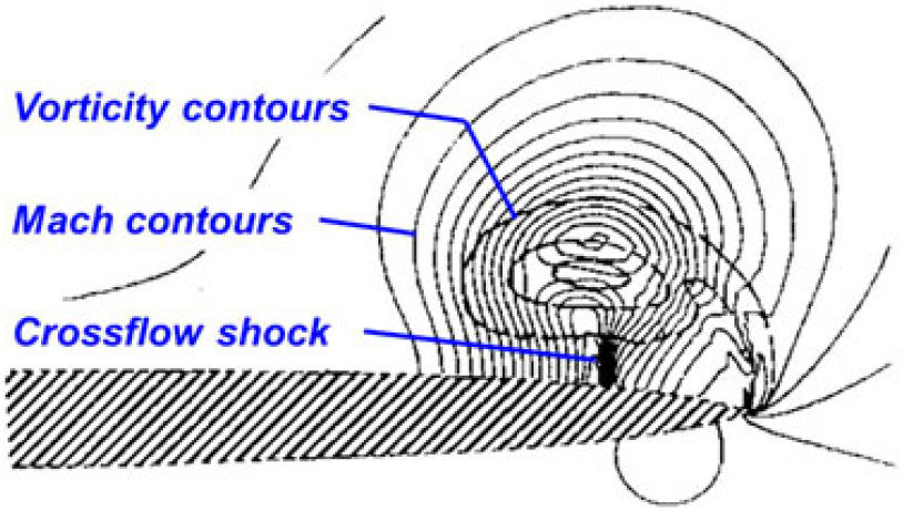
Figure 37. Euler prediction, Dillner delta wing. Λ = 70°, x/c r = 0.80, M = 0.7, α = 15°, fine grid. Rizzi(Reference Rizzi71). (Copyright 1984 by A. Rizzi. Adapted with permission.)
The Euler equations can capture both shocks and vortices, and Rizzi(Reference Rizzi71) demonstrated transonic shock-vortex interactions in 1984 for a 70° nonconical delta wing that had a 6% thick biconvex aerofoil section with sharp edges (also known as the Dillner wing). Computations were presented for M = 0.70 and M = 1.50 at a = 15° with a then-standard but relatively coarse grid of 0.04 m points and a fine grid of 1.07 m points. The fine grid was important to resolving flow details, and one example is shown in Fig. 37 for the M = 0.7 case. The results show vorticity and Mach contours superimposed at the 80% chord station, and with the fine grid solution a crossflow shock was resolved between the vortex and the wing. In the coarse-grid solution, the crossflow shock was not present, and the vortex was more diffused although the vortex core location was about the same.
It is also worth noting that during 1984 to 1986 a campaign was executed to provide new experimental data for Euler code assessments with a cropped-delta-wing configuration. The campaign was known as the International Vortex Flow Experiment, or Vortex Flow Experiment 1 (VFE-1), and summary reports for this effort were given in 1988 by Drougge(Reference Drougge72) for the program, by Elsenaar et al.(Reference Elsenaar, Hjelmberg, Büttefisch and Bannink73) for experiments and by Wagner et al.(Reference Wagner, Hitzel, Schmatz, Schwarz, Hilgenstock and Scherr74) for computations. Further analysis has been reported by Elsenaar and Hoeijmakers(Reference Elsenaar and Hoeijmakers75) in 1991.
In the early 1980s, computational abilities were rapidly expanding to include three-dimensional solutions of the Navier-Stokes equations, and highlights from that work are presented next.
5.2.2.2 Navier stokes analysis
The Euler solution technology established a path to solving the three-dimensional RANS equations. The principle challenges were the high computational cost associated with resolving small-scale viscous effects as well as the need to model turbulence in an approximate manner. Solution techniques focused on the thin-layer approximation to the RANS equations as one means to reduce viscous resolution needs and improved grid generation technology provided a second means. Improved algorithms were also developed while supercomputers sustained growth in both speed and capacity. Collectively, these trends made the numerical solution of the three-dimensional thin-layer Navier-Stokes equations feasible in a very few years following the breakthrough Euler solution technology. Analysis for this section will focus on the numerical solution of steady viscous rotational flows.
Early contributions came from Fujii and Kutler(Reference Fujii and Kutler76, Reference Fujii and Kutler77) in 1983 (using an older Beam and Warming approach(Reference Beam and Warming78)) and 1984 (using an older Pulliam and Steger approach(Reference Pulliam and Steger79)) for numerically solving the thin-layer Navier-Stokes equations for leading-edge vortex flows about several geometries at subsonic speeds. Depending upon the application, the chord Reynolds number was on the order of 1m to 6m, and the three-dimensional grids had approximately 0.030 m or 0.060 m points. The field grid resolution was coarse, but the solutions converged and included three-dimensional viscous effects for the vortex flows.
In 1985, Thomas et al.(Reference Thomas, van Leer and Walters80, Reference Thomas and Walters81) developed an upwind flux-split algorithm for solving Euler and thin-layer Navier-Stokes equations, and this formed the basis for the upwind-biased finite volume code CFL3D(Reference Biedron and Thomas82). In 1986, Thomas and Newsome(Reference Thomas and Newsome83) exploited the conical flow equations to study supersonic viscous vortex flows. Because of the conical flow assumption, high grid resolution was achieved in the crossflow plane with only 0.011 m points. Results were presented as Reynolds numbers on the order of one million for supersonic vortical flows about several geometries. Accurate correlations with the experiment were achieved, and one example is shown in Fig. 38 using new experimental results published by Miller and Wood(Reference Miller and Wood84) in 1983.
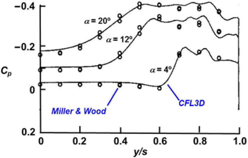
Figure 38. Supersonic vortex flow, CFL3D. Λ = 75° delta wing, M = 1.7, Re cr = 3.6×10⁶. Thomas and Newsome(Reference Thomas and Newsome83).
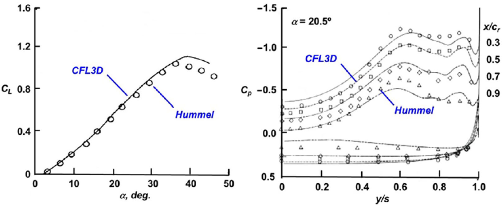
Figure 39. Laminar Navier-Stokes predictions, CFL3D. AR = 1 Hummel delta wing, M = 0.3, Re cr = 0.95×10⁶. Thomas et al.(Reference Thomas, Taylor and Anderson85).
Subsonic assessments were subsequently performed by Thomas et al.(Reference Thomas, Taylor and Anderson85) for viscous vortex flows in 1987 using the Hummel delta wing. A dominant viscous flow phenomenon is the secondary vortex, which has large effects on the combined primary-secondary vortex system when the secondary vortex separation is laminar. Thomas chose to compute this case with a baseline grid of 0.55 m points and included grid resolution assessments. Comparisons with the experiment are shown in Fig. 39, and the viscous flow simulation predicted CL,max fairly close to experiment. The predicted surface pressures also correlated fairly well with Hummel’s measurements. With Thomas’s work, the capability to compute viscous vortex flows at subsonic and supersonic speeds with good accuracy had been established for simple wing shapes.
During the rapid development of Navier-Stokes computational technology a new flight-test program was initiated to study high angle-of-attack aerodynamics. The High Angle-of-Attack Technology Program (HATP) focused on data obtained with an F/A-18 aircraft, referred to as the High Alpha Research Vehicle (HARV). The program objectives included enhanced performance as well as envelope expansion that could be realised through a number of concepts such as thrust vectoring and forebody articulated strakes. These objectives required understanding of the high angle-of-attack vortex flows for this vehicle. A suite of measurement technologies was used, in some cases developed, and flown on the vehicle to study the vortex flows. Flights occurred from 1987 to 1996, and the project was a collaboration amongst the NASA Langley, Dryden (now Armstrong) and Ames Research Centers. Summary information for the program has been given by Hall et al.(Reference Hall, Murri, Erickson, Fisher, Banks and Lanser86) and for the vehicle by Bowers et al.(Reference Bowers, Pahle, Wilson, Flick and Rood87). A photograph of the F-18 HARV is shown in Fig. 40.
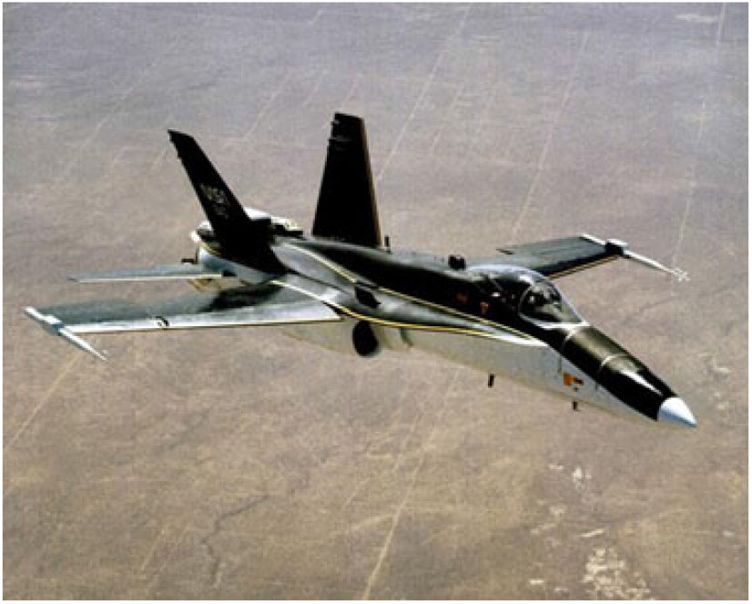
Figure 40. F-18 High Alpha Research Vehicle, HARV.
The F-18 HARV became a new source of experimental information to guide the emerging Navier-Stokes simulation capability of separation-induced vortex flows. Enhanced upwind algorithms coupled with zonal grid approaches for increased geometric realism and efficient grid-point utilisation enabled a rapid leap from the work just discussed with simple delta wings to complex configuration analysis. Ghaffari et al.(Reference Ghaffari, Luckring, Thomas and Bates88) took a novel approach for initiating viscous vortex flow simulations for the F-18 HARV in 1989. The forebody-Leading-edge Extension (LEX) portion of the aircraft was modelled back to the LEX-wing juncture and the vehicle cross section at this station was extended downstream, as a shroud. Longitudinal grid-blocking was used to create a grid of 0.37 m points, and the simulations were performed for both laminar and turbulent flow assumptions using a newly developed longitudinal blocked-grid version of CFL3D. Turbulence was modelled with the physics-based Degani-Schiff(Reference Degani and Schiff89) extension to the Baldwin-Lomax(Reference Baldwin and Lomax90) turbulence model. Figure 41 shows Ghaffari’s F-18 HARV forebody-LEX grid.
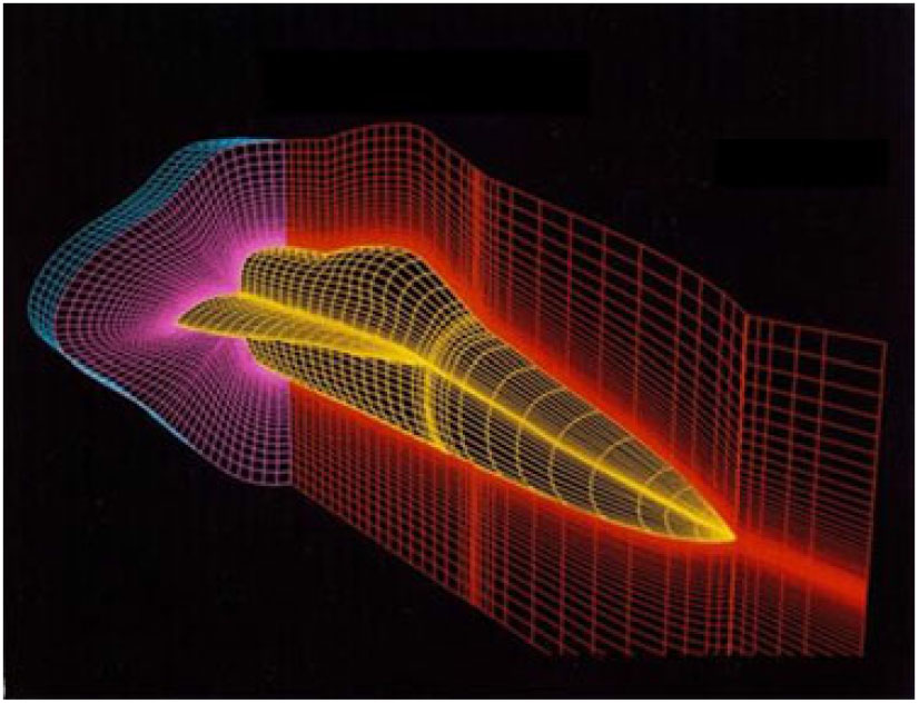
Figure 41. F-18 Forebody-LEX grid. Ghaffari et al.(Reference Ghaffari, Luckring, Thomas and Bates88).

Figure 42. Forebody streamline comparison with flight test, CFL3D. Forebody-LEX CFD model, M = 0.34, Re c = 13.5 × 10⁶, α = 19°. Ghaffari et al.(Reference Ghaffari, Luckring, Thomas and Bates88). (a) Bottom view. (b) Side view.
Correlations between new in-flight surface flow-visualisation and the CFL3D simulations are shown in Fig. 42. The simulations matched flight conditions, and the patterns were surprisingly similar. Effects from the neglected geometry in the simulations appeared to be small, at least to the level of these qualitative comparisons. Further correlations for static surface pressures on the forebody-LEX were made with recent wind-tunnel measurements of a full configuration tested in the David Taylor Model Basin 7-by-10-foot tunnel, and the correlation is shown in Fig. 43. The simulations matched wind-tunnel test conditions, and the predictions of the forebody and forward LEX pressures were surprisingly good. The degraded correlation towards the aft portion was likely associated with the neglected geometry in the CFD simulation. To further understand the forebody-LEX flow, Ghaffari’s numerical shroud extension was fabricated and tested with a forebody-LEX model of the FA-18 in the Langley Research Center (LaRC) Low-Turbulence Pressure Tunnel (LTPT) as briefly discussed in Hall’s(Reference Hall, Murri, Erickson, Fisher, Banks and Lanser86) HATP review. Whereas CFD simulations are usually performed to approximate an experiment, the experiment was performed, in this case, to approximate the CFD simulations.
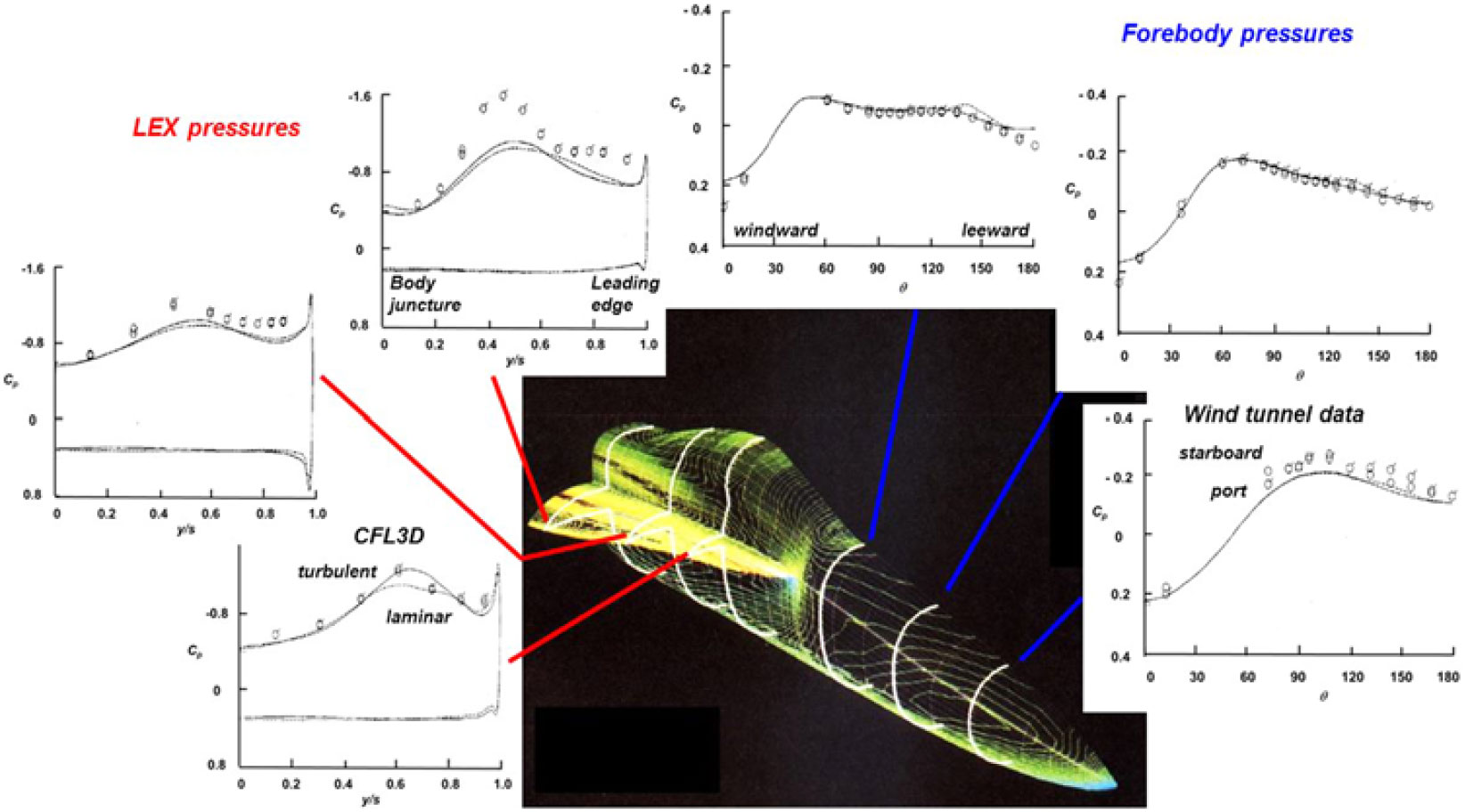
Figure 43. Static surface pressure comparison with wind-tunnel measurements, CFL3D. Forebody-LEX CFD model, M = 0.6, Re c = 0.8 × 10⁶, α = 20°. Ghaffari et al.(Reference Ghaffari, Luckring, Thomas and Bates88).
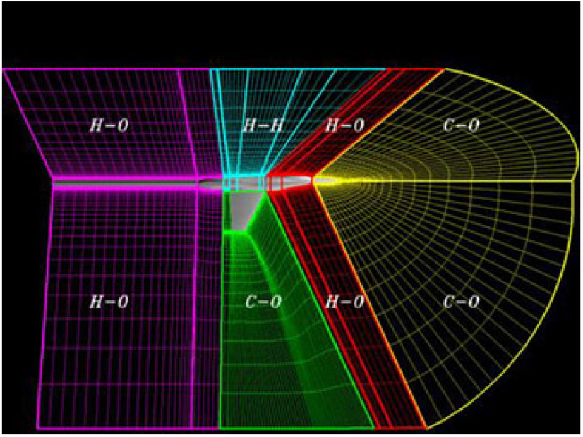
Figure 44. F-18 Forebody-LEX-Wing-Aftbody grid. Ghaffari et al.(Reference Ghaffari, Luckring, Thomas, Bates and Biedron91).
Ghaffari et al.(Reference Ghaffari, Luckring, Thomas, Bates and Biedron91) extended the F-18 HARV analysis in 1991 to include the wing and fuselage. A generalised surface patching capability had been developed with CFL3D, and Ghaffari created a 20-block representation of the HARV geometry with 1.24 m points. Some aircraft components had to be smoothed over, but the representation was otherwise accurate. The modelling excluded the empennage but did include the wing leading-edge flap. Ghaffari’s grid strategy is shown in Fig. 44.
The overall flowfield is shown in Fig. 45 for the configuration with a 25° deflected leading-edge flap and at the same flight conditions from the forebody-LEX studies. This analysis included off-body streamline tracing and crossflow plane total pressure contours. The results show a small forebody vortex as well as the large LEX leading-edge vortex. RANS simulation captured an interaction between these two vortices. The wing has stalled, and the LEX vortex shows vortex breakdown ahead of the wing trailing edge. This breakdown was related to wing trailing-edge pressure recovery.
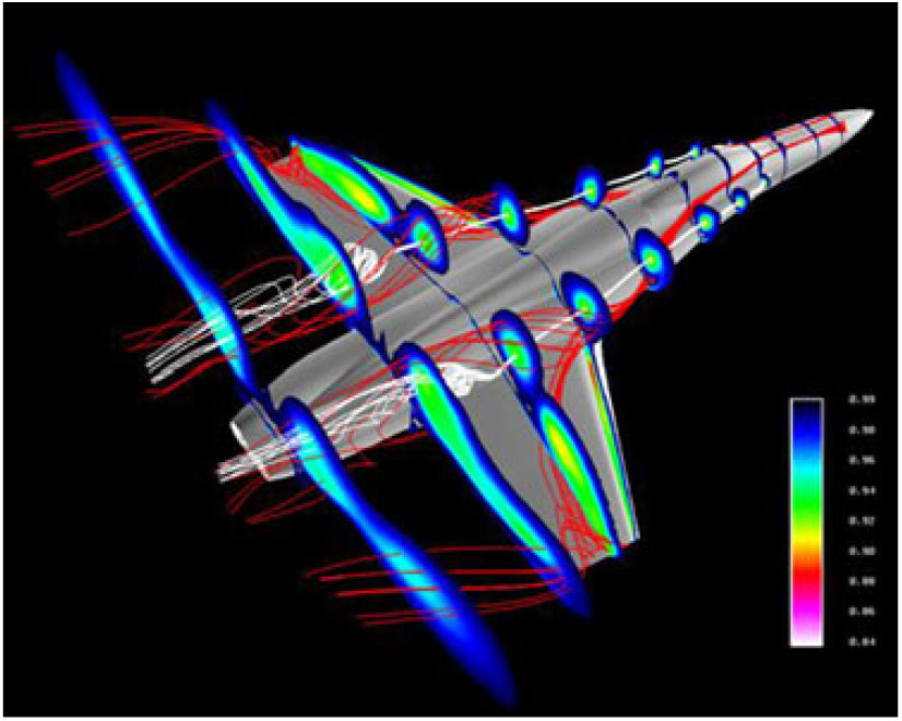
Figure 45. F-18 Forebody-LEX-Wing-Aftbody simulation, CFL3D. M = 0.34, Re c = 13.5 × 10⁶, α = 19°. Ghaffari et al.(Reference Ghaffari, Luckring, Thomas, Bates and Biedron91).
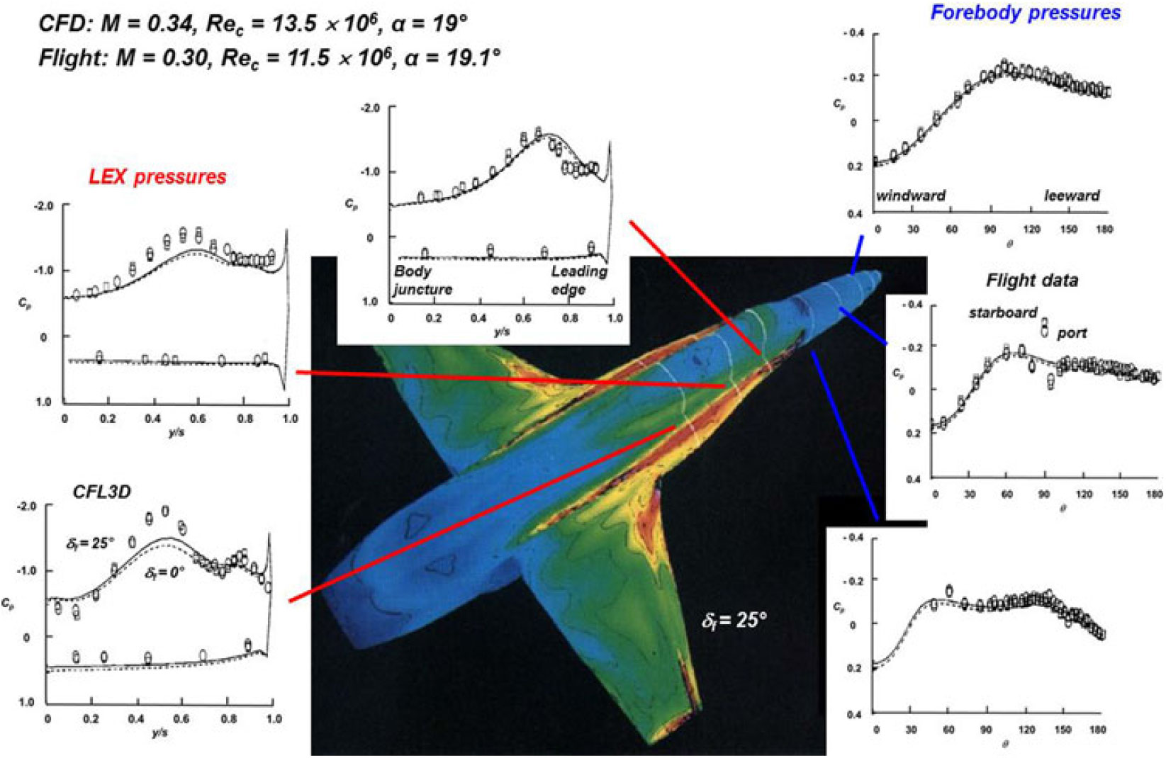
Figure 46. Static surface pressure comparison with flight test, CFL3D. Forebody-LEX-Wing-Aftbody CFD model. Ghaffari et al.(Reference Ghaffari, Luckring, Thomas, Bates and Biedron91).
Correlations with inflight surface pressure measurements are shown in Fig. 46. The CFD corresponds to the flow image in Fig. 45, and the flight data were obtained at slightly different freestream conditions. Correlations for the forebody were very good. A discrepancy was observed at the middle forebody station near θ = 90° and was found to be associated with a blister on the aircraft that was not modelled in the CFD. Pressure correlations on the LEX were good at the first two stations, but at the third station, CFD still underpredicted the primary vortex suction peak. Leading-edge flap deflection from the CFD had only a small effect on these pressures, but this modelling excluded the inboard gap of the deflected leading-edge flap. A current test program for the F/A-18 in the NASA LaRC 7-by-10-foot high-speed tunnel was augmented to assess this gap effect as well as other geometric approximations Ghaffari had made. In general, these effects were found to be small as regards the LEX pressure discrepancy. The contemporary use of experimentation to guide CFD assessments was valuable, and grid resolution effects were one possible source for the discrepancy. Considering Fig. 45, this would include field resolution effects on the interactions between the forebody and LEX vortex systems.
Ghaffari’s work had demonstrated that accurate simulations of viscous vortex flows could be realised for complex configurations, and at flight conditions, with the grid generation and numerical methods of that time for solving the thin-layer Navier-Stokes equations. Other complex-configuration/complex-flow RANS analyses were also being accomplished at this time. For example, in 1988 Flores and Chaderjian(Reference Flores and Chaderjian92) simulated transonic viscous flow about a complete F-16A aircraft configuration, including power effects, at a root-chord Reynolds number of 4.5 m by using a zonal approach with 0.5 m points. Many of these computations were for steady flow and included other compromises to configuration geometry and flowfield grid resolution to fit within the contemporary supercomputer capacity as well as to meet program schedule requirements. Unsteady RANS simulations for vortex flows had been less than fully acceptable. Independent of the vortex research, a new simulation approach was developed to improve unsteady rotational flow simulation based upon a combination of RANS and LES numerical techniques. This hybrid approach will be discussed in the next section.
5.2.2.3 Hybrid RANS/LES analysis
In 1997, Spalart, Jou, Strelets and Allmaras(Reference Spalart, Jou, Strelets and Allmaras93) proposed a hybrid RANS/LES approach for solving time-accurate unsteady flows. This approach combined RANS simulation near the configuration, LES simulation in the field and techniques to interface the two formulations. The LES approach was superior to unsteady RANS for the field simulations, and the RANS approach provided a means to approximate the near-wall flow physics in a manner that would render the hybrid computations tractable within contemporary supercomputer resources. During the 1990s, unstructured flow solver technology had been established and sufficiently matured to provide configuration aerodynamics analysis capability with methods such as the Tetrahedral Unstructured Software System (TetrUSS)(Reference Frink, Pirzadeh, Parikh, Pandya, Bhat and Tetrahedral Unstructured94), amongst others. The marriage of hybrid RANS/LES with unstructured technology was a natural fit, and one approach was developed at the United States Airforce Academy and embodied in a program known as Cobalt(Reference Strang, Tomaro and Grismer95). Analysis for this section will be for the numerical solution of viscous rotational flows that are unsteady.
Vortex breakdown is one important vortex flow phenomenon with unsteady content, and Morton et al.(Reference Morton, Forsythe, Mitchell and Hajek96) assessed predictions from hybrid RANS/LES with the Cobalt code in 2002. The formulation used the Spalart-Allmaras (SA)(Reference Spalart and Allmaras97) turbulence model in the RANS portion and Detached Eddy Simulation (DES) for coupling to the LES portion. The study focused on a 70° delta wing tested by Mitchel et al.(Reference Mitchell, Molton, Barberis and Delery98) as part of a larger vortex breakdown study(99) facilitated through the NATO Research and Technology OrganizationFootnote 5 (RTO). Unstructured grids of approximately 2.5 m cells were used for the simulation, and a sample result is shown in Fig. 47. For the conditions chosen, bursting occurred over the wing around 60% root chord, and a time-accurate trace of the predicted burst location is compared to bounds observed experimentally. The experiment was at a slightly higher angle-of-attack due to wall interference effects, which could account for some of the offset between the experimental mean and the computed result. Vortex breakdown is still very difficult to predict at the time of this writing, and the correlation shown by Morton was an encouraging accomplishment. Morton included numerical assessments of the hybrid formulation, grid assessments and comparisons with RANS formulations as part of his study.
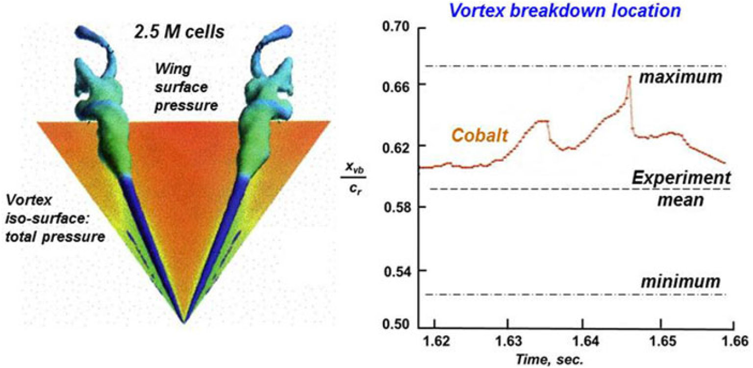
Figure 47. Hybrid RANS/LES delta wing simulation, Cobalt. Λ = 70°, M = 0.07, Re cr = 1.56 × 10⁶, α = 27°. Morton et al.(Reference Morton, Forsythe, Mitchell and Hajek96).
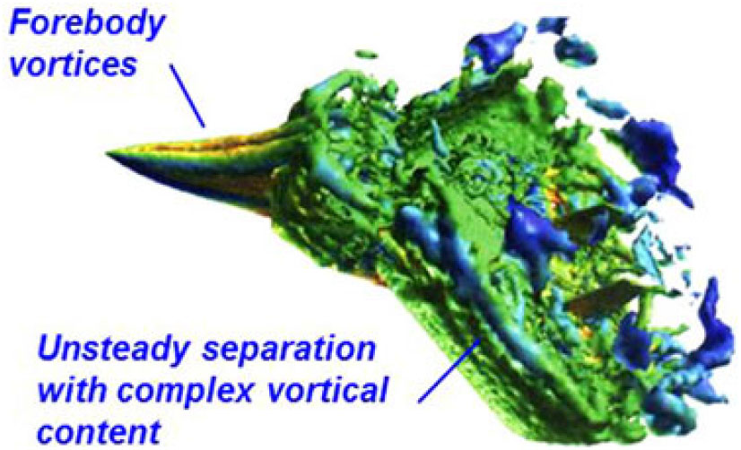
Figure 48. Hybrid RANS/LES simulation, Cobalt. F-15E, M = 0.3, Re c = 13.6 × 10⁶, α = 65°.
Forsythe et al.(Reference Forsythe, Squires, Wurtzler and Spalart100).
In a manner similar to the RANS analysis evolution discussed in section 5.B.2.b., a rapid leap of the hybrid RANS/LES technology occurred from simple to complex configuration analysis. In 2002, Forsythe et al.(Reference Forsythe, Squires, Wurtzler and Spalart100) demonstrated hybrid RANS/LES computations about a full F-15E configuration at a very high angle-of-attack of 65° and a flight Reynolds number of 13.6 × 10⁶. The computations used the same SA/DES formulation just discussed. Mesh sensitivity studies ranged from 2.9 m to 10 m cells, and their baseline grid was comprised of 5.9 m cells. The flow simulation is shown in Fig. 48. The forebody vortices remained coherent with small-scale unsteadiness despite this very high angle-of-attack. The wing demonstrated unsteady separation with complex vortical content. Vortical structures that shed from the leading edge became incoherent as they progressed over the wing planform.
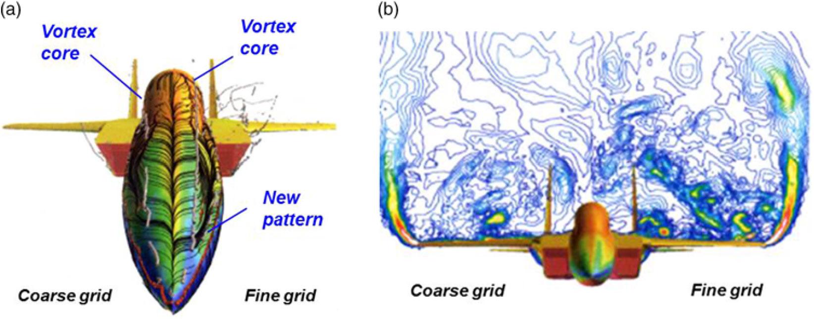
Figure 49. Grid resolution effects, Cobalt. F-15E, M = 0.3, Re c = 13.6 × 10⁶, α = 65°. Forsythe et al.(Reference Forsythe, Squires, Wurtzler and Spalart100). (a) Forebody. (b) Wing.
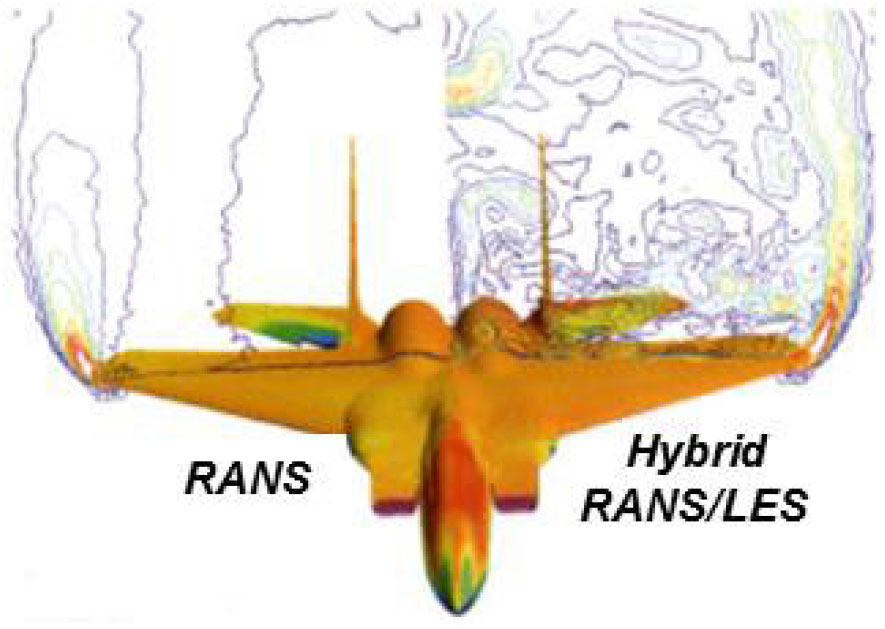
Figure 50. Governing equations effect, Cobalt. F-15E, M = 0.3, Re c = 13.6 × 10⁶, a = 65°.
Forsythe et al.(Reference Forsythe, Squires, Wurtzler and Spalart100).
An example of the mesh resolution effects is shown in Fig. 49. Forsythe’s fine grid produced a more coherent forebody vortex with a new surface flow pattern inboard of primary separation. The fine grid also altered the forebody vortex trajectory from going around the canopy to going over the canopy. The instantaneous flowfield cut over the wing demonstrated the increased vorticity resolution achieved with the fine grid. Much of this fine-grid content was absent in the coarse-grid simulation, and this demonstrated the feature resolving capacity of this formulation with the finer grid.
Forsythe also compared RANS and hybrid RANS/LES simulations. The same grid and turbulence model (Spalart-Allmaras) was used for both simulations. His unsteady RANS (URANS) computations did not exhibit any significant unsteadiness and were equivalent to steady RANS computations. A comparison of his URANS and hybrid RANS/LES results is shown in Fig. 50. The cut over the wing shows instantaneous vorticity contours and clearly demonstrates the feature resolving capacity of the hybrid RANS/LES approach. The RANS solution has virtually no vorticity content over the wing at this very high angle-of-attack. Forsythe also reported that the hybrid RANS/LES computations correlated better with flight test forces and moments than the RANS results.
The hybrid RANS/LES formulation had demonstrated a significant advancement in resolving complex vortical flows as compared to RANS formulations. The detailed vortical features could be captured by the LES portion of the solver but were limited to the accuracy of the underlying grid. Adaptive grid techniques are particularly well suited for unstructured grids, and the extension of hybrid RANS/LES capability to include Adaptive Mesh Refinement (AMR) with unstructured grids offered an attractive means to further exploit the feature resolving capacity of hybrid RANS/LES technology while maintaining some control over problem size (i.e., cell count).
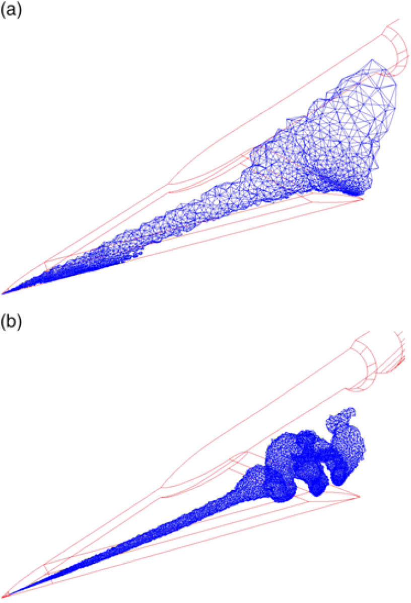
Figure 51. Adaptive grid result, inviscid flow, USM3D. Delta wing, sharp leading edge, M = 0.4, α = 20°. Pirzadeh.(Reference Pirzadeh101). (a) Unadapted grid. (b) Adapted grid.

Figure 52. Adaptive grid result, viscous flow, USM3D. Delta wing, blunt leading edge, x/c r = 0.5, M = 0.4, Re mac = 6 × 10⁶, α=20°. Pirzadeh.(Reference Pirzadeh101). (a) Unadapted grid. (b) Partially adapted grid.
A promising adaptive grid approach for separation-induced leading-edge vortex flow simulations was demonstrated at an RTO symposium by Pirzadeh(Reference Pirzadeh101) in 2001, one year before the Morton et al.(Reference Morton, Forsythe, Mitchell and Hajek96) delta wing work discussed with Fig. 47. Pirzadeh’s work was based on Euler and RANS analyses using the TetrUSS flow solver USM3D at moderate angles of attack that would produce concentrated leading-edge vortices but that could include vortex breakdown. His grid adaptation was based upon entropy production in the field, and the adaptation resulted in significant improvements in leading-edge vortex resolutions for both the vortex sheet and the vortex core. An example of vortex core resolution is shown in Fig. 51 for an inviscid Euler simulation about a sharp-edge delta wing geometry tested at NASA LaRC by Chu and Luckring(Reference Chu and Luckring102). The unadapted case followed standard grid generation practices that resulted in 0.4 m cells. Adaptive grid refinement produced 1.6 m cells and a greatly improved resolution of the vortex core, as shown in Fig. 51(b). Surface grid refinement was also included in this approach, and refined surface pressures were shown.
Pirzadeh also demonstrated this technique for viscous vortex flow, as seen in Fig. 52. The TetrUSS system produces a near-body viscous grid of advancing layers that couples with an unstructured tetrahedral field grid. Pirzadeh’s adaptation was restricted to the field grid, and he referred to the viscous adaption process as partially adapted grids. An example of his results is shown in Fig. 52 for the delta wing just discussed but with a blunt leading edge (r le/mac = 0.15%). This example demonstrates significantly improved grid resolution of the vortex sheet by the adaptive grid technology. The unadapted grid had 1.7m cells, whereas the adapted grid had 4m cells. The adaptive grid results also resulted in a shift in the primary vortex and secondary separation locations, and this solution correlated better with experiment than did the unadapted solution. An assessment of his adaptive grid technique for a vortex interaction case with dual primary vortices from a chine-wing configuration due to Hall(Reference Hall103) was also included. Pirzadeh’s initial work was not fully automated, and there was no effort to manage the total problem size, such as with grid derefinement. Nonetheless, his results demonstrated effective unstructured grid adaptation to the leading-edge vortex flows.
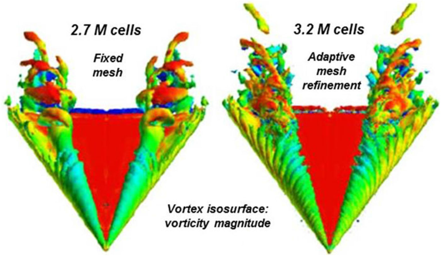
Figure 53. Hybrid RANS/LES delta wing simulation, adaptive mesh refinement, Cobalt. Λ = 70°, M = 0.07, Re cr = 1.56 × 10⁶, α = 27°. Morton et al.(Reference Morton, Steenman, Cummings and Forsythe105).
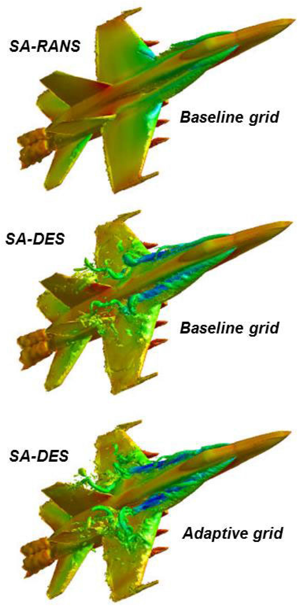
Figure 54. Hybrid RANS/LES simulations, Cobalt. F-18C, M = 0.28, Re cref = 13.9 × 10⁶, α = 30°.
Morton et al.(Reference Morton, Steenman, Cummings and Forsythe105).
Mitchel et al.(Reference Mitchell, Morton and Forsythe104) used Pirzadeh’s approach with hybrid RANS/LES simulations of vortex flows with adapted grids in 2002. This was the first coupling of an adaptive mesh with a hybrid RANS/LES simulation. The approach for hybrid RANS/LES simulations of vortex flows with adaptive mesh refinement was further assessed by Morton et al.(Reference Morton, Steenman, Cummings and Forsythe105) in 2003. The computations were performed with Cobalt and the same SA/DES formulation mentioned above, and field adaptation was now based on vorticity. The application was for the 70° delta wing used previously for vortex breakdown studies (Fig. 47) at the same flow conditions, and a sample result is shown in Fig. 53. An unadapted solution with 2.7m cells was contrasted with the adaptive-grid result. The adaptive grid result showed significantly improved resolution of vortical substructures within the primary vortex sheet as well as finer detail in the burst region of the vortex. The adaptive solution only resulted in 3.2m cells, a 19% increase in total cell count compared to the unadapted computation.
Morton et al.(Reference Morton, Steenman, Cummings and Forsythe105) also demonstrated in 2003 an application of this technology to the F-18C at full-scale flight conditions and a high angle-of-attack of 30°. The study included flow simulations from steady and unsteady RANS, from hybrid RANS/LES, and from hybrid RANS/LES with adaptive mesh refinement. Both the RANS and hybrid RANS/LES solutions used 5.9m cells, and the adaptive grid solution resulted in 6.2m cells (a 5% increase). Results are shown in Fig. 54 for an instantaneous view of vorticity isosurfaces coloured by pressure. The F-18C wing is stalled at the angle-of-attack studied, and some incoherent vorticity is captured by the hybrid RANS/LES formulation. The RANS simulation failed to capture this effect, similar to the F-15E very high angle-of-attack study by Forsythe(Reference Forsythe, Squires, Wurtzler and Spalart100). The hybrid RANS/LES solutions showed more vortical content over the leading-edge extension (LEX) than the RANS solutions, and the adaptive mesh refinement showed increased vortical resolution consistent to the delta wing studies mentioned above. Both hybrid RANS/LES flow patterns also indicated possible vortex breakdown of the LEX vortex over the wing.
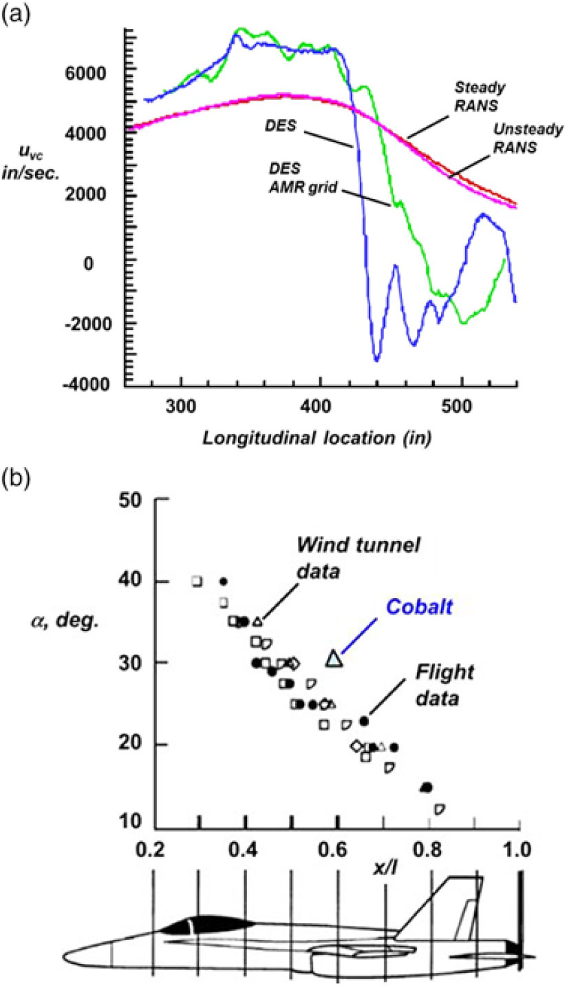
Figure 55. Hybrid RANS/LES simulation, Cobalt. F-18C, M = 0.28, Re cref = 13.9 × 10⁶, α = 30°. Data, various sources. Morton(Reference Morton, Steenman, Cummings and Forsythe105). (a) LEX vortex core longitudinal velocity. (b) Vortex breakdown location.
Vortex breakdown analysis was performed on these solutions, and an example is shown in Fig. 55. The longitudinal velocity along the centre of the vortex core, uvc, was chosen as the vortex breakdown metric with a negative value indicating vortex breakdown. RANS failed to predict vortex breakdown whereas both hybrid RANS/LES solutions did. The prediction was further downstream than experimental results(Reference Fisher, Del Frate and Zuniga106) from the F-18 HARV, and the authors attributed this to the absence of the diverter slot on the F-18 HARV.
These results demonstrated that the hybrid RANS/LES with AMR could resolve vortex flow physics that could otherwise be missed without the combined technology. They also demonstrated that the technique could be applied to complex configurations with complex vortical flows.
The examples provided thus far have focused on vortices separating from sharp edges. However, in many applications, the leading-edge vortices will occur on wings with blunt leading edges, and bluntness fundamentally alters the separation-induced vortical flows. This class of leading-edge vortex separation will be discussed in the next section.
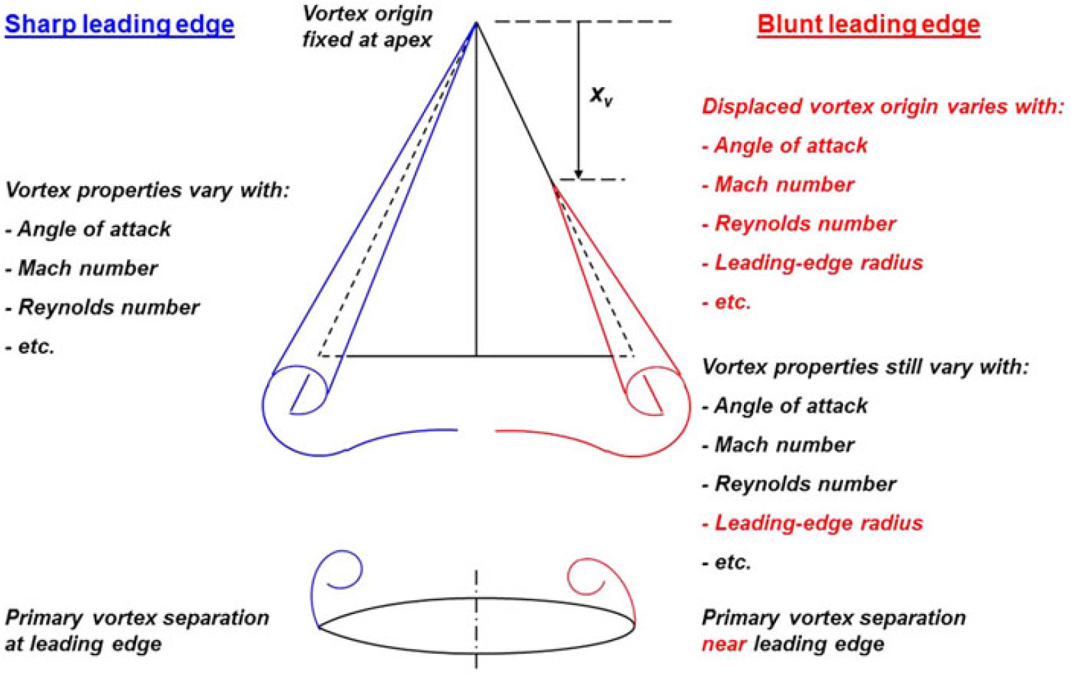
Figure 56. Blunt-leading-edge vortex separation. Luckring(Reference Luckring107).
5.3 Three-dimensional flows, blunt-leading-edge vortices, single primary vortex
Some fundamental flow physics for separation-induced leading-edge vortices for a 65° delta wing with blunt leading edges were described by Luckring(Reference Luckring107) in 2004. The discussion was based upon an experimental program conducted in the NASA Langley National Transonic Facility (NTF) in the early 1990s as reported by Chu and Luckring(Reference Chu and Luckring102) in 1996. A sketch from Luckring(Reference Luckring107) contrasting sharp and blunt-leading-edge vortex separation for delta wings is shown in Fig. 56. The left semi-span of the delta wing shows the sharp-edged case with the origin of the vortex at the apex of the delta wing and vortex separation fixed at the sharp leading edge. The right semi-span shows the blunt-edged case where the origin of the vortex is displaced from the apex of the delta wing. This vortex origin varies with angle-of-attack, Mach number, Reynolds number and leading-edge radius, amongst other effects (camber, surface roughness, etc.) In addition, the vortex separation will now occur near, but not necessarily at, the leading edge. The blunt leading edge introduces many effects not present for the sharp-edged case.
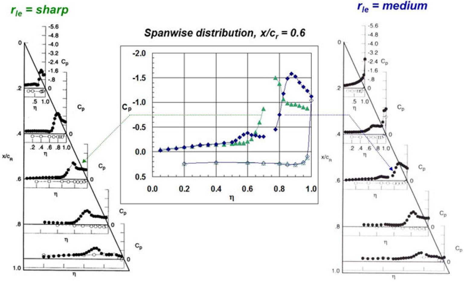
Figure 57. Blunt-leading-edge vortex separation, spanwise pressure distributions. Delta wing, Λle = 65°, M = 0.4, Re mac = 6 × 10⁶, a = 13.3°. Luckring(Reference Luckring108).
One set of results from Luckring’s experiment is shown in Fig. 57. Spanwise surface pressure measurements are contrasted between the wing with a sharp leading edge and the wing with a blunt leading edge. The sharp-edged case shows leading-edge vortex separation at all pressure stations, whereas the blunt-leading-edged case shows attached flow near the wing apex and vortex flow for the aft portion. The blunt leading-edge surface pressures showed a curious bubble-like pressure distribution near the leading edge at the 40% chord station as well as an unanticipated inboard suction peak at the 60% chord station. Discovery of these unusual pressure characteristics from the NTF experiment served as an impetus for new collaborations to study the blunt-leading-edge vortex flows.
Two collaborative programs were executed to obtain new data and develop predictive capability for separation-induced vortex flows from blunt leading edges. Both programs were facilitated through the NATO Applied Vehicle Technology Program (AVT) Research and Technology Organization (RTO), later renamed the Science and Technology Organization (STO). This work focused on delta and diamond wing configurations, Fig. 58.
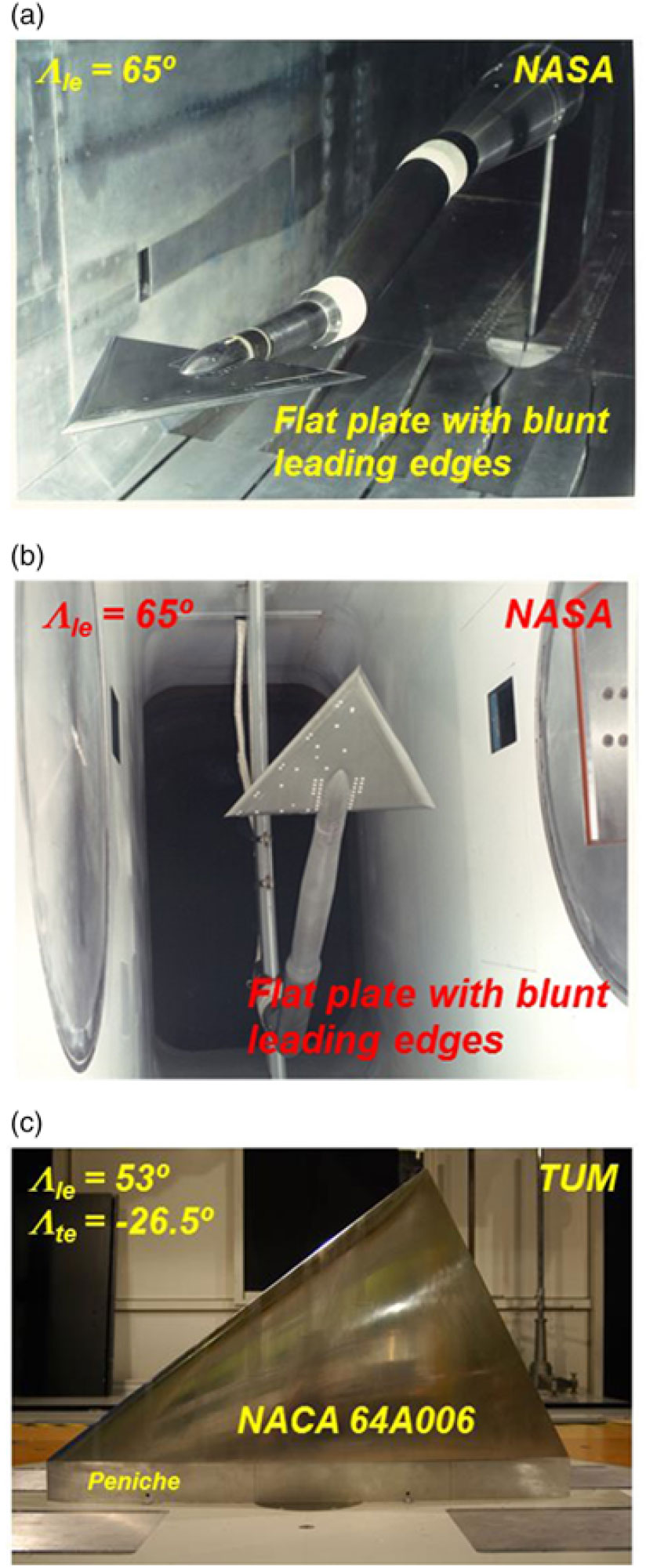
Figure 58. New experiments, blunt-leading-edge vortex separation. (a) Delta wing, NTF. (b) 0.75-scale delta wing, LTPT. (c) Diamond wing, TUM.
The first program was organised under the NATO Task Group AVT-113(109) and became known as Vortex Flow Experiment 2 (VFE-2). The work was anchored in the NTF delta wing results just described, and the 0.75-scale delta wing model was provided to Europe to support further experimentation. Four additional models were fabricated, and 15 new wind-tunnel tests were accomplished throughout Europe along with CFD analysis from eight different codes. This project ran from 2003 to 2008 with participation from 12 institutions spanning seven countries.
The second program was organised under the NATO Task Group AVT-183(110). The work focused on a diamond wing that was designed to isolate blunt-leading-edge vortex separation in a manner relevant to challenges discovered on an Uninhabited Combat Air Vehicle (UCAV) configuration of interest to another NATO Task Group, AVT-161(111). A new wind-tunnel model was fabricated, and three new wind-tunnel tests were accomplished at the Technische Universität München (TUM), Germany. In addition, CFD analysis was accomplished with 11 different codes. This project ran from 2010 to 2016 with participation from 13 institutions spanning six countries.
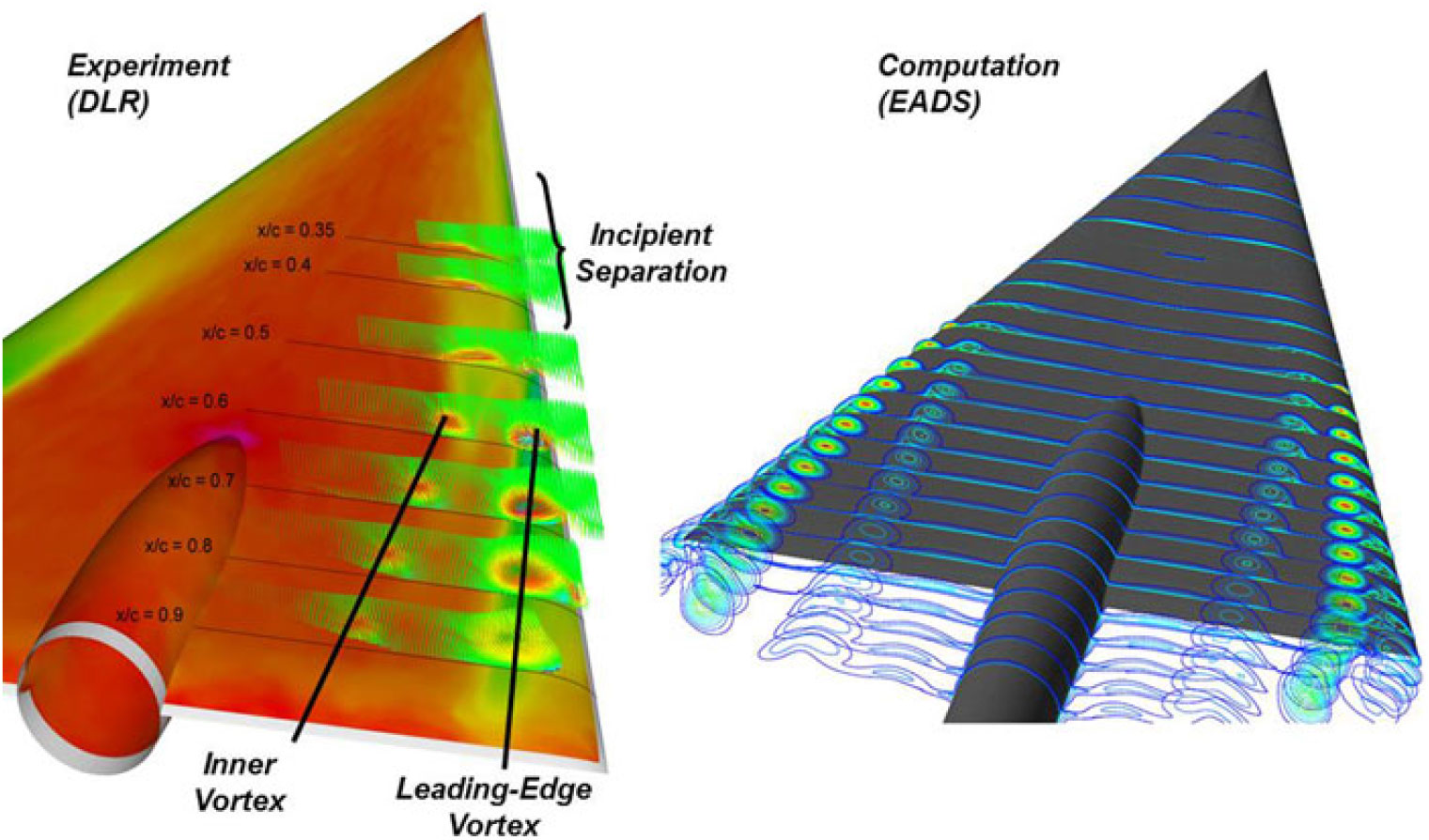
Figure 59. Blunt-leading-edge vortex separation, spanwise pressure distributions. Delta wing, Λle = 65°, M = 0.4, Re mac = 6 × 10⁶, α = 13.3°. Luckring and Hummel(Reference Luckring and Hummel112).

Figure 60. Insipient vortex separation, USM3D. Diamond wing, Λle = 53°, M = 0.15, Re mac = 2.7 ×10⁶, α = 12°. Frink et al.(Reference Frink, Tomac and Rizzi116).
A highlight from the NATO work in VFE-2 is shown in Fig. 59. Results are at a focus condition for this research and discussed with Fig. 59 from Luckring and Hummel(Reference Luckring and Hummel112). The left portion of Fig. 59 combines experimental results in the form of surface pressure sensitive paints and off-body flowfields from particle image velocimetry by Konrath et al.(Reference Konrath, Klein and Schröder113). These results were obtained at the German Aerospace Center (DLR) in Germany. The measurements clearly indicated the presence of an inner vortex with the same sense of rotation as the leading-edge vortex. The inner vortex appeared to have its origin in the incipient separation region, although the details of this separation process were unclear. The right portion of Fig. 59 shows the first successful numerical simulation of the blunt-leading-edge vortex separation at the focus condition of VFE-2. These computations were performed by Fritz(Reference Fritz114) using the DLR FLOWer code(Reference Kroll, Aumann, Bartelheimer, Bleecke, Eisfeld, Lieser, Heinrich, Kuntz, Monsen, Raddatz, Reisch and Roll115) and demonstrated good qualitative agreement with experiment.
A clearer view of the incipient separation region was produced by Frink et al.(Reference Frink, Tomac and Rizzi116) as part of the AVT-183 diamond-wing research project, as seen in Fig. 60. Frink’s results demonstrated a clear demarcation in the incipient separation region of surface streamlines that remained inboard on the attached-flow portion of the wing from those outboard, near the leading edge, that became entrained into the nascent blunt-leading-edge vortex. His solution also showed the inner vortex, which appeared to have its origin near the kink in the streamlines separating the inner wing flow from the outer blunt-leading-edge vortex flow.

Figure 61. Inner vortex separation. Diamond wing, Λle = 53°, M = 0.15, Re mac = 2.7 × 10⁶, α = 12°. Hitzel et al.(Reference Hitzel, Boelens, Rooij and Hövelmann117).
An explanation for the origin of the inner vortex was first given by Hitzel et al.(Reference Hitzel, Boelens, Rooij and Hövelmann117), also as part of the AVT-183 diamond-wing research project. A modified version of Hitzel’s figure for this explanation is shown in Fig. 61. This figure has many details of the blunt-leading-edge vortex flow, and those associated with the inner vortex formation are highlighted. Hitzel observed that, for the blunt-leading-edge wing, the fully attached flow from the inboard and upstream portion of the wing would turn spanwise in the outboard direction as it progressed downstream due to the basic pressure field of a slender wing with attached flow. The leading-edge vortex induces reattachment of the flow on the upper surface of the wing. In the outboard of reattachment, the flow is induced in the outboard direction under the vortex, and the inboard of reattachment flow is induced in the inboard direction over the wing. By Hitzel’s analysis, the confluent outward-flowing and inward-flowing boundary layers result in the formation of the inner vortex. The inner vortex is thus a consequence of the attached flow from the inboard and upstream blunt leading edge interacting with the flow induced by the blunt-leading-edge vortex.

Figure 62. Effect of insipient separation location on correlation, KESTREL. Diamond wing, Λle = 53°, 6ptM = 0.15, Re mac = 2.7 × 10⁶. Daniel et al.(Reference Daniel, Malloy, Reasor and Morris118).
Extensive correlations between CFD and experiment were performed in the AVT-183 project, and the prediction of the incipient separation region was found to be crucial to the overall agreement. An example is shown in Fig. 62 from Daniel et al.(Reference Daniel, Malloy, Reasor and Morris118), with CFD predictions from the Kestrel code(Reference Morton, McDaniel, Sears, Tillman and Tuckey119) and experimental results from Hoevelmann(Reference Hövelmann, Knoth and Breitsamter120, Reference Hövelmann, Grawunder, Buzica and Breitsamter121). The left portion is an example where the incipient separation matched between computation and experiment, and the correlation is very good for the entire wing. The right portion is for a lower angle-of-attack where the prediction of incipient separation did not match the experimental location, and the correlation of wing pressures is degraded, especially as regards to the leading-edge vortex effects. Between the AVT-113/VFE-2 and the AVT-183 research programs, the successful prediction of a blunt-leading-edge vortical flow was accomplished so long as a single phenomenon, the onset of the blunt-leading-edge vortex separation, matched. This incipient separation has now been identified as the remaining critical factor for successful predictions. The detailed physics of the incipient separation, as well as the progression of the incipient separation with angle-of-attack, remain to be fully understood. Many additional details of the blunt-leading-edge vortex research can be found in special issues of Aerospace Science and Technology for AVT-113/VFE-2(Reference Hövelmann, Grawunder, Buzica and Breitsamter121) and AVT-183(Reference Cummings and Ghoreyshi123).
The examples provided thus far have focused on vortical flows with a single primary vortex system (with associated secondary and inner vortices). However, many applications can result in multiple primary vortex systems being formed, often associated with wing geometric features, and the interactions between the primary vortices present another class of vortical flow physics. This class of leading-edge vortex flow will be discussed in the next section.
5.4 Three-dimensional flows, sharp or blunt-leading-edge vortices, multiple interacting vortices
Three fundamental classes of vortex interactions are chosen for discussion. The first is the interaction between two primary and co-rotating vortex systems, such as would be generated by a double delta wing (vortex-vortex interactions). The second is the interaction between a primary vortex system and a shock (vortex-shock interactions). The third is the interaction between a primary vortex and a surface (vortex-surface interactions). The vortex-surface interactions would include both the interactions between the primary vortex and the underlying wing that results in a secondary vortex as well as the interactions of the primary vortex with a downstream component, such as the empennage. Each class of vortex interaction has its own challenges, and each vortex interaction class can include abrupt state changes (such as from a weak to a strong interaction). Vortex interactions will be discussed in terms of a unique flight-test program, initiated by NASA, along with subsequent international programs focused on computational analysis of the flight data with CFD.
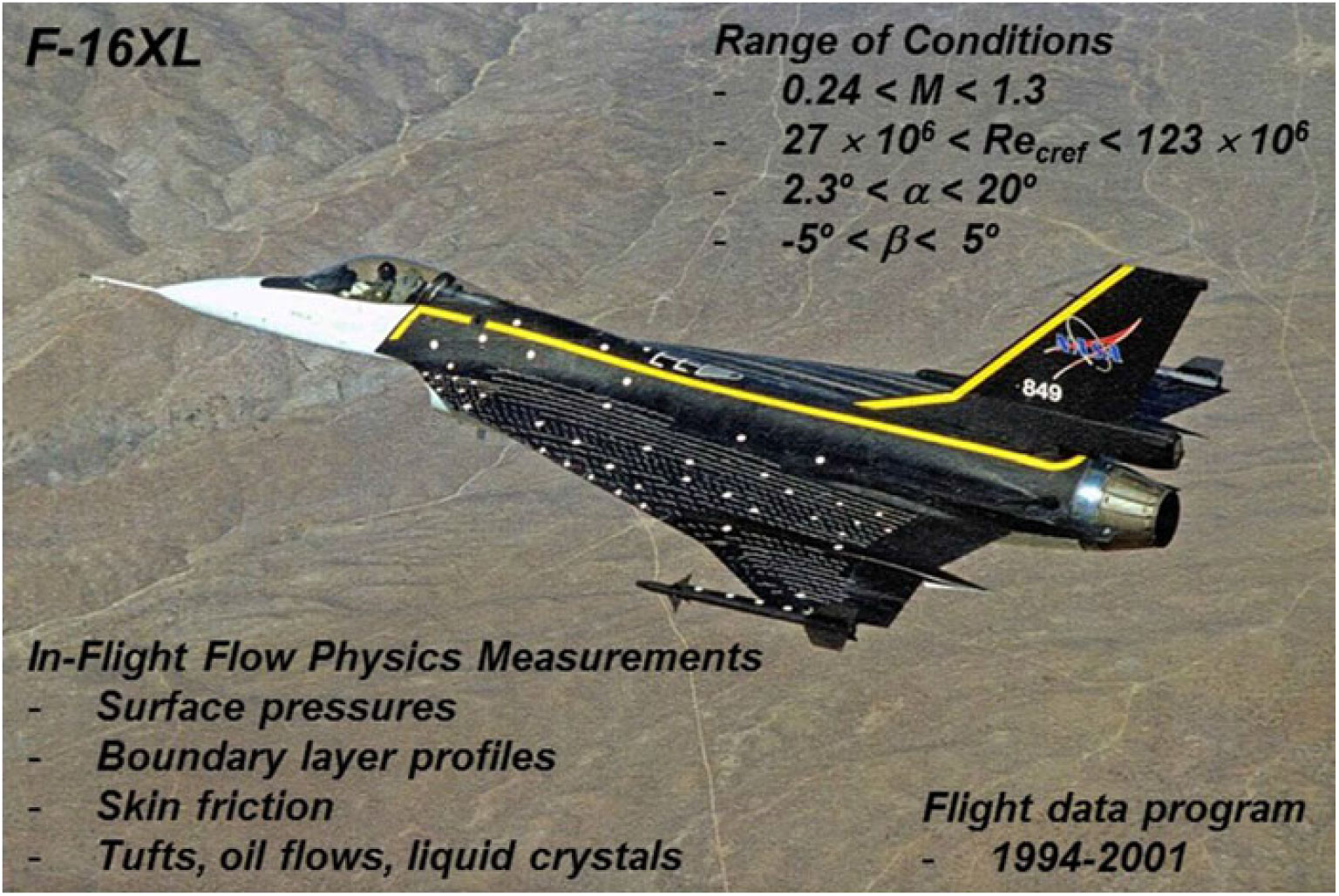
Figure 63. Cranked Arrow Wing Aerodynamics Program, CAWAP.
In the 1990s, NASA conducted a flight-test program to study wing aerodynamics with a General Dynamics F-16XL aircraft. This aircraft has a highly swept wing, designed for efficient supersonic cruise, with a cranked leading edge. The program was known as the Cranked Arrow Wing Aerodynamics Program (CAWAP) and focused on obtaining wing data over a broad range of operating conditions, as seen in Fig. 63. The program was unique in that a number of flow physics measurements were obtained that are uncommon for flight testing. The scope of the test program was reported by Lamar(Reference Lamar, Obara, Fisher and Fisher124) in 2001. Initial correlations between CFD and flight test were reported by Lamar(Reference Lamar125) at an RTO symposium in 2001, and these correlations were, in general, less than acceptable. Although not explicitly discussed as vortex interactions at the time of the work, many of the challenges for predicting the vortex flow aerodynamics of the F-16XL included all three classes of vortex interaction just mentioned. Vortex-vortex interactions occurred due to the cranked leading edge and vortex-shock interactions occurred at the transonic and supersonic test conditions. Vortex-surface interactions occurred in terms of the wing primary vortex inducing not only secondary vortices but also an additional vortex from the edge of a downstream wing component known as an air dam.
A succession of three international programs was executed to seek improved CFD predictive capability of the F-16XL vortex flow aerodynamics on the full-scale airframe at full-scale flight conditions. Collectively, the work ran from 2004 to 2015 with CFD analysis from 12 different codes that was contributed from ten institutions spanning five countries.
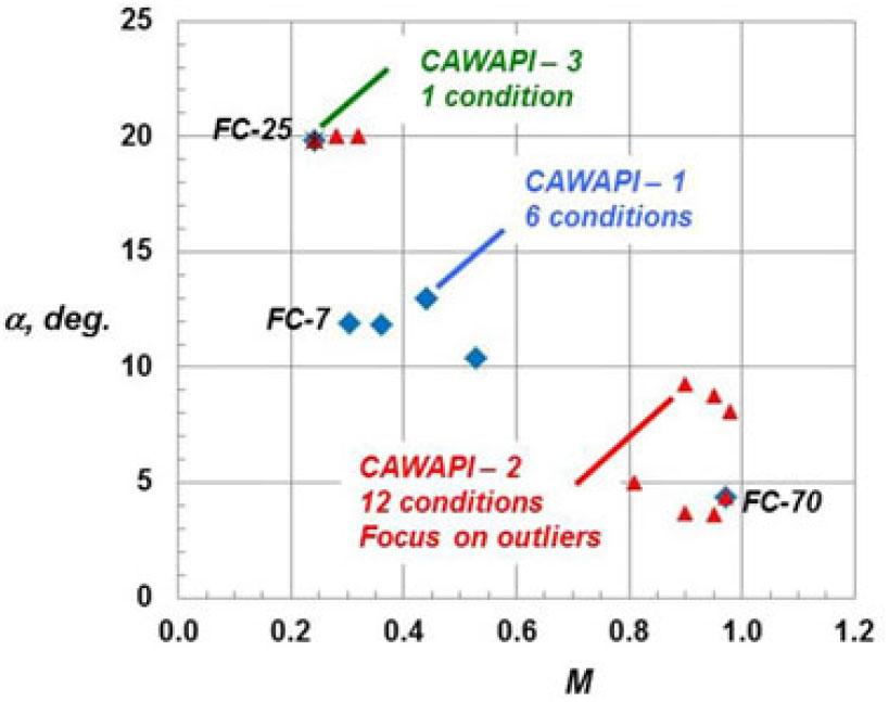
Figure 64. Cranked Arrow Wing Aerodynamics Program, International (CAWAPI) investigations. Luckring et al.(Reference Luckring, Rizzi and Davis126).
The first of these was named CAWAPI (Cranked Arrow Wing Aerodynamics Program International) and was performed as part of the RTO Task Group AVT-113 in conjunction with the VFE-2 work mentioned in Section 5.3. This program focused on six flight conditions as shown in Fig. 64. Four were at moderate angles of attack and moderate Mach numbers, one was at a low-speed high angle-of-attack condition (Flight Condition FC-25), and the last was at a low angle-of-attack and high transonic Mach number (FC-70). The CAWAPI-2 and CAWAPI-3 analysis conditions are also shown in Fig. 64 and will be discussed later in this section. CAWAPI CFD analysis was accomplished using ten different codes with participation from nine institutions spanning five countries. This program ran from 2004 to 2008.
Most of the CAWAPIork focused on the moderate angle-of-attack, moderate Mach number conditions, and, in particular, Flight Condition FC-7. (See, Fig. 64). Sample results are shown in Fig. 65, and at these conditions, the wing vortex flow exhibits, for the most part, weak vortex-vortex interactions. Primary and secondary vortex systems were developed on both the inner and outer wing panels that remain far apart from each other. The secondary vortex from the inboard leading-edge vortex can be observed in Fig. 65(a).
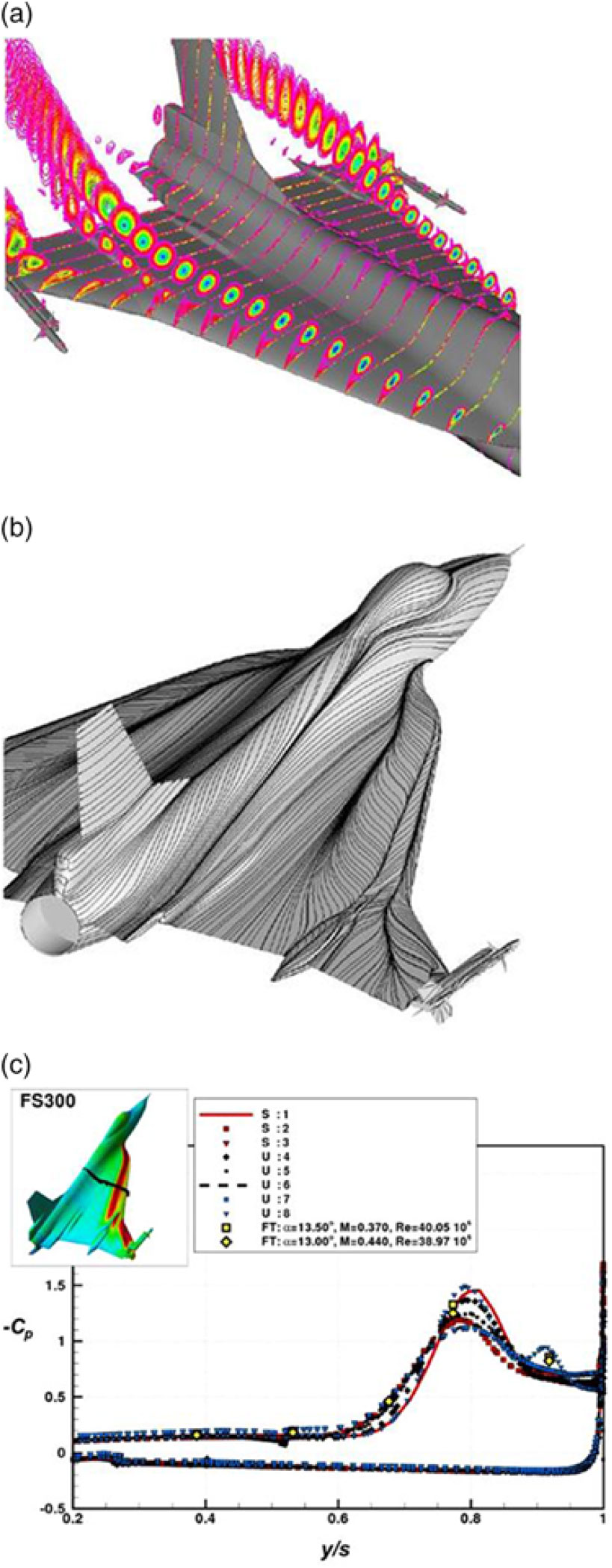
Figure 65. CAWAPI accomplishment. Weak vortex-vortex interactions. FC – 7: M = 0.304, Re cref = 44.4 × 10⁶, α = 11.9°. Rizzi et.al.(Reference Rizzi, Badcock, Jirásek and Boelens127). (a) Off-body vortices. (b) Surface flow pattern. (c) Spanwise pressure predictions.
Supercomputer capacity grew over the course of the CAWAPI investigations, and improved fidelity of F-16XL surface modelling as well as the increased field resolution from the higher grid densities contributed to better resolved flows about the aircraft. Lamar’s(Reference Lamar125) initial CFD work used approximately 1.4m cells, and the median grid amongst the CAWAPI analyses used 15 m cells.
Two examples of CAWAPI flowfield resolution are shown in Fig. 65(a) and (b). (Additional details for these images can be found in Boelens et al.(Reference Boelens, Spekreijse, Sytsma and de Cock128).) This, along with other modelling considerations, led to good correlations amongst the CFD and with flight test data at this moderate condition. An example is shown in Fig. 65(c) where the solutions are presented only as a collective without distinguishing the details amongst the individual simulations. Flight test data are included in this comparison. From the overall CAWAPI effort, a number of the moderate-alpha, moderate-Mach conditions appeared to be much better understood than what was known at the beginning of the program, and it appeared that the weak vortex-vortex interactions could be fairly well simulated on an aircraft geometry at flight conditions (and, in particular, at flight Reynolds numbers). A summary of the CAWAPI findings was published in 2009 in a special section of the American Institute of Aeronautics and Astronautics (AIAA) Journal of Aircraft with an introduction to the special section by Lamar(Reference Lamar129). Most of the CAWAPI analysis was performed with RANS simulations for steady flow.
The CAWAPI work also identified two of the flight conditions that were not well predicted by all participants and warranted further investigation. These became the focus of the CAWAPI-2 effort.

Figure 66. Complex vortex interactions for CAWAPI-2 and CAWAPI-3 studies. (a) Transonic vortex-shock interactions. FC – 70: M = 0.97, Re cref = 89 × 106, α = 4°. Davis(Reference Davis, Reed and Yagle130). (b) Low-speed strong vortex-vortex interactions. FC – 25: M = 0.24, Re cref = 32 × 106, α = 19.8°. Boelens. Included in Luckring et al.(Reference Luckring, Rizzi and Davis126).
The second international program, CAWAPI-2, focused on the two outlier conditions from the CAWAPI work. These conditions were (i) FC-70, the transonic low-alpha case and (ii) FC-25, the subsonic high-alpha case. CFD flowfield simulations for these two conditions are shown in Fig. 66. The transonic case shows a succession of vortex-shock interactions. The low-speed case shows a much stronger vortex-vortex interaction condition on the outboard panel amongst the inboard leading-edge vortex system, a counter-rotating air-dam vortex, and the outboard leading-edge system vortex. Additional flight test data were identified in the neighbourhood of these two extreme conditions to provide additional insights to the complex flows for the CAWAPI-2 work. (See, Fig. 64). CFD analysis was accomplished using four different codes with participation from four institutions spanning four countries. This program ran from 2010 to 2014.
The CAWAPI-2 work addressed aircraft geometric effects (static aeroelastic deflection, control surface deflections and gaps) as well as flow modelling effects (grid resolution, turbulence modelling, unsteady vortex flows). Sustained supercomputer growth enabled increased grid resolution, and the median CAWAPI-2 grid used 41 m cells.
Only partial success was accomplished for the transonic case. The geometric effects were found to be important, but no flight-test geometric measurements were available to resolve FC-70 challenge. Some improvements from analysis for the other transonic flight-test conditions were realised, but the vortex-shock interaction case remained a topic for continued research. For the low-speed high angle-of-attack case, turbulence model assessments provided improved secondary vortex simulation (a vortex-surface interaction), denser grids improved vortex breakdown and secondary vortex resolution, and unsteady flow simulation was found to improve prediction of the outer panel vortex-vortex interaction aerodynamics. A summary of the CAWAPI-2 findings was published in 2017 in a special section of the AIAA Journal of Aircraft with an introduction by Luckring and Lee-Rausch(Reference Luckring and Lee-Rausch131). Some of the CAWAPI-2 work included adaptive grid resolution and hybrid RANS/LES simulations.
The unsteady flow simulations from CAWAPI-2 indicated that more detailed unsteady work, and with finer grid resolution, offered promise for simulating the outer wing panel aerodynamics for the low-speed high angle-of-attack case. This became the focus for the CAWAPI-3 investigations.
The third international program, CAWAPI-3, focused on the one low-speed high-alpha condition, FC-25. (See, Fig. 64). The simulation focus for this work was on unsteady flow using hybrid RANS/LES methods. Several partners also used adaptive grids for enhanced vortex resolution. CFD analysis was accomplished using five different codes with participation from five institutions spanning three countries. This program ran from 2014 to 2015.
Comparisons were presented for the entire aircraft flowfield but with an emphasis on the wing and, in particular, the wing outer panel flowfield. Sustained supercomputer growth enabled increased grids, and the median CAWAPI-3 grid used 90m cells.
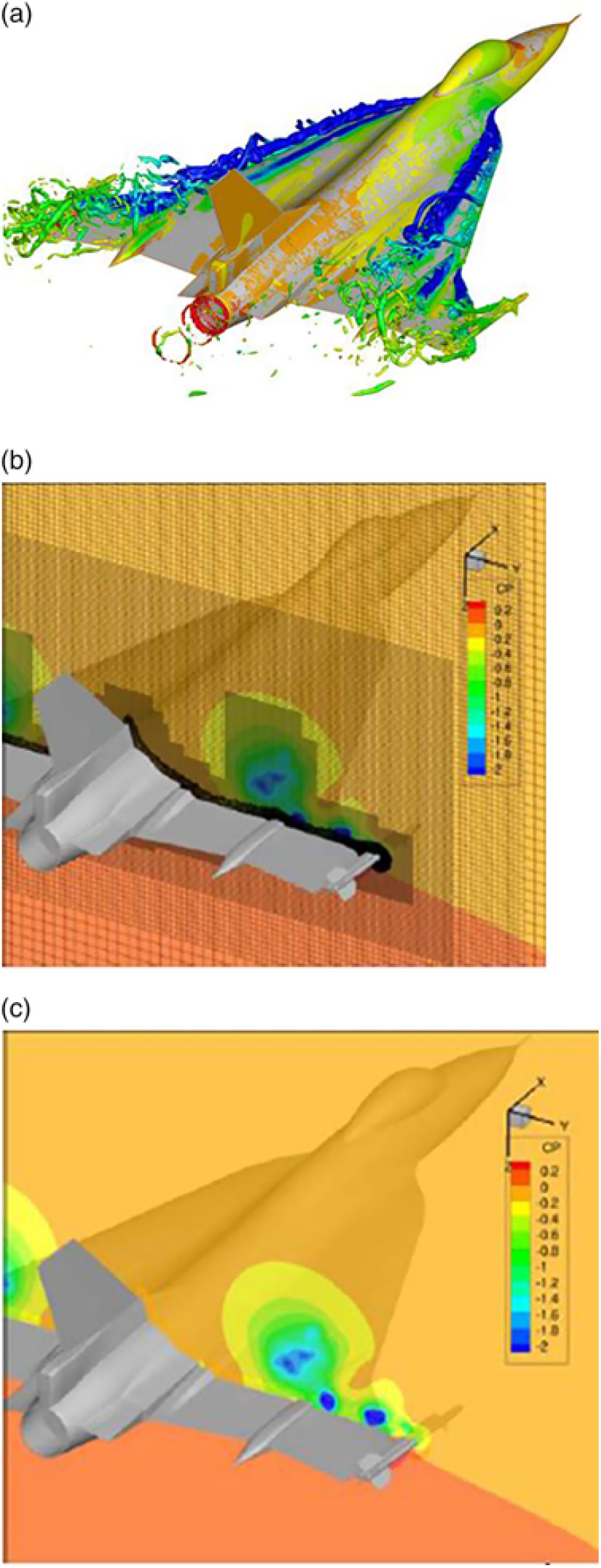
Figure 67. Adaptive mesh refinement solution, KESTREL. FC – 25: M = 0.24, Re cref = 32 × 106, α = 19.8°. Morton and McDaniel(Reference Morton and McDaniel132). (a) Flowfield. (b) Unsteady flow simulation, surface pressures. (a) Flowfield. (b) Near-body and off-body grids. (c) Vortex resolution.
Detailed unsteady vortex simulations were performed by all partners using hybrid RANS/LES techniques, and the adaptive grid technology was demonstrated to provide significantly improved resolution of the interacting vortical flows. An example is shown in Fig. 67 from Morton and McDaniel(Reference Morton and McDaniel132) using the KESTREL code(Reference Morton, McDaniel, Sears, Tillman and Tuckey119) with AMR. Grids were adapted in both space and time, and a very fine resolution of the wing vortex flowfield was achieved. The most challenging pressure distribution for this case was at Butt Line 153.5, which is on the wing outer panel, and predictions from a second KESTREL simulation are shown in Fig. 68 from Lofthouse and Cummings(Reference Lofthouse and Cummings133). This unsteady simulation also used adaptive grids. Static surface pressure distributions from the unsteady simulation are shown for (i) mean values (ii) maximum and minimum values and (iii) mean plus/minus one standard deviation. Flight test data are also shown, and these data were measured using steady-flow sensor technology. Earlier CAWAPI work had interpreted these pressures as if they were steady, but from the CFD simulation, it is clear that the flow is very unsteady on the outer panel at this condition. No unsteady pressure measurements were taken during the F-16XL flight-test program, and thus no data are available to quantitatively assess the CAWAPI-3 unsteady flow simulations. It does appear, however, that unsteady flow effects are important to the wing outer-panel aerodynamics at this condition with interacting vortex flows. A summary of the CAWAPI-3 findings was published in 2017 in a special section of the AIAA Journal of Aircraft with an introduction by Luckring(Reference Luckring134).
Significant progress was made over the span of the CAWAPI work. The progress was realised not only through better understanding of the interacting vortex flows, but also due to significantly better grid resolution as well as an advancement of CFD technology. A summary of some grid statistics over the CAWAPI programs is shown in Table 1. This work evolved from RANS simulations with a median of approximately one million fixed-grid cells to hybrid RANS/LES simulations with a median of approximately 90 m adaptive-grid cells. The work was executed on a representative but reduced complexity F-16XL geometry; many simplifications were applied to the airframe geometry to enable the CFD simulations. Full airframe modelling with associated flow feature resolution would require significantly larger grids than those used during the CAWAPI investigations.
Table 1 CAWAPI Grid statistics

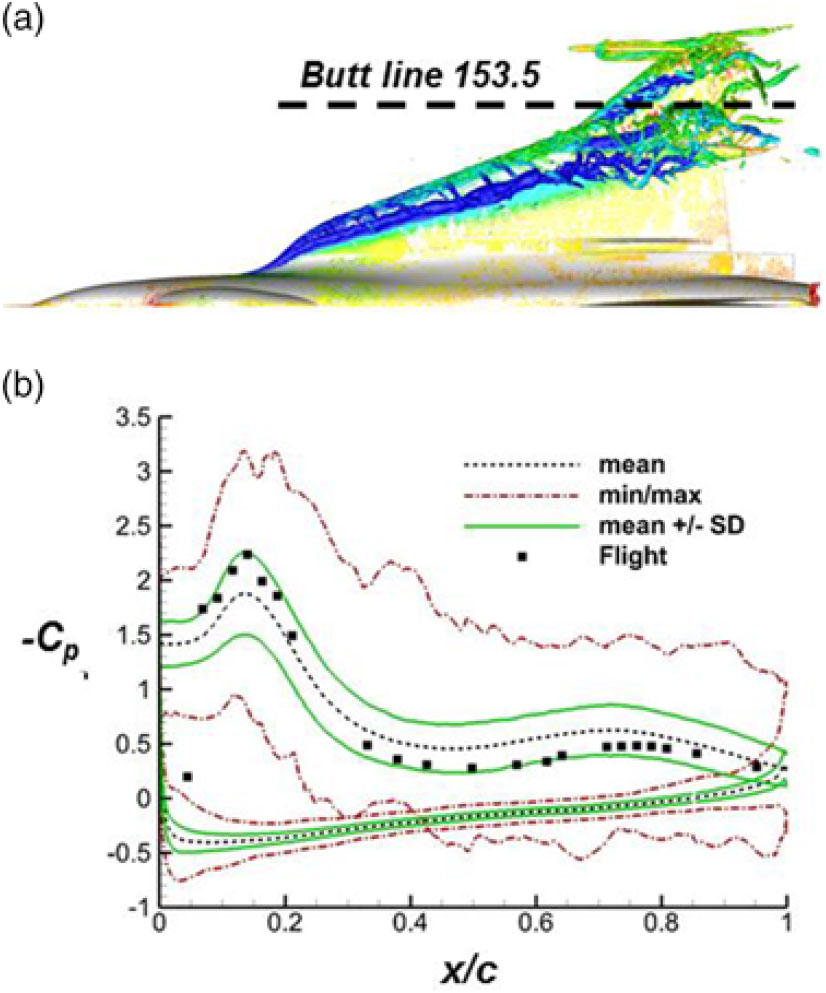
Figure 68. Outboard panel pressure analysis, KESTREL. FC – 25: M = 0.24, Re cref = 32 × 106, α = 19.8°. Lofthouse and Cummings(Reference Lofthouse and Cummings133).
The F-16XL data are very valuable, and yet it became clear that new experimentation would be needed to resolve the remaining vortex-interaction issues from the F-16XL research. Such tests could be designed from the perspective of CFD validation, and detailed measurements in carefully controlled wind-tunnel conditions would be needed to further guide improved simulation capability for these complex vortex interactions at both low-speed high angle-of-attack and high-speed low-angle-of-attack conditions. Some additional discussion of CFD validation testing is included in the next section.
6.0 CAPABILITY ASSESSMENT
The collective previous Section 5 summarised, from a historical perspective, the modelling for separation-induced vortex flows along with associated predictions of vortex flow aerodynamics. In this section, a summary capability assessment is presented from a more fundamental perspective of the vortex flow physics underlying the applications discussed. If the physics of some separation-induced vortex flow are correctly modelled and adequately resolved, then the consequences of the vortex for some configurational application (be it a delta wing or an aircraft) should be within grasp.
Proper flow physics modelling invokes validation principles which, by now, have been well established. (See, for example, references(135, Reference Oberkampf and Trucano136, 137, 138, Reference Oberkampf and Roy139)). Following the American Society of Mechanical Engineers (ASME) guide(137), validation can be defined as ‘the process of determining the degree to which a model is an accurate representation of the real world from the perspective of the intended uses of the model’. For contemporary CFD validation, it can be useful to consider the following questions:
1. Do we understand the critical flow physics underlying a particular flow phenomenon?
2. Do we understand how to numerically approximate these critical physics (e.g., turbulence models, grid resolution, temporal resolution)?
3. Do we have fundamental data to validate any such resultant numerical simulations?
4. Do we understand how these critical physics might be affected from ground to flight scales?
For virtually all current CFD validation interests, prior data sets are inadequate to answer these questions, and new experiments, designed from a validation perspective, are necessary. These experiments often involve detailed flowfield measurements within the flow phenomenon of interest (e.g., a secondary vortex) and can be challenging to accomplish. They also involve wind-tunnel boundary-condition measurements to facilitate the CFD validation simulations as well as test section flow characterisation and data uncertainty quantification to enable the CFD validation assessments. In this regard, validation testing constitutes a separate class of experimentation.
A summary status of validated CFD capability to predict the fundamental separation-induced vortex flows discussed in this article is presented in Table 2. All the vortex phenomena include unsteady effects but at different scales and to varying extents. For example, the primary vortex from sharp-edge slender wing at a moderate angle-of-attack can be very steady (unsteadiness occurs at small scales), whereas vortex breakdown exhibits unsteady flow at larger scales with greater effects.
Table 2 Vortex predictive capability

Capabilities were assessed from a validation perspective using the above questions, and except for the sharp-edge vortex from a slender wing, the capability is not very good. In most of these cases, validation data do not exist; even in the sharp-edge slender wing case, details for the vortical substructure that can occur within the primary vortex sheet (cf., Fig. 12) as well as details within the secondary vortex lack validation data sets. Transition flow physics can also affect secondary vortices and present another need for validation data sets.
Some fundamental knowledge of vortex breakdown has become well established for simplified cases, such as an isolated vortex in a circular tube (Liebovich(Reference Leibovich140), Grabowski and Berger(Reference Grabowski and Berger141)), but very little capability has been demonstrated for predicting the three-dimensional case, even for delta wings. Detailed validation measurements in the vortex core for 3D wings are needed but are very difficult to accomplish, not only due to intrusive technique sensitivities, but also due to an inherent departure of seeds from the vortex core velocity field for nonintrusive techniques (Greenwell(Reference Greenwell142)). Vortex breakdown is inherently an unsteady phenomenon that further complicates this validation challenge.
Regarding blunt-leading-edge vortices, a physical mechanism has been postulated by Hitzel et al.(Reference Hitzel, Boelens, Rooij and Hövelmann117) for the creation of the inner vortex. Validation data are needed to assess this concept in more detail as well as to validate simulations of the inner vortex at downstream stations. Incipient separation has been identified as the critical phenomenon for predicting the onset and progression of the blunt-leading-edge primary vortex separation. However, the incipient separation region occurs near and around the curved leading edge with very thin boundary layers and defies detailed measurement with contemporary techniques.
Given the validation challenges with an individual primary/secondary vortex system, the interactions amongst these vortical systems (a system of systems) remain a very challenging topic. For all of the interaction classes briefly identified in this paper (vortex-vortex, vortex-shock, and vortex-surface), our knowledge of these vortex interactions as well as our ability to predict these flows with contemporary CFD methods is inadequate and would greatly benefit from validation campaigns.
Unsteady effects for vortical flows merit additional discussion due to the added challenges of temporal resolution. Once again, fundamental knowledge has been established with work such as that due to Gursul, et al.(Reference Gursul, Gordnier and Visbal29) and Gordnier et al.(Reference Gordnier, Visbal, Gursul and Wang143). Unsteady vortical flows are exceptionally complex, difficult to compute and difficult to measure. Unsteady vortical simulations seem to require hybrid RANS/LES techniques, and carefully designed experimental campaigns are needed to generate time accurate data to validate these computationally intensive simulations.
It should be noted that the analysis reported herein has been for static rigid wings. Dynamic conditions introduce new unsteady effects to the vortical flows, including vortex hysteresis. Both static and dynamic aeroelasticity introduce additional challenges. New validation data sets will be needed to advance our knowledge and simulation capability for vortical effects associated with dynamic and aeroelastic conditions.
For all these vortex flow topics, it must also be recognised that grid resolution of the vortical flow structures has most likely been inadequate. The Stewartson and Hall(Reference Stewartson and Hall38) theoretical modelling demonstrated that boundary-layer-like length scales exist within the primary vortex, but these scales rarely, if ever, are grid resolved in contemporary or historical CFD assessments. Considering this, it appears likely that very many separation-induced vortex simulations within the literature database could have under-resolved vortex flow physics. Adaptive grid technology for time-dependent spatial resolution seems to be a necessary technology to improve grid resolution of the off-body vortical structures.
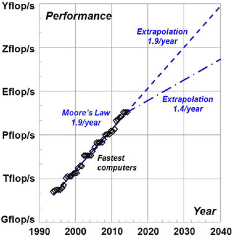
Figure 69. Computer performance.
Of course, grid resolution is always constrained by contemporary supercomputer capacity, regarding both memory and speed. Solutions need to be realised quickly enough to contribute to program interests, processing time is proportional to problem size and grid size constraints limit geometric representation and flowfield resolution. Moore’s law has been useful to estimate how much improvement in processing time can be anticipated from supercomputer evolution, as seen in Fig. 69. Current CFD simulations of complex configurations can use 500 m points without fully modelling the full scale vehicle of interest, and in one recent example(Reference Krist, Ratnayake and Ghaffari144) at NASA, approximately 4 Bn cells were needed to model a complex Space Launch System configuration with complex vortical flows. Full-scale configuration geometry had already been significantly simplified, roughly to that of a wind-tunnel model, and adaptive grids were used to help resolve the vortex flows with some efficiency. For this problem size, solutions took two to three weeks to accumulate eight to nine days of processing time in a shared-resource supercomputing environment. It is estimated(Reference Krist145) that roughly an order of magnitude increase in grids could be anticipated for representing full-scale geometry along with a doubling in the cycles required for convergence with this grid at full-scale Reynolds numbers. Processing speed would have to increase by a factor of 20 to solve this full-scale simulation using the same nine days of processing time (all other factors being held constant), and another factor of 400 would be needed to change the nine days to 30 minutes of processing time to enable same-day analysis capability in support of program needs. By Moore’s law, this combined factor of 8,000 will take approximately 14 years to realise through supercomputer evolution with a frozen level of physics simulation (in this example, hybrid RANS/LES). Improved vortex resolution for the viscous flow-physics scales, as discussed in Section 5.1.2 of this paper, would further increase the supercomputer requirements as would any advancements to the simulation equation set (e.g., Direct Numerical Simulation (DNS)). Moreover, Spalart and Venkatakrishnan(Reference Spalart and Venkatakrishnan146) point out that Moore’s law extrapolations may now overestimate future supercomputer performance due to fundamental chip limitations; anticipated growth may only be at roughly half the Moore’s law rate, with possibly even less speed increase realised for typical CFD applications. Conventional computer advancements alone will not be enough for CFD to contribute timely results of grid-resolved flows for full-scale vehicle simulations. There is a sustained need for advanced algorithm development, both in regards to speed as well as flow physics resolution (e.g., adaptive grids) and representation (e.g., transitional flows). Guidance from new experimentation could contribute to the new flow physics representations.
Despite the present validation deficiencies for the separation-induced vortex flows as well as the current supercomputer constraints on problem size (and, hence, resolution), many useful applications for configuration aerodynamics assessments have been accomplished for fairly complex configurations with complex vortical flows. These experiences, combined with the theoretical foundation established for vortex flows, could guide the development of targeted CFD validation campaigns for capability enhancements. These assessments, with anticipated CFD improvements, could help ameliorate many of the current limitations and, thereby, enhance the predictive capability for separation-induced leading-edge vortices and vortex flow aerodynamics.
7.0 CONCLUDING REMARKS
A review has been presented of separation-induced leading-edge vortex flows that pertain to wing aerodynamics. This has included the earliest discussion of these flows that came from experimentation as well as the evolution of theoretical modelling and numerical simulation of these flows for the prediction of configuration aerodynamics, a topic referred to as vortex flow aerodynamics. The paper has been written with a view towards the underlying physics of these vortical flows and included capability assessment for predicting the flows from this physics-based perspective.
The two experiments that appear to be at the origins of separation-induced vortex flows for wings raised awareness for both some physical aspects of the vortex flows and the consequences of the vortex flows for airframe aerodynamics. At the time of these experimental findings, there were no theoretical means for predicting these vortex flow effects. The subsequent theoretical modelling activities were heavily informed by on-going experimental research. Many of the experimental programs were motivated by configuration development interests with the benefit of aligning the method development research with national programs. Other experiments were motivated more towards understanding the underlying flow physics of the vortex flows, although even in these cases, the fundamental work was still relevant to contemporary vehicle development interests.
Today’s predictive capability is anchored in CFD methods that can capture vortex flows. Promising vortical simulations on complex configurations have been demonstrated, originally with RANS technology and more recently with hybrid RANS/LES methods. It appears as if the hybrid RANS/LES technology, with adaptive mesh refinement, will be required for many of the contemporary vortex flow simulation interests. These computations are taxing for current supercomputers, and supercomputer evolution alone will be inadequate to allow the simulation needed to address many current interests in a timely manner. The need for faster algorithms is still present.
The collective CFD simulation experience for separation-induced vortex flows on complex configurations has also identified a number of fundamental gaps in our knowledge of these flows. Other gaps have been found from integrated numerical/experimental campaigns of a more fundamental nature. For a number of these gaps there is sufficient knowledge to design new integrated numerical/experimental campaigns, from a validation perspective, to reduce, or possibly eliminate, these deficiencies. Other aerodynamic disciplines are gaining experience with this class of investigation that includes both advanced computation and complex wind-tunnel testing. Application of this approach could enhance our ability to simulate separation-induced vortex flows that are relevant to configuration aerodynamics.
Lovell(Reference Lovell147) presented the keynote address at an RTO symposium entitled ‘Vortex Flows and High Angle of Attack for Military Vehicles’ in 2001, and in this paper, he identified three domains of separation-induced vortex flows for configuration aerodynamics to which this author has added a fourth domain:
1. Those that are designed into the vehicle or component to improve system performance [exploit]
2. Those that are anticipated, but whose effects must be ameliorated [tolerate]
3. Those that were unforeseen or have unforeseen consequences [resolve]
4. Those that are designed out of the vehicle or component to improve system performance [avoid]
All these possibilities require reliable numerical and experimental simulation capability of the vortex flows, and the fourth domain has the added challenge of determining the onset of a flow state change from attached to separated vortical flow. Although developed with a focus on military vehicle aerodynamics, his logic applies to other vehicle classes across a spectrum of scales identified in this report for which vortex flow aerodynamics can be manifested. It is at least possible that new research programs targeted at fundamental knowledge gaps for vortex flows from one vehicle class perspective could contribute to vortex flow interests from other application domains.

Figure 70. Theoreticians, slender-wing and vortex flow aerodynamics. (a) Robert T. Jones, NACA Langley. (b) Robert Legendre, ONERA. (c) Clinton E. Brown, NACA Langley. (d) William H. Michael, Jr., NACA Langley. (e) Kurt W. Mangler, RAE. (f) Jeremy H. B. Smith, RAE. (g) M. G. Hall, RAE. (h) Keith Stewartson, RAE. (i) Susan N. Brown, University College London. (j) Johanna Weber, RAE. (k) Edward C. Polhamus, NASA Langley.
Acknowledgements
This author wishes to acknowledge the theoreticians who contributed to the original modelling of separation-induced leading-edge vortices and their effects on vortex flow aerodynamics, Fig. 70. Their pioneering research contributed valuable insights to the physics of these vortex flows as well as their effects on wing aerodynamics. The author greatly appreciates the opportunity provided at the NASA Langley Research Center for performing the research that led to this article. The author also wishes to thank Ms. Dorothy Notarnicola at the NASA Langley Technical Library for sustained literature research support. The author’s time was supported, in part, by the by the Transformative Aeronautics Concepts (TAC) Program and the Transformational Tools and Technologies (TTT) Project, and this support is greatly appreciated.

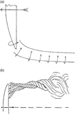

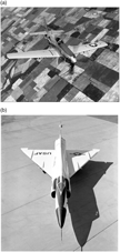

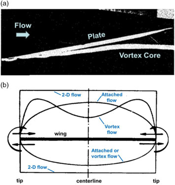

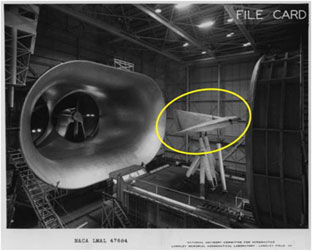

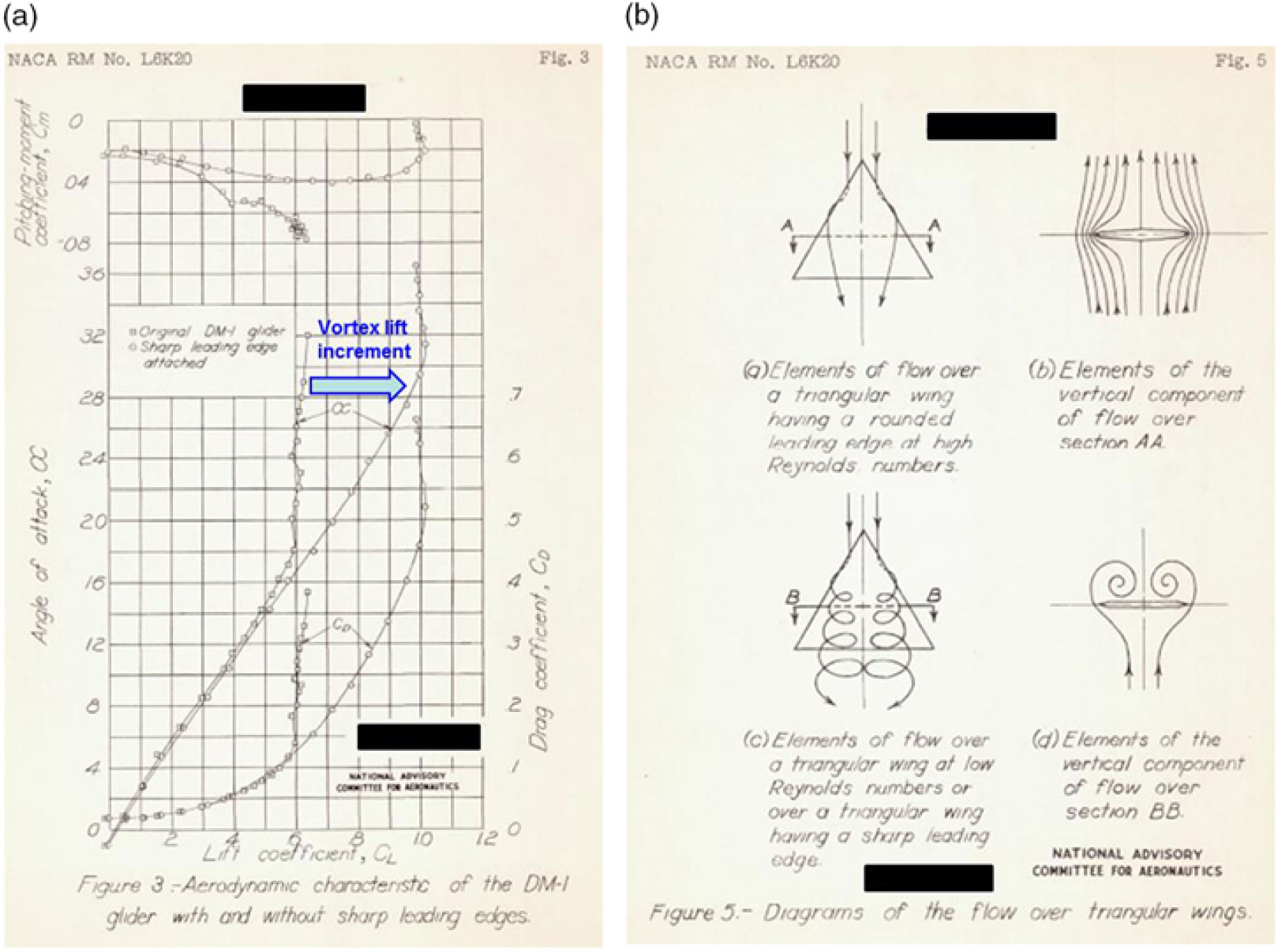
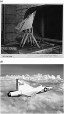

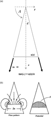


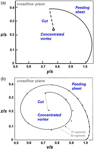

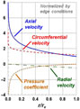
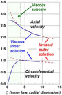

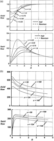


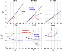


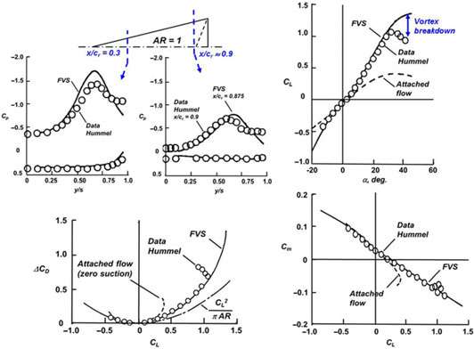

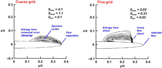

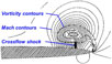

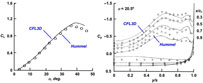


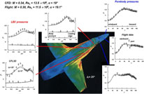


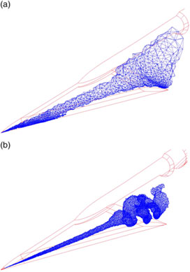


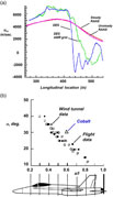

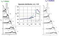

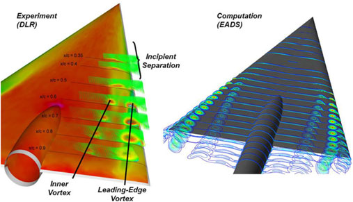
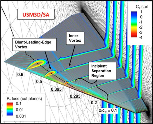
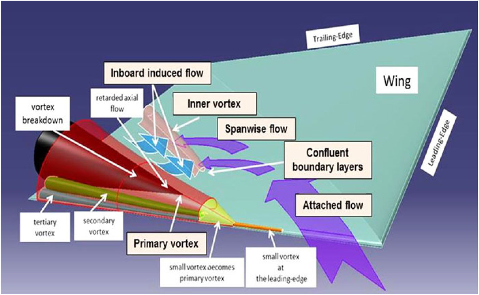
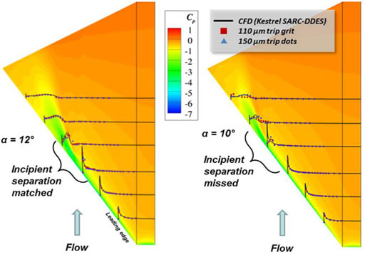

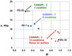

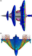


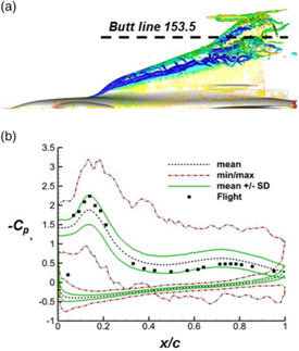
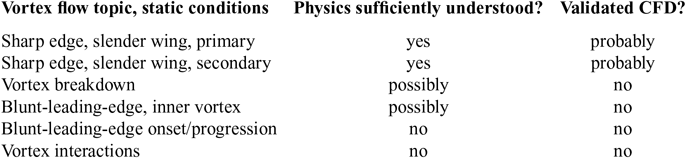


 Open access