


1 Introduction
Cylindrical structures are widely used in the marine offshore industry, for example, the hull of a spar platform (Saiful-Islam et al.
Reference Saiful-Islam, Jameel, Jumaat, Shirazi and Salman2012), deep-water risers (Carter & Ronalds Reference Carter and Ronalds1998), etc. Wake flow behind circular cylinders has been a popular topic of investigation for researchers and engineers for decades. It is well known that when the Reynolds number ( $Re_{D}$
) is less than 50, the wake flow around a circular cylinder is laminar and steady, and there is no vortex shedding behind the cylinder (Williamson Reference Williamson1996). For
$Re_{D}$
) is less than 50, the wake flow around a circular cylinder is laminar and steady, and there is no vortex shedding behind the cylinder (Williamson Reference Williamson1996). For $50\lesssim Re_{D}\lesssim 180$
, periodic two-dimensional vortex shedding occurs in the wake behind the cylinder. When
$50\lesssim Re_{D}\lesssim 180$
, periodic two-dimensional vortex shedding occurs in the wake behind the cylinder. When $Re_{D}$
exceeds 180, the wake becomes three-dimensional. The well-known mode A and mode B appear at
$Re_{D}$
exceeds 180, the wake becomes three-dimensional. The well-known mode A and mode B appear at $Re_{D}=180{-}194$
and
$Re_{D}=180{-}194$
and $Re_{D}=200{-}250$
, respectively (Williamson Reference Williamson1996). Wake turbulence and shear layer instabilities follow as
$Re_{D}=200{-}250$
, respectively (Williamson Reference Williamson1996). Wake turbulence and shear layer instabilities follow as $Re_{D}$
further increases.
$Re_{D}$
further increases.
However, even at $Re_{D}\lesssim 180$
, we can observe three-dimensional cylinder wakes under certain circumstances, such as cylinders with non-uniform inflow, cylinders with varying cross-sections, cylinders with free ends, etc. In these cases, three-dimensionality is triggered by spanwise non-uniformity in either the incoming flow or the configuration itself. Complex three-dimensional wake dynamics appear, such as vortex split, vortex dislocation and oblique shedding. In order to investigate these complex flow phenomena, a single step cylinder becomes an ideal configuration in which geometric complications are removed except for the sudden diameter change.
$Re_{D}\lesssim 180$
, we can observe three-dimensional cylinder wakes under certain circumstances, such as cylinders with non-uniform inflow, cylinders with varying cross-sections, cylinders with free ends, etc. In these cases, three-dimensionality is triggered by spanwise non-uniformity in either the incoming flow or the configuration itself. Complex three-dimensional wake dynamics appear, such as vortex split, vortex dislocation and oblique shedding. In order to investigate these complex flow phenomena, a single step cylinder becomes an ideal configuration in which geometric complications are removed except for the sudden diameter change.
1.1 Single step cylinder wake
There are two important parameters in the wake flow behind a single step cylinder, i.e. the Reynolds number ( $Re_{D}$
) and the diameter ratio (
$Re_{D}$
) and the diameter ratio ( $D/d$
). The latter,
$D/d$
). The latter, $D/d$
, is the ratio between the large- and small-diameter parts of the step cylinder, while
$D/d$
, is the ratio between the large- and small-diameter parts of the step cylinder, while $Re_{D}=UD/\unicode[STIX]{x1D708}$
(where
$Re_{D}=UD/\unicode[STIX]{x1D708}$
(where $U$
represents the uniform inflow velocity, and
$U$
represents the uniform inflow velocity, and $\unicode[STIX]{x1D708}$
is the kinematic viscosity of the fluid).
$\unicode[STIX]{x1D708}$
is the kinematic viscosity of the fluid).
The wake of step cylinders with $1.14<D/d<1.76$
at
$1.14<D/d<1.76$
at $67<Re_{D}<200$
was initially investigated by Lewis & Gharib (Reference Lewis and Gharib1992). They reported two vortex interaction modes: a direct and an indirect mode. The direct mode occurs when
$67<Re_{D}<200$
was initially investigated by Lewis & Gharib (Reference Lewis and Gharib1992). They reported two vortex interaction modes: a direct and an indirect mode. The direct mode occurs when $D/d<1.25$
, where two dominating shedding frequencies (
$D/d<1.25$
, where two dominating shedding frequencies ( $f_{S}$
and
$f_{S}$
and $f_{L}$
) correspond to vortices shed from the small and large cylinders, respectively. The interactions between these two kinds of vortices take place in a narrow region referred to as the interface. When they are in phase, vortices from the two wake regions connect to each other one by one across the interface. When they are out of phase, the direct connection will be interrupted and at least one half-loop connection between oppositely rotating vortices will appear. The period between two such interruptions is called a beat cycle. In the indirect mode (
$f_{L}$
) correspond to vortices shed from the small and large cylinders, respectively. The interactions between these two kinds of vortices take place in a narrow region referred to as the interface. When they are in phase, vortices from the two wake regions connect to each other one by one across the interface. When they are out of phase, the direct connection will be interrupted and at least one half-loop connection between oppositely rotating vortices will appear. The period between two such interruptions is called a beat cycle. In the indirect mode ( $D/d>1.55$
), in addition to
$D/d>1.55$
), in addition to $f_{S}$
and
$f_{S}$
and $f_{L}$
, another distinct frequency
$f_{L}$
, another distinct frequency $f_{3}$
(which is referred to as
$f_{3}$
(which is referred to as $f_{N}$
in the present paper) can be detected near the interface behind the large cylinder. This region was first named the modulation zone by Lewis & Gharib (Reference Lewis and Gharib1992). It prevents direct interactions between the vortices with shedding frequency
$f_{N}$
in the present paper) can be detected near the interface behind the large cylinder. This region was first named the modulation zone by Lewis & Gharib (Reference Lewis and Gharib1992). It prevents direct interactions between the vortices with shedding frequency $f_{S}$
and those with shedding frequency
$f_{S}$
and those with shedding frequency $f_{L}$
. In the modulation zone, the velocity variation is modulated by the main frequency behind the large cylinder, and an inclined interface was found to occur at a beat frequency
$f_{L}$
. In the modulation zone, the velocity variation is modulated by the main frequency behind the large cylinder, and an inclined interface was found to occur at a beat frequency $(f_{L}-f_{N})$
. Lewis & Gharib (Reference Lewis and Gharib1992) found that the vortex interactions in the indirect mode are more complex than in the directmode.
$(f_{L}-f_{N})$
. Lewis & Gharib (Reference Lewis and Gharib1992) found that the vortex interactions in the indirect mode are more complex than in the directmode.
Based on the three dominating shedding frequencies, Dunn & Tavoularis (Reference Dunn and Tavoularis2006) identified three types of spanwise vortices: (1) S-cell vortex shed from the small cylinder with the highest shedding frequency $f_{S}$
, (2) N-cell vortex shed in the modulation zone with the lowest shedding frequency
$f_{S}$
, (2) N-cell vortex shed in the modulation zone with the lowest shedding frequency $f_{N}$
, and (3) L-cell vortex shed from the large cylinder with shedding frequency
$f_{N}$
, and (3) L-cell vortex shed from the large cylinder with shedding frequency $f_{L}$
. The terminologies S-, N- and L-cell were thereafter adopted in many studies (Morton, Yarusevych & Carvajal-Mariscal Reference Morton, Yarusevych and Carvajal-Mariscal2009; Morton & Yarusevych Reference Morton and Yarusevych2010a
,Reference Morton and Yarusevych
b
, Reference Morton and Yarusevych2014; Tian et al.
Reference Tian, Jiang, Pettersen and Andersson2017a
,Reference Tian, Jiang, Pettersen and Andersson
b
), and are also used in the present study. The regions where these vortex cells occur are indicated in figure 1(a).
$f_{L}$
. The terminologies S-, N- and L-cell were thereafter adopted in many studies (Morton, Yarusevych & Carvajal-Mariscal Reference Morton, Yarusevych and Carvajal-Mariscal2009; Morton & Yarusevych Reference Morton and Yarusevych2010a
,Reference Morton and Yarusevych
b
, Reference Morton and Yarusevych2014; Tian et al.
Reference Tian, Jiang, Pettersen and Andersson2017a
,Reference Tian, Jiang, Pettersen and Andersson
b
), and are also used in the present study. The regions where these vortex cells occur are indicated in figure 1(a).

Figure 1. Vortex shedding in the wake behind a step cylinder. (a) Isosurfaces of $\unicode[STIX]{x1D706}_{2}=-0.05$
(Jeong & Hussain Reference Jeong and Hussain1995) from our simulation, at
$\unicode[STIX]{x1D706}_{2}=-0.05$
(Jeong & Hussain Reference Jeong and Hussain1995) from our simulation, at $Re_{D}=150$
and
$Re_{D}=150$
and $D/d=2$
. (b) Isosurfaces of
$D/d=2$
. (b) Isosurfaces of $Q\approx 2\times 10^{-3}$
from Morton & Yarusevych (Reference Morton and Yarusevych2010b
), at
$Q\approx 2\times 10^{-3}$
from Morton & Yarusevych (Reference Morton and Yarusevych2010b
), at $Re_{D}=150$
and
$Re_{D}=150$
and $D/d=2$
(image reproduced from Morton & Yarusevych (Reference Morton and Yarusevych2010b
), with the permission of AIP Publishing). (c) Flow visualization image from Dunn & Tavoularis (Reference Dunn and Tavoularis2006), at
$D/d=2$
(image reproduced from Morton & Yarusevych (Reference Morton and Yarusevych2010b
), with the permission of AIP Publishing). (c) Flow visualization image from Dunn & Tavoularis (Reference Dunn and Tavoularis2006), at $Re_{D}=150$
and
$Re_{D}=150$
and $D/d=1.98$
(image reproduced from Dunn & Tavoularis (Reference Dunn and Tavoularis2006) with permission from Cambridge University Press).
$D/d=1.98$
(image reproduced from Dunn & Tavoularis (Reference Dunn and Tavoularis2006) with permission from Cambridge University Press).
The interactions between different vortex cells in the indirect mode were investigated in the wake behind a single step cylinder with $D/d\approx 2$
and
$D/d\approx 2$
and $Re_{D}\approx 150$
, experimentally by Dunn & Tavoularis (Reference Dunn and Tavoularis2006) and numerically by Morton & Yarusevych (Reference Morton and Yarusevych2010b
). These studies concluded that the S–N cell boundary (the region between the S- and N-cell vortices) is stable and deflects spanwise into the large cylinder direction. At this boundary, one N-cell vortex always connects to a counter-rotating N-cell mate and an S-cell vortex. The vortex dislocations between the S- and N-cell vortices occur at a beat frequency (
$Re_{D}\approx 150$
, experimentally by Dunn & Tavoularis (Reference Dunn and Tavoularis2006) and numerically by Morton & Yarusevych (Reference Morton and Yarusevych2010b
). These studies concluded that the S–N cell boundary (the region between the S- and N-cell vortices) is stable and deflects spanwise into the large cylinder direction. At this boundary, one N-cell vortex always connects to a counter-rotating N-cell mate and an S-cell vortex. The vortex dislocations between the S- and N-cell vortices occur at a beat frequency ( $f_{S}-f_{N}$
) at the S–N cell boundary. During this dislocation process, the half-loop connection between S-cell vortices is dominating. The number of S- and N-cell vortices in a cyclic period (from one dislocation process to the next) is determined by the ratio of the shedding frequencies of these two cells (
$f_{S}-f_{N}$
) at the S–N cell boundary. During this dislocation process, the half-loop connection between S-cell vortices is dominating. The number of S- and N-cell vortices in a cyclic period (from one dislocation process to the next) is determined by the ratio of the shedding frequencies of these two cells ( $f_{S}/f_{N}$
).
$f_{S}/f_{N}$
).
Unlike the S–N cell boundary, the N–L cell boundary (the region between the N- and L-cell vortices) is unstable. As the phase difference between the N- and L-cell vortices accumulates, in parallel with the appearance of vortex dislocations between N- and L-cell vortices, the shapes and lengths of the N-cell vortices and the position of the N–L cell boundary vary periodically with the beat frequency ( $f_{L}-f_{N}$
). Morton & Yarusevych (Reference Morton and Yarusevych2010b
) defined these cyclic changes as the N-cell cycle. Tian et al. (Reference Tian, Jiang, Pettersen and Andersson2017a
) further investigated the dislocation processes at the N–L cell boundary. Two new loop structures were identified: the NL-loop (the fake loop) formed between a pair of N- and L-cell vortices with opposite rotating directions, and the NN-loop (the real loop) formed between two subsequent N-cell vortices with opposite rotating directions. In addition, antisymmetric vortex interactions between two adjacent N-cell cycles were reported based on careful observations of the development of these two kinds of loop structures.
$f_{L}-f_{N}$
). Morton & Yarusevych (Reference Morton and Yarusevych2010b
) defined these cyclic changes as the N-cell cycle. Tian et al. (Reference Tian, Jiang, Pettersen and Andersson2017a
) further investigated the dislocation processes at the N–L cell boundary. Two new loop structures were identified: the NL-loop (the fake loop) formed between a pair of N- and L-cell vortices with opposite rotating directions, and the NN-loop (the real loop) formed between two subsequent N-cell vortices with opposite rotating directions. In addition, antisymmetric vortex interactions between two adjacent N-cell cycles were reported based on careful observations of the development of these two kinds of loop structures.
When $Re_{D}$
increases, the wake gradually becomes more complex. However, the three dominating spanwise vortices (S-, N- and L-cell vortices), the vortex dislocation between them and the cyclic variation of the N-cell vortices are still observable in the wake flow (Morton & Yarusevych Reference Morton and Yarusevych2010b
). In addition, Morton & Yarusevych (Reference Morton and Yarusevych2010a
, Reference Morton and Yarusevych2014) reported that the duration of the N-cell cycle varies and fits a Gaussian distribution at relatively high
$Re_{D}$
increases, the wake gradually becomes more complex. However, the three dominating spanwise vortices (S-, N- and L-cell vortices), the vortex dislocation between them and the cyclic variation of the N-cell vortices are still observable in the wake flow (Morton & Yarusevych Reference Morton and Yarusevych2010b
). In addition, Morton & Yarusevych (Reference Morton and Yarusevych2010a
, Reference Morton and Yarusevych2014) reported that the duration of the N-cell cycle varies and fits a Gaussian distribution at relatively high $Re_{D}=1050$
.
$Re_{D}=1050$
.
Other characteristics of the wake behind a single step cylinder with different diameter ratios and different Reynolds numbers have been discussed in several papers. Ko, Leung & Au (Reference Ko, Leung and Au1982), Yagita, Yoshihiro & Matsuzaki (Reference Yagita, Yoshihiro and Matsuzaki1984), Norberg (Reference Norberg1992) and Dunn & Tavoularis (Reference Dunn and Tavoularis2006) found that the vortex shedding behind the small cylinder was seldom influenced, but the flow behind the large cylinder was strongly affected by the step. When this induced effect becomes strong enough, N-cell vortices appear (Norberg Reference Norberg1992; Dunn & Tavoularis Reference Dunn and Tavoularis2006). In addition to the three main vortex cells (S, N and L), two pairs of streamwise vortices (i.e. junction vortices and edge vortices) have also been identified around the step region (Dunn & Tavoularis Reference Dunn and Tavoularis2006; Morton et al. Reference Morton, Yarusevych and Carvajal-Mariscal2009; Tian et al. Reference Tian, Jiang, Pettersen and Andersson2017b ).
1.2 Vortex dislocation
It is widely accepted that most of the observations mentioned above for the step cylinder are closely related to vortex dislocations. As an interesting physical phenomenon, vortex dislocations have also been investigated in various types of flow, such as in uniform cylinder wakes, mixing layers and nonlinear waves.
The phrase vortex dislocation was first introduced by Williamson (Reference Williamson1989) when he observed multiple vortex cells with different shedding frequencies in his experiments of flow past a circular cylinder at $Re_{D}<200$
. Neighbouring vortex cells are observed to move either in phase or out of phase with each other due to their different shedding frequencies. When these vortex cells move out of phase, at the boundary between them, the contorted ‘tangle’ of vortices appears and looks like dislocations that appear in solid materials. Williamson (Reference Williamson1989) defined this kind of flow phenomenon as vortex dislocation. He reported that, at
$Re_{D}<200$
. Neighbouring vortex cells are observed to move either in phase or out of phase with each other due to their different shedding frequencies. When these vortex cells move out of phase, at the boundary between them, the contorted ‘tangle’ of vortices appears and looks like dislocations that appear in solid materials. Williamson (Reference Williamson1989) defined this kind of flow phenomenon as vortex dislocation. He reported that, at $Re_{D}=100$
, vortex dislocations occur at the boundary between cells (the end-plate cell of frequency
$Re_{D}=100$
, vortex dislocations occur at the boundary between cells (the end-plate cell of frequency $f_{e}$
and the single cell of frequency
$f_{e}$
and the single cell of frequency $f_{L}$
) at a constant beat frequency
$f_{L}$
) at a constant beat frequency $f_{L}-f_{e}$
, accompanied by an obvious minimum amplitude of the velocity fluctuations at the boundary. In addition, by comparing velocity signals from different vortex cell regions, the time trace of phase differences was plotted. Williamson (Reference Williamson1992) further investigated the dislocation by adding a small ‘ring’ on a circular cylinder in order to force the dislocation to happen. This study revealed more detailed features of vortex dislocations, such as the vortex dynamics and the effects of vortex dislocations in the wake flow. An interesting long-period characteristic of the vortex dislocation was first reported in McClure, Morton & Yarusevych (Reference McClure, Morton and Yarusevych2015) by investigating flow past dual step cylinders. They defined the time period between two identical vortex dislocations as the fundamental dislocation cycle. Further investigations of this characteristic in the wake behind the single step cylinder can be found in Tian et al. (Reference Tian, Jiang, Pettersen and Andersson2019). Vortex dislocations in other types of wakes and mixing layers have been reported by many others. For details, the reader is referred to the works of Gaster (Reference Gaster1969), Eisenlohr & Eckelmann (Reference Eisenlohr and Eckelmann1989) and Dallard & Browand (Reference Dallard and Browand1993).
$f_{L}-f_{e}$
, accompanied by an obvious minimum amplitude of the velocity fluctuations at the boundary. In addition, by comparing velocity signals from different vortex cell regions, the time trace of phase differences was plotted. Williamson (Reference Williamson1992) further investigated the dislocation by adding a small ‘ring’ on a circular cylinder in order to force the dislocation to happen. This study revealed more detailed features of vortex dislocations, such as the vortex dynamics and the effects of vortex dislocations in the wake flow. An interesting long-period characteristic of the vortex dislocation was first reported in McClure, Morton & Yarusevych (Reference McClure, Morton and Yarusevych2015) by investigating flow past dual step cylinders. They defined the time period between two identical vortex dislocations as the fundamental dislocation cycle. Further investigations of this characteristic in the wake behind the single step cylinder can be found in Tian et al. (Reference Tian, Jiang, Pettersen and Andersson2019). Vortex dislocations in other types of wakes and mixing layers have been reported by many others. For details, the reader is referred to the works of Gaster (Reference Gaster1969), Eisenlohr & Eckelmann (Reference Eisenlohr and Eckelmann1989) and Dallard & Browand (Reference Dallard and Browand1993).
1.3 Objectives of the present study
There have been many attempts to describe the vortex dislocations in the step cylinder wake. Previous studies pointed out that it is the accumulation of phase differences that causes the vortex dislocation between different adjacent spanwise vortex cells. However, the investigations of how phase differences accumulate and how they affect the vortex dislocations are still limited.
Williamson (Reference Williamson1989) and Lewis & Gharib (Reference Lewis and Gharib1992) experimentally examined the time trace of the phase difference by using probes to monitor velocity signals in different vortex cell regions positioned 10 cylinder diameters downstream. However, at such a location, oblique vortex shedding, complex vortex interactions and the stretching and tilting of the vortices make it difficult to accurately evaluate phase differences. Another interesting phenomenon in the wake flow behind the step cylinder is the cyclic changes of the N-cell vortex, which was defined as the N-cell cycle by Morton & Yarusevych (Reference Morton and Yarusevych2010b ). However, they analysed this phenomenon in a relatively short time period containing only a few N-cell cycles. Whether N-cell cycles have any long-period variations or very low-frequency features is still unknown.
The primary goal of the present numerical study is to thoroughly investigate the mechanisms of phase difference accumulation in the step cylinder wake, and their effect on vortex interactions. Considering that the wake behind the small cylinder part is seldom influenced by the step, and the contributions of the streamwise vortices on the vortex dislocation between the S- and N-cell vortices are unclear, we only focus on the vortex dislocation between the N- and L-cell vortices. To achieve this objective, we analyse the time and space signals of several flow quantities (velocity, vorticity and $\unicode[STIX]{x1D706}_{2}$
) obtained from a direct numerical simulation (DNS) of flow past two different step cylinders with diameter ratios
$\unicode[STIX]{x1D706}_{2}$
) obtained from a direct numerical simulation (DNS) of flow past two different step cylinders with diameter ratios $D/d=2$
and 2.4. In order to change the diameter ratio of the step cylinder, we keep
$D/d=2$
and 2.4. In order to change the diameter ratio of the step cylinder, we keep $D$
constant, and change
$D$
constant, and change $d$
. These two cases share the same coordinate system, computational method and data analysis process.
$d$
. These two cases share the same coordinate system, computational method and data analysis process.
First, in §§ 2–5, the flow problem, the numerical settings and analyses of the wake flow field are described in detail based on the $D/d=2$
case. Then, in § 6, the universality of our discussions and conclusions is studied by investigating the
$D/d=2$
case. Then, in § 6, the universality of our discussions and conclusions is studied by investigating the $D/d=2.4$
case. Last but not least, we also aim to present a reliable method that can be used to calculate the phase information (
$D/d=2.4$
case. Last but not least, we also aim to present a reliable method that can be used to calculate the phase information ( $\unicode[STIX]{x1D711}$
) and phase difference (
$\unicode[STIX]{x1D711}$
) and phase difference ( $\unicode[STIX]{x1D6F7}$
) of vortices, since such a method is lacking in the literature. Details of the method are included in appendix A.
$\unicode[STIX]{x1D6F7}$
) of vortices, since such a method is lacking in the literature. Details of the method are included in appendix A.
2 Flow configuration and computational aspects
2.1 Flow configuration and coordinate system
A sketch of the $D/d=2$
step cylinder geometry is shown in figure 2(a), where
$D/d=2$
step cylinder geometry is shown in figure 2(a), where $L$
and
$L$
and $l$
represent the lengths of the large and small parts of the cylinder, respectively. In figure 2(b), the computational domain and coordinate system are shown, where
$l$
represent the lengths of the large and small parts of the cylinder, respectively. In figure 2(b), the computational domain and coordinate system are shown, where $x$
-,
$x$
-, $y$
- and
$y$
- and $z$
-directions correspond to the streamwise, cross-flow and spanwise directions, respectively. The origin is located in the centre of the interface between the small and large cylinders. The inlet plane is
$z$
-directions correspond to the streamwise, cross-flow and spanwise directions, respectively. The origin is located in the centre of the interface between the small and large cylinders. The inlet plane is $10D$
upstream from the centre of the step cylinder, while the outlet plane is
$10D$
upstream from the centre of the step cylinder, while the outlet plane is $20D$
downstream. The spanwise height of the domain is
$20D$
downstream. The spanwise height of the domain is $45D$
, of which the small and large cylinders occupy
$45D$
, of which the small and large cylinders occupy $15D$
$15D$ $(l)$
and
$(l)$
and $30D$
$30D$ $(L)$
, respectively. The width of the domain is
$(L)$
, respectively. The width of the domain is $20D$
. This domain is larger than that used by Morton & Yarusevych (Reference Morton and Yarusevych2010b
) for the same
$20D$
. This domain is larger than that used by Morton & Yarusevych (Reference Morton and Yarusevych2010b
) for the same $D/d$
and
$D/d$
and $Re_{D}$
. Boundary conditions applied in the present study are as follows.
$Re_{D}$
. Boundary conditions applied in the present study are as follows.

Figure 2. (a) A sketch of the step cylinder geometry ( $D/d=2$
). (b) Computational domain, origin and coordinate system illustrated from two different viewpoints. The diameter of the large cylinder,
$D/d=2$
). (b) Computational domain, origin and coordinate system illustrated from two different viewpoints. The diameter of the large cylinder, $D$
, is the length unit. The origin is located in the centre of the step, i.e. the interface between the small and large cylinders.
$D$
, is the length unit. The origin is located in the centre of the step, i.e. the interface between the small and large cylinders.
-
(i) The inlet boundary: uniform velocity profile, $u=U$
,
$v=0$
,
$w=0$
.
$u=U$
,
$v=0$
,
$w=0$
. -
(ii) The outlet boundary: Neumann boundary condition for velocity components (
$\unicode[STIX]{x2202}u/\unicode[STIX]{x2202}x=\unicode[STIX]{x2202}v/\unicode[STIX]{x2202}x=\unicode[STIX]{x2202}w/\unicode[STIX]{x2202}x=0$
) and constant zero pressure condition. -
(iii) The other four sides of the computational domain: free-slip boundary conditions (for the two vertical sides,
$v=0$
,
$\unicode[STIX]{x2202}u/\unicode[STIX]{x2202}y=\unicode[STIX]{x2202}w/\unicode[STIX]{x2202}y=0$
; for the two horizontal sides,
$w=0$
,
$\unicode[STIX]{x2202}u/\unicode[STIX]{x2202}z=\unicode[STIX]{x2202}v/\unicode[STIX]{x2202}z=0$
). -
(iv) The step cylinder surfaces: no slip and impermeable wall.


2.2 Computational method
For all cases in the present investigation, a thoroughly validated finite-volume-based numerical code MGLET (Manhart Reference Manhart2004) is used to directly solve the incompressible Navier–Stokes equations. The midpoint rule is used to approximate the surface integral of flow variables over the faces of the discrete volumes, leading to second-order accuracy in space. A third-order explicit low-storage Runge-Kutta scheme (Williamson Reference Williamson1980) is used for time integration with a constant time step $\unicode[STIX]{x0394}t$
that ensures a Courant–Friedrichs–Lewy (CFL) number smaller than 0.65. The pressure–velocity coupling is handled by solving a Poisson equation with Stone’s strongly implicit procedure (SIP) (Stone Reference Stone1968). The same code has recently also been used to investigate other complex flows, such as the spheroid wake (Jiang et al.
Reference Jiang, Andersson, Gallardo and Okulov2016) and the curved cylinder wake (Jiang, Pettersen & Andersson Reference Jiang, Pettersen and Andersson2019).
$\unicode[STIX]{x0394}t$
that ensures a Courant–Friedrichs–Lewy (CFL) number smaller than 0.65. The pressure–velocity coupling is handled by solving a Poisson equation with Stone’s strongly implicit procedure (SIP) (Stone Reference Stone1968). The same code has recently also been used to investigate other complex flows, such as the spheroid wake (Jiang et al.
Reference Jiang, Andersson, Gallardo and Okulov2016) and the curved cylinder wake (Jiang, Pettersen & Andersson Reference Jiang, Pettersen and Andersson2019).
All simulations are conducted on a staggered Cartesian mesh, while the solid surface of the step cylinder is handled by an immersed boundary method (IBM) (Peller et al.
Reference Peller, Duc, Tremblay and Manhart2006). The computational domain is divided into cubic Cartesian grid boxes, named level-1 boxes. In each of them, $N\times N\times N$
cubic Cartesian grid cells are uniformly distributed. In order to refine the grid regions in which complex flow phenomena take place, such as the regions close to the step cylinder geometry, the region around the ‘step’, the regions where vortex dislocations happen, etc., all the grid boxes (the level-1 boxes) are equally split into eight smaller cubic boxes (the level-2 boxes). In each level-2 box, there are also
$N\times N\times N$
cubic Cartesian grid cells are uniformly distributed. In order to refine the grid regions in which complex flow phenomena take place, such as the regions close to the step cylinder geometry, the region around the ‘step’, the regions where vortex dislocations happen, etc., all the grid boxes (the level-1 boxes) are equally split into eight smaller cubic boxes (the level-2 boxes). In each level-2 box, there are also $N\times N\times N$
cubic grid cells. Hence, the grid resolution on level 2 is two times finer than that on level 1. This splitting process goes on automatically until the finest grid level is reached. The overall properties of the grids for all simulations can be found in table 1. A schematic illustration of the mesh design is shown in figure 3.
$N\times N\times N$
cubic grid cells. Hence, the grid resolution on level 2 is two times finer than that on level 1. This splitting process goes on automatically until the finest grid level is reached. The overall properties of the grids for all simulations can be found in table 1. A schematic illustration of the mesh design is shown in figure 3.

Figure 3. An illustration of the multi-level grids: (a) a slice of the computational domain in the $x{-}z$
plane at
$x{-}z$
plane at $y/D=0$
, and (b) a slice of the computational domain in the
$y/D=0$
, and (b) a slice of the computational domain in the $x{-}y$
plane at
$x{-}y$
plane at $z/D=0^{-}$
(at the large diameter
$z/D=0^{-}$
(at the large diameter $D$
region). Each square represents the slice of a corresponding cubic Cartesian grid box that contains
$D$
region). Each square represents the slice of a corresponding cubic Cartesian grid box that contains $N\times N\times N$
grid cells. Here, there are five levels of grid boxes, where the first four levels are indicated by numbers. Owing to different minimum grid sizes, different cases have either five or six levels of grid boxes. (c) A zoom-in plot of the grid cells in the step region (red rectangle in panel (b)) for case 2.
$N\times N\times N$
grid cells. Here, there are five levels of grid boxes, where the first four levels are indicated by numbers. Owing to different minimum grid sizes, different cases have either five or six levels of grid boxes. (c) A zoom-in plot of the grid cells in the step region (red rectangle in panel (b)) for case 2.
Table 1. Detailed mesh information of all $D/d=2$
cases. The Reynolds number for all cases is
$D/d=2$
cases. The Reynolds number for all cases is $Re_{D}=UD/\unicode[STIX]{x1D708}=150$
.
$Re_{D}=UD/\unicode[STIX]{x1D708}=150$
.

2.3 Grid convergence study
Table 2 shows the Strouhal number ( $St$
) of the three dominating vortex cells (
$St$
) of the three dominating vortex cells ( $St_{S}=f_{S}D/U$
,
$St_{S}=f_{S}D/U$
, $St_{N}=f_{N}D/U$
and
$St_{N}=f_{N}D/U$
and $St_{L}=f_{L}D/U$
) behind the step cylinder calculated by a fast Fourier transform (FFT) of the time series of the streamwise velocity
$St_{L}=f_{L}D/U$
) behind the step cylinder calculated by a fast Fourier transform (FFT) of the time series of the streamwise velocity $u$
along a vertical sampling line positioned at
$u$
along a vertical sampling line positioned at $(x/D,y/D)=(0.6,0.2)$
. For these four cases, the differences between
$(x/D,y/D)=(0.6,0.2)$
. For these four cases, the differences between $St$
numbers of the same vortex cell are small. In figure 4(a), the distributions of mean streamwise velocity along the line AB (as indicated in inset figure 4(
$St$
numbers of the same vortex cell are small. In figure 4(a), the distributions of mean streamwise velocity along the line AB (as indicated in inset figure 4( $a_{1}$
)) for all four cases are plotted to illustrate the flow variation on the ‘step’ just in front of the small cylinder. The curves in figure 4(a) and a zoom-in view in the inset figure 4(
$a_{1}$
)) for all four cases are plotted to illustrate the flow variation on the ‘step’ just in front of the small cylinder. The curves in figure 4(a) and a zoom-in view in the inset figure 4( $a_{2}$
) clearly show a convergent tendency from case 1 to case 4, and there are only minor differences between case 3 and case 4. Moreover, figure 4(b) shows time traces of the spanwise velocity (
$a_{2}$
) clearly show a convergent tendency from case 1 to case 4, and there are only minor differences between case 3 and case 4. Moreover, figure 4(b) shows time traces of the spanwise velocity ( $w$
) in the N-cell formation region where the velocity varies dramatically with time. The fluctuations and the mean values of
$w$
) in the N-cell formation region where the velocity varies dramatically with time. The fluctuations and the mean values of $w$
from case 3 and case 4 almost coincide. However, the computational cost of case 4 is significantly higher than that of case 3, due to the large number of grid cells and smaller time step. The long-period features of the flow that we will discuss in later sections require exceptionally long simulations (more than 3000
$w$
from case 3 and case 4 almost coincide. However, the computational cost of case 4 is significantly higher than that of case 3, due to the large number of grid cells and smaller time step. The long-period features of the flow that we will discuss in later sections require exceptionally long simulations (more than 3000 $D/U$
). All discussions are therefore based on data from case 3. Case 4 was run only for a limited time for this convergence test.
$D/U$
). All discussions are therefore based on data from case 3. Case 4 was run only for a limited time for this convergence test.

Figure 4. (a) Distributions of mean streamwise velocity $\bar{u}/U$
along a sampling line AB in the
$\bar{u}/U$
along a sampling line AB in the $x{-}z$
plane at
$x{-}z$
plane at $y/D=0$
. Insets: (
$y/D=0$
. Insets: ( $a_{1}$
) a sketch of the sampling line AB of length
$a_{1}$
) a sketch of the sampling line AB of length $0.8D$
, positioned
$0.8D$
, positioned $0.15D$
in front of the small cylinder; and (
$0.15D$
in front of the small cylinder; and ( $a_{2}$
) a zoom-in plot of the upper part of the curves in panel (a) (black rectangle in panel (a)). (b) Time traces of the spanwise velocity
$a_{2}$
) a zoom-in plot of the upper part of the curves in panel (a) (black rectangle in panel (a)). (b) Time traces of the spanwise velocity $w$
at point
$w$
at point $(x/D,y/D,z/D)=(1,0,-2.5)$
in the N-cell region. The green line is obtained from Morton & Yarusevych (Reference Morton and Yarusevych2010b
);
$(x/D,y/D,z/D)=(1,0,-2.5)$
in the N-cell region. The green line is obtained from Morton & Yarusevych (Reference Morton and Yarusevych2010b
); $T$
is the period of one N-cell cycle, which is the same time scale as Morton & Yarusevych (Reference Morton and Yarusevych2010b
) used.
$T$
is the period of one N-cell cycle, which is the same time scale as Morton & Yarusevych (Reference Morton and Yarusevych2010b
) used.
Table 2. Strouhal numbers of the three dominating vortex cells (S-cell, $St_{S}=f_{S}D/U$
; N-cell,
$St_{S}=f_{S}D/U$
; N-cell, $St_{N}=f_{N}D/U$
; and L-cell,
$St_{N}=f_{N}D/U$
; and L-cell, $St_{L}=f_{L}D/U$
) for all cases studied. Results from Morton & Yarusevych (Reference Morton and Yarusevych2010b
) are from their numerical simulations for a step cylinder with
$St_{L}=f_{L}D/U$
) for all cases studied. Results from Morton & Yarusevych (Reference Morton and Yarusevych2010b
) are from their numerical simulations for a step cylinder with $D/d=2$
at
$D/d=2$
at $Re_{D}=150$
. The result from Norberg (Reference Norberg1994) is calculated by (2.1), which was derived by Norberg based on laboratory experiments. (Note that, in our cases,
$Re_{D}=150$
. The result from Norberg (Reference Norberg1994) is calculated by (2.1), which was derived by Norberg based on laboratory experiments. (Note that, in our cases, $St_{S}$
is calculated based on the large-cylinder diameter, so a factor 2 should be used when using Norberg’s equation.)
$St_{S}$
is calculated based on the large-cylinder diameter, so a factor 2 should be used when using Norberg’s equation.)

2.4 Comparison with previous studies
An overview of the vortical structures in the wake of the step cylinder is illustrated in figure 1(a) by plotting the isosurface of $\unicode[STIX]{x1D706}_{2}=-0.05$
(Jeong & Hussain Reference Jeong and Hussain1995). By comparing figures 1(a), (b) and (c), one can see that the overall wake structures from the present study compare well with the previous numerical simulations by Morton & Yarusevych (Reference Morton and Yarusevych2010b
) and experiments by Dunn & Tavoularis (Reference Dunn and Tavoularis2006). Behind the step cylinder, as mentioned in § 1, the shedding of S-cell vortices is barely influenced, which makes it reasonable to introduce the correlation derived by Norberg (Reference Norberg1994),
$\unicode[STIX]{x1D706}_{2}=-0.05$
(Jeong & Hussain Reference Jeong and Hussain1995). By comparing figures 1(a), (b) and (c), one can see that the overall wake structures from the present study compare well with the previous numerical simulations by Morton & Yarusevych (Reference Morton and Yarusevych2010b
) and experiments by Dunn & Tavoularis (Reference Dunn and Tavoularis2006). Behind the step cylinder, as mentioned in § 1, the shedding of S-cell vortices is barely influenced, which makes it reasonable to introduce the correlation derived by Norberg (Reference Norberg1994),
 $$\begin{eqnarray}\displaystyle St=0.1835-3.458/Re+1.51\times 10^{-4}\,Re, & & \displaystyle\end{eqnarray}$$
to validate our $St_{S}$
. From the data in table 2, we see that
$St_{S}$
. From the data in table 2, we see that $St_{S}$
from the present study is slightly lower than that from Morton & Yarusevych (Reference Morton and Yarusevych2010b
), but compares better with the experimental value reported in Norberg (Reference Norberg1994). In addition, we have obtained spanwise velocity data from Morton & Yarusevych (Reference Morton and Yarusevych2010b
) and displayed them in figure 4(b). The match between the present study and Morton & Yarusevych (Reference Morton and Yarusevych2010b
) is convincing. Based on all these careful comparisons, we believe that the grid resolution in case 3 is good enough to accurately simulate this flow.
$St_{S}$
from the present study is slightly lower than that from Morton & Yarusevych (Reference Morton and Yarusevych2010b
), but compares better with the experimental value reported in Norberg (Reference Norberg1994). In addition, we have obtained spanwise velocity data from Morton & Yarusevych (Reference Morton and Yarusevych2010b
) and displayed them in figure 4(b). The match between the present study and Morton & Yarusevych (Reference Morton and Yarusevych2010b
) is convincing. Based on all these careful comparisons, we believe that the grid resolution in case 3 is good enough to accurately simulate this flow.
3 Features of the present wake flow
Generally, the wake behind the two step cylinders ( $D/d=2$
and 2.4) in the present study are very similar. In order to ease the discussions, only the wake flow behind the
$D/d=2$
and 2.4) in the present study are very similar. In order to ease the discussions, only the wake flow behind the $D/d=2$
case is described in §§ 3–5. The
$D/d=2$
case is described in §§ 3–5. The $D/d=2.4$
case is presented as a justification case in § 6.
$D/d=2.4$
case is presented as a justification case in § 6.
3.1 Overview of the flow development
In figure 5(a), the streamwise velocity spectrum is obtained by means of a discrete Fourier transform (DFT) of continuous velocity data along a vertical sampling line parallel to the $Z$
-axis at position
$Z$
-axis at position $(x/D,y/D)=(0.6,0.2)$
, over a long period of 2500 time units (
$(x/D,y/D)=(0.6,0.2)$
, over a long period of 2500 time units ( $D/U$
). As in the previous studies (Dunn & Tavoularis Reference Dunn and Tavoularis2006; Morton & Yarusevych Reference Morton and Yarusevych2010b
; Tian et al.
Reference Tian, Jiang, Pettersen and Andersson2017a
), the three dominating frequency components (
$D/U$
). As in the previous studies (Dunn & Tavoularis Reference Dunn and Tavoularis2006; Morton & Yarusevych Reference Morton and Yarusevych2010b
; Tian et al.
Reference Tian, Jiang, Pettersen and Andersson2017a
), the three dominating frequency components ( $St_{S}=f_{S}D/U$
,
$St_{S}=f_{S}D/U$
, $St_{N}=f_{N}D/U$
and
$St_{N}=f_{N}D/U$
and $St_{L}=f_{L}D/U$
) and the beat frequency (
$St_{L}=f_{L}D/U$
) and the beat frequency ( $St_{beat}=f_{beat}D/U$
) are dominating.
$St_{beat}=f_{beat}D/U$
) are dominating.

Figure 5. (a) Streamwise velocity spectra along a spanwise line behind the step cylinder at $(x/D,y/D)=(0.6,0.2)$
. (b) Power spectrum plotted at position
$(x/D,y/D)=(0.6,0.2)$
. (b) Power spectrum plotted at position $(x/D,y/D,z/D)=(0.6,0.2,-4.4)$
, in which
$(x/D,y/D,z/D)=(0.6,0.2,-4.4)$
, in which $St_{N}$
,
$St_{N}$
, $St_{L}$
,
$St_{L}$
, $St_{beat}$
and an exceptionally low-frequency
$St_{beat}$
and an exceptionally low-frequency $St_{1}$
are marked by small black circles. (Note that there is no S-cell vortex in the wake flow at spanwise position
$St_{1}$
are marked by small black circles. (Note that there is no S-cell vortex in the wake flow at spanwise position $z/D=-4.4$
, so
$z/D=-4.4$
, so $St_{S}$
does not show up in this figure.)
$St_{S}$
does not show up in this figure.)

Figure 6. Isosurface of $\unicode[STIX]{x1D706}_{2}=-0.05$
showing developments of vortex structures on the
$\unicode[STIX]{x1D706}_{2}=-0.05$
showing developments of vortex structures on the $-Y$
side. The time
$-Y$
side. The time $t$
is set to
$t$
is set to $t=t^{\ast }-2378.1D/U$
(
$t=t^{\ast }-2378.1D/U$
( $t^{\ast }$
is the actual time). Solid and dashed curves in panels (g) and (h) indicate the loop structures on the
$t^{\ast }$
is the actual time). Solid and dashed curves in panels (g) and (h) indicate the loop structures on the $-Y$
and
$-Y$
and $+Y$
side, respectively. The red and green curves point to different NL-loop structures. In panels (a) and (b), the black solid line at
$+Y$
side, respectively. The red and green curves point to different NL-loop structures. In panels (a) and (b), the black solid line at $z/D=-2.9$
and the black dashed line at
$z/D=-2.9$
and the black dashed line at $z/D=-14$
indicate the positions of vorticity contours given in figure 9.
$z/D=-14$
indicate the positions of vorticity contours given in figure 9.
The vortex structures in the near wake are illustrated by consecutive snapshots of the isosurface of $\unicode[STIX]{x1D706}_{2}$
in figure 6. The time
$\unicode[STIX]{x1D706}_{2}$
in figure 6. The time $t$
is set to
$t$
is set to $t=t^{\ast }-2378.1D/U$
, where
$t=t^{\ast }-2378.1D/U$
, where $t^{\ast }$
is the actual time in the simulation. This applies all through §§ 3–5. All N- and L-cell vortices are labelled by a combination of capital letters and numbers: ‘N’ and ‘L’ represent N- and L-cell vortices, respectively, while the number indicates the shedding order. To differentiate vortices shed from different sides of the step cylinder, we use capital letters with primes (N
$t^{\ast }$
is the actual time in the simulation. This applies all through §§ 3–5. All N- and L-cell vortices are labelled by a combination of capital letters and numbers: ‘N’ and ‘L’ represent N- and L-cell vortices, respectively, while the number indicates the shedding order. To differentiate vortices shed from different sides of the step cylinder, we use capital letters with primes (N $^{\prime }$
and L
$^{\prime }$
and L $^{\prime }$
) to represent vortices shed from the
$^{\prime }$
) to represent vortices shed from the $+Y$
side; and only capital letters (N and L) to represent vortices shed from the
$+Y$
side; and only capital letters (N and L) to represent vortices shed from the $-Y$
side. In figure 6(a–f), every N-cell vortex has one corresponding L-cell vortex with the same direction of rotation (e.g. N0 and L0; N
$-Y$
side. In figure 6(a–f), every N-cell vortex has one corresponding L-cell vortex with the same direction of rotation (e.g. N0 and L0; N $^{\prime }$
1 and L
$^{\prime }$
1 and L $^{\prime }$
1, etc.). Owing to different shedding frequencies of N- and L-cell vortices, loop structures appear when corresponding N- and L-cell vortices are out of phase. From figure 6(g,h), loop structures (N8–L
$^{\prime }$
1, etc.). Owing to different shedding frequencies of N- and L-cell vortices, loop structures appear when corresponding N- and L-cell vortices are out of phase. From figure 6(g,h), loop structures (N8–L $^{\prime }$
9) and (N
$^{\prime }$
9) and (N $^{\prime }$
9–L10) form, and are indicated by green and red curves, respectively. Details of the formation processes of those loop structures were described in Tian et al. (Reference Tian, Jiang, Pettersen and Andersson2017a
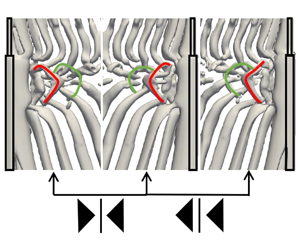
). Based on the order of their appearances, the green and red curves are named the NL-loop 1 and NL-loop 2, respectively.
$^{\prime }$
9–L10) form, and are indicated by green and red curves, respectively. Details of the formation processes of those loop structures were described in Tian et al. (Reference Tian, Jiang, Pettersen and Andersson2017a
). Based on the order of their appearances, the green and red curves are named the NL-loop 1 and NL-loop 2, respectively.

Figure 7. Schematic topology sketches illustrating the long-time history of the vortex connection topology and the vortex shedding. The thick black and grey straight lines represent vortices on the $-Y$
and
$-Y$
and $+Y$
sides, respectively. Only the N- and L-cell vortices are shown by short and long straight lines. The connections between them are depicted by thin solid curves. Black and grey solid curves indicate the connections between an N-cell vortex and its counterpart L-cell vortex. The red and green curves reveal different NL-loop structures (same colour code as used in figure 6). The dashed curves, on the other hand, indicate broken connections that are not able to persist due to dislocations. We define a new term ‘long N-cell cycle’ containing several conventional N-cell cycles, while the conventional N-cell cycle was firstly defined by Morton & Yarusevych (Reference Morton and Yarusevych2010b
) and adopted also in the present study.
$+Y$
sides, respectively. Only the N- and L-cell vortices are shown by short and long straight lines. The connections between them are depicted by thin solid curves. Black and grey solid curves indicate the connections between an N-cell vortex and its counterpart L-cell vortex. The red and green curves reveal different NL-loop structures (same colour code as used in figure 6). The dashed curves, on the other hand, indicate broken connections that are not able to persist due to dislocations. We define a new term ‘long N-cell cycle’ containing several conventional N-cell cycles, while the conventional N-cell cycle was firstly defined by Morton & Yarusevych (Reference Morton and Yarusevych2010b
) and adopted also in the present study.
Based on long-time observations ( $2500D/U$
), a schematic topology sketch is shown in figure 7. This will be used to introduce some important concepts. In figure 7, the short and long straight lines represent the N- and L-cell vortices, respectively. Between them, the curved solid lines connect the N-cell vortex and its counterpart L-cell vortex. The dashed curves indicate broken connections that are not able to persist due to dislocations. Detailed visualizations of vortex connections and dislocations in the first N-cell cycle are shown in figure 6. To ease the observation, we only show the connections between the N- and L-cell vortices. The L–L and N–N loops (Tian et al.
Reference Tian, Jiang, Pettersen and Andersson2017a
) are not shown in this figure.
$2500D/U$
), a schematic topology sketch is shown in figure 7. This will be used to introduce some important concepts. In figure 7, the short and long straight lines represent the N- and L-cell vortices, respectively. Between them, the curved solid lines connect the N-cell vortex and its counterpart L-cell vortex. The dashed curves indicate broken connections that are not able to persist due to dislocations. Detailed visualizations of vortex connections and dislocations in the first N-cell cycle are shown in figure 6. To ease the observation, we only show the connections between the N- and L-cell vortices. The L–L and N–N loops (Tian et al.
Reference Tian, Jiang, Pettersen and Andersson2017a
) are not shown in this figure.
We define the side of the N-cell vortex in an NL-loop structure as the side of the loop itself. For example, the NL-loop N8–L $^{\prime }$
9 (shown by green curves) in figure 6(g) is identified to form at the
$^{\prime }$
9 (shown by green curves) in figure 6(g) is identified to form at the $-Y$
side. As shown in figure 7, from the first to the seventh N-cell cycle, the NL-loop 1 (the green curves) appears alternately at the
$-Y$
side. As shown in figure 7, from the first to the seventh N-cell cycle, the NL-loop 1 (the green curves) appears alternately at the $+Y$
and
$+Y$
and $-Y$
side between subsequent N-cell cycles. This is what we called the antisymmetric vortex interactions in Tian et al. (Reference Tian, Jiang, Pettersen and Andersson2017a
). However, an unexpected interruption of this antisymmetry is observed between the seventh and eighth N-cell cycles. Figure 7 shows, in both the seventh and eighth N-cell cycles, that the NL-loop 1 appears at the
$-Y$
side between subsequent N-cell cycles. This is what we called the antisymmetric vortex interactions in Tian et al. (Reference Tian, Jiang, Pettersen and Andersson2017a
). However, an unexpected interruption of this antisymmetry is observed between the seventh and eighth N-cell cycles. Figure 7 shows, in both the seventh and eighth N-cell cycles, that the NL-loop 1 appears at the $-Y$
side (green curves connect to black short lines which represent the N-cell vortex on the
$-Y$
side (green curves connect to black short lines which represent the N-cell vortex on the $-Y$
side). We introduce the term ‘long N-cell cycle’ to identify the uninterrupted series of antisymmetric N-cell cycles. Within one long N-cell cycle, antisymmetric vortex interactions appear between subsequent N-cell cycles. However, at the boundary between two long N-cell cycles, this antisymmetry is interrupted. Our long-time observation covering eight long N-cell cycles shows that there are either seven or eight N-cell cycles in one long N-cell cycle. In fact, an exceptionally low frequency (
$-Y$
side). We introduce the term ‘long N-cell cycle’ to identify the uninterrupted series of antisymmetric N-cell cycles. Within one long N-cell cycle, antisymmetric vortex interactions appear between subsequent N-cell cycles. However, at the boundary between two long N-cell cycles, this antisymmetry is interrupted. Our long-time observation covering eight long N-cell cycles shows that there are either seven or eight N-cell cycles in one long N-cell cycle. In fact, an exceptionally low frequency ( $St_{1}$
) is captured in figure 5(b) where a power spectrum at position
$St_{1}$
) is captured in figure 5(b) where a power spectrum at position $(x/D,y/D,z/D)=(0.6,0.2,-4.4)$
is shown. The value of
$(x/D,y/D,z/D)=(0.6,0.2,-4.4)$
is shown. The value of $St_{1}$
is 0.0032, and is around
$St_{1}$
is 0.0032, and is around $St_{beat}/7.5$
. This coincides well with our observation that one long N-cell cycle contains either seven or eight N-cell cycles. We believe that this low-frequency component is related to the long N-cell cycles. More detailed information on this long-period phenomenon, and the unexpected interruption, will be discussed in § 5. The other visible frequency components in figure 5(b) are combinations of the basic frequency components, i.e.
$St_{beat}/7.5$
. This coincides well with our observation that one long N-cell cycle contains either seven or eight N-cell cycles. We believe that this low-frequency component is related to the long N-cell cycles. More detailed information on this long-period phenomenon, and the unexpected interruption, will be discussed in § 5. The other visible frequency components in figure 5(b) are combinations of the basic frequency components, i.e. $St_{S}$
,
$St_{S}$
, $St_{N}$
,
$St_{N}$
, $St_{L}$
and
$St_{L}$
and $St_{1}$
(Gerich & Eckelmann Reference Gerich and Eckelmann1982).
$St_{1}$
(Gerich & Eckelmann Reference Gerich and Eckelmann1982).
3.2 Necessity of monitoring the phase information of each N- and L-cell vortex
All the interesting physical phenomena, i.e. the formation of NL-loops, the unexpected interruption of the antisymmetry, etc., are directly related to the vortex dislocations in the wake behind the step cylinder. A consensus from the literature (Williamson Reference Williamson1989; Lewis & Gharib Reference Lewis and Gharib1992; Morton et al.
Reference Morton, Yarusevych and Carvajal-Mariscal2009) is that vortex dislocations are attributed to different shedding frequencies. In the present configuration, if both N- and L-cell vortices shed regularly, it is natural to directly use $f_{L}$
and
$f_{L}$
and $f_{N}$
to measure the phase difference (
$f_{N}$
to measure the phase difference ( $\unicode[STIX]{x1D6F7}$
) between N- and L-cell vortices. However, the actual wake flow is more complicated. In figure 8(a,b), we plot time traces of the instantaneous cross-flow velocity
$\unicode[STIX]{x1D6F7}$
) between N- and L-cell vortices. However, the actual wake flow is more complicated. In figure 8(a,b), we plot time traces of the instantaneous cross-flow velocity $v$
at two locations in the L- and N-cell regions in the symmetry plane. Two dashed sinusoidal curves with constant frequencies
$v$
at two locations in the L- and N-cell regions in the symmetry plane. Two dashed sinusoidal curves with constant frequencies $f_{L}$
and
$f_{L}$
and $f_{N}$
are also plotted in figure 8. By comparing figures 8(a) and (b), it is clear that, unlike the regularly shed L-cell vortices, the shedding frequency of the N-cell vortex slightly fluctuates during every N-cell cycle. This was also briefly mentioned by Morton & Yarusevych (Reference Morton and Yarusevych2010b
), but not investigated further. The irregularity of the N-cell shedding makes it challenging but necessary to monitor the phase information of every N-cell vortex. Therefore, we developed a method to obtain the phase information (
$f_{N}$
are also plotted in figure 8. By comparing figures 8(a) and (b), it is clear that, unlike the regularly shed L-cell vortices, the shedding frequency of the N-cell vortex slightly fluctuates during every N-cell cycle. This was also briefly mentioned by Morton & Yarusevych (Reference Morton and Yarusevych2010b
), but not investigated further. The irregularity of the N-cell shedding makes it challenging but necessary to monitor the phase information of every N-cell vortex. Therefore, we developed a method to obtain the phase information ( $\unicode[STIX]{x1D711}$
) and the phase difference (
$\unicode[STIX]{x1D711}$
) and the phase difference ( $\unicode[STIX]{x1D6F7}$
) of vortices. Details can be found in appendix A.
$\unicode[STIX]{x1D6F7}$
) of vortices. Details can be found in appendix A.

Figure 8. Time trace of the oscillating cross-flow velocity $v$
is plotted as the solid line: (a) at the sampling point
$v$
is plotted as the solid line: (a) at the sampling point $(x/D,y/D,z/D)=(1.4,0,-14.8)$
in the L-cell region, and (b) at the sampling point
$(x/D,y/D,z/D)=(1.4,0,-14.8)$
in the L-cell region, and (b) at the sampling point $(x/D,y/D,z/D)=(1.4,0,-2.8)$
in the N-cell region. For comparison, pure sinusoidal curves are plotted as dashed lines with frequency
$(x/D,y/D,z/D)=(1.4,0,-2.8)$
in the N-cell region. For comparison, pure sinusoidal curves are plotted as dashed lines with frequency $f_{L}$
in panel (a) and frequency
$f_{L}$
in panel (a) and frequency $f_{N}$
in panel (b);
$f_{N}$
in panel (b); $f_{L}$
and
$f_{L}$
and $f_{N}$
are calculated by FFT obtained from figure 5.
$f_{N}$
are calculated by FFT obtained from figure 5.
4 Two different phase difference accumulation mechanisms and their effects on vortex interactions
4.1 Two different phase difference accumulation mechanisms
From figure 6, one can see that both the N- and L-cell vortices are spanwise vortices. This means that the variation of the streamwise distance between corresponding N- and L-cell vortices can reflect the changes in their phase difference ( $\unicode[STIX]{x1D6F7}$
). In the present study, we use the location of the most concentrated spanwise vorticity (
$\unicode[STIX]{x1D6F7}$
). In the present study, we use the location of the most concentrated spanwise vorticity ( $\unicode[STIX]{x1D714}_{z}$
) to indicate the position of the corresponding vortex. In figure 9, we plot instantaneous spanwise vorticity
$\unicode[STIX]{x1D714}_{z}$
) to indicate the position of the corresponding vortex. In figure 9, we plot instantaneous spanwise vorticity $\unicode[STIX]{x1D714}_{z}$
contours at an
$\unicode[STIX]{x1D714}_{z}$
contours at an $(x,y)$
plane in the N-cell region
$(x,y)$
plane in the N-cell region $z/D=-2.9$
and L-cell region
$z/D=-2.9$
and L-cell region $z/D=-14$
. Four black lines indicate the positions of vortices N0 and L0. One can see that from
$z/D=-14$
. Four black lines indicate the positions of vortices N0 and L0. One can see that from $tU/D=4.5$
to 9, the streamwise distance between N0 and L0 increases from
$tU/D=4.5$
to 9, the streamwise distance between N0 and L0 increases from $1.8D$
(
$1.8D$
( $3.7D-1.9D$
) to
$3.7D-1.9D$
) to $2.3D$
(
$2.3D$
( $7.7D-5.4D$
) as they convect downstream. This means that, even after both N0 and L0 disconnect from the shear layer, as shown in figure 6(a),
$7.7D-5.4D$
) as they convect downstream. This means that, even after both N0 and L0 disconnect from the shear layer, as shown in figure 6(a), $\unicode[STIX]{x1D6F7}$
between them continues to accumulate. By marking the moment when the N-cell vortex just forms as an individual wake-type vortex, we divide the process of
$\unicode[STIX]{x1D6F7}$
between them continues to accumulate. By marking the moment when the N-cell vortex just forms as an individual wake-type vortex, we divide the process of $\unicode[STIX]{x1D6F7}$
accumulation into two parts. Before this moment,
$\unicode[STIX]{x1D6F7}$
accumulation into two parts. Before this moment, $\unicode[STIX]{x1D6F7}$
between the N- and L-cell vortex is dominated by their different shedding frequencies, called
$\unicode[STIX]{x1D6F7}$
between the N- and L-cell vortex is dominated by their different shedding frequencies, called $\unicode[STIX]{x1D6F7}_{f}$
. After this moment,
$\unicode[STIX]{x1D6F7}_{f}$
. After this moment, $\unicode[STIX]{x1D6F7}$
is caused by different convective velocities in the N- and L-cell regions, and called
$\unicode[STIX]{x1D6F7}$
is caused by different convective velocities in the N- and L-cell regions, and called $\unicode[STIX]{x1D6F7}_{c}$
. Detailed descriptions of monitoring
$\unicode[STIX]{x1D6F7}_{c}$
. Detailed descriptions of monitoring $\unicode[STIX]{x1D6F7}_{f}$
and
$\unicode[STIX]{x1D6F7}_{f}$
and $\unicode[STIX]{x1D711}$
can be found in appendix A. Owing to the spatial inhomogeneity of the convective velocity, it is difficult to accurately assess its effect on
$\unicode[STIX]{x1D711}$
can be found in appendix A. Owing to the spatial inhomogeneity of the convective velocity, it is difficult to accurately assess its effect on $\unicode[STIX]{x1D6F7}$
. Yet, the distributions of mean streamwise velocity (
$\unicode[STIX]{x1D6F7}$
. Yet, the distributions of mean streamwise velocity ( $\bar{u}$
) in different vortex cell regions can roughly indicate the influence.
$\bar{u}$
) in different vortex cell regions can roughly indicate the influence.

Figure 9. Instantaneous spanwise vorticity $\unicode[STIX]{x1D714}_{z}$
(
$\unicode[STIX]{x1D714}_{z}$
( $\unicode[STIX]{x1D714}_{z}=\unicode[STIX]{x2202}v/\unicode[STIX]{x2202}x-\unicode[STIX]{x2202}u/\unicode[STIX]{x2202}y$
) contour plots in an (
$\unicode[STIX]{x1D714}_{z}=\unicode[STIX]{x2202}v/\unicode[STIX]{x2202}x-\unicode[STIX]{x2202}u/\unicode[STIX]{x2202}y$
) contour plots in an ( $x,y$
) plane in (a,c) the N-cell region
$x,y$
) plane in (a,c) the N-cell region $z/D=-2.9$
(black solid line in figure 6(a,b)) and (b,d) in the L-cell region
$z/D=-2.9$
(black solid line in figure 6(a,b)) and (b,d) in the L-cell region $z/D=-14$
(black dotted line in figure 6(a,b)). By detecting the location of concentrated vorticity, the positions of vortices N
$z/D=-14$
(black dotted line in figure 6(a,b)). By detecting the location of concentrated vorticity, the positions of vortices N $^{\prime }$
9 and L
$^{\prime }$
9 and L $^{\prime }$
9 are marked by black lines. (Note that we have compared the position of the centre of the concentrated vorticity and the centre in the region defined by
$^{\prime }$
9 are marked by black lines. (Note that we have compared the position of the centre of the concentrated vorticity and the centre in the region defined by $\unicode[STIX]{x1D706}_{2}$
isolines, and confirmed only tiny differences.)
$\unicode[STIX]{x1D706}_{2}$
isolines, and confirmed only tiny differences.)

Figure 10. (a) Distributions of the mean streamwise velocity ( $\overline{u}/U$
) along spanwise lines with the same
$\overline{u}/U$
) along spanwise lines with the same $x$
-coordinate (
$x$
-coordinate ( $x/D=1.6$
), but for different
$x/D=1.6$
), but for different $y$
-coordinates. (b) Distributions of mean streamwise velocity
$y$
-coordinates. (b) Distributions of mean streamwise velocity $\bar{u}/U$
along spanwise lines with different
$\bar{u}/U$
along spanwise lines with different $x$
-coordinates in the symmetry plane (
$x$
-coordinates in the symmetry plane ( $y/D=0$
).
$y/D=0$
).
In figure 10, the spanwise distributions of $\bar{u}$
are plotted at several downstream positions. As shown in figure 10(a), the mean streamwise velocity in the N-cell region in the symmetry plane
$\bar{u}$
are plotted at several downstream positions. As shown in figure 10(a), the mean streamwise velocity in the N-cell region in the symmetry plane $(y/D=0)$
is nearly 0.2
$(y/D=0)$
is nearly 0.2 $U$
less than that in the L-cell region. At the side plane
$U$
less than that in the L-cell region. At the side plane $y/D=0.8$
, this difference still reaches 0.1
$y/D=0.8$
, this difference still reaches 0.1 $U$
. From figure 10(b), we see that the difference in mean streamwise velocity is clear until a downstream position
$U$
. From figure 10(b), we see that the difference in mean streamwise velocity is clear until a downstream position $x/D=4$
. In other words, at least until
$x/D=4$
. In other words, at least until $x/D=4$
in the wake, the convective velocity distribution is distinctly non-uniform in the spanwise direction. This non-uniformity induces an additional
$x/D=4$
in the wake, the convective velocity distribution is distinctly non-uniform in the spanwise direction. This non-uniformity induces an additional $\unicode[STIX]{x1D6F7}$
when the vortices convect downstream. We note that this role of the non-uniform convection velocity and its effects have never been addressed before.
$\unicode[STIX]{x1D6F7}$
when the vortices convect downstream. We note that this role of the non-uniform convection velocity and its effects have never been addressed before.
4.2 Effects of two phase difference accumulation mechanisms
4.2.1 Differences in formation positions of the NL-loop 1 and NL-loop 2
The formation process of the NL-loop 1 in each N-cell cycle is repetitive. An example of this process is presented in figure 11, where the vortex structures are shown from both $+Y$
and
$+Y$
and $-Y$
sides of the step cylinder. In figure 11(a,b), and the corresponding zoom-in plots (figure 11
f,g), the foot of vortex N8 completely disconnects from the shear layer at
$-Y$
sides of the step cylinder. In figure 11(a,b), and the corresponding zoom-in plots (figure 11
f,g), the foot of vortex N8 completely disconnects from the shear layer at $x/D=2.8$
(marked by a black line in figure 11(b,g)). At this moment (
$x/D=2.8$
(marked by a black line in figure 11(b,g)). At this moment ( $tU/D=33.3$
) the NL-loop 1 structure has not yet formed, because there is still no direct connection between N8 and L
$tU/D=33.3$
) the NL-loop 1 structure has not yet formed, because there is still no direct connection between N8 and L $^{\prime }$
9. It takes some more time for N8 to convect downstream and eventually develop into the NL-loop 1 with L
$^{\prime }$
9. It takes some more time for N8 to convect downstream and eventually develop into the NL-loop 1 with L $^{\prime }$
9 at
$^{\prime }$
9 at $x/D=3.3$
and
$x/D=3.3$
and $tU/D=34.5$
. This process is indicated in figure 11(b–e) and the corresponding zoom-in plots (figure 11
g–j). By following the same process as described in § 4.1, we found that from
$tU/D=34.5$
. This process is indicated in figure 11(b–e) and the corresponding zoom-in plots (figure 11
g–j). By following the same process as described in § 4.1, we found that from $tU/D=33.3$
to 34.5, the streamwise distance between vortex N
$tU/D=33.3$
to 34.5, the streamwise distance between vortex N $^{\prime }$
9 and L
$^{\prime }$
9 and L $^{\prime }$
9 increases from
$^{\prime }$
9 increases from $5.3D$
to
$5.3D$
to $6.1D$
as they move downstream. When
$6.1D$
as they move downstream. When $\unicode[STIX]{x1D6F7}$
between vortex N
$\unicode[STIX]{x1D6F7}$
between vortex N $^{\prime }$
9 and L
$^{\prime }$
9 and L $^{\prime }$
9 increases, L
$^{\prime }$
9 increases, L $^{\prime }$
9 gradually disconnects from its counterpart N
$^{\prime }$
9 gradually disconnects from its counterpart N $^{\prime }$
9 and forms the NL-loop 1 with N8 (see figure 11
k–o).
$^{\prime }$
9 and forms the NL-loop 1 with N8 (see figure 11
k–o).

Figure 11. The formation process of the NL-loop 1 structure in the first dislocation process (defined in figure 7) is shown from the $-Y$
and
$-Y$
and $+Y$
sides in (a–e) and (k–o) rows, respectively. In (f–j), zoom-in plots of vortex structures at N-cell region (black rectangle in panel a) are shown. The black circles highlight the position where the NL-loop 1 forms.
$+Y$
sides in (a–e) and (k–o) rows, respectively. In (f–j), zoom-in plots of vortex structures at N-cell region (black rectangle in panel a) are shown. The black circles highlight the position where the NL-loop 1 forms.

Figure 12. The formation process of the NL-loop 2 structure in the first dislocation process is shown from both $+Y$
and
$+Y$
and $-Y$
sides. The black circles highlight the position where the NL-loop 2 structure is formed.
$-Y$
sides. The black circles highlight the position where the NL-loop 2 structure is formed.
Unlike the NL-loop 1 structure, which has a distinct formation position, it is difficult to pinpoint where the NL-loop 2 forms. As shown in figure 12(a–e), in the black circle area, it is not clear how the foot of vortex N $^{\prime }$
9 completely separates from the shear layer and subsequently connects to L10 as they move downstream. The connection between N
$^{\prime }$
9 completely separates from the shear layer and subsequently connects to L10 as they move downstream. The connection between N $^{\prime }$
9 and L10 forms in the very near wake before N
$^{\prime }$
9 and L10 forms in the very near wake before N $^{\prime }$
9 completely disconnects from the shear layer. In order to compare with the formation process of the NL-loop 1 structure shown in figure 11, we use the same method to monitor the variation of the streamwise distance between vortices N10 and L10. At
$^{\prime }$
9 completely disconnects from the shear layer. In order to compare with the formation process of the NL-loop 1 structure shown in figure 11, we use the same method to monitor the variation of the streamwise distance between vortices N10 and L10. At $tU/D=36.9$
(the corresponding instantaneous isosurface of the vortex structure is shown in figure 12(g)), the distance between vortex N10 and L10 reaches
$tU/D=36.9$
(the corresponding instantaneous isosurface of the vortex structure is shown in figure 12(g)), the distance between vortex N10 and L10 reaches $5.9D$
. This is very close to the distance between N
$5.9D$
. This is very close to the distance between N $^{\prime }$
9 and L
$^{\prime }$
9 and L $^{\prime }$
9 at
$^{\prime }$
9 at $tU/D=34.5$
(figure 11
n), when L
$tU/D=34.5$
(figure 11
n), when L $^{\prime }$
9 successfully induces N8 to connect to itself and together form the NL-loop 1 structure. At
$^{\prime }$
9 successfully induces N8 to connect to itself and together form the NL-loop 1 structure. At $tU/D=36.9$
, as shown in figure 12(b), the leg of vortex N
$tU/D=36.9$
, as shown in figure 12(b), the leg of vortex N $^{\prime }$
9 is at position
$^{\prime }$
9 is at position $x/D=2.8$
. At the same downstream position, the foot of vortex N8 already disconnects from the shear layer, as shown in figure 11(b). It is reasonable to speculate that
$x/D=2.8$
. At the same downstream position, the foot of vortex N8 already disconnects from the shear layer, as shown in figure 11(b). It is reasonable to speculate that $\unicode[STIX]{x1D6F7}$
between N10 and L10 becomes sufficiently large to attract N
$\unicode[STIX]{x1D6F7}$
between N10 and L10 becomes sufficiently large to attract N $^{\prime }$
9 to connect to L10 before it disconnects from the shear layer. As a consequence, the formation position of NL-loop 2 is not so clear.
$^{\prime }$
9 to connect to L10 before it disconnects from the shear layer. As a consequence, the formation position of NL-loop 2 is not so clear.

Figure 13. (a) Time trace of $\unicode[STIX]{x1D6F7}_{f}$
between corresponding N-cell and L-cell vortices in the first (LNC1) and second (LNC2) long N-cell cycles, i.e. from the first to the 15th N-cell cycle. The circles represent
$\unicode[STIX]{x1D6F7}_{f}$
between corresponding N-cell and L-cell vortices in the first (LNC1) and second (LNC2) long N-cell cycles, i.e. from the first to the 15th N-cell cycle. The circles represent $\unicode[STIX]{x1D6F7}_{f}$
between an N-cell vortex and its counterpart L-cell vortex. The green and red circles indicate
$\unicode[STIX]{x1D6F7}_{f}$
between an N-cell vortex and its counterpart L-cell vortex. The green and red circles indicate $\unicode[STIX]{x1D6F7}_{f}$
, which eventually causes formation of the NL-loop 1 and NL-loop 2 structures, respectively. From the first to the eighth N-cell cycle, the green and red circles are numbered. (b) A zoom-in plot of the time trace of
$\unicode[STIX]{x1D6F7}_{f}$
, which eventually causes formation of the NL-loop 1 and NL-loop 2 structures, respectively. From the first to the eighth N-cell cycle, the green and red circles are numbered. (b) A zoom-in plot of the time trace of $\unicode[STIX]{x1D6F7}_{f}$
in the first N-cell cycle (the black dashed rectangle in panel a). From the left to the right, circles represent
$\unicode[STIX]{x1D6F7}_{f}$
in the first N-cell cycle (the black dashed rectangle in panel a). From the left to the right, circles represent $\unicode[STIX]{x1D6F7}_{f}$
between the vortex pair N
$\unicode[STIX]{x1D6F7}_{f}$
between the vortex pair N $^{\prime }$
1–L
$^{\prime }$
1–L $^{\prime }$
1 to the vortex pair N10–L10, respectively. (Note that the detailed calculation processes can be found in appendix A. All detailed data about
$^{\prime }$
1 to the vortex pair N10–L10, respectively. (Note that the detailed calculation processes can be found in appendix A. All detailed data about $\unicode[STIX]{x1D6F7}_{f}$
and the longer-time trace of
$\unicode[STIX]{x1D6F7}_{f}$
and the longer-time trace of $\unicode[STIX]{x1D6F7}_{f}$
are included in the supplementary material, file 1, available at https://doi.org/10.1017/jfm.2020.110. The trigger value and the threshold value are estimated based on 55 N-cell cycles, as shown in supplementary file 3.)
$\unicode[STIX]{x1D6F7}_{f}$
are included in the supplementary material, file 1, available at https://doi.org/10.1017/jfm.2020.110. The trigger value and the threshold value are estimated based on 55 N-cell cycles, as shown in supplementary file 3.)

Figure 14. The just-formed NL-loop 1 structures in the first to the eighth N-cell cycle are plotted from both the $-Y$
and
$-Y$
and $+Y$
sides (the first long N-cell cycle consists of the first to the seventh N-cell cycles). The black line marks the formation position of NL-loop 1. The red circle in panel (f) highlights an irregular absence of the NL-loop 1 structure, which will be discussed later.
$+Y$
sides (the first long N-cell cycle consists of the first to the seventh N-cell cycles). The black line marks the formation position of NL-loop 1. The red circle in panel (f) highlights an irregular absence of the NL-loop 1 structure, which will be discussed later.
The time trace of $\unicode[STIX]{x1D6F7}_{f}$
accumulation proves our speculation. By using the method described in appendix A, the time trace of
$\unicode[STIX]{x1D6F7}_{f}$
accumulation proves our speculation. By using the method described in appendix A, the time trace of $\unicode[STIX]{x1D6F7}_{f}$
accumulation in the first N-cell cycle is shown in figure 13(b). Circles in this figure represent
$\unicode[STIX]{x1D6F7}_{f}$
accumulation in the first N-cell cycle is shown in figure 13(b). Circles in this figure represent $\unicode[STIX]{x1D6F7}_{f}$
of corresponding N- and L-cell vortices, in which the green circle represents
$\unicode[STIX]{x1D6F7}_{f}$
of corresponding N- and L-cell vortices, in which the green circle represents $\unicode[STIX]{x1D6F7}_{f}$
between N
$\unicode[STIX]{x1D6F7}_{f}$
between N $^{\prime }$
9 and L
$^{\prime }$
9 and L $^{\prime }$
9, and the red circle represents
$^{\prime }$
9, and the red circle represents $\unicode[STIX]{x1D6F7}_{f}$
between N10 and L10. Eventually, the dislocations of the vortex pairs corresponding to the green and red circles cause formation of the NL-loop 1 structure (N8–L
$\unicode[STIX]{x1D6F7}_{f}$
between N10 and L10. Eventually, the dislocations of the vortex pairs corresponding to the green and red circles cause formation of the NL-loop 1 structure (N8–L $^{\prime }$
9) and the NL-loop 2 structure (N
$^{\prime }$
9) and the NL-loop 2 structure (N $^{\prime }$
9–L10), respectively.
$^{\prime }$
9–L10), respectively.
One can see that the red circle represents a larger $\unicode[STIX]{x1D6F7}_{f}$
value than the green one, which means that
$\unicode[STIX]{x1D6F7}_{f}$
value than the green one, which means that $\unicode[STIX]{x1D6F7}_{f}$
between N10 and L10 is larger than that between N
$\unicode[STIX]{x1D6F7}_{f}$
between N10 and L10 is larger than that between N $^{\prime }$
9 and L
$^{\prime }$
9 and L $^{\prime }$
9. Therefore, compared to the vortex pair N10–L10, the vortex pair N
$^{\prime }$
9. Therefore, compared to the vortex pair N10–L10, the vortex pair N $^{\prime }$
9–L
$^{\prime }$
9–L $^{\prime }$
9 needs a larger contribution of
$^{\prime }$
9 needs a larger contribution of $\unicode[STIX]{x1D6F7}_{c}$
to achieve a sufficiently large
$\unicode[STIX]{x1D6F7}_{c}$
to achieve a sufficiently large $\unicode[STIX]{x1D6F7}$
to trigger the vortex dislocation between them, and the subsequent formation of the NL-loop 1 (N8–L
$\unicode[STIX]{x1D6F7}$
to trigger the vortex dislocation between them, and the subsequent formation of the NL-loop 1 (N8–L $^{\prime }$
9). In other words, due to the reduced need of a contribution from
$^{\prime }$
9). In other words, due to the reduced need of a contribution from $\unicode[STIX]{x1D6F7}_{c}$
, the vortex dislocation between N10 and L10 and the subsequent NL-loop 2 (N
$\unicode[STIX]{x1D6F7}_{c}$
, the vortex dislocation between N10 and L10 and the subsequent NL-loop 2 (N $^{\prime }$
9–L10) is formed closer to the cylinder, which causes the unclear formation position.
$^{\prime }$
9–L10) is formed closer to the cylinder, which causes the unclear formation position.
4.2.2 Variation of formation positions of the NL-loop 1 structures
In figure 14, the NL-loop 1 structures in the first eight N-cell cycles are plotted. The black vertical lines show the positions where the NL-loop 1 structures just form. Except for the sixth N-cell cycle (figure 14
f), the NL-loop 1 structures alternately appear at the $+Y$
and
$+Y$
and $-Y$
side of the step cylinder from the first to the seventh N-cell cycles (the first long N-cell cycle). The shape and the formation position of the NL-loop 1 structure also vary, as depicted in figure 14(a–h).
$-Y$
side of the step cylinder from the first to the seventh N-cell cycles (the first long N-cell cycle). The shape and the formation position of the NL-loop 1 structure also vary, as depicted in figure 14(a–h).

Figure 15. Relation between $\unicode[STIX]{x1D6F7}_{f}$
and the formation position
$\unicode[STIX]{x1D6F7}_{f}$
and the formation position $(x/D)$
of corresponding NL-loop 1 structures in the first to the seventh long N-cell cycles (52 N-cell cycles are included). Based on the trends of the curves, one stable range and two unstable ranges are identified. A straight dashed line outlines the trend of the stable range. The occasionally absent NL-loop 1 structures in these seven long N-cell cycles are marked by red colour at the expected formation positions, which can be obtained by linear interpolation.
$(x/D)$
of corresponding NL-loop 1 structures in the first to the seventh long N-cell cycles (52 N-cell cycles are included). Based on the trends of the curves, one stable range and two unstable ranges are identified. A straight dashed line outlines the trend of the stable range. The occasionally absent NL-loop 1 structures in these seven long N-cell cycles are marked by red colour at the expected formation positions, which can be obtained by linear interpolation.
Table 3. Formation positions and $\unicode[STIX]{x1D6F7}_{f}$
values that cause the NL-loop 1 structures in the first to seventh N-cell cycle (the first long N-cell cycle). The corresponding vortex structures are shown in figure 14(a–g). In the sixth N-cell cycle, there is a loop formation failure.
$\unicode[STIX]{x1D6F7}_{f}$
values that cause the NL-loop 1 structures in the first to seventh N-cell cycle (the first long N-cell cycle). The corresponding vortex structures are shown in figure 14(a–g). In the sixth N-cell cycle, there is a loop formation failure.

In table 3, the relation between the formation positions of the NL-loop 1 structures in the first long N-cell cycle and their $\unicode[STIX]{x1D6F7}_{f}$
are presented. One can see that, except for the sixth N-cell cycle, the formation positions move downstream as the corresponding
$\unicode[STIX]{x1D6F7}_{f}$
are presented. One can see that, except for the sixth N-cell cycle, the formation positions move downstream as the corresponding $\unicode[STIX]{x1D6F7}_{f}$
decreases. This can easily be ascribed to the already discussed two different phase difference accumulation mechanisms. Formation of the NL-loop 1 structures requires sufficiently large
$\unicode[STIX]{x1D6F7}_{f}$
decreases. This can easily be ascribed to the already discussed two different phase difference accumulation mechanisms. Formation of the NL-loop 1 structures requires sufficiently large $\unicode[STIX]{x1D6F7}$
. Since
$\unicode[STIX]{x1D6F7}$
. Since $\unicode[STIX]{x1D6F7}_{f}$
decreases,
$\unicode[STIX]{x1D6F7}_{f}$
decreases, $\unicode[STIX]{x1D6F7}_{c}$
must contribute more, which consequently leads to a longer formation time and further downstream formation position. To be more clear, the relations between
$\unicode[STIX]{x1D6F7}_{c}$
must contribute more, which consequently leads to a longer formation time and further downstream formation position. To be more clear, the relations between $\unicode[STIX]{x1D6F7}_{f}$
and formation positions of the corresponding NL-loop 1 structures during the first–seventh long N-cell cycles are plotted in figure 15. Generally, except for several irregular points, the formation position shifts downstream as
$\unicode[STIX]{x1D6F7}_{f}$
and formation positions of the corresponding NL-loop 1 structures during the first–seventh long N-cell cycles are plotted in figure 15. Generally, except for several irregular points, the formation position shifts downstream as $\unicode[STIX]{x1D6F7}_{f}$
decreases. (Note that the appearances of the irregular points will be discussed in § 5.3.)
$\unicode[STIX]{x1D6F7}_{f}$
decreases. (Note that the appearances of the irregular points will be discussed in § 5.3.)
Based on the discussions above, we conclude that, for the NL-loop structures, $\unicode[STIX]{x1D6F7}$
is accumulated by the joint influence of different shedding frequencies and different convective velocities
$\unicode[STIX]{x1D6F7}$
is accumulated by the joint influence of different shedding frequencies and different convective velocities
 $$\begin{eqnarray}\unicode[STIX]{x1D6F7}=\unicode[STIX]{x1D6F7}_{f}+\unicode[STIX]{x1D6F7}_{c}.\end{eqnarray}$$
As the relative magnitude of $\unicode[STIX]{x1D6F7}_{f}$
and
$\unicode[STIX]{x1D6F7}_{f}$
and $\unicode[STIX]{x1D6F7}_{c}$
varies, the formation processes of the NL-loop structures change.
$\unicode[STIX]{x1D6F7}_{c}$
varies, the formation processes of the NL-loop structures change.
5 Characteristics of the long N-cell cycles
5.1 Trend of
$\unicode[STIX]{x1D6F7}_{f}$
variation

The time trace of $\unicode[STIX]{x1D6F7}_{f}$
accumulation between corresponding N- and L-cell vortices is plotted in figure 13(a). We use green and red circles to indicate
$\unicode[STIX]{x1D6F7}_{f}$
accumulation between corresponding N- and L-cell vortices is plotted in figure 13(a). We use green and red circles to indicate $\unicode[STIX]{x1D6F7}_{f}$
of the pair of N- and L-cell vortices whose dislocation eventually causes the NL-loop 1 and NL-loop 2, respectively. Two solid lines with the same corresponding colours describe the decreasing tendency in
$\unicode[STIX]{x1D6F7}_{f}$
of the pair of N- and L-cell vortices whose dislocation eventually causes the NL-loop 1 and NL-loop 2, respectively. Two solid lines with the same corresponding colours describe the decreasing tendency in $\unicode[STIX]{x1D6F7}_{f}$
of both NL-loop 1 and NL-loop 2 over time.
$\unicode[STIX]{x1D6F7}_{f}$
of both NL-loop 1 and NL-loop 2 over time.
The gradual decrease of $\unicode[STIX]{x1D6F7}_{f}$
in each N-cell cycle can be expressed as
$\unicode[STIX]{x1D6F7}_{f}$
in each N-cell cycle can be expressed as
 $$\begin{eqnarray}S=\unicode[STIX]{x1D6FC}\frac{1}{2\,f_{L}}-\unicode[STIX]{x1D6FD}\frac{1}{2\,f_{N}},\end{eqnarray}$$
where $S$
(with dimension
$S$
(with dimension $D/U$
) is a measure of the phase shift of every vortex pair in one N-cell cycle, as compared to the N-cell cycle before it. In this expression,
$D/U$
) is a measure of the phase shift of every vortex pair in one N-cell cycle, as compared to the N-cell cycle before it. In this expression, $\unicode[STIX]{x1D6FC}$
and
$\unicode[STIX]{x1D6FC}$
and $\unicode[STIX]{x1D6FD}$
represent the number of L- and N-cell vortices in one N-cell cycle; and
$\unicode[STIX]{x1D6FD}$
represent the number of L- and N-cell vortices in one N-cell cycle; and $f_{L}$
and
$f_{L}$
and $f_{N}$
are the shedding frequencies of L- and N-cell vortices. In the present case,
$f_{N}$
are the shedding frequencies of L- and N-cell vortices. In the present case, $\unicode[STIX]{x1D6FC}=15$
,
$\unicode[STIX]{x1D6FC}=15$
, $\unicode[STIX]{x1D6FD}=13$
,
$\unicode[STIX]{x1D6FD}=13$
, $f_{L}D/U=0.1780$
and
$f_{L}D/U=0.1780$
and $f_{N}D/U=0.1545$
(from figure 5), from which we obtain
$f_{N}D/U=0.1545$
(from figure 5), from which we obtain $S=0.064D/U$
. This means that, in one N-cell cycle, the duration of 13 N-cell and 15 L-cell vortices is not exactly the same. Although
$S=0.064D/U$
. This means that, in one N-cell cycle, the duration of 13 N-cell and 15 L-cell vortices is not exactly the same. Although $S$
has a very small value, after a certain number of N-cell cycles, the accumulated difference becomes large enough to influence the dislocation process. Moreover, by checking figure 13(a) and the supplementary file 1, one can find that from R1 to R7 or from G1 to G7,
$S$
has a very small value, after a certain number of N-cell cycles, the accumulated difference becomes large enough to influence the dislocation process. Moreover, by checking figure 13(a) and the supplementary file 1, one can find that from R1 to R7 or from G1 to G7, $\unicode[STIX]{x1D6F7}_{f}$
decreases by approximately 0.4
$\unicode[STIX]{x1D6F7}_{f}$
decreases by approximately 0.4 $D/U$
, i.e.
$D/U$
, i.e. $\unicode[STIX]{x1D6F7}_{f}$
decreases by around 0.067
$\unicode[STIX]{x1D6F7}_{f}$
decreases by around 0.067 $D/U$
after every N-cell cycle, which is close to the
$D/U$
after every N-cell cycle, which is close to the $S$
value from expression (5.1).
$S$
value from expression (5.1).
It is worth mentioning that the numbers $\unicode[STIX]{x1D6FC}=15$
,
$\unicode[STIX]{x1D6FC}=15$
, $\unicode[STIX]{x1D6FD}=13$
and
$\unicode[STIX]{x1D6FD}=13$
and $S=0.064D/U$
are related to the particular configuration studied. For different configurations, i.e. different
$S=0.064D/U$
are related to the particular configuration studied. For different configurations, i.e. different $D/d$
and
$D/d$
and $Re_{D}$
, these numbers in expression (5.1) may vary. But what we observe in figure 13(a) will be a common feature, because it is extremely unlikely to attain an
$Re_{D}$
, these numbers in expression (5.1) may vary. But what we observe in figure 13(a) will be a common feature, because it is extremely unlikely to attain an $S$
value exactly equal to zero.
$S$
value exactly equal to zero.
5.2 Interruption of the antisymmetric phenomenon
From figure 14(a–h), one can clearly see that the NL-loop 1 structure alternately appears at the $-Y$
and
$-Y$
and $+Y$
side of the step cylinder in subsequent N-cell cycles. This is the antisymmetric phenomenon reported in Tian et al. (Reference Tian, Jiang, Pettersen and Andersson2017a
). In the present case, the long-time observation reveals that this antisymmetric phenomenon will be interrupted once in a while. As shown in figure 14(g,h), instead of being antisymmetric, the loop structures in the seventh and eighth N-cell cycles are symmetric. In these two N-cell cycles, both NL-loop 1 structures, i.e. N86–L
$+Y$
side of the step cylinder in subsequent N-cell cycles. This is the antisymmetric phenomenon reported in Tian et al. (Reference Tian, Jiang, Pettersen and Andersson2017a
). In the present case, the long-time observation reveals that this antisymmetric phenomenon will be interrupted once in a while. As shown in figure 14(g,h), instead of being antisymmetric, the loop structures in the seventh and eighth N-cell cycles are symmetric. In these two N-cell cycles, both NL-loop 1 structures, i.e. N86–L $^{\prime }$
99 and N100–L
$^{\prime }$
99 and N100–L $^{\prime }$
115, are formed at the
$^{\prime }$
115, are formed at the $-Y$
side.
$-Y$
side.
This interruption is caused by the decreasing tendency in $\unicode[STIX]{x1D6F7}_{f}$
, as we discussed in § 5.1. Normally, there are 13 N-cell and 15 L-cell vortices in one N-cell cycle. The odd number of N-cell vortices causes the antisymmetric phenomenon. However, as shown in figure 13(a), when
$\unicode[STIX]{x1D6F7}_{f}$
, as we discussed in § 5.1. Normally, there are 13 N-cell and 15 L-cell vortices in one N-cell cycle. The odd number of N-cell vortices causes the antisymmetric phenomenon. However, as shown in figure 13(a), when $\unicode[STIX]{x1D6F7}_{f}$
continues to decrease along the green line from G1 to C8, it eventually becomes insufficient in point C8. Even by including the contribution of
$\unicode[STIX]{x1D6F7}_{f}$
continues to decrease along the green line from G1 to C8, it eventually becomes insufficient in point C8. Even by including the contribution of $\unicode[STIX]{x1D6F7}_{c}$
,
$\unicode[STIX]{x1D6F7}_{c}$
, $\unicode[STIX]{x1D6F7}$
is still not large enough to induce the formation of the expected NL-loop 1 (N
$\unicode[STIX]{x1D6F7}$
is still not large enough to induce the formation of the expected NL-loop 1 (N $^{\prime }$
99–L114). Therefore, in this N-cell cycle, one additional vortex pair shedding is needed to make
$^{\prime }$
99–L114). Therefore, in this N-cell cycle, one additional vortex pair shedding is needed to make $\unicode[STIX]{x1D6F7}$
sufficiently large to induce formation of the NL-loop 1. The additional one pair of N- and L-cell vortices makes the number of N-cell vortices in the eighth N-cell cycle become even, and thereby interrupts the antisymmetric phenomenon. In the supplementary file 3, the time trace of
$\unicode[STIX]{x1D6F7}$
sufficiently large to induce formation of the NL-loop 1. The additional one pair of N- and L-cell vortices makes the number of N-cell vortices in the eighth N-cell cycle become even, and thereby interrupts the antisymmetric phenomenon. In the supplementary file 3, the time trace of $\unicode[STIX]{x1D6F7}_{f}$
between N- and L-cell vortices in the first to the eighth long N-cell cycles (the first to the 55th N-cell cycles) is illustrated.
$\unicode[STIX]{x1D6F7}_{f}$
between N- and L-cell vortices in the first to the eighth long N-cell cycles (the first to the 55th N-cell cycles) is illustrated.
5.3 Trigger value and threshold value of vortex dislocations
Based on the results from earlier papers (Williamson Reference Williamson1989; Morton & Yarusevych Reference Morton and Yarusevych2010b
) and our discussions in §§ 5.2 and 4, it is clear that only when $\unicode[STIX]{x1D6F7}$
becomes sufficiently large can the vortex dislocation process be triggered. We call this value the ‘trigger value’. Based on (4.1),
$\unicode[STIX]{x1D6F7}$
becomes sufficiently large can the vortex dislocation process be triggered. We call this value the ‘trigger value’. Based on (4.1), $\unicode[STIX]{x1D6F7}$
consists of two parts,
$\unicode[STIX]{x1D6F7}$
consists of two parts, $\unicode[STIX]{x1D6F7}_{f}$
and
$\unicode[STIX]{x1D6F7}_{f}$
and $\unicode[STIX]{x1D6F7}_{c}$
. Owing to the complexity of
$\unicode[STIX]{x1D6F7}_{c}$
. Owing to the complexity of $\unicode[STIX]{x1D6F7}_{c}$
, an accurate trigger value is hard to obtain, but an approximate value is possible to estimate. As we discussed in § 4, unlike the NL-loop 1 structure, which has a clear formation position, the NL-loop 2 structure forms in the near wake. This makes it hard to define the exact formation position of the NL-loop 2. It means that the
$\unicode[STIX]{x1D6F7}_{c}$
, an accurate trigger value is hard to obtain, but an approximate value is possible to estimate. As we discussed in § 4, unlike the NL-loop 1 structure, which has a clear formation position, the NL-loop 2 structure forms in the near wake. This makes it hard to define the exact formation position of the NL-loop 2. It means that the $\unicode[STIX]{x1D6F7}_{f}$
that induces this NL-loop 2 is very close to the trigger value, and only a modest contribution from
$\unicode[STIX]{x1D6F7}_{f}$
that induces this NL-loop 2 is very close to the trigger value, and only a modest contribution from $\unicode[STIX]{x1D6F7}_{c}$
is needed. Therefore, by considering all the largest
$\unicode[STIX]{x1D6F7}_{c}$
is needed. Therefore, by considering all the largest $\unicode[STIX]{x1D6F7}_{f}$
corresponding to the NL-loop 2 structures, we can draw the blue line in figure 13(a) to approximate the trigger value (around 5.60
$\unicode[STIX]{x1D6F7}_{f}$
corresponding to the NL-loop 2 structures, we can draw the blue line in figure 13(a) to approximate the trigger value (around 5.60 $D/U$
).
$D/U$
).
Besides the trigger value, there is another interesting value of $\unicode[STIX]{x1D6F7}_{f}$
that should be noted. As we discussed in § 5.2, when
$\unicode[STIX]{x1D6F7}_{f}$
that should be noted. As we discussed in § 5.2, when $\unicode[STIX]{x1D6F7}_{f}$
continues to decrease from G1 to C8 (figure 13
a), the expected formation of the NL-loop 1 (N
$\unicode[STIX]{x1D6F7}_{f}$
continues to decrease from G1 to C8 (figure 13
a), the expected formation of the NL-loop 1 (N $^{\prime }$
99–L118) fails. We can speculate that there is a threshold value for
$^{\prime }$
99–L118) fails. We can speculate that there is a threshold value for $\unicode[STIX]{x1D6F7}_{f}$
, such that when
$\unicode[STIX]{x1D6F7}_{f}$
, such that when $\unicode[STIX]{x1D6F7}_{f}$
becomes less than this value, a vortex dislocation will not occur, even when taking the contribution from
$\unicode[STIX]{x1D6F7}_{f}$
becomes less than this value, a vortex dislocation will not occur, even when taking the contribution from $\unicode[STIX]{x1D6F7}_{c}$
into account. By connecting all of the smallest values of
$\unicode[STIX]{x1D6F7}_{c}$
into account. By connecting all of the smallest values of $\unicode[STIX]{x1D6F7}_{f}$
in green (
$\unicode[STIX]{x1D6F7}_{f}$
in green ( $\unicode[STIX]{x1D6F7}_{f}$
inducing the NL-loop 1), the threshold value can be estimated by the yellow line in figure 13(a), with a value around
$\unicode[STIX]{x1D6F7}_{f}$
inducing the NL-loop 1), the threshold value can be estimated by the yellow line in figure 13(a), with a value around $\unicode[STIX]{x1D6F7}_{f}U/D=4.30$
.
$\unicode[STIX]{x1D6F7}_{f}U/D=4.30$
.
Owing to the complexity of $\unicode[STIX]{x1D6F7}_{c}$
, the formation of NL-loop structures becomes quite unstable when
$\unicode[STIX]{x1D6F7}_{c}$
, the formation of NL-loop structures becomes quite unstable when $\unicode[STIX]{x1D6F7}_{f}$
is close to the trigger value or to the threshold value. As shown in figure 15, one stable
$\unicode[STIX]{x1D6F7}_{f}$
is close to the trigger value or to the threshold value. As shown in figure 15, one stable $\unicode[STIX]{x1D6F7}_{f}$
range and two unstable
$\unicode[STIX]{x1D6F7}_{f}$
range and two unstable $\unicode[STIX]{x1D6F7}_{f}$
ranges can be identified. A dashed straight line outlines the trend in the stable range (
$\unicode[STIX]{x1D6F7}_{f}$
ranges can be identified. A dashed straight line outlines the trend in the stable range ( $4.45\lesssim \unicode[STIX]{x1D6F7}U/D\lesssim 4.65$
), in which the distribution of markers is concentrated, and the formation position decreases almost linearly as
$4.45\lesssim \unicode[STIX]{x1D6F7}U/D\lesssim 4.65$
), in which the distribution of markers is concentrated, and the formation position decreases almost linearly as $\unicode[STIX]{x1D6F7}_{f}$
increases. Outside this stable range, the tendency becomes unclear. When
$\unicode[STIX]{x1D6F7}_{f}$
increases. Outside this stable range, the tendency becomes unclear. When $\unicode[STIX]{x1D6F7}_{f}$
is smaller than 4.45
$\unicode[STIX]{x1D6F7}_{f}$
is smaller than 4.45 $D/U$
, i.e. much smaller than the trigger value 5.60
$D/U$
, i.e. much smaller than the trigger value 5.60 $D/U$
and close to the threshold value 4.30
$D/U$
and close to the threshold value 4.30 $D/U$
, the contribution of
$D/U$
, the contribution of $\unicode[STIX]{x1D6F7}_{c}$
becomes significant and determines whether the NL-loop 1 is able to be formed or not. Figure 15 shows that, in the unstable range (
$\unicode[STIX]{x1D6F7}_{c}$
becomes significant and determines whether the NL-loop 1 is able to be formed or not. Figure 15 shows that, in the unstable range ( $4.30\lesssim \unicode[STIX]{x1D6F7}_{f}U/D\lesssim 4.45$
), all NL-loop 1 structures are generated beyond a downstream position
$4.30\lesssim \unicode[STIX]{x1D6F7}_{f}U/D\lesssim 4.45$
), all NL-loop 1 structures are generated beyond a downstream position $x/D=4$
, i.e.
$x/D=4$
, i.e. $\unicode[STIX]{x1D6F7}$
of these NL-loop 1 structures cannot exceed the trigger value upstream of
$\unicode[STIX]{x1D6F7}$
of these NL-loop 1 structures cannot exceed the trigger value upstream of $x/D=4$
. In this situation, how much
$x/D=4$
. In this situation, how much $\unicode[STIX]{x1D6F7}_{c}$
can accumulate downstream of
$\unicode[STIX]{x1D6F7}_{c}$
can accumulate downstream of $x/D=4$
determines whether these NL-loop 1 structures will appear or not. In figure 10(b), we see apparent differences between the convective velocity in the N- and L-cell regions, while these differences diminish as we move downstream. Downstream of
$x/D=4$
determines whether these NL-loop 1 structures will appear or not. In figure 10(b), we see apparent differences between the convective velocity in the N- and L-cell regions, while these differences diminish as we move downstream. Downstream of $x/D=4$
, the differences become very small. In other words, the accumulation of
$x/D=4$
, the differences become very small. In other words, the accumulation of $\unicode[STIX]{x1D6F7}_{c}$
is modest downstream of
$\unicode[STIX]{x1D6F7}_{c}$
is modest downstream of $x/D=4$
. Based on the above observation, we can conclude that, for the NL-loop 1 structures with
$x/D=4$
. Based on the above observation, we can conclude that, for the NL-loop 1 structures with $\unicode[STIX]{x1D6F7}_{f}$
in the range (
$\unicode[STIX]{x1D6F7}_{f}$
in the range ( $4.30D/U$
–
$4.30D/U$
– $4.45D/U$
), their phase differences are around a critical value, and a small variation in
$4.45D/U$
), their phase differences are around a critical value, and a small variation in $\unicode[STIX]{x1D6F7}_{c}$
can influence their formation positions, and even lead to unsuccessful formations. The fact that all the red markers in figure 15, which represent the occasionally absent NL-loop 1 structures, are located in this range also supports this conclusion.
$\unicode[STIX]{x1D6F7}_{c}$
can influence their formation positions, and even lead to unsuccessful formations. The fact that all the red markers in figure 15, which represent the occasionally absent NL-loop 1 structures, are located in this range also supports this conclusion.
Another unstable range appears when $\unicode[STIX]{x1D6F7}_{f}$
corresponding to NL-loop 1 becomes larger than 4.65
$\unicode[STIX]{x1D6F7}_{f}$
corresponding to NL-loop 1 becomes larger than 4.65 $D/U$
, which is close to the approximate level of the trigger value. In this situation, only a small contribution from the convective velocity is needed for NL-loop 1 to form. Meanwhile, as shown in figure 10(b), when
$D/U$
, which is close to the approximate level of the trigger value. In this situation, only a small contribution from the convective velocity is needed for NL-loop 1 to form. Meanwhile, as shown in figure 10(b), when $x/D$
is smaller than 3 (
$x/D$
is smaller than 3 ( $x/D=1.4$
, 1.6, 1.8, 2, 3) the differences between the convective velocities in the N- and L-cell regions are obvious. These differences are able to increase
$x/D=1.4$
, 1.6, 1.8, 2, 3) the differences between the convective velocities in the N- and L-cell regions are obvious. These differences are able to increase $\unicode[STIX]{x1D6F7}_{c}$
rapidly. Variations in the convective velocity could also affect the formation position, and lead to a less clear tendency.
$\unicode[STIX]{x1D6F7}_{c}$
rapidly. Variations in the convective velocity could also affect the formation position, and lead to a less clear tendency.
Detailed investigations show that many interesting and important features of vortex dislocation in a step cylinder wake may easily be overlooked if the observation time is too short. In the present case, during one long N-cell cycle, most N-cell cycles need an odd number of N- and L-cell vortices to accumulate sufficient $\unicode[STIX]{x1D6F7}$
, and to trigger the vortex dislocation, which leads to antisymmetry between subsequent N-cell cycles. However, between two long N-cell cycles, the antisymmetry is interrupted. In our earlier paper (Tian et al.
Reference Tian, Jiang, Pettersen and Andersson2017a
), we did not foresee this interruption, because we tried to conclude that the antisymmetric dislocation process is a result of
$\unicode[STIX]{x1D6F7}$
, and to trigger the vortex dislocation, which leads to antisymmetry between subsequent N-cell cycles. However, between two long N-cell cycles, the antisymmetry is interrupted. In our earlier paper (Tian et al.
Reference Tian, Jiang, Pettersen and Andersson2017a
), we did not foresee this interruption, because we tried to conclude that the antisymmetric dislocation process is a result of $f_{L}/f_{beat}\approx 7.5$
, such that two dislocations are needed to compensate for the frequency differences between the N- and L-cells, and that the wake could return to normal one-to-one shedding. However, more detailed observations based on substantially longer simulations show that the small differences (i.e.
$f_{L}/f_{beat}\approx 7.5$
, such that two dislocations are needed to compensate for the frequency differences between the N- and L-cells, and that the wake could return to normal one-to-one shedding. However, more detailed observations based on substantially longer simulations show that the small differences (i.e. $S$
in expression (5.1)), which were ignored when we obtain the
$S$
in expression (5.1)), which were ignored when we obtain the $f_{L}/f_{beat}\approx 7.5$
relationship, are continuously accumulating and cause a decreasing tendency in the time trace of
$f_{L}/f_{beat}\approx 7.5$
relationship, are continuously accumulating and cause a decreasing tendency in the time trace of $\unicode[STIX]{x1D6F7}_{f}$
. This is exactly what causes the interruption of the antisymmetry discussed in this section. We note again that these results require exceptionally long simulations. The value of
$\unicode[STIX]{x1D6F7}_{f}$
. This is exactly what causes the interruption of the antisymmetry discussed in this section. We note again that these results require exceptionally long simulations. The value of $S$
is so small that it may easily be ignored in short-term observations. But it turns out to lead to very interesting vortex dislocation phenomena. We mentioned that McClure et al. (Reference McClure, Morton and Yarusevych2015) also reported similar small differences in the vortex dislocations behind a dual step cylinder. However, instead of investigating how different vortex dislocations vary, they focused on when two identical vortex dislocations appear.
$S$
is so small that it may easily be ignored in short-term observations. But it turns out to lead to very interesting vortex dislocation phenomena. We mentioned that McClure et al. (Reference McClure, Morton and Yarusevych2015) also reported similar small differences in the vortex dislocations behind a dual step cylinder. However, instead of investigating how different vortex dislocations vary, they focused on when two identical vortex dislocations appear.
6 Investigation on universality
In order to investigate the universality of the two different phase difference accumulation mechanisms and their effects on vortex dislocations, the wake behind a step cylinder with $D/d=2.4$
at the same
$D/d=2.4$
at the same $Re_{D}=150$
is investigated. All observations are consistent with our findings from the
$Re_{D}=150$
is investigated. All observations are consistent with our findings from the $D/d=2.0$
case and support our previous discussions and conclusions.
$D/d=2.0$
case and support our previous discussions and conclusions.
In general, comparing with the wake in the $D/d=2$
case, the change in
$D/d=2$
case, the change in $D/d$
brings no fundamental changes. As shown in figure 16, the three dominating frequency components, i.e.
$D/d$
brings no fundamental changes. As shown in figure 16, the three dominating frequency components, i.e. $St_{S}$
,
$St_{S}$
, $St_{N}$
and
$St_{N}$
and $St_{L}$
, and the beat frequency
$St_{L}$
, and the beat frequency $St_{beat}$
are all captured, similar as in figure 5(a). Moreover, similar non-uniform distributions of the mean streamwise velocity
$St_{beat}$
are all captured, similar as in figure 5(a). Moreover, similar non-uniform distributions of the mean streamwise velocity $\overline{u}$
are shown in figure 17. This means that, for the
$\overline{u}$
are shown in figure 17. This means that, for the $D/d=2.4$
case, the differences in convective velocities in the N- and L-cell regions can increase
$D/d=2.4$
case, the differences in convective velocities in the N- and L-cell regions can increase $\unicode[STIX]{x1D6F7}$
when vortices convect downstream, just as for the
$\unicode[STIX]{x1D6F7}$
when vortices convect downstream, just as for the $D/d=2.0$
case.
$D/d=2.0$
case.

Figure 16. Streamwise velocity spectra in the $D/d=2.4$
case are calculated based on
$D/d=2.4$
case are calculated based on $1200D/U$
continuous velocity data along a vertical sampling line parallel to the
$1200D/U$
continuous velocity data along a vertical sampling line parallel to the $Z$
-axis at position
$Z$
-axis at position $(x/D,y/D)=(0.6,0.2)$
.
$(x/D,y/D)=(0.6,0.2)$
.

Figure 17. Distributions of mean streamwise velocity $\bar{u}/U$
in the
$\bar{u}/U$
in the $D/d=2.4$
case.
$D/d=2.4$
case.

Figure 18. (a) Time traces of $\unicode[STIX]{x1D6F7}_{f}$
between N-cell and L-cell vortices are plotted in the first and second long N-cell cycles in the
$\unicode[STIX]{x1D6F7}_{f}$
between N-cell and L-cell vortices are plotted in the first and second long N-cell cycles in the $D/d=2.4$
case. The same annotations as in figure 13 are also used here. (b) Relation between
$D/d=2.4$
case. The same annotations as in figure 13 are also used here. (b) Relation between $\unicode[STIX]{x1D6F7}_{f}$
and the formation position
$\unicode[STIX]{x1D6F7}_{f}$
and the formation position $(x/D)$
of NL-loop 1 structures in the first and second long N-cell cycles in the
$(x/D)$
of NL-loop 1 structures in the first and second long N-cell cycles in the $D/d=2.4$
case (same as in figure 15). (All detailed data about
$D/d=2.4$
case (same as in figure 15). (All detailed data about $\unicode[STIX]{x1D711}$
and
$\unicode[STIX]{x1D711}$
and $\unicode[STIX]{x1D6F7}_{f}$
are included in the supplementary file 2.)
$\unicode[STIX]{x1D6F7}_{f}$
are included in the supplementary file 2.)
In figure 18(a,b), the two phase difference accumulation mechanisms (4.1) are examined. As $\unicode[STIX]{x1D6F7}_{f}$
decreases along the red and green lines in figure 18(a), larger contributions from
$\unicode[STIX]{x1D6F7}_{f}$
decreases along the red and green lines in figure 18(a), larger contributions from $\unicode[STIX]{x1D6F7}_{c}$
are needed to make
$\unicode[STIX]{x1D6F7}_{c}$
are needed to make $\unicode[STIX]{x1D6F7}$
sufficiently large to trigger the vortex dislocation, which makes the formation positions of the NL-loop 1 structures move downstream during two long N-cell cycles, as shown in figure 18(b).
$\unicode[STIX]{x1D6F7}$
sufficiently large to trigger the vortex dislocation, which makes the formation positions of the NL-loop 1 structures move downstream during two long N-cell cycles, as shown in figure 18(b).
This decreasing tendency in $\unicode[STIX]{x1D6F7}_{f}$
corresponding to the NL-loop 1 and NL-loop 2 in figure 18(a) can be explained by (5.1). In figure 18(a), from G1 to G7,
$\unicode[STIX]{x1D6F7}_{f}$
corresponding to the NL-loop 1 and NL-loop 2 in figure 18(a) can be explained by (5.1). In figure 18(a), from G1 to G7, $\unicode[STIX]{x1D6F7}_{f}$
decreases by 0.52
$\unicode[STIX]{x1D6F7}_{f}$
decreases by 0.52 $D/U$
$D/U$ $(4.69D/U-4.17D/U)$
, i.e. it decreases by around 0.087
$(4.69D/U-4.17D/U)$
, i.e. it decreases by around 0.087 $D/U$
after every N-cell cycle, which is close to the value from (5.1), i.e.
$D/U$
after every N-cell cycle, which is close to the value from (5.1), i.e. $13\times 1/(2\times 0.1767U/D)-11\times 1/(2\times 0.1499U/D)=0.094D/U$
. As
$13\times 1/(2\times 0.1767U/D)-11\times 1/(2\times 0.1499U/D)=0.094D/U$
. As $\unicode[STIX]{x1D6F7}_{f}$
continues to decrease, the expected interruption of the conventional antisymmetry appears in the
$\unicode[STIX]{x1D6F7}_{f}$
continues to decrease, the expected interruption of the conventional antisymmetry appears in the $D/d=2.4$
case. The NL-loop 1 structures in seven continuous N-cell cycles are plotted in figure 19(a)–(g). The NL-loop 1 alternately appears at the
$D/d=2.4$
case. The NL-loop 1 structures in seven continuous N-cell cycles are plotted in figure 19(a)–(g). The NL-loop 1 alternately appears at the $-Y$
and
$-Y$
and $+Y$
side in the first six N-cell cycles, i.e. from the second to the seventh N-cell cycle, from figure 19(a) to (f). But this conventional antisymmetry is interrupted in the seventh and eighth N-cell cycles. In figure 19(f,g), the NL-loop 1 appears at the same side of the step cylinder. Based on the interruption of the antisymmetry, the long N-cell cycle, the trigger value (blue line) and the threshold value (yellow line) are also indicated in figure 18(a), similar as in the
$+Y$
side in the first six N-cell cycles, i.e. from the second to the seventh N-cell cycle, from figure 19(a) to (f). But this conventional antisymmetry is interrupted in the seventh and eighth N-cell cycles. In figure 19(f,g), the NL-loop 1 appears at the same side of the step cylinder. Based on the interruption of the antisymmetry, the long N-cell cycle, the trigger value (blue line) and the threshold value (yellow line) are also indicated in figure 18(a), similar as in the $D/d=2$
case.
$D/d=2$
case.

Figure 19. From (a) to (g), the NL-loop 1 structures in the second to the eighth N-cell cycles are plotted from both the $-Y$
and
$-Y$
and $+Y$
side in the
$+Y$
side in the $D/d=2.4$
case. The black line marks the formation position of an NL-loop 1.
$D/d=2.4$
case. The black line marks the formation position of an NL-loop 1.
These investigations prove that our discussions and conclusions in §§ 4 and 5 are valid not only in the wake behind the step cylinder $D/d=2$
case, but also in other
$D/d=2$
case, but also in other $D/d$
cases.
$D/d$
cases.
7 Conclusions
We use DNS to investigate vortex interactions, especially the vortex dislocations between the N- and L-cell vortices, in the near wake behind two single step cylinders with diameter ratio $D/d=2$
and 2.4 at
$D/d=2$
and 2.4 at $Re_{D}=150$
. Our results in the
$Re_{D}=150$
. Our results in the $D/d=2$
case show good agreement with previous studies (Dunn & Tavoularis Reference Dunn and Tavoularis2006; Morton & Yarusevych Reference Morton and Yarusevych2010b
; Tian et al.
Reference Tian, Jiang, Pettersen and Andersson2017a
), with respect to the three dominating spanwise vortices (i.e. S-, N- and L-cell vortices), vortex dislocations occurring at the N–L cell boundaries, loop structures (NL-loop 1 and NL-loop 2) appearing during the dislocation processes, and antisymmetric phenomena between subsequent N-cell cycles. In addition, the numerical results provide more detailed information on how the phase difference (
$D/d=2$
case show good agreement with previous studies (Dunn & Tavoularis Reference Dunn and Tavoularis2006; Morton & Yarusevych Reference Morton and Yarusevych2010b
; Tian et al.
Reference Tian, Jiang, Pettersen and Andersson2017a
), with respect to the three dominating spanwise vortices (i.e. S-, N- and L-cell vortices), vortex dislocations occurring at the N–L cell boundaries, loop structures (NL-loop 1 and NL-loop 2) appearing during the dislocation processes, and antisymmetric phenomena between subsequent N-cell cycles. In addition, the numerical results provide more detailed information on how the phase difference ( $\unicode[STIX]{x1D6F7}$
) between the corresponding N- and L-cell vortices is accumulated and finally triggers the formation of vortex dislocations and concomitant NL-loop structures. A phase difference accumulation mechanism is identified for the first time, i.e.
$\unicode[STIX]{x1D6F7}$
) between the corresponding N- and L-cell vortices is accumulated and finally triggers the formation of vortex dislocations and concomitant NL-loop structures. A phase difference accumulation mechanism is identified for the first time, i.e. $\unicode[STIX]{x1D6F7}=\unicode[STIX]{x1D6F7}_{f}+\unicode[STIX]{x1D6F7}_{c}$
. We have clearly identified that there are two qualitatively different physical factors contributing to the accumulation of
$\unicode[STIX]{x1D6F7}=\unicode[STIX]{x1D6F7}_{f}+\unicode[STIX]{x1D6F7}_{c}$
. We have clearly identified that there are two qualitatively different physical factors contributing to the accumulation of $\unicode[STIX]{x1D6F7}$
: one is different shedding frequencies (
$\unicode[STIX]{x1D6F7}$
: one is different shedding frequencies ( $\unicode[STIX]{x1D6F7}_{f}$
), the other is varying convective velocities in the different vortex cell regions (
$\unicode[STIX]{x1D6F7}_{f}$
), the other is varying convective velocities in the different vortex cell regions ( $\unicode[STIX]{x1D6F7}_{c}$
). While
$\unicode[STIX]{x1D6F7}_{c}$
). While $\unicode[STIX]{x1D6F7}_{f}$
is relatively well known, the contribution from convective velocity
$\unicode[STIX]{x1D6F7}_{f}$
is relatively well known, the contribution from convective velocity $\unicode[STIX]{x1D6F7}_{c}$
has never been examined before.
$\unicode[STIX]{x1D6F7}_{c}$
has never been examined before.
Based on the new understanding of the phase difference accumulation mechanism, we manage to obtain a clearer insight into various phenomena during the dislocation process. Most importantly, the variations of the formation position of the NL-loop 1 and NL-loop 2, and the irregularity of the NL-loop 1 formation, have been fully explained. For a pair of N- and L-cell vortices, as $\unicode[STIX]{x1D6F7}_{f}$
decreases,
$\unicode[STIX]{x1D6F7}_{f}$
decreases, $\unicode[STIX]{x1D6F7}_{c}$
must contribute more to ensure a sufficiently large
$\unicode[STIX]{x1D6F7}_{c}$
must contribute more to ensure a sufficiently large $\unicode[STIX]{x1D6F7}$
(we refer to it as the trigger value) that can trigger the vortex dislocations. This makes the formation position of the corresponding NL-loop structure move downstream.
$\unicode[STIX]{x1D6F7}$
(we refer to it as the trigger value) that can trigger the vortex dislocations. This makes the formation position of the corresponding NL-loop structure move downstream.
Moreover, the long-time trace of the accumulation of $\unicode[STIX]{x1D6F7}_{f}$
clearly shows cyclic trends, which are caused by minute differences accumulated during each N-cell cycle (as indicated by
$\unicode[STIX]{x1D6F7}_{f}$
clearly shows cyclic trends, which are caused by minute differences accumulated during each N-cell cycle (as indicated by $S$
in expression (5.1)). Owing to the accumulation of this difference, the antisymmetric phenomenon, reported in Tian et al. (Reference Tian, Jiang, Pettersen and Andersson2017a
), will be cyclically interrupted when
$S$
in expression (5.1)). Owing to the accumulation of this difference, the antisymmetric phenomenon, reported in Tian et al. (Reference Tian, Jiang, Pettersen and Andersson2017a
), will be cyclically interrupted when $\unicode[STIX]{x1D6F7}_{f}$
decreases below a certain value. We refer to this value as the threshold value. The long N-cell cycle is defined based on this phenomenon. Finally, in § 6, the universality of our discussions and conclusions is justified by investigating the
$\unicode[STIX]{x1D6F7}_{f}$
decreases below a certain value. We refer to this value as the threshold value. The long N-cell cycle is defined based on this phenomenon. Finally, in § 6, the universality of our discussions and conclusions is justified by investigating the $D/d=2.4$
case.
$D/d=2.4$
case.
The identification of the phase difference accumulation mechanism, explanations of the formation positions of the NL-loops and observations of the long-period characteristics offer a deeper and more complete understanding of the vortex dislocation phenomenon in the wake behind a step cylinder.
Although all investigations in the present paper are based on single step cylinders at Reynolds number 150, the N- and L-cell vortices and their vortex dislocations were observed in other step cylinder cases with 1.55 ${<}D/d<$
2 at 67
${<}D/d<$
2 at 67 ${<}Re_{D}<$
1100 (Norberg Reference Norberg1992; Dunn & Tavoularis Reference Dunn and Tavoularis2006; Morton & Yarusevych Reference Morton and Yarusevych2010a
,Reference Morton and Yarusevych
b
). In these cases, due to the abrupt change in diameter, vortex shedding frequencies and convective velocities are different in N- and L-cell regions. With these two mechanisms present in the flow, we believe that our discussions and conclusions are also valid for the above-mentioned cases. We anticipate that the phase difference accumulation mechanism we report here also exists in other wake flows that contain several adjacent spanwise vortices. In addition, the method we have developed to obtain the phase information and phase differences of vortices may also be applicable in other wake flows.
${<}Re_{D}<$
1100 (Norberg Reference Norberg1992; Dunn & Tavoularis Reference Dunn and Tavoularis2006; Morton & Yarusevych Reference Morton and Yarusevych2010a
,Reference Morton and Yarusevych
b
). In these cases, due to the abrupt change in diameter, vortex shedding frequencies and convective velocities are different in N- and L-cell regions. With these two mechanisms present in the flow, we believe that our discussions and conclusions are also valid for the above-mentioned cases. We anticipate that the phase difference accumulation mechanism we report here also exists in other wake flows that contain several adjacent spanwise vortices. In addition, the method we have developed to obtain the phase information and phase differences of vortices may also be applicable in other wake flows.
Acknowledgements
Computing resources were granted by the Norwegian Research Council (Program for Supercomputing, nn9191k). C.T. would like to thank the China Scholarship Council (CSC) for financial support.
Declaration of interests
The authors report no conflict of interest.
Supplementary material
Supplementary material is available at https://doi.org/10.1017/jfm.2020.110.
Appendix A. The method used to obtain the phase information and phase difference of vortices
In order to perform detailed investigations on how the phase difference between corresponding N- and L-cell vortices accumulates and triggers the vortex dislocation, we need a reliable method to obtain the phase information ( $\unicode[STIX]{x1D711}$
) and the phase difference (
$\unicode[STIX]{x1D711}$
) and the phase difference ( $\unicode[STIX]{x1D6F7}$
) of the wake vortices. According to Green & Gerrard (Reference Green and Gerrard1993) and Griffin (Reference Griffin1995), the end of the vortex formation region coincides with the location where the vortex strength becomes maximum. By monitoring the time traces of the strength of a vortex and the corresponding vorticity distribution along a centreline at
$\unicode[STIX]{x1D6F7}$
) of the wake vortices. According to Green & Gerrard (Reference Green and Gerrard1993) and Griffin (Reference Griffin1995), the end of the vortex formation region coincides with the location where the vortex strength becomes maximum. By monitoring the time traces of the strength of a vortex and the corresponding vorticity distribution along a centreline at $y/D=0$
, we found that in the present low-Reynolds-number case the time instant when the vortex strength reaches its maximum coincides with the instant at which the corresponding largest
$y/D=0$
, we found that in the present low-Reynolds-number case the time instant when the vortex strength reaches its maximum coincides with the instant at which the corresponding largest $\unicode[STIX]{x1D714}_{z}$
appears at the centreline. A detailed example is shown in supplementary file 4. Based on this feature, the ‘shed position’ of a vortex is defined as the position where the corresponding largest
$\unicode[STIX]{x1D714}_{z}$
appears at the centreline. A detailed example is shown in supplementary file 4. Based on this feature, the ‘shed position’ of a vortex is defined as the position where the corresponding largest $\unicode[STIX]{x1D714}_{z}$
appears at the centreline. Moreover,
$\unicode[STIX]{x1D714}_{z}$
appears at the centreline. Moreover, $\unicode[STIX]{x1D711}$
of one vortex is defined as the time instant when the corresponding
$\unicode[STIX]{x1D711}$
of one vortex is defined as the time instant when the corresponding $\unicode[STIX]{x1D714}_{z}$
reaches its maximum at the sampling point. At a downstream sampling point,
$\unicode[STIX]{x1D714}_{z}$
reaches its maximum at the sampling point. At a downstream sampling point, $\unicode[STIX]{x1D6F7}$
between a pair of N- and L-cell vortices is the time difference between the time instants when they pass this sampling point:
$\unicode[STIX]{x1D6F7}$
between a pair of N- and L-cell vortices is the time difference between the time instants when they pass this sampling point:
 $$\begin{eqnarray}\unicode[STIX]{x1D6F7}=\unicode[STIX]{x1D711}_{N}-\unicode[STIX]{x1D711}_{L}.\end{eqnarray}$$
Ideally, we monitor $\unicode[STIX]{x1D711}_{N}$
and
$\unicode[STIX]{x1D711}_{N}$
and $\unicode[STIX]{x1D711}_{L}$
at the shed position of the N- and L-cell vortex, respectively. Then, by using equation (A 1),
$\unicode[STIX]{x1D711}_{L}$
at the shed position of the N- and L-cell vortex, respectively. Then, by using equation (A 1), $\unicode[STIX]{x1D6F7}$
can be obtained. However, there are two challenges:
$\unicode[STIX]{x1D6F7}$
can be obtained. However, there are two challenges:
-
(i) Only when both the N- and L-cell vortex are monitored at the same downstream position can we get
$\unicode[STIX]{x1D6F7}$
between them without taking the effects from the convective velocity into account. Owing to different shedding frequencies, the shedding positions of the N- and L-cell vortices are different. Moreover, the fluctuations in the shedding frequencies of N-cell vortices, as discussed in § 3.2, make the situation even more complicated. -
(ii) In the L-cell region, due to the oblique shedding, the phases of the L-cell vortices vary when the sampling point shifts in the spanwise direction.

The general process developed to overcome these two challenges is as follows. (1) Find the regular shedding regions of the N- and L-cell vortices. (2) Monitor shed positions of the N- and L-cell vortices, and find the suitable sampling positions for both of them. (3) Develop a method to minimize effects of the oblique shedding in the L-cell region. The complete process of obtaining $\unicode[STIX]{x1D6F7}$
in the
$\unicode[STIX]{x1D6F7}$
in the $D/d=2$
case is described in the following.
$D/d=2$
case is described in the following.
A.1 Selection of the sampling region and the signal variable
The root mean square (r.m.s.) values of the spanwise vorticity $\unicode[STIX]{x1D714}_{z}$
in a part of the N-cell region (
$\unicode[STIX]{x1D714}_{z}$
in a part of the N-cell region ( $-3.2<z/D<-2.4$
) and the L-cell region (
$-3.2<z/D<-2.4$
) and the L-cell region ( $-18.8<z/D<-15.8$
) are plotted in figure 20. From figure 20(a), one can see that, except for the lowest curve (at
$-18.8<z/D<-15.8$
) are plotted in figure 20. From figure 20(a), one can see that, except for the lowest curve (at $z/D=-2.4$
), the trends of the other five curves are the same. Especially at position
$z/D=-2.4$
), the trends of the other five curves are the same. Especially at position $z/D=-2.8$
and
$z/D=-2.8$
and $-2.9$
, the r.m.s. values coincide, as presented in the zoom-in view (figure 20
a (II)). This means that the N-cell vortices can be treated as a regular shed spanwise vortex in the region
$-2.9$
, the r.m.s. values coincide, as presented in the zoom-in view (figure 20
a (II)). This means that the N-cell vortices can be treated as a regular shed spanwise vortex in the region $-3.2\lesssim z/D\lesssim -2.6$
. In the L-cell region, as illustrated in figure 20(b), the differences between the results of four sampling points are negligible. The zoom-in view (figure 20
b (II)) shows that the largest difference in r.m.s. of
$-3.2\lesssim z/D\lesssim -2.6$
. In the L-cell region, as illustrated in figure 20(b), the differences between the results of four sampling points are negligible. The zoom-in view (figure 20
b (II)) shows that the largest difference in r.m.s. of $\unicode[STIX]{x1D714}_{z}$
is approximately 0.01
$\unicode[STIX]{x1D714}_{z}$
is approximately 0.01 $U/D$
, i.e. only
$U/D$
, i.e. only $0.3\,\%$
of the peak value. Generally, the regions
$0.3\,\%$
of the peak value. Generally, the regions $-3.2\lesssim z/D\lesssim -2.6$
and
$-3.2\lesssim z/D\lesssim -2.6$
and $z/D\lesssim -15.8$
can be treated as the regular shedding region of N- and L-cell vortices, respectively.
$z/D\lesssim -15.8$
can be treated as the regular shedding region of N- and L-cell vortices, respectively.

Figure 20. (a) (I) The distribution of r.m.s. of vorticity component $\unicode[STIX]{x1D714}_{z}D/U$
in a part of the N-cell region (
$\unicode[STIX]{x1D714}_{z}D/U$
in a part of the N-cell region ( $-3.2<z/D<-2.4$
). (II) A zoom-in view of the peak area of the curves in main panel (I). (b) (I) The distribution of r.m.s. of vorticity component
$-3.2<z/D<-2.4$
). (II) A zoom-in view of the peak area of the curves in main panel (I). (b) (I) The distribution of r.m.s. of vorticity component $\unicode[STIX]{x1D714}_{z}D/U$
in a part of the L-cell region (
$\unicode[STIX]{x1D714}_{z}D/U$
in a part of the L-cell region ( $-18.8<z/D<-15.8$
). (II) A zoom-in view of the peak area of the curves in main panel (I).
$-18.8<z/D<-15.8$
). (II) A zoom-in view of the peak area of the curves in main panel (I).
As illustrated in § 3.2, far away from the step position, vortices shed regularly in the L-cell region. In figure 21, the vorticity magnitude $|\unicode[STIX]{x1D714}|$
and the three vorticity components (
$|\unicode[STIX]{x1D714}|$
and the three vorticity components ( $\unicode[STIX]{x1D714}_{x}$
,
$\unicode[STIX]{x1D714}_{x}$
, $\unicode[STIX]{x1D714}_{y}$
and
$\unicode[STIX]{x1D714}_{y}$
and $\unicode[STIX]{x1D714}_{z}$
) are checked at point
$\unicode[STIX]{x1D714}_{z}$
) are checked at point $(x/D,y/D,z/D)=(1.5,0,-15.8)$
. The time traces of all three vorticity components completely repeat themselves with the same period as the L-cell vortex. All vorticity components oscillate regularly enough to be used to monitor
$(x/D,y/D,z/D)=(1.5,0,-15.8)$
. The time traces of all three vorticity components completely repeat themselves with the same period as the L-cell vortex. All vorticity components oscillate regularly enough to be used to monitor $\unicode[STIX]{x1D6F7}$
of L-cell vortices. On the other hand, in the N-cell region, the vortex shedding is more complicated. In figure 22, at the position
$\unicode[STIX]{x1D6F7}$
of L-cell vortices. On the other hand, in the N-cell region, the vortex shedding is more complicated. In figure 22, at the position $(x/D,y/D,z/D)=(1.5,0,-2.9)$
, which is in the regular shedding region of N-cell vortices, the time traces of both
$(x/D,y/D,z/D)=(1.5,0,-2.9)$
, which is in the regular shedding region of N-cell vortices, the time traces of both $\unicode[STIX]{x1D714}_{x}$
and
$\unicode[STIX]{x1D714}_{x}$
and $\unicode[STIX]{x1D714}_{y}$
show substantial irregularities, which are possibly caused by the intensive downwash (Dunn & Tavoularis Reference Dunn and Tavoularis2006) and the two pairs of streamwise vortices (Dunn & Tavoularis Reference Dunn and Tavoularis2006; Morton et al.
Reference Morton, Yarusevych and Carvajal-Mariscal2009), respectively. However, without disturbances,
$\unicode[STIX]{x1D714}_{y}$
show substantial irregularities, which are possibly caused by the intensive downwash (Dunn & Tavoularis Reference Dunn and Tavoularis2006) and the two pairs of streamwise vortices (Dunn & Tavoularis Reference Dunn and Tavoularis2006; Morton et al.
Reference Morton, Yarusevych and Carvajal-Mariscal2009), respectively. However, without disturbances, $\unicode[STIX]{x1D714}_{z}$
oscillates regularly in figure 22(d).
$\unicode[STIX]{x1D714}_{z}$
oscillates regularly in figure 22(d).

Figure 21. The time traces of magnitude of vorticity ( $|\unicode[STIX]{x1D714}|D/U$
) and its three components (
$|\unicode[STIX]{x1D714}|D/U$
) and its three components ( $\unicode[STIX]{x1D714}_{x}D/U$
,
$\unicode[STIX]{x1D714}_{x}D/U$
, $\unicode[STIX]{x1D714}_{y}D/U$
and
$\unicode[STIX]{x1D714}_{y}D/U$
and $\unicode[STIX]{x1D714}_{z}D/U$
) in the L-cell region at the point
$\unicode[STIX]{x1D714}_{z}D/U$
) in the L-cell region at the point $(x/D,y/D,z/D)=(1.5,0,-15.8)$
are plotted in panels (a), (b), (c) and (d), respectively.
$(x/D,y/D,z/D)=(1.5,0,-15.8)$
are plotted in panels (a), (b), (c) and (d), respectively.

Figure 22. Same as in figure 21, but at a different position $(x/D,y/D,z/D)=(1.5,0,-2.9)$
, i.e. in the N-cell region.
$(x/D,y/D,z/D)=(1.5,0,-2.9)$
, i.e. in the N-cell region.
In general, $\unicode[STIX]{x1D714}_{z}$
of the N- and L-cell vortices oscillate regularly in parts of their shedding regions. It therefore becomes reasonable to select
$\unicode[STIX]{x1D714}_{z}$
of the N- and L-cell vortices oscillate regularly in parts of their shedding regions. It therefore becomes reasonable to select $\unicode[STIX]{x1D714}_{z}$
as the signal variable.
$\unicode[STIX]{x1D714}_{z}$
as the signal variable.
A.2 The method for obtaining the phase (
$\unicode[STIX]{x1D711}$
) and the shed position of vortices

Both the N- and L-cell vortices shed alternately from the two sides of the step cylinder. As mentioned at the beginning of appendix A and in supplementary file 4, in the present low-Reynolds-number case, the strength of a vortex and its induced vorticity at the centreline $(y/D=0)$
approximately reach their extreme values at the same time. Therefore, we can obtain
$(y/D=0)$
approximately reach their extreme values at the same time. Therefore, we can obtain $\unicode[STIX]{x1D711}$
and the shed position of vortices by monitoring the distributions of
$\unicode[STIX]{x1D711}$
and the shed position of vortices by monitoring the distributions of $\unicode[STIX]{x1D714}_{z}$
in the symmetry plane. (Note that the following analysis is based on data obtained from high-density (
$\unicode[STIX]{x1D714}_{z}$
in the symmetry plane. (Note that the following analysis is based on data obtained from high-density ( $0.01D$
) sampling lines with sampling frequency
$0.01D$
) sampling lines with sampling frequency $200U/D$
. Considering that the shedding frequency of the N- and L-cell vortex is around
$200U/D$
. Considering that the shedding frequency of the N- and L-cell vortex is around $0.2U/D$
,
$0.2U/D$
, $200U/D$
is long enough to get accurate results.)
$200U/D$
is long enough to get accurate results.)
-
(i) Determination of
$\unicode[STIX]{x1D711}$
and shed position of the vortex along a sampling line.By checking the variation of
$\unicode[STIX]{x1D714}_{z}$
along a sampling line in the symmetry plane
$(y/D=0)$
, the shed position and
$\unicode[STIX]{x1D711}$
of each vortex can be obtained. In figure 23(a), as a vortex passes through a sampling line (from
$(x/D,y/D,z/D)=(1,0,-15.8)$
to
$(2,0,-15.8)$
), the distributions of
$\unicode[STIX]{x1D714}_{z}$
along this line are plotted in the period from
$tU/D=4.205$
to 6.205 with a time interval
$0.1D/U$
. In figure 23(a), the maximum of each curve is marked by a small red circle, whose position (
$x/D$
,
$\unicode[STIX]{x1D714}_{z}D/U$
) represents the core line position and strength of the source vortex. A zoom-in plot of the red circle concentrated area (black rectangular area in panel (a)) is shown in figure 23(b), and the corresponding time trace of these red circles is plotted in figure 23(c). The number below each red circle represents its temporal order. One can see that, from the first to the tenth red circle, the corresponding
$\unicode[STIX]{x1D714}_{z}$
gradually reaches its maximum at
$x/D=1.46$
(as shown in figure 23
b) and at
$tU/D=5.265$
(as shown in figure 23
c). This means that the source vortex contains maximum vorticity and separates from the shear layer at
$x/D=1.46$
when
$tU/D=5.265$
. In other words, the shed position of this vortex is
$x/D=1.46$
, and the corresponding
$\unicode[STIX]{x1D711}$
at position
$(x/D,y/D,z/D)=(1.46,0,-15.8)$
is 5.265
$D/U$
. -
(ii) Obtaining
$\unicode[STIX]{x1D711}$
of vortices at a fixed sampling point.For a fixed sampling point in the symmetry plane (
$y/D=0$
),
$\unicode[STIX]{x1D714}_{z}$
will oscillate as vortices pass through the point. When the core lines of vortices pass the sampling point,
$\unicode[STIX]{x1D714}_{z}$
reaches its extremum at this point. Figure 23(d) shows the oscillation of
$\unicode[STIX]{x1D714}_{z}$
at position
$(x/D,y/D,z/D)=(1.46,0,-15.8)$
, from which the abscissa of the peaks and troughs of this curve represents
$\unicode[STIX]{x1D711}$
of vortices shed from the
$-Y$
and
$+Y$
sides of the step cylinder, respectively.


Figure 23. (a) From $tU/D=4.205$
to 6.205, distributions of vorticity
$tU/D=4.205$
to 6.205, distributions of vorticity $\unicode[STIX]{x1D714}_{z}U/D$
along a sampling line (from
$\unicode[STIX]{x1D714}_{z}U/D$
along a sampling line (from $(x/D,y/D,z/D)=(1,0,-15.8)$
to
$(x/D,y/D,z/D)=(1,0,-15.8)$
to $(2,0,-15.8)$
) are plotted with a time interval of
$(2,0,-15.8)$
) are plotted with a time interval of $0.1D/U$
. The maximum of each curve is marked by a small red circle. (b) A zoom-in plot of the rectangular area in panel (a), where the number below each red circle represents the time series of the corresponding curve. (c) Time trace of the maximum vorticity
$0.1D/U$
. The maximum of each curve is marked by a small red circle. (b) A zoom-in plot of the rectangular area in panel (a), where the number below each red circle represents the time series of the corresponding curve. (c) Time trace of the maximum vorticity $\unicode[STIX]{x1D714}_{z}U/D$
(red circles in panel (a)). (d) Time trace of vorticity
$\unicode[STIX]{x1D714}_{z}U/D$
(red circles in panel (a)). (d) Time trace of vorticity $\unicode[STIX]{x1D714}_{z}$
at sampling point
$\unicode[STIX]{x1D714}_{z}$
at sampling point $(x/D,y/D,z/D=(1.5,0,-15.8))$
.
$(x/D,y/D,z/D=(1.5,0,-15.8))$
.

Figure 24. (a) Time traces of the shed positions of the N-cell vortices are calculated along two sampling lines (from $(x/D,y/D,z/D)=(1,0,-2.8)$
to
$(x/D,y/D,z/D)=(1,0,-2.8)$
to $(2,0,-2.8)$
and from
$(2,0,-2.8)$
and from $(x/D,y/D,z/D)=(1,0,-2.9)$
to
$(x/D,y/D,z/D)=(1,0,-2.9)$
to $(2,0,-2.9)$
) and are plotted in red and black, respectively. Every small circle represents an N-cell vortex. (b) Time traces of the shed positions of the L-cell vortices are calculated along two sampling lines (from
$(2,0,-2.9)$
) and are plotted in red and black, respectively. Every small circle represents an N-cell vortex. (b) Time traces of the shed positions of the L-cell vortices are calculated along two sampling lines (from $(x/D,y/D,z/D)=(1,0,-15.8)$
to
$(x/D,y/D,z/D)=(1,0,-15.8)$
to $(2,0,-15.8)$
and from
$(2,0,-15.8)$
and from $(x/D,y/D,z/D)=(1,0,-17.8)$
to
$(x/D,y/D,z/D)=(1,0,-17.8)$
to $(2,0,-17.8)$
) and are plotted in red and black, respectively. Every small circle represents an L-cell vortex.
$(2,0,-17.8)$
) and are plotted in red and black, respectively. Every small circle represents an L-cell vortex.
A.3 Monitoring both the N- and L-cell vortices at the same downstream position
In figure 24, the shed positions of the N- and L-cell vortices in the first 500 $D/U$
are examined. Figure 24(b) shows that, at two spanwise positions
$D/U$
are examined. Figure 24(b) shows that, at two spanwise positions $z/D=-15.8$
and
$z/D=-15.8$
and $-17.8$
(which are in the L-cell vortex’s regular shedding region discussed in § A.1), most of the L-cell vortices shed at position
$-17.8$
(which are in the L-cell vortex’s regular shedding region discussed in § A.1), most of the L-cell vortices shed at position $x/D=1.46$
. Only a few L-cell vortices shed at
$x/D=1.46$
. Only a few L-cell vortices shed at $x/D=1.47$
. Considering that 0.01D is a very small distance and equal to the spatial interval of the sampling points,
$x/D=1.47$
. Considering that 0.01D is a very small distance and equal to the spatial interval of the sampling points, $x/D=1.46$
can be defined as the shed position of L-cell vortices. On the other hand, as illustrated in figure 24(a), the shed position of N-cell vortices severely fluctuates between
$x/D=1.46$
can be defined as the shed position of L-cell vortices. On the other hand, as illustrated in figure 24(a), the shed position of N-cell vortices severely fluctuates between $x/D=1.4$
and 1.6, which makes it hard to define a fixed shed position for all N-cell vortices. Luckily, as shown in table 4, at the key instant when the vortex dislocations occur,
$x/D=1.4$
and 1.6, which makes it hard to define a fixed shed position for all N-cell vortices. Luckily, as shown in table 4, at the key instant when the vortex dislocations occur, $\unicode[STIX]{x1D711}$
of the N-cell vortex is stable.
$\unicode[STIX]{x1D711}$
of the N-cell vortex is stable.
In table 4, $\unicode[STIX]{x1D711}$
of each vortex is calculated in two ways: (1) in the first column,
$\unicode[STIX]{x1D711}$
of each vortex is calculated in two ways: (1) in the first column, $\unicode[STIX]{x1D711}$
is obtained along a sampling line (from
$\unicode[STIX]{x1D711}$
is obtained along a sampling line (from $(x/D,y/D,z/D)=(1,0,-2.9)$
to
$(x/D,y/D,z/D)=(1,0,-2.9)$
to $(2,0,-2.9)$
) by using the method (i) described in § A.2; (2) in the second column,
$(2,0,-2.9)$
) by using the method (i) described in § A.2; (2) in the second column, $\unicode[STIX]{x1D711}$
is obtained by using the method (ii) described in § A.2 at a fixed point
$\unicode[STIX]{x1D711}$
is obtained by using the method (ii) described in § A.2 at a fixed point $(x/D,y/D,z/D)=(1.5,0,-2.9)$
, in which
$(x/D,y/D,z/D)=(1.5,0,-2.9)$
, in which $x/D=1.5$
is the averaged shed position of the N-cell vortices. The differences between these two calculation methods are shown in the third column. The phases of the N-cell vortices that induced the vortex dislocations and formations of the NL-loop structures are highlighted in italics. At these key instants, the largest difference in
$x/D=1.5$
is the averaged shed position of the N-cell vortices. The differences between these two calculation methods are shown in the third column. The phases of the N-cell vortices that induced the vortex dislocations and formations of the NL-loop structures are highlighted in italics. At these key instants, the largest difference in $\unicode[STIX]{x1D711}$
is 0.015
$\unicode[STIX]{x1D711}$
is 0.015 $D/U$
, which is small and equal to the finest grid size (all analysis is based on case 3 in table 1). Differences at the other points are even smaller than 0.1
$D/U$
, which is small and equal to the finest grid size (all analysis is based on case 3 in table 1). Differences at the other points are even smaller than 0.1 $D/U$
. The present paper focuses on the trend of
$D/U$
. The present paper focuses on the trend of $\unicode[STIX]{x1D6F7}$
accumulation, rather than the exact value of
$\unicode[STIX]{x1D6F7}$
accumulation, rather than the exact value of $\unicode[STIX]{x1D6F7}$
. We believe that these small differences have negligible influence on our discussions and conclusions.
$\unicode[STIX]{x1D6F7}$
. We believe that these small differences have negligible influence on our discussions and conclusions.
For the L-cell vortices, at $x/D=1.5$
, they already shed from the shear layer and move regularly downstream. We admit that, from
$x/D=1.5$
, they already shed from the shear layer and move regularly downstream. We admit that, from $x/D=1.46$
(the shed position of the L-cell vortices) to 1.5, the convective velocity contributes to the accumulation of
$x/D=1.46$
(the shed position of the L-cell vortices) to 1.5, the convective velocity contributes to the accumulation of $\unicode[STIX]{x1D6F7}$
. Since these two points are only 0.04
$\unicode[STIX]{x1D6F7}$
. Since these two points are only 0.04 $D$
apart in the
$D$
apart in the $x$
-direction, the contributions from the convective velocity will be limited. We believe that
$x$
-direction, the contributions from the convective velocity will be limited. We believe that $\unicode[STIX]{x1D6F7}$
calculated at
$\unicode[STIX]{x1D6F7}$
calculated at $x/D=1.5$
is still dominated by the different shedding frequencies between the N- and L-cell vortices. Therefore, the downstream position
$x/D=1.5$
is still dominated by the different shedding frequencies between the N- and L-cell vortices. Therefore, the downstream position $x/D=1.5$
is selected as the streamwise position of the sampling points for both N- and L-cell vortices. The
$x/D=1.5$
is selected as the streamwise position of the sampling points for both N- and L-cell vortices. The $\unicode[STIX]{x1D6F7}$
between the corresponding N- and L-cell vortices is calculated at this position, and defined as
$\unicode[STIX]{x1D6F7}$
between the corresponding N- and L-cell vortices is calculated at this position, and defined as $\unicode[STIX]{x1D6F7}_{f}$
.
$\unicode[STIX]{x1D6F7}_{f}$
.
A.4 The method to correct L-cell vortices from oblique shedding effects
Owing to the oblique shedding in the L-cell region shown in figure 1, $\unicode[STIX]{x1D711}$
of the L-cell vortices varies as the observation position moves in the spanwise direction. In order to get rid of this effect,
$\unicode[STIX]{x1D711}$
of the L-cell vortices varies as the observation position moves in the spanwise direction. In order to get rid of this effect, $\unicode[STIX]{x1D711}$
of the L-cell vortex is divided into two parts:
$\unicode[STIX]{x1D711}$
of the L-cell vortex is divided into two parts:
 $$\begin{eqnarray}\unicode[STIX]{x1D711}_{LM}=\unicode[STIX]{x1D711}_{L}+\unicode[STIX]{x1D711}_{\unicode[STIX]{x1D703}}.\end{eqnarray}$$
In (A 2), $\unicode[STIX]{x1D711}_{LM}$
is the phase of the L-cell vortex obtained at a specific sampling position,
$\unicode[STIX]{x1D711}_{LM}$
is the phase of the L-cell vortex obtained at a specific sampling position, $\unicode[STIX]{x1D711}_{\unicode[STIX]{x1D703}}$
is the component of
$\unicode[STIX]{x1D711}_{\unicode[STIX]{x1D703}}$
is the component of $\unicode[STIX]{x1D711}_{LM}$
that can be affected by the oblique shedding and
$\unicode[STIX]{x1D711}_{LM}$
that can be affected by the oblique shedding and $\unicode[STIX]{x1D711}_{L}$
is the other component that is unaffected. In other words, when the sampling point moves in the spanwise direction within the L-cell region,
$\unicode[STIX]{x1D711}_{L}$
is the other component that is unaffected. In other words, when the sampling point moves in the spanwise direction within the L-cell region, $\unicode[STIX]{x1D711}_{LM}$
and
$\unicode[STIX]{x1D711}_{LM}$
and $\unicode[STIX]{x1D711}_{\unicode[STIX]{x1D703}}$
vary, but
$\unicode[STIX]{x1D711}_{\unicode[STIX]{x1D703}}$
vary, but $\unicode[STIX]{x1D711}_{L}$
remains constant. As an example, we keep the monitoring position of the N-cell vortex at
$\unicode[STIX]{x1D711}_{L}$
remains constant. As an example, we keep the monitoring position of the N-cell vortex at $(x/D,y/D,z/D)=(1.5,0,-2.9)$
, and capture
$(x/D,y/D,z/D)=(1.5,0,-2.9)$
, and capture $\unicode[STIX]{x1D711}$
of the L-cell vortices at two sampling points
$\unicode[STIX]{x1D711}$
of the L-cell vortices at two sampling points $(x/D,y/D,z/D)=(1.5,0,-15.8)$
and
$(x/D,y/D,z/D)=(1.5,0,-15.8)$
and $(1.5,0,-17.8)$
. By using equation (A 1), two time traces of
$(1.5,0,-17.8)$
. By using equation (A 1), two time traces of $\unicode[STIX]{x1D6F7}_{f}$
are calculated and shown in figure 25(a,b), in which the small circles represent
$\unicode[STIX]{x1D6F7}_{f}$
are calculated and shown in figure 25(a,b), in which the small circles represent $\unicode[STIX]{x1D6F7}_{f}$
between an N-cell vortex and its corresponding L-cell vortex. One can see that the trend of the curves coincide in figure 25(a,b). When the sampling position of the L-cell vortex moves, the oblique shedding only
$\unicode[STIX]{x1D6F7}_{f}$
between an N-cell vortex and its corresponding L-cell vortex. One can see that the trend of the curves coincide in figure 25(a,b). When the sampling position of the L-cell vortex moves, the oblique shedding only

Figure 25. Time traces of $\unicode[STIX]{x1D6F7}_{f}$
during the first long N-cell cycle are calculated at two groups of sampling points. (a) The calculations of
$\unicode[STIX]{x1D6F7}_{f}$
during the first long N-cell cycle are calculated at two groups of sampling points. (a) The calculations of $\unicode[STIX]{x1D6F7}_{f}$
are based on
$\unicode[STIX]{x1D6F7}_{f}$
are based on $\unicode[STIX]{x1D711}$
of the N- and L-cell vortices which are calculated at
$\unicode[STIX]{x1D711}$
of the N- and L-cell vortices which are calculated at $(x/D,y/D,z/D)=(1.5,0,-2.9)$
and
$(x/D,y/D,z/D)=(1.5,0,-2.9)$
and $(1.5,0,-17.8)$
, respectively. (b) The calculations of
$(1.5,0,-17.8)$
, respectively. (b) The calculations of $\unicode[STIX]{x1D6F7}_{f}$
are based on
$\unicode[STIX]{x1D6F7}_{f}$
are based on $\unicode[STIX]{x1D711}$
of the N- and L-cell vortices which are calculated at
$\unicode[STIX]{x1D711}$
of the N- and L-cell vortices which are calculated at $(x/D,y/D,z/D)=(1.5,0,-2.9)$
and
$(x/D,y/D,z/D)=(1.5,0,-2.9)$
and $(1.5,0,-15.8)$
, respectively. (c) By using the regression method described in § A.4, the results in green and black in panel (c) have been obtained from panels (a) and (b), respectively. The circle represents
$(1.5,0,-15.8)$
, respectively. (c) By using the regression method described in § A.4, the results in green and black in panel (c) have been obtained from panels (a) and (b), respectively. The circle represents $\unicode[STIX]{x1D6F7}_{f}$
between an N-cell vortex and the corresponding L-cell vortex. In order to ease the observation, we reduce the size of the green circles.
$\unicode[STIX]{x1D6F7}_{f}$
between an N-cell vortex and the corresponding L-cell vortex. In order to ease the observation, we reduce the size of the green circles.
Table 4. Phase information $\unicode[STIX]{x1D711}$
of the N-cell vortices is obtained by two methods. In the first column, we use method (i) described in § A.2 to obtain
$\unicode[STIX]{x1D711}$
of the N-cell vortices is obtained by two methods. In the first column, we use method (i) described in § A.2 to obtain $\unicode[STIX]{x1D711}$
along a sampling line (from
$\unicode[STIX]{x1D711}$
along a sampling line (from $(x/D,y/D,z/D)=(1,0,-2.9)$
to
$(x/D,y/D,z/D)=(1,0,-2.9)$
to $(2,0,-2.9)$
). In the second column, we use method (ii) described in § A.2 to obtain
$(2,0,-2.9)$
). In the second column, we use method (ii) described in § A.2 to obtain $\unicode[STIX]{x1D711}$
at a fixed sampling point
$\unicode[STIX]{x1D711}$
at a fixed sampling point $(x/D,y/D,z/D)=(1.5,0,-2.9)$
. The differences between the first and second column are shown in the third column. The
$(x/D,y/D,z/D)=(1.5,0,-2.9)$
. The differences between the first and second column are shown in the third column. The $\unicode[STIX]{x1D711}$
of the N-cell vortices that induce vortex dislocations are highlighted in italics.
$\unicode[STIX]{x1D711}$
of the N-cell vortices that induce vortex dislocations are highlighted in italics.

causes a downward shift of the curves from figure 25(a) to (b). By subtracting the average value of all small red circles in each figure, we obtain the green curve (figure 25
a) and the black curve (figure 25
b), and we easily find that these two curves almost coincide. The average value of all the small red circles is $\unicode[STIX]{x1D711}_{\unicode[STIX]{x1D703}}$
in (A 2). As long as the sampling position of the L-cell vortex is far from the step position, after subtracting
$\unicode[STIX]{x1D711}_{\unicode[STIX]{x1D703}}$
in (A 2). As long as the sampling position of the L-cell vortex is far from the step position, after subtracting $\unicode[STIX]{x1D711}_{\unicode[STIX]{x1D703}}$
, figure 25(c) can always be obtained.
$\unicode[STIX]{x1D711}_{\unicode[STIX]{x1D703}}$
, figure 25(c) can always be obtained.
In the $D/d=2$
case, by using the method described in this appendix, we obtained
$D/d=2$
case, by using the method described in this appendix, we obtained $\unicode[STIX]{x1D711}$
of the N- and L-cell vortices at
$\unicode[STIX]{x1D711}$
of the N- and L-cell vortices at $(x/D,y/D,z/D)=(1.5,0,-2.9)$
and
$(x/D,y/D,z/D)=(1.5,0,-2.9)$
and $(1.5,0,-15.8)$
; therefore
$(1.5,0,-15.8)$
; therefore $\unicode[STIX]{x1D6F7}_{f}$
is calculated on this basis. Following this method,
$\unicode[STIX]{x1D6F7}_{f}$
is calculated on this basis. Following this method, $\unicode[STIX]{x1D6F7}_{f}$
in the
$\unicode[STIX]{x1D6F7}_{f}$
in the $D/d=2.4$
case can also be obtained. The detailed data of
$D/d=2.4$
case can also be obtained. The detailed data of $\unicode[STIX]{x1D711}$
and
$\unicode[STIX]{x1D711}$
and $\unicode[STIX]{x1D6F7}_{f}$
for both the
$\unicode[STIX]{x1D6F7}_{f}$
for both the $D/d=2$
and 2.4 cases are included in the supplementary files 1 and 2, respectively.
$D/d=2$
and 2.4 cases are included in the supplementary files 1 and 2, respectively.


 Open access