


1 Introduction and statement of results
We consider the Hilbert schemes [Reference Nakajima13] of $n$
points on
$n$
points on $\mathbb {C}^{2},$
denoted
$\mathbb {C}^{2},$
denoted $X^{[n]}=(\mathbb {C}^{2})^{[n]},$
that have been studied by Göttsche [Reference Göttsche6, Reference Göttsche7], and Buryak, Feigin, and Nakajima [Reference Buryak and Feigin2, Reference Buryak, Feigin and Nakajima3]. Each
$X^{[n]}=(\mathbb {C}^{2})^{[n]},$
that have been studied by Göttsche [Reference Göttsche6, Reference Göttsche7], and Buryak, Feigin, and Nakajima [Reference Buryak and Feigin2, Reference Buryak, Feigin and Nakajima3]. Each $X^{[n]}$
is a nonsingular, irreducible, quasiprojective dimension
$X^{[n]}$
is a nonsingular, irreducible, quasiprojective dimension $2n$
algebraic variety. Moreover, they enjoy the convenient description
$2n$
algebraic variety. Moreover, they enjoy the convenient description
 $$ \begin{align} X^{[n]}=\left \{ I \subset \mathbb{C}[x,y] \ : \ I {\text{ is an ideal with}\ \dim_{\mathbb{C}}(\mathbb{C}[x,y]/I)=n}\right\}\!, \end{align} $$
which reduces the calculation of its Betti numbers to problems on integer partitions. To investigate these Betti numbers, it is natural to combine them to form the generating function
 $$ \begin{align} P\left(X^{[n]};T\right):=\sum_{j=0}^{2n-2} b_{j}(n) T^{j}= \sum_{j=0}^{2n-2} \dim \left(H_{j}\left(X^{[n]},\mathbb{Q}\right)\right)T^{j}, \end{align} $$
known as its Poincaré polynomial. Due to the connection with integer partitions, it turns out that these polynomial generating functions equivalently keep track of the number of parts among the size $n$
partitions.
$n$
partitions.
In their work on the statistical properties of certain varieties, Hausel and Rodriguez-Villegas [Reference Hausel and Rodriguez-Villegas11] observed that a classical result of Erdös and Lehner on partitions [Reference Erdős and Lehner4] gives (see Section 4.3 of [Reference Hausel and Rodriguez-Villegas11]) the limiting distribution for the Betti numbers of $X^{[n]}$
as
$X^{[n]}$
as $n\rightarrow +\infty $
. Using Göttsche’s generating function [Reference Göttsche6, Reference Göttsche7] for the
$n\rightarrow +\infty $
. Using Göttsche’s generating function [Reference Göttsche6, Reference Göttsche7] for the $P(X^{[n]};T),$
it is straightforward to compute examples that offer glimpses of this result. For example, we find that
$P(X^{[n]};T),$
it is straightforward to compute examples that offer glimpses of this result. For example, we find that
 $$ \begin{align*} P\left(X^{[50]};T\right)&=1+T^{2}+2T^{4}+\dots+5,427T^{88}+26,11T^{90}+920T^{92}+208T^{94}\\ & \quad +25T^{96}+T^{98}. \end{align*} $$
The renormalized even degreeFootnote
1
coefficients are plotted in Figure 1. As $P\left (X^{[50]};1\right )=p(50),$
the number of partitions of
$P\left (X^{[50]};1\right )=p(50),$
the number of partitions of $50,$
the plot consists of the points
$50,$
the plot consists of the points $\left \{ \left (\frac {2m}{98}, \frac {b_{2m}(50)}{p(50)}\right ) \ : \ 0\leq m\leq 49\right \}\!.$

Figure 1 Betti distribution for $X^{[50]}$
.
$X^{[50]}$
.
These distributions, when properly renormalized, converge to a Gumbel distribution as $n\rightarrow +\infty .$
Hausel and Rodriguez-Villegas asked for further such $n$
-aspect Betti distributions. We answer this question for the quasihomogeneous
$n$
-aspect Betti distributions. We answer this question for the quasihomogeneous $n$
point Hilbert schemes that are cut out by torus actions. To define them, we use the torus
$n$
point Hilbert schemes that are cut out by torus actions. To define them, we use the torus $(\mathbb {C}^{\times })^{2}$
-action on
$(\mathbb {C}^{\times })^{2}$
-action on $\mathbb {C}^{2}$
defined by scalar multiplication
$\mathbb {C}^{2}$
defined by scalar multiplication
 $$ \begin{align*}(t_{1}, t_{2})\cdot (x,y):=(t_{1}x, t_{2} y), \end{align*} $$
which lifts to $X^{[n]}=(\mathbb {C}^{2})^{[n]}.$
For relatively prime
$X^{[n]}=(\mathbb {C}^{2})^{[n]}.$
For relatively prime $\alpha , \beta \in \mathbb {N},$
we have the one-dimensional subtorus
$\alpha , \beta \in \mathbb {N},$
we have the one-dimensional subtorus
 $$ \begin{align*}T_{\alpha,\beta}:=\{(t^{\alpha}, t^{\beta}) \ : \ t\in \mathbb{C}^{\times}\}. \end{align*} $$
The quasihomogeneous Hilbert scheme $X^{[n]}_{\alpha ,\beta }:=((\mathbb {C}^{2})^{[n]})^{T_{\alpha ,\beta }}$
is the fixed point set of
$X^{[n]}_{\alpha ,\beta }:=((\mathbb {C}^{2})^{[n]})^{T_{\alpha ,\beta }}$
is the fixed point set of $X^{[n]}.$
To define Betti distributions, we make use of the Poincaré polynomials
 $$ \begin{align} P\left(X^{[n]}_{\alpha,\beta};T\right):=\sum_{j=0}^{2\lfloor \frac{n}{\alpha+\beta}\rfloor} b_{j}(\alpha,\beta; n) T^{j}= \sum_{j=0}^{2\lfloor \frac{n}{\alpha+\beta}\rfloor} \dim \left(H_{j}\left(X^{[n]}_{\alpha,\beta},\mathbb{Q}\right)\right)T^{j}. \end{align} $$
As $P\left (X^{[n]}_{\alpha ,\beta };1\right )=p(n),$
we have that the discrete measure
$P\left (X^{[n]}_{\alpha ,\beta };1\right )=p(n),$
we have that the discrete measure $d\mu ^{[n]}_{\alpha ,\beta }$
for
$d\mu ^{[n]}_{\alpha ,\beta }$
for $X^{[n]}_{\alpha ,\beta }$
is
$X^{[n]}_{\alpha ,\beta }$
is
 $$ \begin{align} \Phi_{n}(\alpha, \beta; x):=\frac{1}{p(n)}\cdot \int_{-\infty}^{x} d\mu^{[n]}_{\alpha,\beta}= \frac{1}{p(n)}\cdot \sum_{j\leq x} b_{j}(\alpha,\beta;n). \end{align} $$
The following theorem gives the limiting Betti distributions (as functions in $x$
) we seek.
$x$
) we seek.
Theorem 1.1 If $\alpha $
and
$\alpha $
and $\beta $
are relatively prime positive integers, then
$\beta $
are relatively prime positive integers, then
 $$ \begin{align*} \lim_{n\rightarrow +\infty} \Phi_{n}(\alpha, \beta; 2\sqrt{n} x+\delta_{n}(\alpha,\beta))=\exp\left ( -\frac{\sqrt{6}}{\pi(\alpha+\beta)}\cdot \exp\left( -\frac{\pi(\alpha+\beta)}{\sqrt{6}}x \right)\right)\!, \end{align*} $$
where $\delta _{n}(\alpha ,\beta ):=\frac {\sqrt {6}}{\pi (\alpha +\beta )}\sqrt {n}\log (n).$
Two Remarks (1) The limiting cumulative distribution in Theorem 1.1 is of Gumbel type [Reference Gumbel8, Reference Gumbel9]. Such distributions are often used to study the maximum (resp. minimum) of a number of samples of a random variable. Letting $A:=\alpha +\beta ,$
we have mean
$A:=\alpha +\beta ,$
we have mean $\frac {\sqrt {6}}{A\pi }\left ( \log \left (\frac {\sqrt {6}}{A\pi }\right )+\gamma \right ),$
where
$\frac {\sqrt {6}}{A\pi }\left ( \log \left (\frac {\sqrt {6}}{A\pi }\right )+\gamma \right ),$
where $\gamma $
is the Euler–Mascheroni constant, and variance
$\gamma $
is the Euler–Mascheroni constant, and variance $1/A^{2}.$
(2) Gillman, Gonzalez, Schoenbauer, and two of the authors studied a different kind of distribution for Hilbert schemes of surfaces in [Reference Gillman, Gonzalez, Ono, Rolen and Schoenbauer5]. In that work, equidistribution results were obtained for the Hodge numbers organized by congruence conditions.
Example For example, let $\alpha =1$
and
$\alpha =1$
and $\beta =2.$
For
$\beta =2.$
For $n=20,$
we have
$n=20,$
we have
 $$ \begin{align*} P\left(X^{[20]}_{1,2};T\right)=202+212T^{2}+126T^{4}+56T^{6}+22T^{8}+7T^{10}+2T^{12}. \end{align*} $$
This small degree polynomial is not very suggestive. However, for $n=1,000$
, the renormalized even degreeFootnote
2
coefficients displayed in Figure 2 are quite illuminating. As
$n=1,000$
, the renormalized even degreeFootnote
2
coefficients displayed in Figure 2 are quite illuminating. As $P\left (X^{[1,000]}_{1,2};1\right )=p(1,000),$
the plot consists of the 334 points
$P\left (X^{[1,000]}_{1,2};1\right )=p(1,000),$
the plot consists of the 334 points $\left \{ \left (\frac {2m}{666}, \frac {b_{2m}(1,000)}{p(1,000)}\right ) \ : \ 0\leq m\leq 333\right \}\!.$

Figure 2 Betti distribution for $X^{[1,000]}_{1,2}$
.
$X^{[1,000]}_{1,2}$
.
Theorem 1.1 gives the cumulative distribution corresponding to such plots as $n\rightarrow +\infty .$
In this case, the theorem asserts that
$n\rightarrow +\infty .$
In this case, the theorem asserts that
 $$ \begin{align*} \lim_{n\rightarrow +\infty} \Phi_{n}\left (1, 2; 2\sqrt{n}x+\frac{\sqrt{6n}}{3\pi}\cdot \log(n)\right)=\exp\left ( -\frac{\sqrt{6}}{3\pi}\cdot \exp\left( -\frac{3\pi x}{\sqrt{6}} \right)\right)\!. \end{align*} $$
Theorem 1.1 follows from a result which is of independent interest that generalizes a theorem of Erdös and Lehner on the distribution of the number of parts in partitions of fixed size. Using the celebrated Hardy–Ramanujan asymptotic formula
 $$ \begin{align*} p(n)\sim \frac{1}{4n\sqrt{3}}\cdot \exp(C\sqrt{n}), \end{align*} $$
where $C:=\pi \sqrt {2/3},$
Erdös and Lehner determined the distribution of the number of parts in partitions of size
$C:=\pi \sqrt {2/3},$
Erdös and Lehner determined the distribution of the number of parts in partitions of size $n$
. More precisely, if
$n$
. More precisely, if $k_{n}=k_{n}(x):=C^{-1} \sqrt {n} \log (n)+\sqrt {n}x,$
they proved (see Theorem 1.1 of [Reference Erdős and Lehner4]) that
$k_{n}=k_{n}(x):=C^{-1} \sqrt {n} \log (n)+\sqrt {n}x,$
they proved (see Theorem 1.1 of [Reference Erdős and Lehner4]) that
 $$ \begin{align} \lim_{n\rightarrow +\infty} \frac{p_{\leq k_{n}}(n)}{p(n)}=\exp\left(-\frac{2}{C} e^{-\frac{1}{2}C x}\right)\!, \end{align} $$
where $p_{\leq k}(n)$
denotesFootnote
3
the number of partitions of
$p_{\leq k}(n)$
denotesFootnote
3
the number of partitions of $n$
with at most
$n$
with at most $k$
parts. In particular, the normal order for the number of parts of a partition of size
$k$
parts. In particular, the normal order for the number of parts of a partition of size $n$
is
$n$
is $C^{-1} \sqrt {n} \log (n).$
To prove Theorem 1.1, the generalization of the observation of Hausel and Rodriguez-Villegas, we require the distribution of the number of parts in partitions that are multiples of a fixed integer $A\geq 2$
. The next theorem describes these distributions.
$A\geq 2$
. The next theorem describes these distributions.
Theorem 1.2 If $A\geq 2$
and
$A\geq 2$
and $p_{\leq k}(A;n)$
denotes the number of partitions of
$p_{\leq k}(A;n)$
denotes the number of partitions of $n$
with at most
$n$
with at most $k$
parts that are multiples of
$k$
parts that are multiples of $A$
, then for
$A$
, then for $ k_{A,n}=k_{A,n}(x):=\frac {1}{AC} \sqrt {n} \log (n) +x \sqrt {n},$
we have
$ k_{A,n}=k_{A,n}(x):=\frac {1}{AC} \sqrt {n} \log (n) +x \sqrt {n},$
we have
 $$ \begin{align*} \lim_{n\rightarrow +\infty} \frac{p_{\leq k_{A,n}}(A;n)}{p(n)}=\exp\left ( -\frac{2}{AC} \exp\left( -\frac 12 xAC \right)\right)\!. \end{align*} $$
Remark The distribution functions in Theorem 1.2 are of Gumbel type with mean $\frac {2}{AC}\left ( \log \left (\frac {2}{AC}\right )+\gamma \right )$
and variance
$\frac {2}{AC}\left ( \log \left (\frac {2}{AC}\right )+\gamma \right )$
and variance $1/A^{2}.$
Example Here, we illustrate Theorem 1.2 with $A=2$
and
$A=2$
and $n=600.$
In this case, we have
$n=600.$
In this case, we have
 $$ \begin{align} k_{2,600}(x):= \frac{\sqrt{600} \log(600)}{2C} +\sqrt{600}x. \end{align} $$
For real numbers $x,$
we let
$x,$
we let
 $$ \begin{align*} \delta_{k_{2,600}}(x):=\frac{\# \{ {\lambda \vdash\ \text{600 with}\ \leq k_{2,n}(x)\ \text{many even parts}}\} }{p(n)}. \end{align*} $$
The theorem indicates that these proportions are approximated by the Gumbel values
 $$ \begin{align*} G_{2,600}(x):=\exp \left(-\frac{1}{C}\cdot e^{-Cx}\right)\!. \end{align*} $$
The table below illustrates the strength of these approximations for various values of $x$
.
$x$
.

We note that Theorem 1.2 does not offer the asymptotics for $p_{k}(A;n),$
the number of partitions of
$p_{k}(A;n),$
the number of partitions of $n$
with exactly
$n$
with exactly $k$
parts that are multiples of
$k$
parts that are multiples of $A$
. For completeness, we offer such asymptotics, a result which is of independent interest. To make this precise, we recall the q-Pochhammer symbol
$A$
. For completeness, we offer such asymptotics, a result which is of independent interest. To make this precise, we recall the q-Pochhammer symbol
 $$ \begin{align*}(a; q)_{k}:=\displaystyle\prod_{n=0}^{k-1}(1 -aq^{n} ).\end{align*} $$
Theorem 1.3 If $A\geq 2$
is an integer, then the following are true.
$A\geq 2$
is an integer, then the following are true.
(1) We have that $p_{k}(A;n)$
is the coefficient of
$p_{k}(A;n)$
is the coefficient of $T^{k}q^{n}$
in the infinite product
$T^{k}q^{n}$
in the infinite product
 $$ \begin{align*} \frac{(q^{A};q^{A})_{\infty}}{(q;q)_{\infty}(Tq^{A};q^{A})_{\infty}}. \end{align*} $$
(2) For every nonnegative integer $n,$
we have
$n,$
we have $p_{k}(A;n)=p_{\leq k}(A;n-Ak).$
Moreover, we have
$p_{k}(A;n)=p_{\leq k}(A;n-Ak).$
Moreover, we have
 $$ \begin{align*} \frac{(q^{A};q^{A})_{\infty}}{(q;q)_{\infty}(q^{A};q^{A})_{k}}=\sum_{n\geq0}p_{\leq k}(A;n)q^{n}. \end{align*} $$
(3) For fixed $k$
, as
$k$
, as $n\rightarrow +\infty ,$
we have the asymptotic formulas
$n\rightarrow +\infty ,$
we have the asymptotic formulas
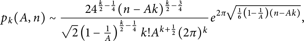
 $$ \begin{align} &p_{\leq k}(A;n)\sim \frac{24^{\frac k2-\frac14}n^{\frac k2-\frac34}}{\sqrt2\left(1-\frac1A\right)^{\frac k2-\frac14}k!A^{k+\frac12}(2\pi)^k}e^{2\pi\sqrt{\frac1{6}\left(1-\frac1A\right)n}},\nonumber\\[4pt] &p_{k}(A;n)\sim \frac{24^{\frac k2-\frac14}(n-Ak)^{\frac k2-\frac34}}{\sqrt2\left(1-\frac1A\right)^{\frac k2-\frac14}k!A^{k+\frac12}(2\pi)^k}e^{2\pi\sqrt{\frac1{6}\left(1-\frac1A\right)(n-Ak)}}. \end{align} $$
Example Here, we illustrate the convergence of the asymptotic for $p_{1}(3;n).$
Theorem 1.3(3) gives
$p_{1}(3;n).$
Theorem 1.3(3) gives
 $$ \begin{align*} p_{1}(3;n)\sim \frac{1}{6\pi(n-3)^{\frac14}}e^{\frac{2\pi\sqrt{n-3}}{3}}. \end{align*} $$
For convenience, we let $p^{*}_{1}(3;n)$
denote the right-hand side of this asymptotic. Table 1 illustrates the convergence of the asymptotic.
$p^{*}_{1}(3;n)$
denote the right-hand side of this asymptotic. Table 1 illustrates the convergence of the asymptotic.
Table 1 Asymptotics for $p_{1}(3;n)$

This paper is organized as follows. In Section 2, we prove Theorem 1.2, the generalization of the classical limiting distribution (1.5) of Erdös and Lehner. In Section 3, we recall the work of Buryak, Feigin, and Nakajima [Reference Buryak and Feigin2, Reference Buryak, Feigin and Nakajima3], which gives the infinite product generating functions for the Poincaré polynomials $P\left (X^{[n]}_{\alpha ,\beta };T\right )\!.$
These generating functions relate the Betti numbers to the partition functions
$P\left (X^{[n]}_{\alpha ,\beta };T\right )\!.$
These generating functions relate the Betti numbers to the partition functions $p_{\leq k}(\cdot ).$
We use these facts, combined with Theorem 1.2, to obtain Theorem 1.1. Finally, in Section 4, we obtain Theorem 1.3, the asymptotic formulas for the
$p_{\leq k}(\cdot ).$
We use these facts, combined with Theorem 1.2, to obtain Theorem 1.1. Finally, in Section 4, we obtain Theorem 1.3, the asymptotic formulas for the $p_{\leq k}(A;n)$
and
$p_{\leq k}(A;n)$
and $p_{k}(A;n)$
partition functions. These asymptotics follow from an application of Ingham’s Tauberian theorem.
$p_{k}(A;n)$
partition functions. These asymptotics follow from an application of Ingham’s Tauberian theorem.
2 Generalization of a theorem of Erdös and Lehner
Here, we prove Theorem 1.2. To prove the theorem, we combine some elementary observations about integer partitions with a delicate asymptotic analysis.
2.1 Elementary considerations
First, we begin with an elementary convolution involving the partition functions $p_{\leq k}(A;\cdot )$
,
$p_{\leq k}(A;\cdot )$
, $p_{\leq k}(\cdot ),$
and
$p_{\leq k}(\cdot ),$
and $p_{\mathrm {reg}}(A;n)$
, the number of
$p_{\mathrm {reg}}(A;n)$
, the number of $A$
-regular partitions of size
$A$
-regular partitions of size $n.$
Recall that a partition is
$n.$
Recall that a partition is $A$
-regular if all of its parts are not multiples of
$A$
-regular if all of its parts are not multiples of $A$
.
$A$
.
Proposition 2.1 If $A\geq 2$
is a positive integer, then for every positive integer
$A\geq 2$
is a positive integer, then for every positive integer $n$
, we have
$n$
, we have
 $$ \begin{align*} p_{\leq k}(A;n)=\sum_{j=0}^{\lfloor \frac{n}{A}\rfloor} p_{\leq k}(j)\cdot p_{\mathrm{reg}}(A; n-Aj). \end{align*} $$
Proof Every partition of $n$
with at most
$n$
with at most $k$
parts that are multiples of
$k$
parts that are multiples of $A$
can be represented as the direct product of an
$A$
can be represented as the direct product of an $A$
-regular partition and a partition into at most
$A$
-regular partition and a partition into at most $k$
parts that are all multiples of
$k$
parts that are all multiples of $A$
. If the sum of these multiples of
$A$
. If the sum of these multiples of $A$
is
$A$
is $Aj$
, then the
$Aj$
, then the $A$
-regular partition has size
$A$
-regular partition has size $n-Aj$
. Moreover, by dividing by
$n-Aj$
. Moreover, by dividing by $A$
, the multiples of
$A$
, the multiples of $A$
are represented by a partition of
$A$
are represented by a partition of $j$
into at most
$j$
into at most $k$
parts. This proves the claimed convolution.▪
$k$
parts. This proves the claimed convolution.▪
We also require an elegant inclusion–exclusion formula due to Erdös and Lehner [Reference Erdős and Lehner4] for $p_{\leq k}(n).$
Proposition 2.2 If $k$
and
$k$
and $j$
are positive integers, then
$j$
are positive integers, then
 $$ \begin{align*} p_{\leq k}(j)=\sum_{m=0}^{\infty} (-1)^{m} S_{k}(m;j), \end{align*} $$
whereFootnote 4
 $$ \begin{align} S_{k}(m;j):=\sum_{\substack{1\leq r_{1}<r_{2}<\dots <r_{m}\\ T_{m}\leq r_{1}+r_{2}+\dots+r_{m}\leq j-mk}} p\left(j-\sum_{i=1}^{m} (k+r_{i})\right) \end{align} $$
and $T_{m}:=m(m+1)/2.$
Proof By definition, $p_{\leq k}(j)$
is the number of partitions of
$p_{\leq k}(j)$
is the number of partitions of $j$
with at most
$j$
with at most $k$
parts. By considering conjugates of partitions, one can equivalently define
$k$
parts. By considering conjugates of partitions, one can equivalently define $p_{\leq k}(j)$
as the number of partitions of
$p_{\leq k}(j)$
as the number of partitions of $j$
with no parts
$j$
with no parts $\geq k+1$
. Since the number of partitions of size
$\geq k+1$
. Since the number of partitions of size $j$
that contain a part of size
$j$
that contain a part of size $k+r,$
where
$k+r,$
where $r\geq 1$
, equals
$r\geq 1$
, equals $p(j-(k+r)),$
we find that
$p(j-(k+r)),$
we find that $S_{k}(1,j)$
is generally an overcount for the number of partitions of
$S_{k}(1,j)$
is generally an overcount for the number of partitions of $j$
with at least one part
$j$
with at least one part $\geq k+1.$
Due to this overcounting, we find that
$\geq k+1.$
Due to this overcounting, we find that
 $$ \begin{align*} p(j)-S_{k}(1;j)\leq p_{\leq k}(j) \leq p(j)-S_{k}(1;j)+S_{k}(2;j), \end{align*} $$
which is obtained by taking into account those partitions which have at least two parts of distinct size $\geq k+1.$
The claim follows in this way by inclusion–exclusion.▪
$\geq k+1.$
The claim follows in this way by inclusion–exclusion.▪
2.2 Proof of Theorem 1.2
To prove Theorem 1.2, we require Propositions 2.1 and 2.2, and the asymptotics for $p_{\mathrm {reg}}(A;n).$
Thanks to the identity
$p_{\mathrm {reg}}(A;n).$
Thanks to the identity
 $$ \begin{align*} \prod_{n=1}^{\infty}(1+q^{n}+q^{2n}+\dots + q^{(A-1)n}) =\prod_{n=1}^{\infty}\frac{(1-q^{An})}{(1-q^{n})}= \sum_{n=0}^{\infty} p_{\mathrm{reg}}(A;n)q^{n}, \end{align*} $$
we find that $p_{\mathrm {reg}}(A;n)$
equals the number of partitions of
$p_{\mathrm {reg}}(A;n)$
equals the number of partitions of $n$
where no part occurs more than
$n$
where no part occurs more than $A-1$
times. Hagis [Reference Hagis10] obtained asymptotics for the number of partitions where no part is repeated more than t times, and letting
$A-1$
times. Hagis [Reference Hagis10] obtained asymptotics for the number of partitions where no part is repeated more than t times, and letting $t=A-1$
in Corollary 4.2 of [Reference Hagis10] gives the following theorem.
$t=A-1$
in Corollary 4.2 of [Reference Hagis10] gives the following theorem.
Theorem 2.3 If $A\geq 2,$
then we have
$A\geq 2,$
then we have
 $$ \begin{align*} p_{\mathrm{reg}}(A;n)=C_{A} (24n-1+A)^{-\frac{3}{4}}\exp\left(C\sqrt{\frac{A-1}{A}\left(n+\frac{A-1}{24}\right)}\right) \left(1+O(n^{-\frac{1}{2}})\right)\!, \end{align*} $$
where $C:=\pi \sqrt {2/3}$
and
$C:=\pi \sqrt {2/3}$
and $C_{A}:=\sqrt {12}A^{-\frac {3}{4}}(A-1)^{\frac {1}{4}},$
and the implied constant is independent of
$C_{A}:=\sqrt {12}A^{-\frac {3}{4}}(A-1)^{\frac {1}{4}},$
and the implied constant is independent of $A$
.
$A$
.
Proof of Theorem 1.2
Thanks to Propositions 2.1 and 2.2, we have that
 $$ \begin{align} \frac{p_{\leq k}(A;n)}{p(n)} =\sum_{j=0}^{\lfloor \frac{n}{A}\rfloor} \frac{\left(\sum_{m=0}^{\infty} (-1)^{m} S_{k}(m;j)\right) p_{\mathrm{reg}}(A;n-Aj)}{p(n)}. \end{align} $$
The proof follows directly from this expression by a sequence of observations involving the asymptotics for $p(\cdot )$
and
$p(\cdot )$
and $p_{\mathrm {reg}}(A;\cdot ),$
combined with the earlier work of Erdös and Lehner on the sums
$p_{\mathrm {reg}}(A;\cdot ),$
combined with the earlier work of Erdös and Lehner on the sums $S_{k}(m;j).$
Thanks to the special choice of
$S_{k}(m;j).$
Thanks to the special choice of $k_{n}=k_{n}(x)$
, this expression yields the Taylor expansion of the claimed cumulative Gumbel distribution in
$k_{n}=k_{n}(x)$
, this expression yields the Taylor expansion of the claimed cumulative Gumbel distribution in $x,$
as
$x,$
as $n\rightarrow +\infty .$
In other words, these asymptotics conspire so that the dependence on
$n\rightarrow +\infty .$
In other words, these asymptotics conspire so that the dependence on $n$
vanishes in the limit.
$n$
vanishes in the limit.
For convenience, we let $S^{*}_{k}(m;j):=S_{k}(m;j)/p(j).$
In terms of
$S^{*}_{k}(m;j):=S_{k}(m;j)/p(j).$
In terms of $S^{*}_{k}(m,j),$
(2.2) becomes
$S^{*}_{k}(m,j),$
(2.2) becomes
 $$ \begin{align} \frac{p_{\leq k}(A;n)}{p(n)} =\sum_{j=0}^{\lfloor \frac{n}{A}\rfloor} \frac{\left(\sum_{m=0}^{\infty} (-1)^{m} S^{*}_{k}(m;j)\right) p(j)p_{\mathrm{reg}}(A;n-Aj)}{p(n)}. \end{align} $$
To make use of this formula, we begin by employing the method of Erdös and Lehner mutatis mutandis, which we briefly recapitulate here. For $k\rightarrow +\infty ,$
with
$k\rightarrow +\infty ,$
with $j$
and m fixed, Erdös and Lehner proved (see (2.5) of [Reference Erdős and Lehner4]) that
$j$
and m fixed, Erdös and Lehner proved (see (2.5) of [Reference Erdős and Lehner4]) that
 $$ \begin{align} S^{*}_{k}(m;j) =\frac{1}{m!}\left(\frac{2}{C}\sqrt{j} \exp\left(-\frac{C}{ 2\sqrt{j}}k \right)\right)^{m} +o_{j,m}(1). \end{align} $$
For every positive integer $m,$
this effectively gives
$m,$
this effectively gives
 $$ \begin{align*} S^{*}_{k}(m;j)=\frac{1}{m!}\cdot S^{*}_{k}(1;j)^{m} + o_{j,m}(1)\sim \frac{1}{m!}\cdot S_{k}^{*}(1;j)^{m}, \end{align*} $$
which Erdös and Lehner show produces, as functions in $x$
, the asymptotic
$x$
, the asymptotic
 $$ \begin{align} \sum_{m=0}^{\infty} (-1)^{m} S^{*}_{k_{n}}(m;j) =\exp(-S^{*}_{k_{n}}(1;j))\left(1+ o_{n}(1)\right)\!. \end{align} $$
We recall the choice of $k=k_{A,n}=k_{A,n}(x)=\frac {1}{AC} \sqrt {n} \log (n) +x \sqrt {n}.$
This is the exponential which arises in the exponential of the claimed cumulative distribution.
$k=k_{A,n}=k_{A,n}(x)=\frac {1}{AC} \sqrt {n} \log (n) +x \sqrt {n}.$
This is the exponential which arises in the exponential of the claimed cumulative distribution.
To make use of (2.5), it is convenient to recenter the sum on $j$
in (2.3) by setting
$j$
in (2.3) by setting $j=\frac {n}{A^{2}} +y.$
As (2.5) only involves
$j=\frac {n}{A^{2}} +y.$
As (2.5) only involves $S^{*}_{k_{n}}(1;j),$
it suffices to note that when
$S^{*}_{k_{n}}(1;j),$
it suffices to note that when $m=1,$
(2.4) becomes
$m=1,$
(2.4) becomes
 $$ \begin{align} \kern25pt S^{*}_{{\color{black}k_{A,n}}}(1;j) &=\frac{2}{AC}\sqrt{n+A^{2}y}\cdot \exp\left(-\frac{\log(n)}{ 2\sqrt{1+yA^{2}/n}} -\frac{xAC}{ 2\sqrt{1+yA^{2}/n}} \right) +o_{n}(1). \end{align} $$
As the proof relies on (2.3), we must also estimate the quotients
 $$ \begin{align*} \frac{p(j)p_{\mathrm{reg}}(A;n-Aj)}{p(n)}. \end{align*} $$
Thanks to the Hardy–Ramanujan asymptotic for $p(n)$
and Theorem 2.3, we have
$p(n)$
and Theorem 2.3, we have
 $$ \begin{align} &\nonumber\frac{p(j)p_{\mathrm{reg}}(A;n-Aj)}{p(n)}\\ & =\frac{C_{A}}{(24n-24Aj-1+A)^{\frac{3}{4}}} \frac{n}{j}\exp{\left(C\left(\sqrt{j}-\sqrt{n}+\sqrt{\frac{A-1}{A}\left(n-Aj+\frac{A-1}{24}\right)}\right)\right)}\cdot\left(1+O_{j}(n^{-\frac{1}{2}})\right)\notag\\ & =\frac{C_{A}}{(24n-24n/A-24Ay-1+A)^{\frac{3}{4}}} \frac{A^{2}n}{n+A^{2}y}\notag\\ &\ \ \ \ \ \ \ \ \ \ \times \exp{\left(C\left(\sqrt{n/A^{2}+y}-\sqrt{n}+\sqrt{\frac{A-1}{A}\left(n-n/A-Ay+\frac{A-1}{24}\right)}\right)\right)} \cdot\left(1+O_{y }(n^{-\frac{1}{2}})\right)\!. \end{align} $$
The last manipulation uses the change of variable for $j$
.
$j$
.
We will make use of (2.5)–(2.7) to complete the proof. To this end, we let $j=\lfloor n/A^{2}\rfloor +y$
essentially as above, but now modifiedFootnote
5
so that the y are integers. We then rewrite (2.3) as
$j=\lfloor n/A^{2}\rfloor +y$
essentially as above, but now modifiedFootnote
5
so that the y are integers. We then rewrite (2.3) as
 $$ \begin{align*}\frac{p_{\leq {\color{black}k_{A,n}}}(A;n)}{p(n)} =\Sigma_{1}+\Sigma_{2}+\Sigma_{3}, \end{align*} $$
where $\Sigma _{1}$
is the sum over
$\Sigma _{1}$
is the sum over $-n/A^{2}\leq y< -n^{3/4}\log (n)$
,
$-n/A^{2}\leq y< -n^{3/4}\log (n)$
, $\Sigma _{2}$
is the sum over
$\Sigma _{2}$
is the sum over $-n^{3/4}\log (n)\leq y\leq n^{3/4}\log (n),$
and
$-n^{3/4}\log (n)\leq y\leq n^{3/4}\log (n),$
and $\Sigma _{3}$
is the sum over
$\Sigma _{3}$
is the sum over $n^{3/4}\log (n)\leq y\leq n(1/A-1/A^{2}).$
We shall show that the main contribution will come from
$n^{3/4}\log (n)\leq y\leq n(1/A-1/A^{2}).$
We shall show that the main contribution will come from $\Sigma _{2},$
and that
$\Sigma _{2},$
and that $\Sigma _{1}$
and
$\Sigma _{1}$
and $\Sigma _{3}$
vanish as
$\Sigma _{3}$
vanish as $n\rightarrow +\infty .$
To establish the vanishing of $\Sigma _{1}+\Sigma _{3},$
we consider the case that
$\Sigma _{1}+\Sigma _{3},$
we consider the case that $|y|> n^{3/4}\log (n).$
For such y, we have
$|y|> n^{3/4}\log (n).$
For such y, we have
 $$ \begin{align*} \sqrt{n/A^{2}+y}-\sqrt{n}+\sqrt{\frac{A-1}{A}\left(n-n/A-Ay+\frac{A-1}{24}\right)}= O_{y}(\sqrt{n}), \end{align*} $$
where the implied constant is negative. Moreover, (2.6) implies that $S^{*}_{{\color {black}k_{A,n}}} (1;n/A^{2}+y)=O(\sqrt {n}),$
where the implied constant is positive. Thus, for y in these ranges, both
$S^{*}_{{\color {black}k_{A,n}}} (1;n/A^{2}+y)=O(\sqrt {n}),$
where the implied constant is positive. Thus, for y in these ranges, both $\frac {p(j)}{p(n)} p_{\mathrm {reg}}(A;n-Aj)$
and
$\frac {p(j)}{p(n)} p_{\mathrm {reg}}(A;n-Aj)$
and $\sum _{m=0}^{\infty } (-1)^{m} S^{*}_{{\color {black}k_{A,n}}}(m;j)$
decay subexponentially, and so
$\sum _{m=0}^{\infty } (-1)^{m} S^{*}_{{\color {black}k_{A,n}}}(m;j)$
decay subexponentially, and so
 $$ \begin{align*}\lim_{n\to \infty} \Sigma_{1}+\Sigma_{3}=0.\end{align*} $$
We now consider $\Sigma _{2}$
, where
$\Sigma _{2}$
, where $|y|\leq n^{3/4}\log (n).$
In this range, (2.6) becomes
$|y|\leq n^{3/4}\log (n).$
In this range, (2.6) becomes
 $$ \begin{align} \qquad S^{*}_{{\color{black}k_{A,n}}}(1;j) &=\frac{2}{AC}\sqrt{n+A^{2}y}\cdot \exp\left(-\frac{\log(n)}{ 2\sqrt{1+yA^{2}/n}} -\frac{xAC}{ 2\sqrt{1+yA^{2}/n}} \right) +o_{n}(1) \end{align} $$
 $$ \begin{align} \hspace{-6.5pc} =\frac{2}{AC} \exp\left( -\frac 12 xAC \right) +o_{n}(1). \end{align} $$
Using (2.5), we obtain
 $$ \begin{align} \sum_{m=0}^{\infty} (-1)^{m} S^{*}_{{\color{black}k_{A,n}}}(m;j)=\exp\left (-\frac{2}{AC} \exp\left( -\frac 12 xAC \right)\right)\left(1+o_{n}(1)\right)\!. \end{align} $$
We now estimate (2.7) for these $|y|\leq n^{3/4}\log (n).$
Since we have
$|y|\leq n^{3/4}\log (n).$
Since we have
 $$ \begin{align*} &\sqrt{n/A^{2}+y}-\sqrt{n}+\sqrt{\frac{A-1}{A}\left(n-n/A-Ay+\frac{A-1}{24}\right)}\\ & \quad = -\frac{A^{4}}{8(A-1)}y^{2}n^{-3/2}+O_{A}(y^{3}n^{-5/2}), \end{align*} $$
the hypothesis on y allows us to turn (2.7) into
 $$ \begin{align*} \frac{p(j)p_{\mathrm{reg}}(A;n-Aj)}{p(n)} = \frac{A^{2} C_{A}}{(24n\frac{A-1}{A})^{3/4}}\times \exp{\left(-C\frac{A^{4}}{8(A-1)}\frac{y^{2}}{n^{3/2}} \right)} \cdot\left(1+O_{A }(n^{-\frac{1}{4}+\varepsilon})\right)\!. \end{align*} $$
Combined with (2.10), and using $C_{A}=\sqrt {12}A^{-\frac {3}{4}}(A-1)^{\frac {1}{4}},$
we obtain
$C_{A}=\sqrt {12}A^{-\frac {3}{4}}(A-1)^{\frac {1}{4}},$
we obtain
 $$ \begin{align} &\lim_{n\to\infty}\Sigma_2 =\lim_{n\to \infty }\sum_{|y|<n^{3/4}\log(n)} \frac{A^2}{96^{1/4}\sqrt{A-1}}\cdot \frac{1}{n^{3/4}}\nonumber\\ & \quad \cdot \exp\left (-\frac{CA^4}{8(A-1)}\frac{y^2}{n^{3/2}}-\frac{2}{AC} \exp\left( -\frac 12 xAC \right)\right) \cdot\left(1+o_{A }(1)\right)\!. \end{align} $$
Approximating the right-hand side as a Riemann sum, we obtain
 $$ \begin{align} \lim_{n\rightarrow +\infty} \Sigma_{2}=\lim_{n\rightarrow +\infty} \frac{A^{2}}{96^{1/4}\sqrt{A-1}}\int_{-\log(n)}^{\log(n)} \exp\left (-\frac{CA^{4}}{8(A-1)}t^{2}-\frac{2}{AC} \exp\left( -\frac 12 xAC \right)\right) dt, \end{align} $$
where $n$
only appears in the limits of integration. To obtain this, we have used the substitutions
$n$
only appears in the limits of integration. To obtain this, we have used the substitutions $t=yn^{-3/4}$
and
$t=yn^{-3/4}$
and $dt=n^{-3/4}dy,$
and employ the fact that the widths of the subintervals defining the Riemann sums tend to 0. Expanding as an integral over
$dt=n^{-3/4}dy,$
and employ the fact that the widths of the subintervals defining the Riemann sums tend to 0. Expanding as an integral over $\mathbb {R}$
, this expression simplifies to
$\mathbb {R}$
, this expression simplifies to
 $$ \begin{align*} \exp\left ( -\frac{2}{AC} \exp\left( -\frac 12 xAC \right)\right)\!. \end{align*} $$
Therefore, as a function in $x,$
we have
$x,$
we have
 $$ \begin{align*} \lim_{n\rightarrow +\infty}\frac{p_{\leq k_{A,n}}(A;n)}{p(n)}= \exp\left ( -\frac{2}{AC} \exp\left( -\frac 12 xAC \right)\right)\!. \end{align*} $$
This completes the proof of the theorem.▪
3 Application to the Hilbert schemes $X_{\alpha ,\beta }^{[n]}$

Here, we recall the relevant generating functions for the Poincaré polynomials of the Hilbert schemes that pertain to Theorem 1.1. For the various Hilbert schemes on $n$
points, Göttsche, Buryak, Feigin, and Nakajima [Reference Buryak and Feigin2, Reference Buryak, Feigin and Nakajima3, Reference Göttsche6, Reference Göttsche7] proved infinite product generating functions for these Poincaré polynomials. For Theorem 1.1, we require the following theorem.
$n$
points, Göttsche, Buryak, Feigin, and Nakajima [Reference Buryak and Feigin2, Reference Buryak, Feigin and Nakajima3, Reference Göttsche6, Reference Göttsche7] proved infinite product generating functions for these Poincaré polynomials. For Theorem 1.1, we require the following theorem.
Theorem 3.1 (Buryak and Feigin)
If $\alpha , \beta \in \mathbb {N}$
are relatively prime, then we have that
$\alpha , \beta \in \mathbb {N}$
are relatively prime, then we have that
 $$ \begin{align*} G_{\alpha,\beta}(T;q):=\sum_{n=0}^{\infty} P\left(X^{[n]}_{\alpha,\beta};T\right)q^{n}=\frac{(q^{\alpha+\beta};q^{\alpha+\beta})_{\infty}}{(q;q)_{\infty}(T^{2}q^{\alpha+\beta};q^{\alpha+\beta})_{\infty}}. \end{align*} $$
Remark The Poincaré polynomials in these cases only have even degree terms (i.e., odd index Betti numbers are zero). Moreover, letting $T=1$
in these generating functions give Euler’s generating function for
$T=1$
in these generating functions give Euler’s generating function for $p(n).$
Therefore, we directly see that
$p(n).$
Therefore, we directly see that
 $$ \begin{align*} p(n)=P\left(X^{[n]}_{\alpha,\beta};1\right)\!. \end{align*} $$
Of course, the proof of Theorem 3.1 begins with partitions of size $n$
.
$n$
.
Corollary 3.2 Assuming the notation and hypotheses above, if $d\mu ^{[n]}_{\alpha ,\beta }$
is the discrete measure for
$d\mu ^{[n]}_{\alpha ,\beta }$
is the discrete measure for $X^{[n]}_{\alpha ,\beta }$
, then
$X^{[n]}_{\alpha ,\beta }$
, then
 $$ \begin{align*} \Phi_{n}(\alpha, \beta; x)=\frac{1}{p(n)}\cdot \int_{-\infty}^{x} d\mu^{[n]}_{\alpha,\beta}= \frac{p_{\leq \frac{x}{2}}(\alpha+\beta;n)}{p(n)}. \end{align*} $$
Proof By Theorem 3.1, the Poincaré polynomial $P\left (X^{[n]}_{\alpha ,\beta };T\right )$
is the coefficient of
$P\left (X^{[n]}_{\alpha ,\beta };T\right )$
is the coefficient of $q^{n}$
of
$q^{n}$
of
 $$ \begin{align*} \frac{(q^{\alpha+\beta};q^{\alpha+\beta})_{\infty}}{(q;q)_{\infty}(T^{2}q^{\alpha+\beta};q^{\alpha+\beta})_{\infty}}. \end{align*} $$
Part (1) of Theorem 1.3 applied to $A=\alpha +\beta $
gives that the coefficient of
$A=\alpha +\beta $
gives that the coefficient of $T^{2k}$
in this expression is
$T^{2k}$
in this expression is $p_{k}(\alpha +\beta ;n)$
(the odd powers of T do not appear in this product as it is a function of
$p_{k}(\alpha +\beta ;n)$
(the odd powers of T do not appear in this product as it is a function of $T^{2}$
). Therefore, (1.3) becomes
$T^{2}$
). Therefore, (1.3) becomes
 $$ \begin{align*} P\left(X^{[n]}_{\alpha,\beta};T\right)=\sum_{j=0}^{\lfloor \frac{n}{\alpha+\beta}\rfloor} p_{j}(\alpha+\beta;n) T^{2j}= \sum_{j=0}^{2\lfloor \frac{n}{\alpha+\beta}\rfloor} \dim \left(H_{j}\left(X^{[n]}_{\alpha,\beta},\mathbb{Q}\right)\right)T^{j}. \end{align*} $$
Thus, the sum of coefficients up to $x$
, divided by
$x$
, divided by $p(n)$
, is
$p(n)$
, is
 $$ \begin{align*} \frac{1}{p(n)}\cdot \sum_{j\leq x}b_{j}(\alpha,\beta; n)=\frac{1}{p(n)}\cdot \sum_{j\leq x/2}p_{j}(\alpha+\beta;n)=\frac{p_{\leq \frac{x}{2}}(\alpha+\beta; n)}{p(n)}. \end{align*} $$
This completes the proof.▪
Proof of Theorem 1.1
To prove Theorem 1.1, we remind the reader that Theorem 1.2 gives the cumulative asymptotic distribution function for $p_{\leq k}(A;n)$
when
$p_{\leq k}(A;n)$
when $A\geq 2.$
Corollary 3.2, with
$A\geq 2.$
Corollary 3.2, with $A=\alpha +\beta ,$
identifies this partition distribution with the Betti distribution for the
$A=\alpha +\beta ,$
identifies this partition distribution with the Betti distribution for the $n$
point Hilbert schemes cut out by the
$n$
point Hilbert schemes cut out by the $\alpha , \beta $
torus action. The theorem follows by combining these two results.▪
$\alpha , \beta $
torus action. The theorem follows by combining these two results.▪
4 Asymptotic formulae for the
$p_{k}(A;n)$
partition functions

Here, we prove Theorem 1.3. To this end, we make use of Ingham’s Tauberian theorem [Reference Ingham12]. We note that this theorem is misstated in a number of places in the literature. Condition (3) in the statement below is often omitted. The reader is referred to the discussion in [Reference Bringmann, Jennings-Shaffer and Mahlburg1]. Here, we use a special caseFootnote 6 of Theorem 1.1 of [Reference Bringmann, Jennings-Shaffer and Mahlburg1].
Theorem 4.1 (Ingham)
Let $f(q)=\sum _{n\geq 0}a(n)q^{n}$
be a holomorphic function in the unit disk
$f(q)=\sum _{n\geq 0}a(n)q^{n}$
be a holomorphic function in the unit disk $|q|<1$
satisfying the following conditions:
$|q|<1$
satisfying the following conditions:
(1) The sequence $\left \{a(n)\right \}_{n\geq 0}$
is positive and weakly monotonically increasing.
$\left \{a(n)\right \}_{n\geq 0}$
is positive and weakly monotonically increasing.
(2) There exist $c\in \mathbb {C}, d\in \mathbb {R},$
and
$c\in \mathbb {C}, d\in \mathbb {R},$
and $N>0,$
such that as
$N>0,$
such that as $t\rightarrow 0^{+}$
, we have
$t\rightarrow 0^{+}$
, we have
 $$ \begin{align*} f(e^{-t}) \sim \lambda\cdot t^{d}\cdot e^{\frac{N}{t}}. \end{align*} $$
(3) For any $\Delta>0$
, in the cone
$\Delta>0$
, in the cone $|y|\leq \Delta x$
with
$|y|\leq \Delta x$
with $x>0$
and
$x>0$
and $z=x+iy$
, we have, as
$z=x+iy$
, we have, as $z\rightarrow 0$
,
$z\rightarrow 0$
,
 $$ \begin{align*} f(e^{-z})\ll |z|^{d}\cdot e^{\frac{N}{|z|}}. \end{align*} $$
Then, as $n\rightarrow +\infty $
, we have
$n\rightarrow +\infty $
, we have
 $$ \begin{align*} a(n)\sim\frac{\lambda\cdot N^{\frac d2+\frac14}}{2\sqrt\pi \cdot n^{\frac d2+\frac34}}e^{2\sqrt{Nn}}. \end{align*} $$
Proof of Theorem 1.3
We prove the claims one by one.
(1) We begin by recalling the q-Pochhammer symbol
 $$ \begin{align*}(a; q)_{k}:=\displaystyle\prod_{n=0}^{k-1}(1 -aq^{n} ).\end{align*} $$
Clearly, we have
 $$ \begin{align*} \frac{(q^{A};q^{A})_{\infty}}{(q;q)_{\infty}}=\prod_{j=1}^{A-1}\frac1{(q^{j};q^{A})_{\infty}}, \end{align*} $$
which in turn gives
 $$ \begin{align*} \frac{(q^{A};q^{A})_{\infty}}{(q;q)_{\infty}(Tq^{A};q^{A})_{\infty}}=\prod_{n\not\equiv0\,\,(\textrm{mod}\,\,{A})}\frac1{1-q^{n}}\quad \times\prod_{n\equiv0\,\,(\textrm{mod}\,\,{A})}\frac{1}{1-Tq^{n}}. \end{align*} $$
Expanding each term as a geometric series, we find that the coefficient of $T^{k}$
collects those partitions which have
$T^{k}$
collects those partitions which have $k$
parts which are
$k$
parts which are $0\,\,(\text {mod}\,\,{A})$
.
$0\,\,(\text {mod}\,\,{A})$
.
(2) We make use of the q-binomial theorem, which asserts that
 $$ \begin{align*} \sum_{n\geq0}\frac{(a;q)_{n}}{(q;q)_{n}}z^{n}=\frac{(az;q)_{\infty}}{(z;q)_{\infty}}. \end{align*} $$
Hence, if we let $[T^{k}]$
denote the coefficient of
$[T^{k}]$
denote the coefficient of $T^{k}$
, this theorem allows us to conclude that
$T^{k}$
, this theorem allows us to conclude that
 $$ \begin{align*} \frac{(q^{A};q^{A})_{\infty}}{(q;q)_{\infty}}[T^{k}]\left(\frac{1}{(Tq^{A};q^{A})_{\infty}}\right)&=\frac{(q^{A};q^{A})_{\infty}}{(q;q)_{\infty}}[T^{k}]\left(\sum_{n\geq0}\frac{(Tq^{A})^{n}}{(q^{A};q^{A})_{n}}\right)\\ & =\frac{q^{Ak}(q^{A};q^{A})_{\infty}}{(q;q)_{\infty}(q^{A};q^{A})_{k}}. \end{align*} $$
Arguing as in the proof of (1), we find the claimed generating function identity
 $$ \begin{align} \frac{(q^{A};q^{A})_{\infty}}{(q;q)_{\infty}(q^{A};q^{A})_{k}}=\sum_{n\geq0}p_{\leq k}(A;n)q^{n}. \end{align} $$
These two q-series identities, combined with (1), imply that $p_{k}(A;n)= p_{\leq k}(A;n-Ak).$
(3) To establish the desired asymptotics, we apply Theorem 4.1 to (4.1), which is facilitated by the modularity of Dedekind’s eta-function
 $$ \begin{align*} \eta(\tau):=q^{\frac{1}{24}}(q;q)_{\infty}. \end{align*} $$
This function is well known to satisfy
 $$ \begin{align*} \eta\left(-\frac{1}{\tau}\right)=\sqrt{\frac{\tau}{i}}\eta(\tau). \end{align*} $$
As a consequence of this transformation and the q-expansion $\eta (\tau )=q^{\frac 1{24}}+O(q^{\frac {25}{24}})$
near
$\eta (\tau )=q^{\frac 1{24}}+O(q^{\frac {25}{24}})$
near $\tau =i\infty $
(see, for example, page 53 of [Reference Zagier, Cartier, Julia, Moussa and Vanhove14]), for
$\tau =i\infty $
(see, for example, page 53 of [Reference Zagier, Cartier, Julia, Moussa and Vanhove14]), for $q=e^{-t}$
,
$q=e^{-t}$
, $t\rightarrow 0^{+},$
we find that
$t\rightarrow 0^{+},$
we find that
 $$ \begin{align} \log\left(\frac1{(q;q)_{\infty}}\right)=\frac{\pi^{2}}{6t}-\frac12\log\left(\frac{2\pi}{t}\right)+O(t). \end{align} $$
Thus, letting $t\mapsto At$
and taking a difference yields
$t\mapsto At$
and taking a difference yields
 $$ \begin{align} \log\left(\frac{(q^{A};q^{A})_{\infty}}{(q;q)_{\infty}}\right)=\frac{\pi^{2}}{6t}\left(1-\frac1A\right)-\frac{\log(A)}{2}+O(t). \end{align} $$
This calculation gives the behavior in the radial limit as $t\rightarrow 0^{+}$
of the infinite Pochhammer symbols in (4.1).
$t\rightarrow 0^{+}$
of the infinite Pochhammer symbols in (4.1).
To satisfy condition (3) of Theorem 4.1, we also need to estimate the quotient on the left-hand side of (4.3) for the regions $|y|\leq \Delta x$
. This is given directly in Section 3.1 of [Reference Bringmann, Jennings-Shaffer and Mahlburg1]. Namely, they show that in these regions, one has
$|y|\leq \Delta x$
. This is given directly in Section 3.1 of [Reference Bringmann, Jennings-Shaffer and Mahlburg1]. Namely, they show that in these regions, one has
 $$ \begin{align*} \frac{1}{(e^{-z};e^{-z})_{\infty}}=\sqrt{\frac{z}{2\pi}}\cdot\ e^{\frac{\pi^{2}}{6z}}\left(1+O_{\Delta}\left(\left|e^{-\frac{4\pi^{2}}{z}}\right|\right)\right) \end{align*} $$
and
 $$ \begin{align*} e^{-\frac{1}{z}}\leq e^{-\frac{1}{(1+\Delta^{2})|z|}}. \end{align*} $$
Thus, we have
 $$ \begin{align} \frac{1}{(e^{-z};e^{-z})_{\infty}}=\sqrt{\frac{z}{2\pi}}\cdot\ e^{\frac{\pi^{2}}{6z}}\left(1+O_{\Delta}\left(e^{-\frac{4\pi^{2}}{(1+\Delta^{2})|z|}}\right)\right)\!. \end{align} $$
Changing variables to let $z\mapsto Az$
, we then find
$z\mapsto Az$
, we then find
 $$ \begin{align} \frac{(e^{-Az};e^{-Az})_{\infty}}{(e^{-z};e^{-z})_{\infty}}&=\sqrt A\cdot e^{-\frac{\pi^{2}}{6z}\left(1-\frac1A\right)}\cdot\frac{\left(1+O_{\Delta}\left(e^{-\frac{4\pi^{2}}{A(1+\Delta^{2})|z|}}\right)\right)}{\left(1+O_{\Delta}\left(e^{-\frac{4\pi^{2}}{(1+\Delta^{2})|z|}}\right)\right)}\nonumber\\ &=\sqrt A\cdot e^{-\frac{\pi^{2}}{6z}\left(1-\frac1A\right)}\left(1+O_{\Delta}\left(e^{-\frac{4\pi^{2}}{A(1+\Delta^{2})|z|}}\right)\right)\!. \end{align} $$
Now, we turn to estimating the remaining factor in (4.1), namely, $1/(q^{A};q^{A})_{k}$
. On the line
$1/(q^{A};q^{A})_{k}$
. On the line $t\rightarrow 0^{+}$
, an important result of Zhang (see Theorem 2 of [Reference Zhang15]) gives that for
$t\rightarrow 0^{+}$
, an important result of Zhang (see Theorem 2 of [Reference Zhang15]) gives that for $0<t\rightarrow 0$
and
$0<t\rightarrow 0$
and $w\in \mathbb {C}$
,
$w\in \mathbb {C}$
,
 $$ \begin{align*} (e^{-wt};e^{-t})_{\infty}\sim \frac{\sqrt{2\pi}}{\Gamma(w)}e^{-\frac{\pi^{2}}{6t}-\left(w-\frac12\right)\log(t)}. \end{align*} $$
Letting $w=k+1$
and combining with (4.2), we conclude that
$w=k+1$
and combining with (4.2), we conclude that
 $$ \begin{align*} \frac{1}{(q;q)_{k}}=\frac{(q^{k+1};q)_{\infty}}{(q;q)_{\infty}} \sim\frac{\sqrt 2\pi}{k!}e^{-\frac{\pi^{2}}{6\varepsilon}-(k+1/2)\log(t)+\frac{\pi^{2}}{6t}-\frac12\log(2\pi/t)}=\frac{t^{-k}}{k!}. \end{align*} $$
Letting $t\mapsto At$
, we have
$t\mapsto At$
, we have
 $$ \begin{align} \frac{1}{(q^{A};q^{A})_{k}}\sim\frac{1}{k!A^{k}}t^{-k}. \end{align} $$
Turning to estimate $1/(q^{A};q^{A})_{k}$
in the regions
$1/(q^{A};q^{A})_{k}$
in the regions $|y|\leq \Delta x$
, we use the same argument in the proof of Theorem 2 of [Reference Zhang15]. One merely modifies the proof by replacing
$|y|\leq \Delta x$
, we use the same argument in the proof of Theorem 2 of [Reference Zhang15]. One merely modifies the proof by replacing $x$
with
$x$
with $|z|$
in Zhang’s setting to obtain
$|z|$
in Zhang’s setting to obtain
 $$ \begin{align*} {(e^{-A(k+1)z};e^{-Az})_{\infty}}\ll\frac{\sqrt{2\pi}}{k!}e^{-\frac{\pi^{2}}{6|z|}-\left(k+1-\frac12\right)\log|z|}, \end{align*} $$
as $z\rightarrow 0.$
Moreover, by combining with (4.4), we have
$z\rightarrow 0.$
Moreover, by combining with (4.4), we have
 $$ \begin{align} \frac{1}{(e^{-Az};e^{-Az})_{k}}=\frac{(e^{-A(k+1)z};e^{-Az})_{\infty}}{(e^{-z};e^{-z})_{\infty}}\ll\frac{|z|^{-k}}{k!}. \end{align} $$
Then, multiplying (4.5) and (4.7), we find that
 $$ \begin{align} \frac{(e^{-Az};e^{-Az})_{\infty}}{(e^{-z};e^{-z})_{\infty}(e^{-Az};e^{-Az})_{k}}\ll \frac{\sqrt{A}}{k!}|z|^{-k}e^{\frac{\pi^{2}}{6|z|}\left(1-\frac{1}{A}\right)} , \end{align} $$
which shows that condition (3) of Theorem 4.1 is satisfied.
Multiplying (4.3) with (4.6), where $q:=e^{-t}$
, we obtain
$q:=e^{-t}$
, we obtain
 $$ \begin{align*} \frac{(q^{A};q^{A})_{\infty}}{(q;q)_{\infty}(q^{A};q^{A})_{k}}\sim \frac{1}{k!A^{k+\frac12}}t^{-k}e^{\frac{\pi^{2}}{6t}\left(1-\frac 1A\right)}. \end{align*} $$
Moreover, the coefficients $\frac {(q^{A};q^{A})_{\infty }}{(q;q)_{\infty }(q^{A};q^{A})_{k}}$
are clearly positive as they count partitions. They are weakly increasing as there is an easy injection from the set of partitions of
$\frac {(q^{A};q^{A})_{\infty }}{(q;q)_{\infty }(q^{A};q^{A})_{k}}$
are clearly positive as they count partitions. They are weakly increasing as there is an easy injection from the set of partitions of $n$
with at most
$n$
with at most $k$
parts which are multiples of
$k$
parts which are multiples of $A$
into the set of partitions of
$A$
into the set of partitions of $n+1$
which have at most
$n+1$
which have at most $k$
parts which are multiples of
$k$
parts which are multiples of $A$
; simply add
$A$
; simply add $1$
to the partition, which does not affect the number of multiples of
$1$
to the partition, which does not affect the number of multiples of $A$
among the parts.
$A$
among the parts.
We are thus in the situation of Theorem 4.1, where we interpret (4.8) with
 $$ \begin{align*} \lambda=\frac{1}{k!A^{k+\frac12}},\quad d=-k, \quad N=\frac{\pi^{2}}{6}\left(1-\frac1A\right)\!. \end{align*} $$
Plugging these into Theorem 4.1 gives the desired asymptotic for $p_{\leq k}(A;n).$
The asymptotics for
$p_{\leq k}(A;n).$
The asymptotics for $p_{k}(A;n)$
follows from the identity
$p_{k}(A;n)$
follows from the identity $p_{k}(A;n)=p_{\leq k}(A;n-Ak)$
obtained in (2).▪
$p_{k}(A;n)=p_{\leq k}(A;n-Ak)$
obtained in (2).▪
Acknowledgment
The authors thank Kathrin Bringmann for helpful comments on an earlier version of this paper, and for pointing out the corrected version of the statement of Ingham’s Tauberian theorem. The authors also thank Ole Warnaar for comments on an earlier version of this paper. Finally, the authors thank the referee for pointing out typographical errors in the original manuscript.


 Open access