


Introduction
Hydraulic fracturing technologically shocked the US energy economy in the 2000s, resulting in rapid oil and natural gas production increases – also known as the “fracking boom.” US domestic natural gas production levels had been relatively stagnant from the 1980s through the 2000s, until 2005, when gas production began growing, nearly doubling from 2005 through 2020.Footnote 1 Because of this increase, natural gas overtook coal in 2015 as the plurality energy source used to generate electricity in the US.Footnote 2 The fracking boom was such a big deal that former President Obama, who was supported by environmental groups, tried to take credit in 2018, saying, “suddenly America’s like the biggest oil producer and the biggest gas – that was me, people.”Footnote 3 Throughout the same period – the late 2000s through 2010s – public opinion and social movement activity supporting more aggressive climate policies intensified (e.g., Caniglia et al. Reference Caniglia, Brulle and Szasz2015; Roser-Renouf et al. Reference Roser-Renouf, Stenhouse, Rolfe-Redding, Maibach and Leiserowitz2015). And yet, the US federal and (most) state governments did not enact significant policies to mitigate planet-warming emissions (e.g., Bang Reference Bang2015), despite this increased political pressure and escalating certainty and alarm among climate scientists.Footnote 4
The literature on the political economy of climate and environment emphasizes that the entrenchment of fossil fuel extraction and consumption interests is the main driver behind why governments across the world have not enacted more emissions-mitigating policies (e.g., Colgan, Green, and Hale Reference Colgan, Green and Hale2021; Mildenberger Reference Mildenberger2020; Stokes Reference Stokes2020). However, quantitative, causally identified evidence falsifying these propositions is relatively thin (for one exception, see Cooper, Kim, and Urpelainen Reference Cooper, Kim and Urpelainen2018). In this paper, I aim to fill that gap, leveraging the exogenous nature of the distribution of shale underneath US states as a treatment variable, to examine the possible impacts of fossil fuel endowments on climate policies at the state government level in the US. The fracking boom is a potentially fruitful setting to study causal effects, given the relatively short period of time when fracking technology rapidly spread across certain subsections of the country, opening up new fossil fuel reserves that had previously been untapped (Deutch Reference Deutch2011).
There is a rich literature in the study of state politics that makes a strong case for state governments as critical actors in the formation of American climate policy (for a review, see, e.g., Konisky and Woods Reference Konisky, Woods, Gray, Hanson and Kousser2018). While scholars have occasionally entertained “race to the bottom” theories that expect state governments to compete for minimal environmental regulation, states have been found to sometimes implement regulations more stringent than the federal government (Potoski Reference Potoski2001). During President Barack Obama’s time in office, after climate legislation stalled in Congress, the primary attempt to use executive action to mitigate greenhouse gas emissions (via the Clean Power Plan) would have given state governments significant authority of how to specifically achieve regulatory targets (Konisky and Woods Reference Konisky and Woods.2016). Independently, state governments have created their own unique climate or environmental regulations – often in part due to lack of significant federal policy changes – in areas such as fossil fuel drilling (Davis Reference Davis2017), renewable electricity (Carley et al. Reference Carley, Davies, Spence and Zirogiannis.2018), carbon pricing (Rabe Reference Rabe2018), and clean water rules (Fowler and Birdsall Reference Fowler and Birdsall.2021), among others. The institutionally federalist US political system makes state governments critical to the American ability to mitigate emissions.Footnote 5
In this paper, I study two climate policies (as outcome variables) that state governments have exercised control over for decades: the level of electricity generated by renewable sources (sometimes called “Renewable Portfolio Standards”) and low-emission vehicle (LEV) policy adoption. While renewable electricity targets may be familiar to readers, the LEV policy may not be: When a state government adopts a LEV policy, the vehicles that are sold in the state must subsequently meet more stringent pollution regulations.Footnote 6 The increased stringency of both policies would mitigate greenhouse gas emissions (and associated pollutants).Footnote 7 Fossil fuel extraction companies are known to oppose more stringent climate policies across the board (e.g., Brulle Reference Brulle2018; Stokes Reference Stokes2020). Employing a difference-in-difference (“diff-in-diff”) research design, I show that fracking negatively impacted LEV adoption and more suggestive evidence that fracking negatively impacted renewable electricity mandates. The latter evidence is more suggestive given its lack of extensive pretreatment outcome data to verify the common trends assumption (which is necessary for diff-in-diff research designs). To summarize the findings in other words, having the ability extract oil and/or natural gas via fracking within their geographic boundaries caused state governments to be less likely to adopt climate policies (LEV and renewable electricity policy).
My findings in this paper contribute to the climate political economy literature that shows that fossil fuel interests are one major factor that prohibits governments from mitigating societal emissions (Colgan, Green, and Hale Reference Colgan, Green and Hale2021; Cooper, Kim, and Urpelainen Reference Cooper, Kim and Urpelainen2018; Hughes and Urpelainen Reference Hughes and Urpelainen2015; Mildenberger Reference Mildenberger2020; Stokes Reference Stokes2020). In this particular case, fracking for shale oil and gas has prohibited American state governments from passing more stringent climate policies. Very few existing studies have produced quantitative (causal inference) evidence that fossil fuel resources have exerted effects on policymaking institutions (Cooper, Kim, and Urpelainen Reference Cooper, Kim and Urpelainen2018 is an exception), so this paper adds novel evidence on this front. Further, the findings in this paper join a small body of American politics research that has demonstrated political impacts of the fracking boom (Bishop and Dudley Reference Bishop and Dudley2017; Cooper, Kim, and Urpelainen Reference Cooper, Kim and Urpelainen2018; DiSalvo and Li Reference DiSalvo and Li2020; Fedaseyeu, Gilje, and Strahan Reference Fedaseyeu, Gilje and Strahan2015; Mallinson Reference Mallinson2014; Sances and You Reference Sances and You2022). However, nearly all of those other studies focus on campaign contributions, election winners, or voter turnout; only one studies something close to policy outcomes – environmental ratings of federal legislators (Cooper, Kim, and Urpelainen Reference Cooper, Kim and Urpelainen2018). This paper is the first to show that the fracking boom impacted overall policy outcomes (at the state government level) in particular. In addition, I offer the unique contribution of an original measurement of LEV policy adoption per state–year – a newly measured variable that may prove useful for other scholars of climate politics and policy.
In the following sections, I first review relevant literature, laying out the theoretical cases for economic interests influencing climate politics and the empirical gaps that I fill. Then, I clarify this paper’s theory and describe my original empirical design, including the inferential steps necessary to interpret this observational data analysis as evidence of causal effects. Finally, I argue that research which aims to test the influence of “business” on policy should account for “structural power” mechanisms, as this paper’s treatment (fossil fuel extraction) can be plausibly conceived to encompass the structural power of (fossil fuel) business activity.
Climate political economy and the American states
There is general agreement in the literature on the political economy of climate and environmental issues that economic interests drive policy outcomes. Specifically, these economic interests are energy endowments and the corporate, labor, and consumer interests that follow from the endowments. Much of this climate PE work is theoretical and qualitative; only a small handful of publications use quantitative causal inference research designs to show effects on politics of fossil fuel endowments and/or extraction. Some have specifically studied the American fracking boom, but none have examined state-level political outcomes nor actual policy enactment by governments.
Some recent prominent publications exhibit the importance of fossil fuel interests as a primary driver of climate politics across the world. Colgan, Green, and Hale (Reference Colgan, Green and Hale2021) argue that domestic climate policy outcomes can be best characterized by battles between those who own assets that drive climate change (e.g., fossil fuels) and assets vulnerable to climate impacts. Mildenberger (Reference Mildenberger2020) argues that carbon-intensive businesses and even fossil fuel labor unions drive policy outcomes in many countries, including the USA, Australia, and some European countries. Stokes (Reference Stokes2020) traces how organized fossil fuel interests used various tactics to roll back renewable energy policies at the state level in the US (an effect that this analysis will show using diff-in-diff analysis) – in crucial states where those industries perceive future profits to be made from more fossil fuel extraction. Hughes and Urpelainen (Reference Hughes and Urpelainen2015) argue that domestic climate politics is generally shaped by energy-intensive sectors (and constrained to some degree by public sentiment). Cory, Lerner, and Osgood (Reference Cory, Lerner and Osgood2021) analyze lobbying data to show that companies in all sectors of the US economy lobbied against federal climate legislation in the US because of their interdependence on carbon-intensive supply chains. All of these books and papers theoretically argue and show some qualitative or descriptive evidence that fossil fuel interests play some role in preventing more aggressive climate policy enactment.
Other more recent work applies quantitative methods to show plausible causal effects of economic interests driving environmental policy outcomes. Cooper, Kim, and Urpelainen (Reference Cooper, Kim and Urpelainen2018), also studying some effects of the US fracking boom, employ a local regression discontinuity design to show that a congressional district’s exposure to shale (at least in the Pennsylvania area) seemed to cause its federal representative to be more likely to vote against all environmental policy after the fracking boom’s height. Another recent prominent (but non-climate) paper shows a similar political-economic finding: Dasgupta (Reference Dasgupta2020) shows that agricultural interests in certain irrigation technology seemed to cause those jurisdictions to vote for conservative economic policies in 20th century American politics. This emerging quantitative causal inference work shows how economic interests can affect elections and policymaking regarding environmental politics at the federal level, but this line of research is still rather thin, only federally focused, and has not studied specific policy outcomes.Footnote 8
To be sure, there are forces other than fossil fuel interests that scholars argue matter in determining climate policies. Various kinds of institutional arrangements are likely to structure political outcomes in different ways at all levels of government (Hughes and Urpelainen Reference Hughes and Urpelainen2015). Specific to American climate politics at the state level, the degree of unified Democratic state government control or advantage in Democratic partisan identification at the voter level may increase a state’s likelihood of an increasingly stringent climate policy (Trachtman Reference Trachtman2020). Public opinion on environmental policy – and particularly government environmental spending – seems to be represented somewhat by state elected leaders (e.g., Fowler Reference Fowler2016; Johnson, Brace, and Arceneaux Reference Johnson, Brace and Arceneaux2005). Organized interest group representation on the pro-climate side (i.e., in opposition to fossil fuel interests) in the form of social movement protest activity may also lead a state government to implement stricter climate policies and decrease overall emissions (Muñoz, Olzak, and Soule Reference Muñoz, Olzak and Soule2018).
Particular to the substantive study of the effects of the fracking boom on climate politics, there are a few other papers in addition to Cooper, Kim, and Urpelainen (Reference Cooper, Kim and Urpelainen2018). One study showed that shale gas extraction in congressional districts seems to cause Republicans to win national electoral races at a higher rate (Fedaseyeu, Gilje, and Strahan Reference Fedaseyeu, Gilje and Strahan2015). Similarly, fracking has appeared to increase campaign donations to Republican candidates (DiSalvo and Li Reference DiSalvo and Li2020; Sances and You Reference Sances and You2022) but decrease overall voter turnout (Sances and You Reference Sances and You2022). Using basic correlational methods, papers have (unsurprisingly) found evidence that state legislators who receive more campaign contributions from oil and gas companies are more likely to support pro-fracking policies (Bishop and Dudley Reference Bishop and Dudley2017; Mallinson Reference Mallinson2014). Overall, the fracking boom’s political effects have seemed to advantage US Republicans, electorally. But this niche research area can be pushed further in terms of its methodological rigor and its focus on policies as outcomes.
In summary, the comparative and US politics literatures agree that energy interests are one significant driver of climate policy outcomes. Regarding the US fracking boom in particular, there is some evidence that it helped Republicans win more elections, and it seemed to cause voting by members of Congress in the Pennsylvania–Ohio–West Virginia–New York shale region to cast more anti-environmental votes (Cooper, Kim, and Urpelainen Reference Cooper, Kim and Urpelainen2018). However, there is not any existing evidence that the fracking boom affected (A) specific policy outcomes, (B) outcomes systematically across the entire geographic US, or (C) state-level government policy. In this paper, I aim to fill all those gaps.
In this paper, I set out to test the theory that the fracking boom – the rapid increase in shale oil and/or gas extraction from a subset of US states – decreased the stringency of climate policy in the states that were “treated” by fracking. As I will further describe in the Research Design section, I measure the treatment as shale coverage underneath a state’s boundaries, which is more properly understood as the potential to frack. This measurement is advantageous because it is more exogenous to political outcomes than the actual extraction of gas or oil, which is endogenous to the preexisting level of regulation, itself shaped by a state’s prior political battles. Further, the potential to frack better captures the future profit incentives that may drive corporate political behavior.
I test the impact of fracking on two state climate policy outcomes. Therefore, the two distinct hypotheses are as follows. First, an increased fracking potential in a state caused a decrease in the chances of that state government to adopt the LEV policy (i.e., a regulation that mitigates the global warming impacts from passenger vehicles). Second, an increased fracking potential in a state caused that state government to decrease its mandated share of electricity generation to come from renewable (i.e., climate-friendly) energy sources. Both of these hypotheses follow from the climate political economy literature, which agrees that the economic incentives associated with incumbent energy industries cause carbon-intensive sectors to oppose stringent climate policies and take political actions to prevent climate policy enactment (e.g., Cory, Lerner, and Osgood Reference Cory, Lerner and Osgood2021; Stokes Reference Stokes2020).
One economic aspect inherent to the commodity of shale fossil fuels is worth mentioning. Oil or natural gas produced by fracking can be transported across state lines. Therefore, if a fracking company extracts natural gas from a given state, it can transport and sell it elsewhere. This means there is less of an incentive to exert political pressure over climate policy in the same state where a fuel is extracted – so there may be an attenuated (i.e., less substantively large) effect of fracking in policy on the states where extracted, if companies are able to sell their product across all states. To be sure, it is still less expensive for a company to produce and sell gas or oil in the same state – all else equal – so there is still some incentive for the entire industry or an individual company to influence policy in that state where the fuel is extracted. This theoretical understanding does not bias the research design. It should only make us expect that fracking’s effects on policy may not be as large as they might be, if the commodity could only be sold in the state where it was extracted.
My analysis in this paper does not directly test any potential causal mechanisms. I simply test whether fracking potential seemed to cause policy outcomes to change, not how it might do so. However, to improve the intuitive plausibility of the paper, it can help to imagine mechanisms through which this causal effect may be operating.
Overall, the fracking boom increased the current profits of fossil fuel companies and their incentive to benefit from more future extraction. One large category of mechanisms includes classic theories of direct, organized business influence on policy. With increased current and future profits, it is possible that these companies explicitly intended to influence policy by spending more money on lobbying (e.g., Hacker and Pierson Reference Hacker and Pierson2010), direct campaign contributions (e.g., Hall and Wayman Reference Hall and Wayman1990), or outside “dark” money (e.g., Gilens, Patterson, and Haines Reference Gilens, Patterson and Haines.2021). These ways of using “instrumental power” may alter the political calculations of elected legislators, replace existing legislators with those friendlier to business interests, persuade the public on an issue relevant to business, provide more policy expertise that affects the eventual makeup of implemented policy, or have other effects that increase the chances that policy aligns with the interests or preferences of organized business.
Another category of mechanisms captures more indirect effects of such an economic interest. It is possible that fossil fuel companies influenced public opinion on climate policy in various states (as they seemed to have done nationally; e.g., Oreskes and Conway Reference Oreskes and Conway2011). It may be that fossil fuel companies used their power to more subtly change what issues matter to their workers and voters in any state (e.g., Gaventa Reference Gaventa1982). It is possible that unorganized “structural power” may be at work: policymakers’ own political interests have become dependent on fossil fuel companies’ provision of jobs and tax-generating economic production, and that is why politicians may do what fracking companies want (e.g., Culpepper Reference Culpepper2015; Lindblom Reference Lindblom1977; Przeworski and Wallerstein Reference Przeworski and Wallerstein1988). Citizen interests are in part driven by their source of jobs and income, which, in this case, become somewhat in tension with more stringent climate policy. Overall, there are many possible mechanisms through which an increase in fossil fuel extraction may cause a decrease in the stringency of climate policy. My analysis in this paper does not distinguish between possible influence mechanisms.
Research design
The hypothesis I test in this paper is that fracking caused state climate policies to be less stringent than they otherwise would have been in the counterfactual absence of fracking. I employ a difference-in-difference (diff-in-diff, DiD, or D-i-D) research design, which relies on particular assumptions. In this section, I describe the measurements of treatment, outcome, and control variables, and I justify the relevant assumptions. Crucially, I also describe the original dataset that I introduce and employ in this paper: LEV policy adoption by state year.
Treatment: Distribution of shale deposits
The concept underlying the treatment variable is the fracking of shale oil or gas. However, the empirical analogue (i.e., the measured quantity) I employ in this paper is simply the distribution of a shale deposit, which is more accurately understood as the potential to frack. This measurement is more advantageous than actual gas or oil extraction data, since the shale distribution is plausibly exogenous to state political variables that are likely independent drivers of the relevant policy outcomes (to be discussed further in the Additional Assumption subsection). More specifically, the measurement of the treatment here is the share of any given state’s geography covered (underneath) by shale.Footnote 9 It may be more accurate to measure the treatment variable as the actual volume of shale oil or gas reserves (by geographic area), but these data do not appear to exist for shale reserves, specifically; fortunately, the same measurement I employ (i.e., two-dimensional area) was used by Cooper, Kim, and Urpelainen Reference Cooper, Kim and Urpelainen2018) in their study of causal impacts of fracking on congressional voting.Footnote 10 Here, I code treatment as shale distribution in multiple ways: greater than zero proportion of a state covered by shale (which includes 29 states), greater than 5% of a state (21 states), greater than 10% of a state (16 states), and greater than 20% of a state (10 states). I study 49 out of 50 states – Texas is dropped for inferential reasons (see footnote).Footnote 11 Since the estimation strategy is difference-in-difference, a unit’s status of being in the treated or untreated group takes on a binary value (0/1) for each of these possible treatment statuses.
The map in Figure 1 shows the distribution of shale reserves that are known to have natural gas or oil.

Figure 1. Geographic distribution of shale deposits in the US.
Source: Post Carbon Institute. https://shalebubble.org/dbd-map/.
The potential to frack (and actual fracking wells, also shown on the map) is distributed around multiple parts of the country – concentrated in a few regions but still affecting many states. Table 1 lists which groups of states fall into which treatment status categories.
Table 1. List of state groups by treatment status, by different level of treatment

I conservatively take the beginning of the treatment period to be 2004.Footnote 12 The actual extraction of shale oil and gas slowly increased through the mid-2000s, really picking up closer to 2010. Therefore, I employ multiple treatment period options: 2004–2006, 2004–2008, and 2004–2010.Footnote 13 2004–2006, the shortest treatment period, is most likely to avoid capturing other sorts of (time-variant) relevant political dynamics changing in states. Alternatively, 2004–2010 is most likely to pick up effects of a “stronger” treatment, since more shale oil and gas would have been extracted over that period, becoming more integral to a state’s political economy. Thus, I use multiple treatment time periods to estimate the relevant regression quantities.
Figure 2 shows the timing of shale gas extraction increases. The notable increase in shale gas extraction began around 2005–2006 and steadily increased. Extraction of oil from shale reserves similarly began in the mid-2000s and then steeply increased around 2010.Footnote 14 It would be ideal to be able to separate – by geography and time – the extraction of shale oil from shale gas in the data, as they are energy sources used in distinct sectors of the economy and are therefore of difference relevance to unique policies. In this paper’s case, LEV policy governs cars, which use mostly gasoline (from oil), and RPS policies govern electricity, which is powered by an array of sources (today by a far higher share of natural gas than oil; but in the early- and mid-2000s, a non-negligible share of US electricity came from petroleum/oil).Footnote 15 However, data limitations appear to make this impossible. I am forced to keep shale oil and gas bundled together as one treatment. Although some nuance is lost by keeping them bundled, it is nonetheless theoretically possible that any fossil fuel company (whether fracking for oil or gas) will oppose and fight any climate policy, whether it aims to mitigate emissions from automobiles (LEV) or electricity generation (RPS). Further, companies that extract oil also extract gas, so the political goals of oil and gas are often intertwined.Footnote 16 We therefore may not gain much unique treatment measurement by quantitatively separating oil from gas. Unfortunately, the data at hand cannot distinguish between these various theoretical possibilities.

Figure 2. Over-time increase in shale gas production in the USA.
Source: US Energy Information Administration, Annual Energy Outlook 2013 Early Release. https://www.eia.gov/outlooks/aeo/er/pdf/0383er(2013).pdf.
Outcome 1: Original data on LEV policy adoption
The first contribution I make in this paper is to introduce an originally collected dataset that reports which states adopted the LEV policy in which year – which is the first of two policy outcome variables I employ.Footnote 17 These LEV policy data take the form of state–year and spans 1991–2015, which encapsulates the beginning of the policy’s history in the states.Footnote 18
LEV is a policy that states have been able to adopt in order to decrease the air pollution and greenhouse gas impacts of vehicles sold in their state. However, most states do not have the legal ability to craft a LEV to their liking. California created LEV in 1990 – updating the policy over time to include different pollutants and increased levels – and all other states can only choose to adopt portions of California’s LEV; alternatively, they can default to federal vehicle emission standards. This legal regime exists because the Clean Air Act does not allow states to preempt federal regulations, except that California is specifically exempted from that rule (per section 209 of the Clean Air Act) because it took very early state action (in 1966) to mitigate pollution from vehicles.Footnote 19 Therefore, all states (other than California) face the policy choice between just two options: default to federal vehicle emission regulations or adopt California’s LEV. Therefore, the measurement of LEV adoption in this paper dichotomously only takes the value of 0 (non-adoption, defaulting to federal rules) or 1 (adopting California’s LEV).
The US federal government has had vehicle fuel standards in place since 1975, first for passenger cars and a few years later for “light trucks” (e.g., sport utility vehicles, pickup trucks). These regulations did not change much over a few decades (until the 2007 Energy Independence and Security Act). California, seeking to do more to mitigate the impact of vehicles on its air quality (and in later LEV iterations, the impact on the global climate), created the first LEV regulation in 1990, submitting a formal waiver to the federal government to allow the state to go above and beyond the federal rules.Footnote 20
This first LEV regulation affected vehicles in model years 1994–2003. It created maximum levels for many pollutants – including carbon monoxide, nitrogen oxide, and others – emitted from passenger cars, light-duty vehicles (e.g., minivans, SUVs), and medium-duty vehicles (e.g., box trucks, school buses). A full list of regulated pollutants is available in the source in the footnote. California then updated its LEV regulations in 1998 and 2004, increasingly the stringency of preexisting pollutant maxima and regulating new pollutants (e.g., carbon dioxide in its 2004 iteration). During this period of decades, the federal government did have some regulations governing similar pollutants, but California’s LEV policy was always more stringent.Footnote 21
Immediately after California adopted the first LEV iteration in 1990, other states began adopting LEV, as well (e.g., New York and Massachusetts in 1991 and Maine in 1993, even before the EPA formally approved California’s waiver in 1993), which was allowed under Section 177 of the Clean Air Act. Some state legislatures passed bills to adopt LEV (e.g., Connecticut and New Jersey in 2004) while some governors perceived they had the legal authority to adopt LEV via executive action, without legislation (e.g., Arizona in 2006, Delaware in 2010).Footnote 22 In total, original data collection yielded 15 total states (including California; see footnote) who have adopted LEV by 2015.Footnote 23 LEV adoption is coded as a binary outcome per state–year – 0 for non-adoption, 1 for adoption.Footnote 24
Outcome 2: Mandated renewable share of state electricity generation
The second outcome variable employed in this analysis is the share of a state’s electricity generation mix mandated to come from renewable sources. A higher share mandated to come from renewables is a more stringent climate policy, thus mitigating more greenhouse gas emissions. This is measured using data from the Lawrence Berkeley National Lab.Footnote 25 More precisely, it is total megawatt-hours (MWh) of electricity mandated to come from renewable sources, per state (and year), divided by total MWh generation per state (of all electricity sources),Footnote 26 to produce the percentage of renewable electricity mandated, per state and year. These renewable energy data include various definitions – decided by each individual state – of what counts as a “renewable” source (e.g., some states classify biomass as renewable). This variation in energy creates a bit of measurement error for this outcome variable. However, this should not create inferential problems: Even though the definition of “renewable” can vary, it does not appear to ever include natural gas, however classified, mitigating concerns that this outcome variable could also measure some of the treatment variable (i.e., fracking). Some combination of state legislatures and executive agencies has primary decision-making power over the level of renewable energy mandated. These outcome variable data are available for 1999–2017. Figure 3 shows the entire raw data to visually depict the variation over time for this variable (and labels for a few high- and low-percentage states).

Figure 3. For >0% shale coverage treatment status: raw data (entire y-axis shown).
Difference-in-difference assumption: Common trends
The primary assumption employed in diff-in-diff estimation is common trends – that the trend of the outcome variable for the treatment group would have continued, posttreatment, at the same trend that the control group’s observed outcomes did, in the absence of treatment. While this is an assumption and so cannot be seamlessly empirically verified, common trends charts (displaying the over-time trend in the outcome variable prior to treatment) can visually provide some increased level of confidence in this assumption. Figures 4 and 5 show common trends for the “strongest” two treatments (>20% and >10% shale coverage) for the first outcome variable, LEV adoption from 1991 to 2015 (the entire history of the data); common trends for other treatment types are shown in the Supplementary Material. (Note that the y-axis is cut down, as distinct from Figure 4, in these and some following charts, in order to visually center the group means.)
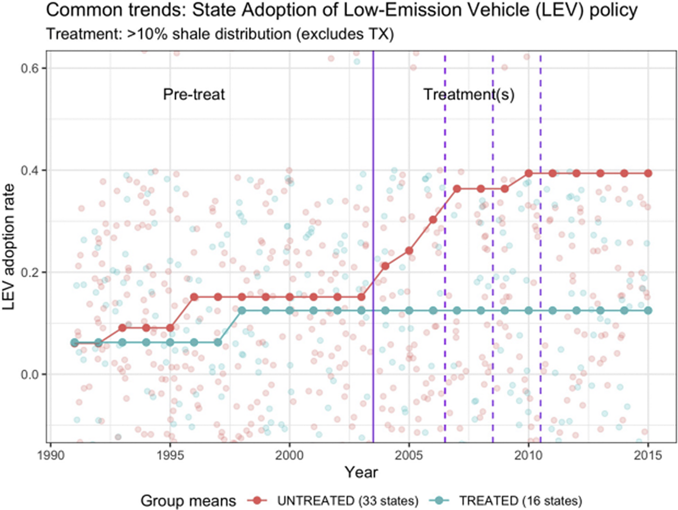
Figure 4. For >10% shale coverage treatment status: Common trends before, during, and after the height of the fracking boom.
Vertical lines (2003, 2013) indicate breaks between pretreatment (1999–2003), treatment (2004–2006, 2004–2008, or 2004–2010), and posttreatment (2007–2011, 2009–2013, or 2011–2015) periods. Raw data are plotted in the background of group means and trends. Multiple vertical dotted lines indicate the multiple treatment timing periods tested.
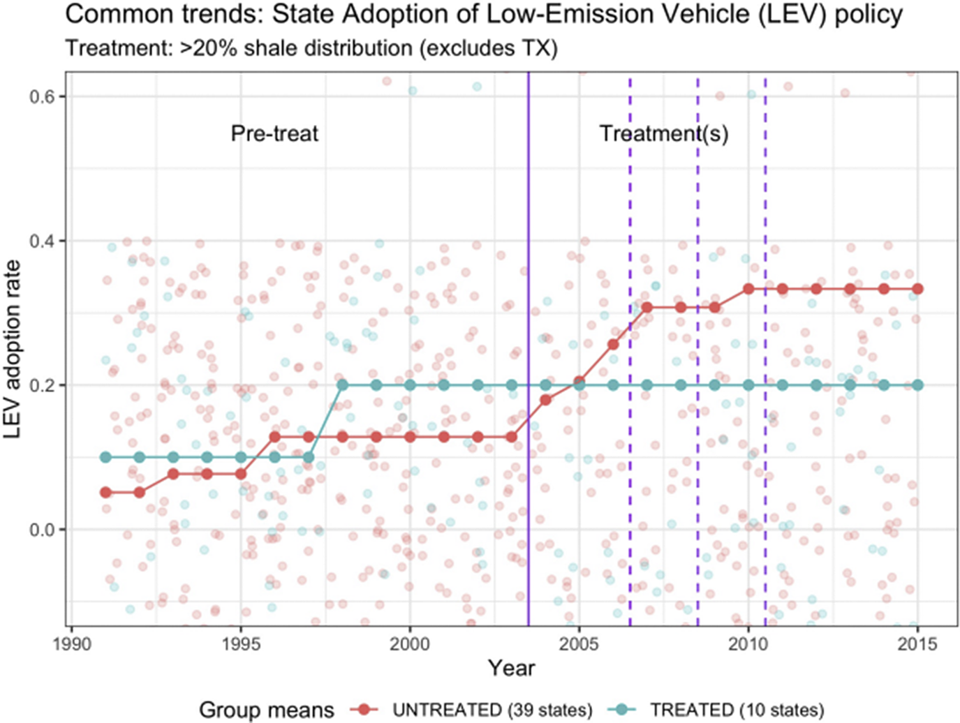
Figure 5. For >20% shale coverage treatment status: Vertical lines (2003, 2013) indicate breaks between pretreatment (1999–2003), treatment (2004–2006, 2004–2008, or 2004–2010), and posttreatment (2007–2010, 2009–2012, or 2011–2014) periods.
Figures 4 and 5 show that prior to the treatment period beginning (which is 2004; the vertical line sits at 2003.5), the levels of both treated and untreated groups moved at similar trends until the treatment period began, at which point, the untreated states (as a group) increased their LEV adoption rate. This common trend chart shows that the causal impact of fracking that plausibly happened was in fact one that caused treated states (those with shale) to not follow untreated states in increasing the adoption rate in the mid-late 2000s. I do not claim that the lack of fracking potential in untreated states is the proximate cause of their LEV adoption rate increase, but rather that fracking had a causal impact on holding back the group of treated states from an increased likelihood of adopting LEV.
Figure 6 plots the common trend for the second policy outcome variable, renewable electricity percentage mandates, for just one treatment status: >10% shale coverage (common trends for other treatment statuses are shown in the Supplementary Material). Since these policy data exist only starting in 1999, there are not much historical data to be able to see pretreatment common trends. Pretreatment, the treated and untreated states clearly diverge by small outcome variable percentages (<2% vs. 0%) in the trends of the outcome variable averages. Unfortunately, the lack of pretreatment data for this policy outcome variable (due to its recent development) leaves us with little ability to visually study these pretreatment common trends.

Figure 6. For >10% shale coverage treatment status: Vertical lines (2003, 2013) indicate breaks between pretreatment (1999–2003), treatment (2004–2006, 2004–2008, or 2004–2010), and posttreatment (2007–2010, 2009–2012, or 2011–2014) periods.
Additional assumption: Treatment exogeneity
The difference-in-difference research design does not rely on an exogenous treatment; it only relies on the assumption of common trends in the outcome variable. Overall, we want to be confident that the changed outcome of the treated group was truly caused by the treatment. However, employing the additional identifying assumption of exogeneity – that the geographic distribution of shale is orthogonal to political development prior to the fracking boom – strengthens our confidence that the diff-in-diff design is producing a causal effect. Cooper, Kim, and Urpelainen (Reference Cooper, Kim and Urpelainen2018), in employing shale geography as an exogenous treatment, write: “the definition of a shale play is ideally suited for an identification strategy based on the exogenous distribution…it does not require the onset of extraction activity or consider possible regulatory issues” (637).
If it is true that the assignment of shale to a state was exogenous, that means that no other variable relevant to this political context caused its observed variation. It is clear that shale was distributed by the geologic processes of the earth, which happened prior to the political development of each state. However, it is possible that the shale distribution could be correlated with similar resource development, like oil, which could affect a state’s political development. For that reason, regressions include one control variable that measures the prior decade of oil production (as a share of gross state product, or GSP).
A second way that the distribution of shale per state may be endogenous to renewable energy policies is if state policymakers – legislative or executive – knew about and anticipated the effect of fracking on a state’s politics. As previously discussed, fracking technology became widely available during the mid-2000s; before that, there was virtually zero shale oil or gas extraction. However, it also appears that there was little knowledge or political attention to fracking. Helpful qualitative research on the brief history of the fracking boom from Cooper, Kim, and Urpelainen (Reference Cooper, Kim and Urpelainen2018) supports this assertion. Cooper and coauthors read journalistic accounts and searched media headlines, finding little evidence of attention to potential shale gas drilling prior to the late 2000s outside of Texas: “[we] found no evidence of widespread interest in shale gas outside Texas by the end of 2004” (Cooper, Kim, and Urpelainen (Reference Cooper, Kim and Urpelainen2018, 638). Even though some states clearly knew they had shale basins underneath their geographic boundaries, estimates of how much gas could be extracted were quite low. Texas is dropped from this analysis.
Pretreatment control variables
Given the orthogonal causes of the geographic distribution of shale, we can have some confidence that the assignment of the treatment of shale for fracking is plausibly exogenous for this research design’s purposes. However, it is still not the case that shale distribution was assigned to states such that the treated and untreated groups are balanced by all imaginable relevant traits. The common trends assumption may be reasonable, but I still choose to employ control variables in the diff-in-diff regressions, to make the estimate of the effects of fracking more precise. This is similar logic to using pretreatment covariates in an experimental setting – to improve the precision of the treatment effect estimates, especially when the treated and untreated groups are not necessarily balanced by relevant covariates. It is also similar to using regression weights based on pretreatment covariates. In other words, we need to verify that it was not the case that states already (predisposed) likely to adopt less stringent climate policies were simply given shale. By different logic, the use of pretreatment covariates is also a hedge against the possibility that the common trends assumption seems less reasonable to some readers. Given the pretreatment common trends Figures 4 and 5, it appears far more valid for the LEV policy than for mandated renewables, given that pretreatment outcome data exist further back (historically) for LEV. However, in the Supplementary Material I display two-way fixed effects (i.e., state-time) regressions that do not use these pretreatment covariates; those regressions produce largely similar results.
In this paper’s primary regressions, I include a handful of covariates (i.e., control variables) that could plausibly drive differences in outcomes. One pair of control variables is unified Democratic state government control and gap in partisan affiliation of a state’s electorate (i.e., Democrats minus Republicans),Footnote 27 because a prior study (Trachtman Reference Trachtman2020) found that those both correlate quite well with a state adopting stringent renewable energy policy. This is intuitive, as it is generally understood in American politics that the Democratic Party coalition contains climate and environmental groups, while the Republican Party virtually does not. Crude oil extracted per stateFootnote 28 – divided by state GSPFootnote 29 – is also included as a covariate, as a measure of a state’s preexisting economic reliance on oil. State GSP (per capita) on its own is also included, in the chance that richer states have more leeway to adopt potentially costly climate policies. State government ideology is also included,Footnote 30 since more liberal state governments are more likely to adopt more stringent climate policy. Democratic governor is added as an additional control, since some state executive branches perceived they had the legal ability to adopt these policies without consent of the legislature.
A final key pretreatment covariate is a state population’s environmental policy opinion,Footnote 31 since the public’s opinion may certainly affect this policy outcome. The exact question wording is, “I support pollution standards even if it means shutting down some factories,” and answers range from 1 to 6 in levels of support. This is not a survey precisely about clean car or renewable electricity policy, but it may be a good enough proxy.Footnote 32 These rare state-level data are only available until 1998, so this variable is measured as the average of a state’s opinion from 1990 to 1998. Crucially, this control variable allows more weight to the claim that the evidence in this paper of the influence of fracking on policy change is contrary to this particular sense of the public interest – stated environmental policy preferences measured before the possibility of fracking.Footnote 33
Results
The following equation is the general form that all regressions employed for this research design use.
 $$ {\displaystyle \begin{array}{c}\mathrm{Policy}\hskip0.35em =\hskip0.35em {\beta}_0+\left({\beta}_1\mathrm{Treated}\right)+\left({\beta}_2\mathrm{Time}\right)+\left({\beta}_{3-i}\mathrm{Pre}\ \mathrm{Treatment}\ \mathrm{Controls}\right)\\ {}\hskip-18em +\left({\beta}_k\mathrm{Treated}\times \mathrm{Time}\right)+e\end{array}} $$
Therefore, $ \beta $
k estimates the causal effect of interest. The following table shows main diff-in-diff regression results for LEV policy, outcome 1, showing different treatment statuses (>0%, >5%, >10%, and > 20% shale coverage). Only the 2004–2006 treatment timing period is shown; the Supplementary Material shows similar tables for 2004–2008 and 2004–2010 treatment periods (results are very similar). In the Supplementary Material, I also display multiple two-way fixed effects models – that yield similarly significant results – to corroborate the main diff-in-diff results.
$ \beta $
k estimates the causal effect of interest. The following table shows main diff-in-diff regression results for LEV policy, outcome 1, showing different treatment statuses (>0%, >5%, >10%, and > 20% shale coverage). Only the 2004–2006 treatment timing period is shown; the Supplementary Material shows similar tables for 2004–2008 and 2004–2010 treatment periods (results are very similar). In the Supplementary Material, I also display multiple two-way fixed effects models – that yield similarly significant results – to corroborate the main diff-in-diff results.
Results in Table 2 show evidence of statistically significant correlations for the interaction term (i.e., treated × time), the relevant coefficient for diff-in-diff designs, for treatment statuses of >10% and >20% (but not >0% nor >5%). Results are displayed without pretreatment control variables results (full regression results tables shown in the Supplementary Material). This suggests that the possible causal effect of fracking potential on LEV policies in states operated at more significant levels of treatment (i.e., higher fracking share of a state). The statistically significant coefficients of −0.258 (>10% shale) and −0.216 (>20% shale) mean that being treated with fracking caused a 26 percentage point and 22 percentage point decrease, respectively, in the chances of adopting a LEV policy for the group of states. This is substantively large.
Table 2. Effect of fracking on LEV policy, 2004–2006 as treatment period.

Abbreviation: LEV, low-emission vehicle.
∗∗ p < 0.01;
∗ p < 0.05.
The following coefficient plot in Figure 7 shows the regression results (including all the treatment timing periods) in more visual terms.

Figure 7. Error bars show 95% confidence intervals.
State control variables are included in the regressions that produced these estimates.
Table 3 shows main diff-in-diff regression results for mandated renewable electricity, outcome 2, showing different treatment statuses (>0%, >5%, >10%, and > 20% shale coverage) for the 2004–2006 treatment timing period.
Table 3. Effect of fracking on renewable electricity policy, 2004–2006 as treatment period

∗∗ p < 0.01;
∗ p < 0.05.
Results in Table 3 show evidence of statistically significant correlations for the interaction term (i.e., treated × time), the relevant coefficient for diff-in-diff designs, for all treatment statuses of >5%, >10%, and >20% (but not >0%). This suggests that the possible causal effect of fracking potential on renewable electricity mandates in states operated at more significant levels of treatment, similar to the effects on LEV policy adoption. The statistically significant coefficients of −0.022, −0.024, and −0.022, respectively, mean that being treated with fracking caused a roughly 2 percentage points drop in mandated renewable portion of state electricity generation. This is a substantively meaningful coefficient size, as the average level of renewables mandated for the treated group (when treatment is measured as >10% shale, as in Figure 6) in 2015 is only 5% total. However, given the lack of pretreatment data to show some validation of the common trends assumption, we are left with only assuming no unobserved confounding for testing the effect of fracking on renewable electricity policy. Therefore, this evidence of fracking’s impact on state renewable electricity proportions is more suggestive than the LEV adoption evidence.
Unlike the LEV adoption (outcome 1) regression results, the analyses for fracking’s potential impact on mandated renewables (outcome 2) seem to increase as the treatment period lengthens. Therefore, Table 4 shows analyses for the 2004–2010 treatment period. Results for 2004–2008 treatment timing are shown in the Supplementary Material.
Table 4. Effect of fracking on renewable electricity policy, 2004–2010 as treatment period

∗∗p < 0.01;
∗p < 0.05.
The following coefficient plot in Figure 8 shows the regression results (including all the treatment timing periods) in more visual terms.

Figure 8. Error bars show 95% confidence intervals.
State control variables are included in the regressions that produced these estimates.
Placebo test results shown in the Supplementary Material – to test whether treatment may have affected the outcomes before 2004 – show null results.
While I have aimed to evaluate the influence of fracking on state climate policy, the shale oil and gas extraction happened at a particular moment in US political history. Therefore, it is worth noting some theoretical conditions that can help with hypothesizing about the generalizability of these findings. First, fracking happened decades and centuries after states had politically developed, so this influence happened at a particular point in the development of policy – there may have already been some level of entrenched influence in the policy prior the initial time period. Further, this influence under study is the potential effect of an economic interest in just one sector, and the independent variable is not often (for most states) the growth from zero fossil fuel corporation presence; instead, it is usually from some nonzero level of economic activity to a higher level. In these ways, these results estimate a “local” treatment effect in this paper – local in time, and local in the stage of fossil fuel development.
Is this evidence of business influence?
In this paper, I show some evidence that the fracking boom seemed to diminish climate policy stringency at the state level. Traditionally, “business influence” is usually thought to include lobbying, campaign spending, and occasionally attempts to sway public opinion. However, if we take seriously Lindblom’s (Reference Lindblom1977) argument that corporations may bias government policy in their favored direction via “structural power,” then we can conceive of this evidence of fracking’s influence on policy as the influence of business.
It is true that I do not test any hypotheses about which mechanisms may be at play, exerting the influence of fracking on policy. It could be traditional methods of organized business influence attempts, such as lobbying or campaign spending; it could be that more voters in the state saw their economic well-being as connected with the interests of fossil fuels and therefore opposed climate policy; it could be that fracking companies directly persuaded the public against climate policy through advertising campaigns; it may be that Lindblom’s (Reference Lindblom1977) “structural power” was at work, causing state legislators to see their political fortunes as interdependent with the jobs and tax revenue that the state fossil fuel industry was providing.
The point is that the production of a commodity seemed to bias government policy in a direction that favored that commodity’s future production. Under a more expansive definition of “business influence” – that Lindblom would argue for – I have uncovered evidence of the influence of business on policy. Therefore, future empirical attempts that aim to test hypotheses about business’ impact on politics and policy should ensure to account for multiple possible influence mechanisms (Hacker and Pierson Reference Hacker and Pierson2002). A subliterature in American politics sometimes argues that business may not actually influence policy all that much (e.g., Ansolabehere, De Figueiredo, and Snyder Reference Ansolabehere, De Figueiredo and Snyder2003; Fowler, Garro, and Spenkuch Reference Fowler, Garro and Spenkuch.2020; Smith Reference Smith2000), but those studies do not often account for some mechanisms that may, in fact, be at work.
Conclusion
The fracking boom generated enormous economic activity in some American states in the 2000s and 2010s. Contemporaneously, the climate crisis intensified – as did public opinion and social movement activity in support of more aggressive emissions-mitigating policies. While US emissions have begun falling, experts agree that far more stringent policies to further mitigate emissions will be necessary to stave off the worst effects of global warming.
In this paper, I have advanced our knowledge about the particular impact of fracking on politics and policy, showing that it harmed the ability for American state governments to enact emissions-mitigating policies. Specifically, the ability to extract shale oil or gas caused state governments to be less likely to enact the LEV policy and less likely to mandate a higher share of electricity generation to come from renewable energy. This research provides novel quantitative (causal inference) evidence that the fracking boom caused state-level climate policy outcomes to be less stringent than they otherwise would have been (in the absence of fracking). Existing studies have provided suggestive evidence that fracking has seemingly strengthened Republican political forces (DiSalvo and Li Reference DiSalvo and Li2020; Fedaseyeu, Gilje, and Strahan Reference Fedaseyeu, Gilje and Strahan2015; Sances and You Reference Sances and You2022) and has caused members of Congress to vote in more anti-environmental ways, across a host of issues (Cooper, Kim, and Urpelainen Reference Cooper, Kim and Urpelainen2018). Those papers provide initial looks at some effects of fracking, and I do not disagree with them. My argument in this paper goes deeper: I point to the influence of fossil fuel interests on the eventual prize of climate politics battles at the American subnational level, policies. To my knowledge, I add the (heretofore) only quantitative causal inference evidence of this. And after all, subnational governments (primarily states) are key to the US’s ability to mitigate the climate crisis overall, particularly in the face of federal government gridlock.
More broadly, my findings in this paper highlight the core assertion from political economy research: that economic resources are prominent drivers of policy outcomes. Other scholars have argued that fossil fuel interests – and their organized political strategies – have been primary drivers of climate politics (Colgan, Green, and Hale Reference Colgan, Green and Hale2021; Cooper, Kim, and Urpelainen Reference Cooper, Kim and Urpelainen2018; Hughes and Urpelainen Reference Hughes and Urpelainen2015; Mildenberger Reference Mildenberger2020; Stokes Reference Stokes2020). Together, my paper and this body of work imply that incumbent economic industries will be resistant to change, will likely fight in the organized political realm (as Oreskes and Conway Reference Oreskes and Conway2011; Stokes Reference Stokes2020 and others have shown in the organized battle of American climate politics), and may win policy battles more often than normative democratic theory portends. It is not public opinion or protest activity that primarily drives climate politics – concentrated economic interests dominate. This phenomenon may generalize from climate politics – not just federally, but also at the American state level – to other policy arenas for which large, profitable industries have a stake in the status quo economic regime: the regulation of finance, technology, healthcare, and many more. Policymakers and other powerful decision-makers should take note when an industry begins to carve out its share of the American economy – that industry may have also begin carving out its influence over public policy.
Lastly, I have conceptually argued that this paper’s evidence – of a commodity shock biasing policy in the direction of that commodity’s future economic well-being – should be considered evidence of the influence of business in politics. This conception of business influence takes the notion of “structural power” (Culpepper Reference Culpepper2015; Lindblom Reference Lindblom1977; Przeworski and Wallerstein Reference Przeworski and Wallerstein1988) seriously, that certain industrial sectors or individual corporations may have a deep hold over politicians by the nature that they can control jobs, consumer prices, and the raising of some tax revenue. Prior studies that have claimed to find little to no influence of money in politics. And while understanding specific influence mechanisms is outside the scope of this paper, my research design does account for all forms of instrumental and structural power influence. Therefore, future research would do well to theoretically imagine these more expansive pathways of influence and empirically test for mechanisms that include forms of structural power.
Supplementary Materials
To view supplementary material for this article, please visit http://doi.org/10.1017/spq.2022.17.
Data availability statement
Replication materials are available on SPPQ Dataverse at https://doi.org/10.15139/S3/UGCS7Y (Zacher Reference Zacher2022).
Acknowledgments
The author thanks Ian Turner for formally advising this paper in its initial stages, Jacob Hacker and Bryan Garsten for overseeing the course for which this paper was developed, and Jacob for comments throughout its various stages. Further, I appreciate other feedback on this project by participants at the American politics graduate student workshop and Research & Writing final presentation.
Funding statement
The author received general financial support for the research publication of this article from Yale University’s graduate program.
Conflict of interest
The authors declared no potential conflicts of interest with respect to the research, authorship, and/or publication of this article.
Author Biography
Sam Zacher is a PhD candidate at Yale University studying the politics of inequality, redistribution, and the climate crisis in contemporary America. His current research is aimed at understanding the nature of economic interests in the Democratic Party.


 Open access