


1. Introduction
The flow around a rotating sphere has drawn the attention of many researchers in recent years as it represents a canonical problem with many engineering and physics applications. For instance, such configuration may be found in multiple practical and natural phenomena like particle-driven flows (Shi & Rzehak Reference Shi and Rzehak2019), fluidized bed combustion (Liu & Prosperetti Reference Liu and Prosperetti2010; Feng & Musong Reference Feng and Musong2014), sports aerodynamics (Passmore et al. Reference Passmore, Tuplin, Spencer and Jones2008; Robinson & Robinson Reference Robinson and Robinson2013), seeds’ flight (Barois et al. Reference Barois, Huck, Paleo, Bourgoin and Volk2019; Rabault, Fauli & Carlson Reference Rabault, Fauli and Carlson2019) or free-falling/rising bodies (Ern et al. Reference Ern, Risso, Fabre and Magnaudet2012; Auguste & Magnaudet Reference Auguste and Magnaudet2018; Mathai et al. Reference Mathai, Zhu, Sun and Lohse2018), among others. In such applications, the instability of paths of the spherical bodies is shown to depend on the forces distributions acting on their surface and, therefore, on the flow regimes that are destabilized for different values of the Reynolds number and rotation rates. Consequently, a profound understanding of the physics of the flow around a rotating sphere and its instability features is required to predict the dynamics of rotating particles and evaluate possibilities of flow and path control.
The unstable flow regimes at the wake past a fixed sphere have been extensively characterized, as it represents a classical example of open flow leading to rich pattern formation and dynamical complexity. As reported by different numerical and stability analyses available in the literature, the flow experiences a complex sequence of laminar bifurcations as the Reynolds number  $\mbox { {Re}}$ increases (see, e.g. Sakamoto & Haniu Reference Sakamoto and Haniu1990; Johnson & Patel Reference Johnson and Patel1999; Fabre, Auguste & Magnaudet Reference Fabre, Auguste and Magnaudet2008; Fabre et al. Reference Fabre, Tchoufag, Citro, Giannetti and Luchini2017). For a static (non-rotating) sphere, the flow first experiences a steady bifurcation around $\mbox { {Re}}_{c1}\simeq 212$, leading to a steady, reflection-symmetric bifid wake (steady-state mode, Fabre et al. Reference Fabre, Auguste and Magnaudet2008), followed by a Hopf bifurcation at $\mbox { {Re}}_{c2}\simeq 272$ (Citro et al. Reference Citro, Siconolfi, Fabre, Giannetti and Luchini2017), leading to a periodic, vortex-shedding mode which preserves the axial reflection symmetry plane (RSP mode, Fabre et al. Reference Fabre, Auguste and Magnaudet2008). This reflection symmetry in the shedding process is lost around $\mbox { {Re}}_{c3}\simeq 375$, from which the wake starts to oscillate transversely (Chrust, Goujon-Durand & Wesfreid Reference Chrust, Goujon-Durand and Wesfreid2013).
When rotation is applied, the bifurcation scenario of the sphere wake is modified, generating even richer dynamics. In particular, as shown by Poon et al. (Reference Poon, Ooi, Giacobello and Cohen2010), the topology and frequency of the unstable flow regimes depend on the rotation rate  $\varOmega$ and the axis of rotation.
In general, the flow past streamwise rotating spheres has received considerably less attention than transversely rotating spheres (see, e.g. Citro et al. Reference Citro, Tchoufag, Fabre, Giannetti and Luchini2016), and their dynamics and controllability features are not yet fully understood. However, some numerical and experimental studies have focused on the flow topology and stability modifications produced in the sphere wake as the streamwise rotation speed increases (Kim & Choi Reference Kim and Choi2002; Niazmand & Renksizbulut Reference Niazmand and Renksizbulut2005; Skarysz et al. Reference Skarysz, Rokicki, Goujon-Durand and Wesfreid2018) at low values of Reynolds number. The problem can be also studied under linear stability analysis perspective as in Pier (Reference Pier2013) and Jiménez-González, Manglano-Villamarín & Coenen (Reference Jiménez-González, Manglano-Villamarín and Coenen2019). Moreover, the influence of streamwise rotation is not only restricted to the sphere, and it has been also studied in wakes behind other axisymmetric geometries which follow a similar series of bifurcations, as in Jiménez-González et al. (Reference Jiménez-González, Sanmiguel-Rojas, Sevilla and Martínez-Bazán2013) and Jiménez-González et al. (Reference Jiménez-González, Sevilla, Sanmiguel-Rojas and Martínez-Bazán2014) for blunt-based bodies.
The introduction of streamwise rotation introduces unsteadiness and asymmetry in the sphere wake. The steady state is substituted by a frozen rotation with azimuthal wavenumber  $m = -1$ symmetry (Kim & Choi Reference Kim and Choi2002; Jiménez-González et al. Reference Jiménez-González, Manglano-Villamarín and Coenen2019), the negative sign indicating that vortical structures wind in the direction opposite to the swirl motion. When either $Re$ or $\varOmega$ increase, the periodic behaviour of this low-frequency frozen state diverges to quasiperiodic or even chaotic states. The quasiperiodicity can be caused by the appearance of a medium-frequency component, related to the RSP mode of the non-rotating situation, or to the appearance of a component with $m=-2$ symmetry in the flow, for $Re<500$ and moderate $\varOmega$ values (Skarysz et al. Reference Skarysz, Rokicki, Goujon-Durand and Wesfreid2018; Lorite-Díez & Jiménez-González Reference Lorite-Díez and Jiménez-González2020). Moreover, in a more recent study, Lorite-Díez & Jiménez-González (Reference Lorite-Díez and Jiménez-González2020) also identified very complex patterns close to chaotic behaviours, by performing direct numerical simulations (DNS). More precisely, with the help of dynamic mode decomposition tools, the nonlinear regimes are reported to be characterized by three fundamental frequency components (related to unstable structures displaying $m=-1$, $m=-1$ and $m=-2$ symmetries, respectively) and their interactions. However, the time-stepping simulations do not provide a clear insight about the origin of instability of these complex regimes and the fundamental nature of the incommensurate or derived frequency components, so that the use of adjoint stability tools seem advisable to isolate fundamental modes and identify mechanisms of receptivity to forcing or control.
Additionally, the time-stepping simulations of such complex dynamical systems are generally demanding in terms of computational cost, especially close to bifurcations thresholds, where long convergence times are usually required to obtain statistically relevant solutions. As a matter of fact, alternative weakly nonlinear approaches, as those based on bifurcation theory (Golubitsky & Langford Reference Golubitsky and Langford1988), may be more efficient to elucidate the pattern of transitions and major features of flow regimes with increasing values of the problem parameters (i.e.  $\mbox { {Re}}$, $\varOmega$), by taking advantage of the symmetry of the base flow and proximity between successive instability thresholds. That said, the transition scenarios of complex systems with underlying symmetries usually lead to a large variety of pattern formations.
Close to the onset of stability, these patterns may be caused by a single instability, or alternatively, the system can display instabilities where several modes are concomitantly accountable for the destabilization of the trivial state. Besides, flow configurations controlled by a diversity of parameters may lose stability in diverse manners. A large diversity of patterns may emerge in the entire parameter space, and, in particular, one can find specific regions displaying mode competition. The combination of symmetry with a parameter space whose dimension is higher than one is a classical scenario where mode interaction occurs. The organizing centre of such cases is denoted as a bifurcation of codimension  $n$, with $n \in \mathbb {N}$. Codimension is herein loosely defined as the number of interacting modes, and also corresponds to the dimension of the low-order dynamical system model called the normal form capturing the essence of the dynamics. The interested reader can find more about pattern formation in symmetric systems in Golubitsky, Stewart & Schaeffer (Reference Golubitsky, Stewart and Schaeffer2012), while the study of the normal form of bifurcations with codimension higher than one may be found in the books of Guckenheimer (Reference Guckenheimer2010) or Kuznetsov (Reference Kuznetsov2013). The passage from a high-dimensional system to a reduced one with a slow manifold takes advantage of the theoretical framework provided by the singular perturbation theory. For example, the geometric singular perturbation theory, reviewed by Verhulst (Reference Verhulst2007), is a powerful technique within the singular perturbation theory. In the bifurcation theory of autonomous systems, it is customary to employ centre manifold or normal form reduction. This procedure has been employed for the study of bifurcations from steady states (Haragus & Iooss Reference Haragus and Iooss2010), maps (respectively Poincaré maps associated with a limit-cycle solution) (Kuznetsov & Meijer Reference Kuznetsov and Meijer2005), homoclinic and heteroclinic connections (Homburg & Sandstede Reference Homburg and Sandstede2010). The most commonly used computational procedures to determine the centre manifold are weakly nonlinear analysis, multiple scales expansion or the homological equation. In the past, these approaches have been exploited to study mode interaction in thermally driven convective motions, e.g. the Rayleigh–Bénard (Varé et al. Reference Varé, Nouar, Métivier and Bouteraa2020) and Langmuir circulation (Allen & Moroz Reference Allen and Moroz1997), in the fluid flow between counter-rotating cylinders, e.g. the Taylor–Couette flow (Golubitsky & Langford Reference Golubitsky and Langford1988) and its variants (Renardy et al. Reference Renardy, Renardy, Sureshkumar and Beris1996), in magnetoconvection (Rucklidge et al. Reference Rucklidge, Weiss, Brownjohn, Matthews and Proctor2000), in the flow past a rotating cylinder (Sierra et al. Reference Sierra, Fabre, Citro and Giannetti2020b) and in swirling jets (Meliga, Gallaire & Chomaz Reference Meliga, Gallaire and Chomaz2012).
In light of the aforementioned studies, for the parameters considered herein, one can expect that a linear stability analysis (LSA) discriminates at least three unsteady unstable fundamental modes: two with azimuthal wavenumber  $m=-1$ and a third one with $m=-2$; meaning that the organizing centre is a triple-Hopf bifurcation with $SO(2)$ symmetry. Despite the likely existence of three unstable modes, because the dimension of the parameter space is two, the triple-Hopf bifurcation is not expected to occur. Therefore, the approach followed herein for the study of the triple-Hopf bifurcation is based on the extension of the normal form obtained at codimension-two points to the codimension-three manifold. In practical terms, we determine a fifth-order truncation in terms of the expansion parameter of the normal form at codimension-two points, followed by a linear (respectively quadratic for linear coefficients) extension of normal form coefficients to a specific point in the parameter space. Such an approach is detailed in § 4 and it is similar to the centre-unstable manifold reduction, cf. Armbruster, Guckenheimer & Holmes (Reference Armbruster, Guckenheimer and Holmes1989), Podvigina (Reference Podvigina2006a), Podvigina (Reference Podvigina2006b) and Meliga, Chomaz & Sipp (Reference Meliga, Chomaz and Sipp2009a). In any case, once the normal form is determined, one can analyse the bifurcation scenario, which displays a rich variety of patterns, among which one can expect: rotating waves, quasiperiodic mixed modes or chaotic solutions displaying multiple frequency components, along with bi-stable states stemming from the coexistence of two stable rotating waves, mixed modes and rotating waves, diverse mixed modes or mixed modes and chaotic attractor.
Some of these transition features and bi-stable dynamics had been confirmed via time-stepping numerical simulations undertaken by Lorite-Díez & Jiménez-González (Reference Lorite-Díez and Jiménez-González2020) and Pier (Reference Pier2013) who reported a rich variety of spatio-temporal patterns. However, they did not perform an exhaustive analysis of the nature of the bifurcations between the distinct regimes. Therefore, the objective of the present research is twofold. The first objective is to undertake a global stability analysis to determine the connection between the observed patterns by Lorite-Díez & Jiménez-González (Reference Lorite-Díez and Jiménez-González2020) and the linear stability of helical modes. The identification of these fundamental modes allows an identification of the underlying physical mechanisms responsible for the instabilities and the receptivity of the flow to forcing or control possibilities. Secondly, the analysis of the normal form associated with the organizing centre serves to provide a complete phase portrait of the flow attractors before the emergence of temporal chaos and to unravel the transition towards chaotic spatio-temporal dynamics observed by Lorite-Díez & Jiménez-González (Reference Lorite-Díez and Jiménez-González2020) and Pier (Reference Pier2013).
The outline of the manuscript is as follows. First, the flow configuration and the numerical approach are presented in § 2. Second, we undergo a LSA in § 3, which identifies the most unstable global modes, their underlying physical mechanisms and sensitivity to forcing. Third, we introduce the methodology for the normal form reduction and we illustrate it with a bifurcation diagram at constant rotation rate in § 4. Then, in § 5 we pursue the study by comparing the normal form predictions with DNS results and we provide a complete phase diagram of the stable attractors of the flow in the range  $Re \leq 300$ and $\varOmega < 4$. Finally, in § 6 we summarise the main findings and we argue of some future applications of the study.
2. Methodology
2.1. Flow configuration – governing equations
The flow past an axisymmetric rotating body is controlled by two parameters: the Reynolds number ( $\mbox { {Re}}$) and the rotation rate ( ${{\varOmega }}$) which is defined as the ratio of the tangential velocity ${{\varOmega }^{\ast }}D^{*}/2$ on the sphere surface to the inflow velocity $W^{\ast }_\infty$. The fluid motion inside the domain is governed by the incompressible Navier–Stokes equations written in cylindrical coordinates $(r,\theta,z)$,
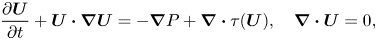 $$\begin{gather} \frac{\partial \boldsymbol{U}}{\partial t} + \boldsymbol{U}\boldsymbol{\cdot} \boldsymbol{\nabla}\boldsymbol{U} ={-}\boldsymbol{\nabla} P + \boldsymbol{\nabla} \boldsymbol{\cdot} \tau(\boldsymbol U ), \quad \boldsymbol{\nabla} \boldsymbol{\cdot} \boldsymbol U = 0, \end{gather}$$
 $$\begin{gather}\text{with } \tau(\boldsymbol{U}) = \frac{1}{\mbox{{Re}}} (\boldsymbol{\nabla} \boldsymbol U + \boldsymbol{\nabla} \boldsymbol U^{\rm T}), \quad \mbox{{Re}} = \frac{W^{{\ast}}_\infty D^{{\ast}}}{\nu^{{\ast}}}, \quad \varOmega = \frac{{{\varOmega}^{{\ast}}}D^{{\ast}}}{2 W^{{\ast}}_\infty}, \end{gather}$$
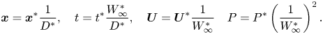 $$\begin{gather}\boldsymbol{x} = \boldsymbol{x}^{{\ast}} \frac{1}{D^{{\ast}}}, \quad t = t^{{\ast}} \frac{W^{{\ast}}_\infty}{D^{{\ast}}}, \quad \boldsymbol{U} = \boldsymbol{U}^{{\ast}} \frac{1}{W^{{\ast}}_\infty} \quad P = P^{{\ast}} \left(\frac{1}{W^{{\ast}}_\infty}\right)^{2}. \end{gather}$$
 Dimensional quantities are identified with the upperscript symbol  $^{\ast }$. Reference scales are specified in (2.1c). The dimensionless velocity vector $\boldsymbol {U} = (U,V,W)$ is composed of the radial, azimuthal and axial components, $P$ is the dimensionless reduced pressure and the viscous stress tensor, $\tau (\boldsymbol U )$. For representation purposes, it is sometimes necessary to use the Cartesian coordinates ( $x,y,z$), here $z$ denotes the streamwise direction, $y$ the vertical crosswise direction and $x$ the direction that forms a direct trihedral with $z$ and $y$. The incompressible Navier–Stokes equations (2.1) are complemented with the following boundary conditions:
 \begin{equation} \boldsymbol{U} = (0, \varOmega, 0) \text{ on } \varSigma_{b} \quad \boldsymbol{U} = (0, 0, 1) \text{ on } \varSigma_{i}. \end{equation}
No-slip boundary condition is set on the rotating sphere and a uniform boundary condition is set in the inlet, as shown in figure 1.
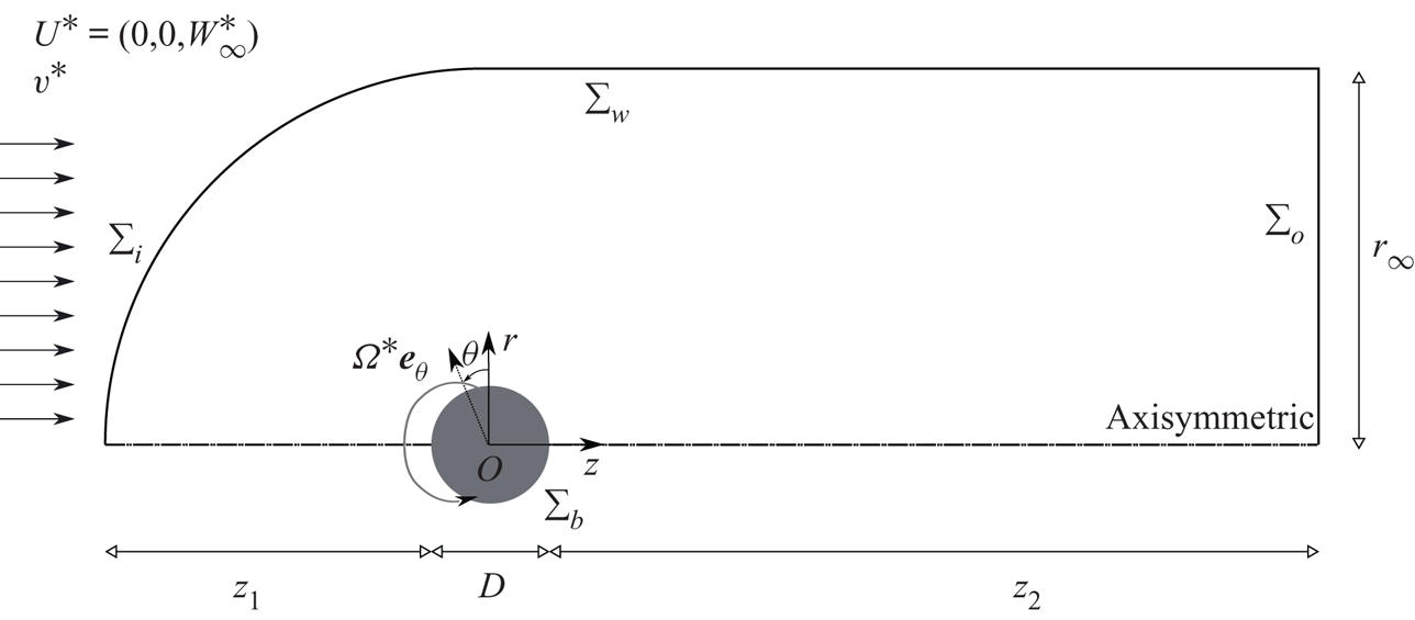
Figure 1. Sketch of the problem and geometric configuration.
In the sequel, Navier–Stokes equations (2.1) and the associated boundary conditions will be written symbolically under the form
 \begin{equation} \boldsymbol{B} \frac{\partial \boldsymbol{Q}}{\partial t} = \boldsymbol{F}(\boldsymbol{Q}, \boldsymbol{\eta}) \equiv \boldsymbol{L} \boldsymbol{Q} + \boldsymbol{N}(\boldsymbol{Q},\boldsymbol{Q}) + \boldsymbol{G} (\boldsymbol{Q},\boldsymbol{\eta}), \end{equation}
where  $\boldsymbol {B}$ is the projection matrix onto the velocity field with the flow state vector $\boldsymbol {Q} = [ \boldsymbol {U},{P} ]^{\rm T}$, and the parameter vector $\boldsymbol {\eta } = [\mbox { {Re}}^{-1}, {{\varOmega }} ]^{\rm T}$. Such a form of the governing equations takes into account a linear dependency on the state variable $\boldsymbol {Q}$ through $\boldsymbol {L}$ and a quadratic dependency on parameters and the state variable through operators $\boldsymbol {N}(\cdot, \cdot )$ and $\boldsymbol {G}(\cdot, \cdot )$, which are detailed in Appendix A.
2.2. Nomenclature
Let us introduce some general concepts that will be employed throughout the study. Steady states, i.e.  $\boldsymbol {Q}$ such that $\boldsymbol {F}(\boldsymbol {Q}, \boldsymbol {\eta }) = 0$, periodic orbits, i.e. $\boldsymbol {Q}(t) = \boldsymbol {Q}(t+T)$ for every $t \geq 0$, are the simplest invariants of (2.3). In general, an invariant set $V$ of the phase space of (2.3) is a set that is preserved under dynamics, i.e. for every initial solution $\boldsymbol {Q}(t_0) \in V$, we have $\boldsymbol {Q}(t) \in V$ for every $t \geq 0$. A $T^{n}$-quasiperiodic state, $n > 1,$ $n \in \mathbb {N}^{*}$, is an invariant of the system (2.3) that can be decomposed as a finite sum of $n$ incommensurate frequencies $\omega _n$, i.e.
 \begin{equation} \boldsymbol{Q} = \boldsymbol{Q}_0 + \sum_{\ell=1}^{n} \left( \hat{\boldsymbol{Q}}_{\ell} {\rm e}^{\mathrm{i} \omega_{\ell} t} + \text{c.c.} \right). \end{equation}
Incommensurate frequencies are those that are linearly independent, i.e. for  $k_{\ell } \in \mathbb {Z}$, we have $\sum _{\ell =1}^{n} k_{\ell } \omega _{\ell } = 0$ if and only if every $k_{\ell } = 0$. Here, we determine the incommensurate frequencies as those corresponding to the fundamental modes (least stable eigenmodes) identified by LSA.
A second important property is the attractiveness of an invariant set. We denote as basin of attraction the set of initial conditions leading to long-time behaviour that approaches the attractor. The celebrated manuscript of Newhouse, Ruelle & Takens (Reference Newhouse, Ruelle and Takens1978) states that  $T^{n}$-quasiperiodic states, with $n \geq 3$, are unusual attractors, in the sense that every $T^{n}$-quasiperiodic state can be perturbed by an arbitrarily small amount to a new vector field with a chaotic attractor. In other words, for any $T^{n}$-quasiperiodic state of (2.3), one may observe a chaotic Axiom A attractor by experimental or numerical means. Here, Axiom A attractor denotes a class of dynamical systems where the non-wandering set is hyperbolic and the attractor has a dense set of periodic orbits, more details about hyperbolicity may be found, for instance, in the recent article by Ni (Reference Ni2019).
2.3. Direct numerical simulation details
The flow governed by (2.1) is solved by means of DNS, following a time-stepping approach using the finite-volume library OpenFOAM $\circledR$. The domain shown in figure 1 consists of an upstream hemisphere of radius $r_{\infty }=15D$ and a downstream tube extending $z_{2}=50D$ downstream of the body.
Regarding boundary conditions at the outlet,  $\varSigma _{o}$, we impose an outflow condition that implements a Neumann condition for the velocity, $\boldsymbol {n}\boldsymbol {\cdot } \boldsymbol {\nabla }\boldsymbol {U} = 0$, where $\boldsymbol {n}$ is the outward normal, and a Dirichlet condition for the pressure, $P = 0$. The latter may be considered equivalent to setting a stress-free condition at the outlet for small values of the viscosity (as highlighted by Tomboulides & Orszag Reference Tomboulides and Orszag2000). Finally, at the outer radial boundary, $\varSigma _w$, we set a slip boundary condition, $\boldsymbol {n} \boldsymbol {\cdot } \boldsymbol {U}=0$. Note that such domain size and boundary conditions have been selected according to previous numerical works on rotating axisymmetric bodies (see, e.g. Jiménez-González et al. Reference Jiménez-González, Sanmiguel-Rojas, Sevilla and Martínez-Bazán2013; Lorite-Díez & Jiménez-González Reference Lorite-Díez and Jiménez-González2020). Additionally, second-order schemes have been employed for spatial and time integration. Nevertheless, for the sake of conciseness, the reader is referred to Appendix A in Lorite-Díez & Jiménez-González (Reference Lorite-Díez and Jiménez-González2020) for detailed information about the employed numerical schemes, convergence and validation studies. In the present simulations $\sim$2.6 millions of elements mesh, denoted $\#2$ in table 1 (Appendix A) therein, is used.
The three-dimensional time-stepping simulations were computed in parallel. In particular, the DNS are carried out, once converged, for  $T\sim 500$ convective units for periodic regimes, and until $T\sim 1000$ convective units for quasiperiodic and most complex regimes. The employed time step is $\Delta t = 0.003$ for all simulations. In terms of computational cost, running on 16 Intel Xeon E5-2665 processors, a simulation lasting $T=1000$ convective time units corresponds to approximately 10 days.
3. Linear stability analysis
3.1. Methodology
As a first step of the reduction procedure, we identify the base flow solution, which is defined as the steady solution  $\boldsymbol {Q}_b$ of the (axisymmetric) Navier–Stokes equations, namely the solution of $\boldsymbol {F} ( \boldsymbol {Q}_b ) = \boldsymbol {0}$. We then characterize the dynamics of small-amplitude perturbations around this base flow by expanding them over the basis of linear eigenmodes
 \begin{equation} \boldsymbol{Q} = \boldsymbol{Q}_b + \varepsilon \sum_{\ell} \boldsymbol{q}_{(\varepsilon)}(t,\tau) = \boldsymbol{Q}_b + \varepsilon \sum_{\ell} \left( z_{\ell}(\tau) \hat{\boldsymbol{q}}_{(z_{\ell})}(r,z) \text{e}^{\mathrm{i}( m_{\ell} \theta + \omega_{\ell} t)} + \text{c.c.} \right), \quad \varepsilon \ll 1. \end{equation}
The eigenpairs  $[\mathrm {i} \omega _{\ell }, \hat {\boldsymbol {q}}_{(z_{\ell })} ]$ are then determined as the solutions of the eigenvalue problem
 \begin{equation} \displaystyle \boldsymbol{J}_{(\omega_{\ell}, m_{\ell})} \hat{\boldsymbol{q}}_{(z_{\ell})} = \left({\rm i}\omega_{\ell} \boldsymbol{B} -\left. \frac{\partial \boldsymbol{F}}{\partial \boldsymbol{q} }\right|_{\boldsymbol{q} = \boldsymbol{Q}_b, \Delta \boldsymbol{\eta} = \boldsymbol{0}} \right) \hat{\boldsymbol{q}}_{(z_{\ell})}, \end{equation}
where  $({\partial \boldsymbol {F} }/{\partial \boldsymbol {q} }|_{\boldsymbol {q} = \boldsymbol {Q}_b, \Delta \boldsymbol {\eta } = \boldsymbol {0}} ) \hat {\boldsymbol {q}}_{(z_{\ell })} \!=\! \boldsymbol {L}_{m_{\ell }} \hat {\boldsymbol {q}}_{(z_{\ell })} \!+\! \boldsymbol {N}_{m_{\ell }}(\boldsymbol {Q}_b, \hat {\boldsymbol {q}}_{(z_{\ell })} ) \!+\! \boldsymbol {N}_{m_{\ell }}(\hat {\boldsymbol {q}}_{(z_{\ell })}, \boldsymbol {Q}_b )$ $+ \boldsymbol {G}(\boldsymbol {Q}_b, \boldsymbol {\eta }_c)$, with $\boldsymbol {\eta }_c = [Re_c^{-1}, \varOmega _c]^{\rm T}$. The subscript $m_{\ell }$ indicates the azimuthal wavenumber used for the evaluation of the linearized Navier–Stokes operator $\boldsymbol {J}_{(\omega _{\ell }, m_{\ell })}$. Please note that here, the term $\Delta \boldsymbol {\eta } = [Re_c^{-1} - Re^{-1}, \varOmega _c - \varOmega ]^{\rm T}$ denotes the departure from the critical condition attained at $[Re_c^{-1}, \varOmega _c]^{\rm T}$. In the following, we consider that eigenmodes $\hat {\boldsymbol {q}}_{(z_{\ell })}(r,z)$ have been normalised in such a way that $\langle \boldsymbol {\hat q}_{(z_{\ell })}, \boldsymbol {\hat q}_{(z_{\ell })} \rangle _{\boldsymbol {B}} = \langle \boldsymbol {\hat u}_{(z_{\ell })}, \boldsymbol {\hat u}_{(z_{\ell })} \rangle = \int _{\varOmega } \boldsymbol {u}(\boldsymbol {x})^{\rm T} \boldsymbol {u}(\boldsymbol {x}) \,\text {d}\kern0.06em \boldsymbol {x} = 1$.
3.1.1. Numerical methodology for stability tools
Results presented herein follow the same numerical approach adopted by Fabre et al. (Reference Fabre, Citro, Ferreira Sabino, Bonnefis, Sierra, Giannetti and Pigou2018), Sierra, Fabre & Citro (Reference Sierra, Fabre and Citro2020a) and Sierra et al. (Reference Sierra, Fabre, Citro and Giannetti2020b). The calculation of the base flow, the eigenvalue problem and the normal form expansion are implemented in the open-source software FreeFem++. Parametric studies and generation of figures are collected by StabFem drivers, an open-source project available at https://gitlab.com/stabfem/StabFem. Results shown in §§ 3–5 have been computed with a numerical domain (see figure 1) of size  $z_2 = 50D$, $z_1 = 20D$ and $r_\infty =20D$, in the streamwise and crosswise directions, respectively. For steady-state, stability and normal form computations, we set the stress-free boundary condition at the outlet, which is the natural boundary condition in the variational formulation. Numerical convergence issues are discussed in Appendix D. The resolution of the steady nonlinear Navier–Stokes equations is tackled by means of the Newton method. While the generalized eigenvalue problem (3.2) is solved following the Arnoldi method with spectral transformations. The normal form reduction procedure of § 4 only requires us to solve a set of linear systems, which is also carried out within StabFem. On a standard laptop, every computation considered below can be attained within a few hours.
3.2. Neutral curves of stability
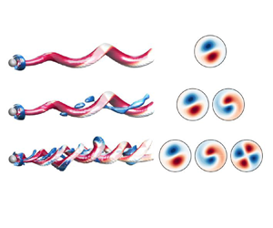
In the presence of supercritical self-sustained instabilities, rotating waves are predominant. These patterns prevail in axisymmetric flows, where the reflection symmetry regarding the azimuthal angle is broken. Here, the reflection symmetry is broken because of the rotation of the sphere, which induces a preferential direction of rotation. Consequently, bifurcations that lead to standing waves or to a symmetry breaking steady state do not occur generically. The existence of standing waves or a steady-state mode requires the matching between the phase speed of the helical pattern and the rotation of the body, which is another condition to be met. The global stability analysis of the flow past the sphere confirms that only rotating waves are linearly unstable for the range of Reynolds numbers  $\mbox { {Re}} < 300$ and $\varOmega < 4$. The parametric linear stability study of the flow past the rotating sphere shows the existence of three neutral curves, which are associated to the three least stable modes identified by global stability analysis. These correspond to rotating waves, named $RW_1$, $RW_2$ and $RW_3$, which are depicted in figure 2. Linear stability results (figure 3a) reveal that the axisymmetric steady state, referred in the following as a trivial state, is stable in the white shaded region and unstable in the grey shaded region. The neutral curve of stability displays two regions in the parameter space $(\mbox { {Re}}, {{\varOmega }})$ for which the first primary bifurcations are rotating waves of low frequency where the wake past the sphere displays a single helix ( $RW_1$), depicted in figure 2(a). In the second region, the flow pattern of the wake displays a double helix ( $RW_3$) with a high frequency, depicted in figure 2(c). The onset of instability of the third branch ( $RW_2$) displaying a flow pattern of the wake with a single helix with a medium frequency, depicted in figure 2(b), turns out to be linearly unstable for $\varOmega \leq 4$. Each pair of neutral curves intersects once, leading to three codimension-two points (
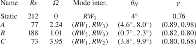
 $A$,
$A$,  $B$,
$B$,  $C$), identified in table 1. Another aspect of importance is the evolution of frequencies of the instability. Frequencies at critical parameters are reported in figure 3(b) as a function of ${{\varOmega }}$. The frequency evolution is divided into two regions, a first of rapid evolution for low rotation rates ${{\varOmega }} < 1$ and a second where the frequency of the three modes hardly depends on the rotation rate.
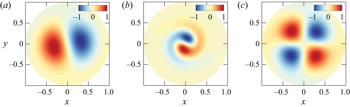
Figure 2. Cross-section view at  $z=3.5$ of the three unstable modes. The streamwise component of the vorticity vector $\varpi _z$ is visualized by colours. Results are shown for (a) $RW_1$ at point $(\mbox { {Re}}_A, \varOmega _A) = (77,2.24)$; (b) $RW_2$ at point $(\mbox { {Re}}_B, \varOmega _B)=(188,1.01)$; (c) $RW_3$ at point $(\mbox { {Re}}_A, \varOmega _A)$.
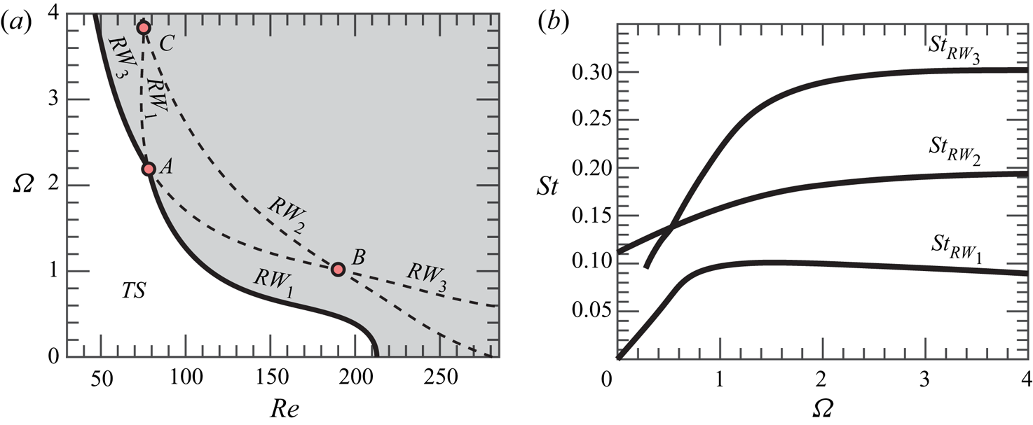
Figure 3. Linear stability properties of the rotating sphere configuration. (a) Neutral curve of stability: the onset of the primary instability is portrayed with a solid black line ( $\textbf {---}$), whereas the continuation of the neutral curves is depicted with dashed black lines ( $\textbf {- - -}$). (b) Frequency evolution with respect to ${{\varOmega }}$ of linear modes at the critical Reynolds number ( $\mbox { {Re}}_c({{\varOmega }}$)).
Table 1. Location in the parameter space  $(\mbox { {Re}},{{\varOmega }}$) and the pair of modes involved at the codimension-two points. It also lists the main properties of the primary bifurcation of the flow past the static sphere. The last two columns are related to non-normality effects and are defined in § 3.3.
The neutral curve of stability reveals that the static configuration ( $\varOmega = 0$) exhibits the largest critical Reynolds number. Then, the critical value of the Reynolds number is hardly modified by weak rotating speeds, in the range ${{\varOmega }} < 0.3$. However, there is a clear threshold around ${{\varOmega }} \approx 0.4$ where the critical Reynolds number passes from around $\mbox { {Re}}_c \approx 200$ to $\mbox { {Re}}_c \approx 100$ in a narrow interval ${{\varOmega }} \in [0.4, 1.2]$. The critical Reynolds number remains approximately constant up to the point $A$, the point which divides the boundary of stability. Below the point $A$, that is, for ${{\varOmega }} < {{\varOmega }}_A$, the steady-state flow transits supercritically to a single helix rotating wave $RW_{1}$; above the point $A$, i.e. ${{\varOmega }} > {{\varOmega }}_A$, the steady-state flow transits supercritically to the double helix rotating wave, $RW_{3}$. Such a point corresponds to a double-Hopf bifurcation between modes 1 and 3, and its analysis is left to §§ 4 and 5. Other two double-Hopf bifurcation points exist, denoted $B$ and $C$, which characterize the interaction between modes 2 and 3, and 1 and 2, respectively. Yet, at points $B$ and $C$ the trivial state is already unstable, thus, instabilities associated with these points are not directly observed in experiments or numerical simulations. Instead, these organizing centres play a role in the pattern formation of secondary instabilities, which is left to §§ 4 and 5, where we interpret the subtle implications of these points in dynamics. In addition, authors have looked for the presence of a primary bifurcation that leads to the $RW_{2}$ state. For the studied configuration, there does not exist such a region in the range $0 < {{\varOmega }} < 6$.
3.3. Properties of the axisymmetric steady state
The analysis presented in this section studies the linear stability of the axisymmetric steady-state solution in the range  $\mbox { {Re}} \leq 250$ and $\varOmega \leq 4$. Typical axisymmetric steady-state solutions (TS) at codimension-two points are portrayed in figure 4, which shows the neutrally stable trivial state state at $(Re_A,\varOmega _A)=(77,2.24)$ and the two other unstable trivial states at $(Re_B,\varOmega _B)=(188,1.01)$ and $(Re_C,\varOmega _C)=(73,3.95)$, respectively. The flow visualization illustrates the recirculation region behind the sphere, delimited by the separatrix, which divides the recirculation bubble and the unperturbed flow field. Such a line, depicted with a thick solid line in figure 4 connects the separation point on the sphere surface and the stagnation point on the $r=0$ axis. The development of the recirculation bubble can be measured using the maximum extent of the region
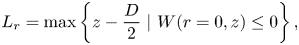 \begin{equation} L_r = \max \left\{ z - \frac{D}{2} \text{ } |\text{ } W(r=0,z) \leq 0 \right\}, \end{equation}
where  $D$ is the diameter of the sphere. Figure 5(a) displays the evolution of the length of the recirculation bubble by varying $\varOmega$ and $\mbox { {Re}}$. The length of the bubble increases monotonically with the angular velocity $\varOmega$ of the sphere as well as the largest negative values of the streamwise velocity behind the sphere, from around $40\,\%$ for $\varOmega = 0$ to around $60\,\%$ for the largest values of $\varOmega$ explored. A similar trend was identified by Kim & Choi (Reference Kim and Choi2002) at $Re$=100; however, we should consider that the trends observed in figure 5(a) are only valid before bifurcation. After that, $L_r$ does not have to increase with $\varOmega$, as seen by Lorite-Díez & Jiménez-González (Reference Lorite-Díez and Jiménez-González2020) and Kim & Choi (Reference Kim and Choi2002). The results at the onset of stability of the steady state are synthesized in figure 5(b), with a domain of existence of a stable steady state (white shaded) and another of an unstable steady state (grey shaded). In § 3.4 we identify the core of the $RW_1$ and $RW_3$ instabilities, which are found within the recirculation region. In particular, a passive control that shortens the recirculation region is an efficient technique to stabilize the flow. Therefore, it is not surprising that the neutrally stable flow is characterized by a shorter recirculation region with respect to the unstable steady state.
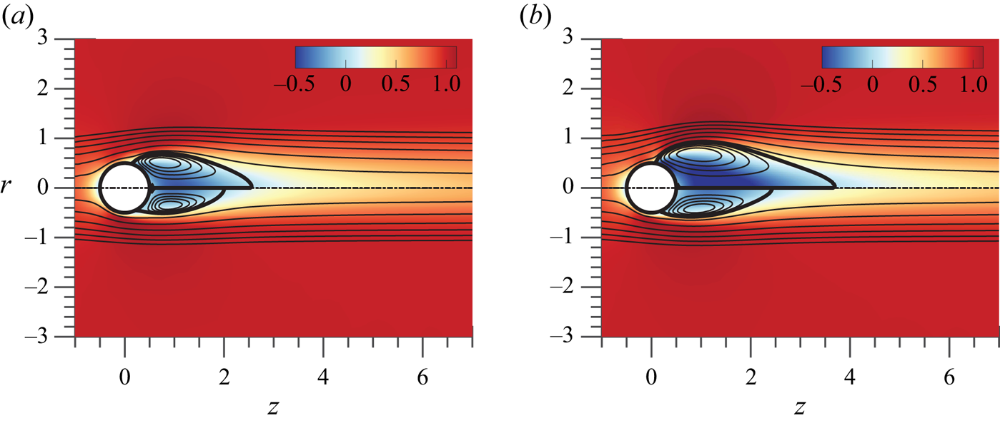
Figure 4. Spatial distribution of the streamwise velocity (contours) at the steady state along with flow streamlines (solid lines) and recirculation region separatrix (thick solid lines). Results are shown for (a)  $(\mbox { {Re}} = 212, \varOmega = 0)$ in the upper half and $(\mbox { {Re}}_A, \varOmega _A)$ in the lower half; (b) $(\mbox { {Re}}_B, \varOmega _B)$ in the upper half and $(\mbox { {Re}}_C, \varOmega _C)$ in the bottom half. Points $A$,
$A$,  $B$ and $C$ are defined in table 1.
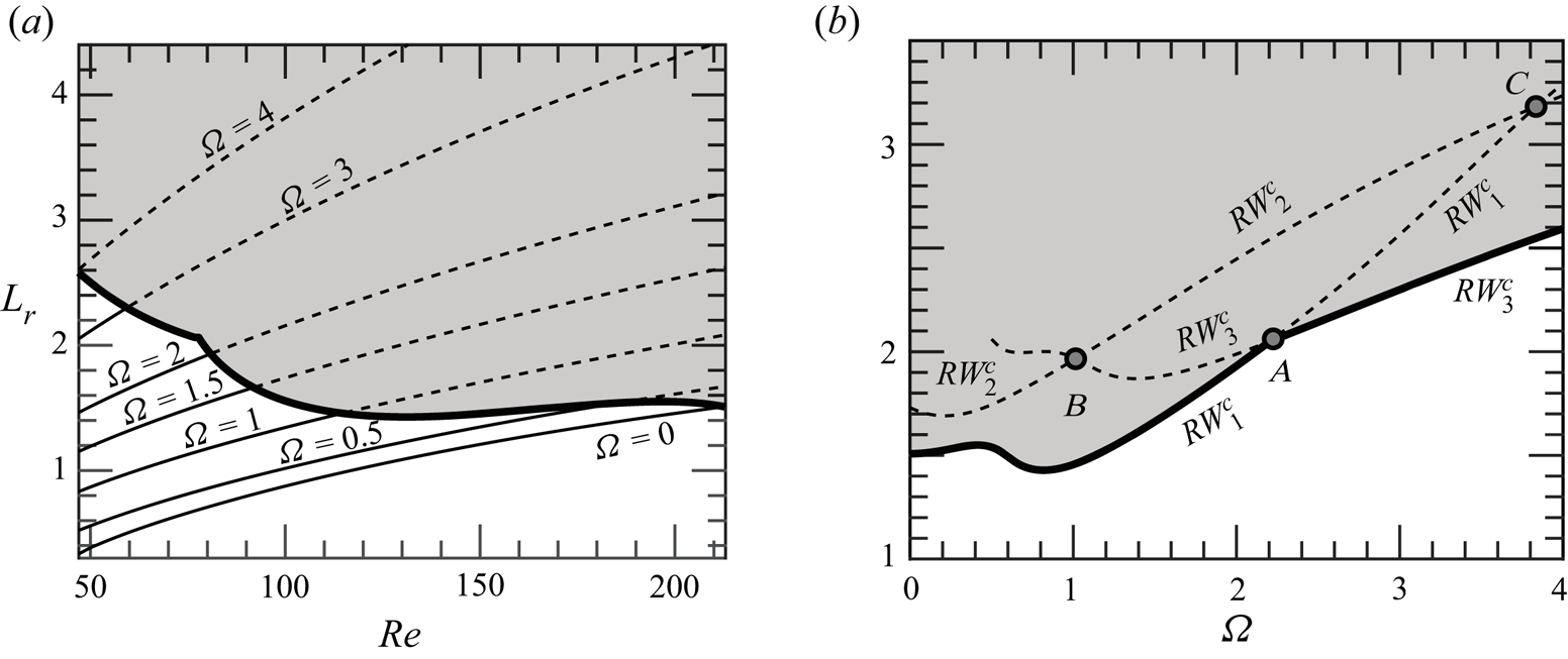
Figure 5. Evolution of the recirculating length  $L_r$ in the plane $(\mbox { {Re}}, {{\varOmega }})$. The unstable region is the grey-shaded area, delimited by a thick line. (a) The recirculating length of the stable solution is painted with solid lines, dashed lines are employed for the unstable steady state. (b) Length of the recirculating region at the onset of stability $(\mbox { {Re}}_c(\varOmega ))$.
Finally, we briefly discuss the influence of non-normality mechanisms, lift-up and convective non-normality as they are partly related to recirculation region length. The main results are included in table 1, where we can see a lower influence of non-normality effects through the obtained values for  $\gamma$ and $\theta _{N}$, with respect to the static sphere configuration. The estimator $\theta _N$ measures the importance of non-normality, the lower $\theta _N$ the more important non-normal effects are. On the other hand, the estimator $\gamma$ characterizes the relative contribution between the lift-up and the convective non-normality mechanisms to the total non-normality effects. A $\gamma$ value close to $0$ indicates the dominance of the lift-up effect. The largest non-normal effects have been measured at point $B$ (lowest values of $\theta _N$), which corresponds to the point with the largest critical Reynolds number among the codimension-two points. The values of $\theta _N$ obtained at point $B$ are associated with a larger non-normality than the stationary mode (the case of $RW_1$ with $O(2)$ symmetry) and $RW_2$ at the threshold for $(\varOmega = 0, \mbox { {Re}} = 281)$, which was found by Meliga, Chomaz & Sipp (Reference Meliga, Chomaz and Sipp2009b) to be $1^{\circ }$. Thus, one may conclude that the rotation of the sphere increases the effect of non-normality, however, it induces an earlier transition with regard to the Reynolds number, which turns out to globally reduce the effect of non-normality. This previous statement can be also indirectly verified from the satisfactory comparison between normal form estimations and DNS results in § 5.1. Furthermore, the analysis of the direct global mode shows a dominant effect of the convective non-normality, which is responsible at most of around $90\,\%$ (mode $RW_1$) and $98\,\%$ (mode $RW_3$) at point $A$ and around $80\,\%$ for the remainder modes at points $B$ and $C$. In comparison, the stationary and oscillating modes of static configuration ( $\varOmega = 0$) displayed $\gamma = 0.76$ and $\gamma = 0.94$. More details about the non-normality study such as the definition of $\theta _N$ and $\gamma$ can be found in Appendix B.
3.4. Identification of the physical mechanisms from a control perspective
In this section we analyse the physical mechanisms leading to the  $RW_1$ and $RW_3$ states at the point $A$. However, we do not discuss the $RW_2$ state as it will be seen in § 5, this state is not expected to be observed. First, we consider what is the effect of a steady axisymmetric forcing term, which represents the presence of a small obstacle, wall suction/blowing (as the control applied in Niazmand & Renksizbulut Reference Niazmand and Renksizbulut2005), etc. In this case the governing equations of the resulting flow are the same as (2.3) with the addition of a forcing term $\boldsymbol {H}_0 \equiv \boldsymbol {\hat {H}}_0$,
 \begin{equation} \boldsymbol{B} \frac{\partial \boldsymbol{Q}}{\partial t} = \boldsymbol{F}(\boldsymbol{Q}, \boldsymbol{\eta}) \equiv \boldsymbol{L} \boldsymbol{Q} + \boldsymbol{N}(\boldsymbol{Q},\boldsymbol{Q}) + \boldsymbol{G} (\boldsymbol{Q},\boldsymbol{\eta}) + \boldsymbol{\hat{H}}_0. \end{equation}
 This case has been treated in the past by Marquet, Sipp & Jacquin (Reference Marquet, Sipp and Jacquin2008) in the case of the flow past a circular cylinder and by Sipp (Reference Sipp2012) in the case of the open cavity flow. The introduction of the forcing induces a modification of the eigenvalue  $\mathrm {i} \omega _{\ell } \mapsto \mathrm {i} \omega _{\ell } + \Delta \mathrm {i} \omega _{\ell }^{0}$, where $\Delta \mathrm {i} \omega _{\ell }^{0} = \langle {\boldsymbol {\nabla }_{\boldsymbol {H}_{0}} \mathrm {i} \omega _{\ell } } , {\boldsymbol {\hat {H}}} \rangle$. Therefore, the control that induces the largest deviation of the growth rate (respectively frequency) of the mode $\ell$ is in the direction of $\boldsymbol {\nabla }_{\boldsymbol {H}_{0}} \mathrm {i} \omega _{\ell }$, which is defined as
 \begin{equation} \boldsymbol{\nabla}_{\boldsymbol{H}_{0}} \mathrm{i} \omega_{\ell} = \boldsymbol{B}^{\rm T} \boldsymbol{J}_{(0,0)} \boldsymbol{B} \boldsymbol{\nabla}_{\boldsymbol{U}_b} \mathrm{i} \omega_{\ell}\quad \text{for } \ell = 1,2,3. \end{equation}
Here  $\boldsymbol {\nabla }_{\boldsymbol {U}_b} \mathrm {i} \omega _{\ell }$ is the sensitivity of the eigenvalue of the mode $\ell$ ( $\ell = 1,2,3$) with respect to variations in the axisymmetric steady state, cf. (Marquet et al. Reference Marquet, Sipp and Jacquin2008). The sensitivity of the $\ell ^{th}$ eigenvalue $\boldsymbol {\nabla }_{\boldsymbol {H}_{0}} \lambda _{\ell }$ to the introduction of a steady axisymmetric forcing is represented in figure 6 for the two modes present in the codimension point $A$. The low-frequency mode ( $RW_1$) is most sensitive to a steady axisymmetric forcing at the leftmost end of the recirculation region (see figure 6a,b). This forcing corresponds to one that accelerates the streamwise motion at the end of the recirculation region, thus reducing the counterclockwise motion of the recirculation zone, which would induce an effective decrease of the growth rate (respectively frequency). This is in accordance with the fact that the recirculation motion will be weaker, and the convective motion will be slower (note this is also the case for the sensitivity of the frequency $RW_3$ to steady forcing figure 6d). On the other hand, the high-frequency mode is most sensitive in a near wake region behind the sphere, close to the recirculation bubble (see figure 6c,d). In this case, a forcing that decelerates the clockwise motion within the recirculation region would cause the largest stabilization effect.
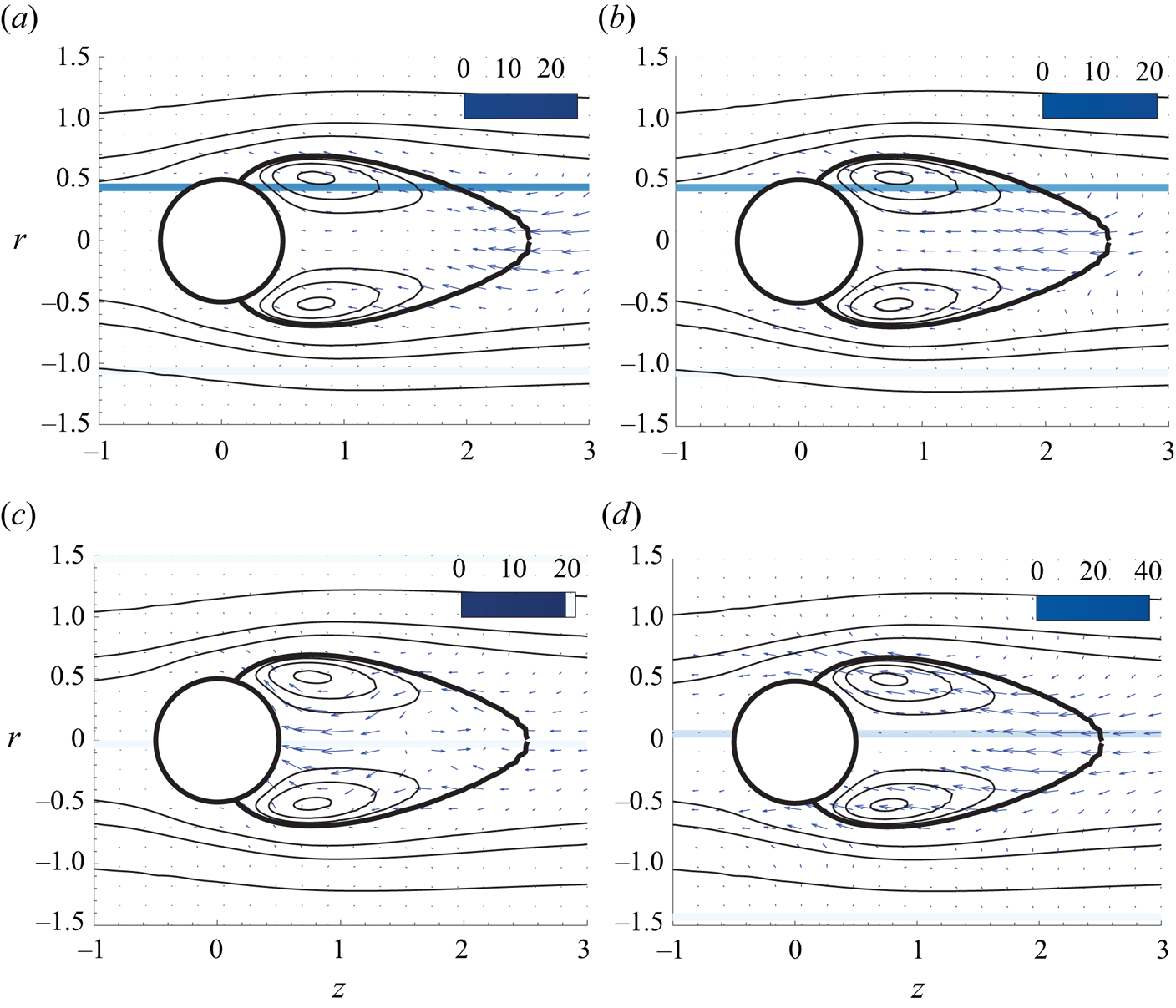
Figure 6. Steady forcing at codimension point  $A$. Sensitivity of amplification rate to the steady axisymmetric forcing $\boldsymbol {\nabla }_{\boldsymbol {H}_{0}} \lambda _{\ell }$ for (a) the low-frequency mode, also known as $RW_1$, and (c) the high-frequency mode, also known as $RW_3$. Sensitivity of the frequency to the steady axisymmetric forcing $\boldsymbol {\nabla }_{\boldsymbol {H}_{0}} \lambda _{\ell }$ for (b) the low-frequency mode, $RW_1$, and (d) the high-frequency mode, $RW_3$. The magnitude of the growth rate and frequency sensitivities is pictured by colours and their orientation by arrows.
Second, let us consider the receptivity of the flow to the presence of localized feedbacks, as in Giannetti & Luchini (Reference Giannetti and Luchini2007). The harmonic forcing  $\boldsymbol {H} \equiv \boldsymbol {H}_{(z_{\ell })} \exp ({\mathrm {i} (\omega _{\ell } t + m_{\ell } \theta )})$ is defined as
 \begin{equation} \boldsymbol{H}_{(z_{\ell})} = \delta(\boldsymbol{x} - \boldsymbol{x}_0) \boldsymbol{C}_{(z_{\ell})} \boldsymbol{\cdot} \hat{\boldsymbol{u}}_{(z_{\ell})}, \quad \ell = 1,2,3, \end{equation}
where  $\boldsymbol {C}_{(z_{\ell })}$ is a generic feedback matrix and $\delta (\boldsymbol {x} - \boldsymbol {x}_0)$ is the Dirac distribution centred at the point $\boldsymbol {x}_0 = (z_0, r_0, \theta _0)$. Thus, the variation of the eigenvalue due to the introduction of the localized feedback is
 \begin{equation} \Delta^{u} \mathrm{i} \omega_{\ell} = \langle {\hat{\boldsymbol{q}}_{(z_{\ell})}^{{{{\dagger}}}}} , {\delta \boldsymbol{H}_{(z_{\ell})} } \rangle = \boldsymbol{C}_{(z_{\ell})} : {\boldsymbol{\mathsf{S}}}_s^{({\ell})} (\boldsymbol{x}_0) , \quad \ell \in \textrm{I} \end{equation}
 The rank two tensor of (3.7) is commonly designated as the structural sensitivity tensor, here denoted as  ${\boldsymbol{\mathsf{S}}}_s^{({\ell })}$,
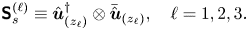 \begin{equation} {\boldsymbol{\mathsf{S}}}_s^{({\ell})} \equiv \hat{\boldsymbol{u}}_{(z_{\ell})}^{{{{\dagger}}}} \otimes \bar{\hat{\boldsymbol{u}}}_{(z_{\ell})}, \quad \ell = 1,2,3. \end{equation}
 The spectral norm of the structural sensitivity tensor for low- and high-frequency modes is depicted in figure 7. Similar to the receptivity to axisymmetric steady forcing, the recirculation bubble ( $RW_3$) and the leftmost end of the recirculation region ( $RW_1$) are the most sensitive regions of the flow.
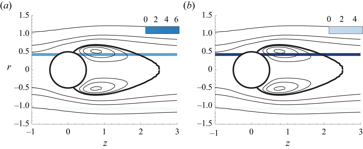
Figure 7. Spectral norm of the structural sensitivity tensor. (a) Low-frequency mode, (b) high-frequency mode.
4. Normal form reduction
In this study bifurcations involving a steady-state mode uniquely exist for the static configuration ( ${{\varOmega }} = 0$). For such a reason, we will focus our attention on the codimension-two double-Hopf (Chossat, Golubitsky & Lee Keyfitz Reference Chossat, Golubitsky and Lee Keyfitz1986) and the codimension-three triple-Hopf bifurcations, and we will characterize solutions based on the patterns allowed by these bifurcations. In our problem, the competition between two or more of the several rotating waves occurs in the neighbourhood of the primary bifurcation. For such a reason, the three double-Hopf points (depicted in figure 3a) are of special interest.
These points act as organizing centres of dynamics, and they provide some partial answers about the transition scenario. For instance, around the point  $A$ there are regions of bi-stability where either $RW_1$ and $RW_3$ coexist. Nevertheless, these codimension-two points do not account for a third interaction. In each of the double-Hopf interactions, the competition with one of the leading modes is omitted. The full instability scenario is accounted by considering the unfolding of the triple-Hopf bifurcation. Yet, such an instability does not show up generally with only two parameters. And the search for a third parameter where such a bifurcation generically occurs is not a trivial task. Not to mention that even in the case one finds such a parameter, the flow configuration may be considerably distinct from the one initially conceived. Therefore, in the current research, we adopt a similar strategy as the one conducted by Meliga et al. (Reference Meliga, Chomaz and Sipp2009a) on the wake flow past a disk. However, rather than performing a variation of the centre-unstable manifold reduction, which is an invariant procedure but without the attractiveness property of the centre manifold (Podvigina Reference Podvigina2006a,Reference Podviginab), we prefer to adopt a higher-order (up to fifth order) multiple scales expansion at each codimension-two point, and then we extend the coefficients to other locations in the parameter space. The chosen approach differentiates from other previous techniques because it allows an exact identification of the polynomial coefficients of the normal form at codimension-two points, where one can employ the Fredholm alternative to determine the normal form coefficients and remove the secular terms of the expansion. Other centre-unstable techniques determine the coefficients of the normal form at non-resonant conditions, which invalidates the use of the Fredholm alternative if one is far from the onset of instability. On the other hand, our technique does not provide an a priori knowledge of the error committed in the extension procedure from a codimension-two point to another point in the parameter space. Thus, as with other perturbative techniques, one needs to perform a cross-comparison with DNS in the region of interest of the parameter space, which is performed in § 5.1.
In the following, we briefly outline the main constituents in the study of pattern formation, a comprehensive explanation is left to Appendix A. Pattern formation is studied herein in the framework of bifurcation theory. Near the onset of the bifurcation, dynamics can be reduced to the centre manifold, whose algebraic expression is simplified via a series of topologically equivalent transformations into the normal form. The reduction to the normal form is carried out via a multiple scales expansion of the solution  $\boldsymbol {Q}$ of (2.3). The expansion considers a two-scale development of the original time $t \mapsto t + \varepsilon ^{2} \tau$, here $\varepsilon$ is the order of magnitude of the flow disturbances, assumed small $\varepsilon \ll 1$. In this study we carry out a normal form reduction via a weakly nonlinear expansion, where the small parameters are
 \begin{equation} \varepsilon_{{{\varOmega}}}^{2} = \left({{\varOmega}}_c - {{\varOmega}} \right) \sim \varepsilon^{2} \quad \text{and}\quad \varepsilon_{\nu}^{2} = \left( \nu_c - \nu \right) = \left( \mbox{{Re}}_c^{{-}1} - \mbox{{Re}}^{{-}1} \right) \sim \varepsilon^{2}. \end{equation}
The technique decomposes time into a fast time scale  $t$ of the phase associated to the self-sustained instabilities and a slow time scale related to the evolution of the amplitudes $z_i(\tau )$, introduced in (4.3), for $i=1,2,3$. The ansatz of the expansion is
 \begin{equation} \displaystyle \boldsymbol{Q}(t,\tau) = \boldsymbol{Q}_b + \varepsilon \boldsymbol{q}_{(\varepsilon)}(t,\tau) + \varepsilon^{2} \boldsymbol{q}_{(\varepsilon^{2})}(t,\tau) + \varepsilon^{3} \boldsymbol{q}_{(\varepsilon^{3})}(t,\tau) + \varepsilon^{4} \boldsymbol{q}_{(\varepsilon^{4})}(t,\tau) + O(\varepsilon^{5}). \end{equation}
In the following, we shall consider the normal form equation resulting from the interaction of three rotating wave modes identified by LSA, that is,
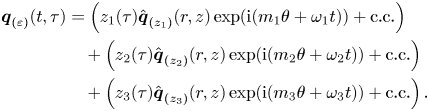 \begin{align} \boldsymbol{q}_{(\varepsilon)}(t,\tau) & = \left( z_1(\tau) \hat{\boldsymbol{q}}_{(z_{1})}(r,z) \exp({\mathrm{i}( m_1 \theta + \omega_1 t)}) + \text{c.c.} \right)\nonumber\\ &\quad + \left( z_2(\tau) \hat{\boldsymbol{q}}_{(z_{2})}(r,z) \exp({\mathrm{i} (m_2 \theta + \omega_2 t)}) + \text{c.c.} \right)\nonumber\\ &\quad + \left( z_3(\tau) \hat{\boldsymbol{q}}_{(z_{3})}(r,z) \exp({\mathrm{i} (m_3 \theta + \omega_3 t)}) + \text{c.c.} \right). \end{align}
Note that the expansion of the left-hand side of (2.3) up to fifth order is
 \begin{align} \displaystyle \varepsilon \boldsymbol{B} \frac{\partial \boldsymbol{q}_{(\varepsilon)}} {\partial t} + \varepsilon^{2} \boldsymbol{B} \frac{\partial \boldsymbol{q}_{(\varepsilon^{2})}} {\partial t} + \varepsilon^{3} \left[ \boldsymbol{B} \frac{\partial \boldsymbol{q}_{(\varepsilon^{3})}} {\partial t} + \boldsymbol{B} \frac{\partial \boldsymbol{q}_{(\varepsilon)}} {\partial \tau} \right] + \varepsilon^{4} \boldsymbol{B} \frac{\partial \boldsymbol{q}_{(\varepsilon^{4})}} {\partial t} + \varepsilon^{5} \left[ \boldsymbol{B} \frac{\partial \boldsymbol{q}_{(\varepsilon^{3})}} {\partial \tau} \right] + O(\varepsilon^{5}), \end{align}
and the right-hand side respectively is
 \begin{equation} \boldsymbol{F} (\boldsymbol{q}, \boldsymbol{\eta}) = \boldsymbol{F}_{(0)} + \varepsilon \boldsymbol{F}_{(\varepsilon)} + \varepsilon^{2} \boldsymbol{F}_{(\varepsilon^{2})} + \varepsilon^{3} \boldsymbol{F}_{(\varepsilon^{3})} + \varepsilon^{4} \boldsymbol{F}_{(\varepsilon^{4})} + \varepsilon^{5} \boldsymbol{F}_{(\varepsilon^{5})} + O(\varepsilon^{6}). \end{equation}
Then, the problem truncated at order three is reduced to a low-dimensional system governing the complex amplitudes  $z_j(t)$,
 \begin{equation} \left. \begin{aligned} \dot{z_1} & = z_1 \left[\lambda_1 + \nu_{11}|z_1|^{2} + \nu_{12}|z_2|^{2} + \nu_{13}|z_3|^{2}\right],\\ \dot{z_2} & = z_2 \left[\lambda_2 + \nu_{21}|z_1|^{2} + \nu_{22}|z_2|^{2} + \nu_{23}|z_3|^{2}\right], \\ \dot{z_3} & = z_3 \left[\lambda_3 + \nu_{31}|z_1|^{2} + \nu_{32}|z_2|^{2} + \nu_{33}|z_3|^{2}\right], \end{aligned} \right\} \end{equation}
where  $\nu _{k \ell }, \lambda _k \in \mathbb {C}$ for $k, \ell =1,2,3$. The real part of the linear terms, named $\lambda _k$, correspond to the growth rate of the $k^{th}$ mode. Respectively, the imaginary part of $\lambda _k$ is associated to the frequency variation of the $k^{th}$ mode with respect to the frequency of the neutral mode, i.e. with respect to the frequency $\omega _k$ determined from LSA. The terms $\nu _{k \ell }$ are the third-order self ( $k=\ell$) and cross-interaction $(k\neq \ell )$ coefficients. The coefficients of the normal form are estimated as
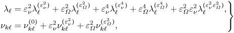 \begin{equation} \left. \begin{aligned} \lambda_{\ell} & = \varepsilon_{\nu}^{2} \lambda_{\ell}^{(\varepsilon_{\nu}^{2})} + \varepsilon_{{{\varOmega}}}^{2} \lambda_{\ell}^{(\varepsilon_{{{\varOmega}}}^{2})} + \varepsilon_{\nu}^{4} \lambda_{\ell}^{(\varepsilon_{\nu}^{4})} + \varepsilon_{{{\varOmega}}}^{4} \lambda_{\ell}^{(\varepsilon_{{{\varOmega}}}^{4})} + \varepsilon_{{{\varOmega}}}^{2}\varepsilon_{\nu}^{2} \lambda_{\ell}^{(\varepsilon_{\nu}^{2} \varepsilon_{{{\varOmega}}}^{2})},\\ \nu_{k \ell} & = \nu_{k \ell}^{(0)} + \varepsilon_{\nu}^{2} \nu_{k \ell}^{(\varepsilon_{\nu}^{2})} + \varepsilon^{2}_{{{\varOmega}}} \nu_{k \ell}^{(\varepsilon_{{{\varOmega}}}^{2})}, \end{aligned} \right\} \end{equation}
where  $\nu _{k \ell }^{(0)}, \nu _{k \ell }^{(\varepsilon _{\nu }^{2})}$, $\nu _{k \ell }^{(\varepsilon _{{{\varOmega }}}^{2})}$, and the corresponding linear coefficients, are evaluated at the intersection point between the Hopf curves associated to mode $k$ and $\ell$. For instance, the coefficient $\nu _{1 3}^{(0)}$ is evaluated at point $A$. The distinct coefficients of (4.7) used for the evaluation of the coefficients of the normal form are listed in tables 4 and 5 (Appendix A).
4.1. Classification of solutions
In the following, the right-hand side of (4.6) is designated  $\boldsymbol {f}(\boldsymbol {z})$ where $\boldsymbol {z} = (z_1,z_2,z_3)$. The reduced vector $\boldsymbol {f}$ is equivariant under the action of the group $\varGamma \equiv SO(2) \times \mathbb {T}^{3}$, with the following action representation:
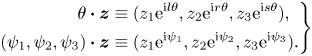 \begin{equation} \left. \begin{aligned} \theta \boldsymbol{\cdot} \boldsymbol{z} & \equiv (z_1 {\rm e}^{{\rm i} l\theta},z_2 {\rm e}^{{\rm i} r\theta},z_3 {\rm e}^{{\rm i} s\theta}),\\ (\psi_1,\psi_2,\psi_3) \boldsymbol{\cdot} \boldsymbol{z} & \equiv (z_1 {\rm e}^{{\rm i} \psi_1},z_2 {\rm e}^{{\rm i} \psi_2},z_3 {\rm e}^{{\rm i} \psi_3}). \end{aligned} \right\} \end{equation}
Here  $l,r,s \in \mathbb {Z}$, $\theta \in [0, 2{\rm \pi} )$ and $\psi _i \in [0,2{\rm \pi} )$ for $i = 1,2,3$; $(\psi _1,\psi _2,\psi _3)$ and $\theta$ are the representations in $\mathbb {C}^{3}$ of the actions of the group $\varGamma$, which correspond to the time shift and rotational invariance, respectively. The substitution of the polar decomposition of $\boldsymbol {z} = \boldsymbol {r} \textrm {e}^{\textrm {i} \boldsymbol {\varPhi } }$, with $\boldsymbol {r} = (r_1,r_2,r_3 )$ and $\boldsymbol {\varPhi } = ( \phi _1, \phi _2, \phi _3 )$, into (4.6) yields the following decoupled phase-amplitude system:
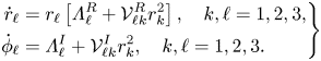 \begin{equation} \left. \begin{aligned} \dot{{r}}_{\ell} & = r_{\ell} \left[ \varLambda^{R}_{\ell} + \mathcal{V}^{R}_{\ell k} {r}^{2}_{k} \right], \quad k,\ell = 1,2,3,\\ \dot{\phi}_{\ell} & = \varLambda^{I}_{\ell} + \mathcal{V}^{I}_{\ell k} {r}^{2}_k, \quad k,\ell = 1,2,3. \end{aligned} \right\} \end{equation}
Here  $\varLambda = \varLambda ^{R} + \varLambda ^{I} \equiv (\lambda _1,\lambda _2,\lambda _3)^\textrm {T}$ and the matrix $\mathcal {V} = \mathcal {V}^{R} + \textrm {i} \mathcal {V}^{I}$ is
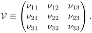 \begin{equation} \mathcal{V} \equiv \begin{pmatrix} \nu_{11} & \nu_{12} & \nu_{13} \\ \nu_{21} & \nu_{22} & \nu_{23} \\ \nu_{31} & \nu_{32} & \nu_{33} \end{pmatrix}. \end{equation}
 To ease the presentation of the fixed-point solutions of (4.9), let us introduce the inverse of the linear operator  $\mathcal {V}$, which can be written as
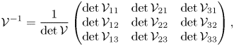 \begin{equation} \mathcal{V}^{{-}1} = \dfrac{1}{\det{\mathcal{V}}} \begin{pmatrix} \det{\mathcal{V}}_{11} & \det{\mathcal{V}}_{21} & \det{\mathcal{V}}_{31} \\ \det{\mathcal{V}}_{12} & \det{\mathcal{V}}_{22} & \det{\mathcal{V}}_{32} \\ \det{\mathcal{V}}_{13} & \det{\mathcal{V}}_{23} & \det{\mathcal{V}}_{33} \end{pmatrix}, \end{equation}
where  $\det {\mathcal {V}}_{k\ell }$ denotes the minor of the matrix $\mathcal {V}$, obtained by eliminating the line $k$ and the column $\ell$.
In the following, the notation  $\dot {\boldsymbol {r}} = \boldsymbol {f}^{R}( \boldsymbol {r} )$ will be adopted to denote the amplitude equation of the nonlinear system (4.9). The remainder of this subsection will be devoted to the study of the three fixed-point solutions of (4.9).
The classification of the solutions of the generic triple-Hopf bifurcation interaction with  $SO(2)$ symmetry is based on maximal isotropy subgroups of the group $\varGamma$. This technique predicts the existence up to tertiary bifurcations of fixed points of the complex normal form (4.6). These isotropy subgroups correspond to the symmetries of the solutions within the fixed-point subspace of each isotropy group (cf. table 2).
Table 2. Nomenclature and symmetry group of fixed-point solutions of the system (4.9).
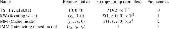
In our discussion, we identify the subgroups of  $SO(2) \times \mathbb {T}^{3}$. Each element in the group has the form
 \begin{equation} (\theta, \psi_1, \psi_2, \psi_3) \in SO(2) \times \mathbb{T}^{3}. \end{equation}
Using this notation, the subgroup  $S(k,l,r,s)$ of $SO(2) \times \mathbb {T}^{3}$ is defined as
 \begin{equation} S(k,l,r,s) = \{ (k \theta, l \theta, r \theta, s \theta ) | \theta \in S^{1} \}. \end{equation}
The conjugacy classes of isotropy subgroups of  $SO(2) \times \mathbb {T}^{3}$ are documented with the representative of the fixed-point subspace in polar coordinates and the number of incommensurate frequencies in table 2. Additionally, a graphical representation of the isotropy lattice is displayed in figure 8 in terms of the class representative of the fixed-point subspace.

Figure 8. Isotropy lattice of the triple-Hopf bifurcation.
Rotating waves correspond to the simplest non-trivial fixed point of (4.9), which in the original set of equations is a periodic solution. They arise as the result of a supercritical Hopf bifurcation of the steady state (named trivial state in table 2) and they may eventually bifurcate into mixed modes; the eigenvalues of rotating waves may be found in the first row of table 3. Mixed modes, defined in table 3, are the result of the interaction between two rotating waves. A mixed mode has a representative in the normal form with two non-zero amplitude terms, thus, they correspond to a  $T^{2}$-quasiperiodic state in the original system of equations. These states may experience two kinds of bifurcations. They may lose stability in the transversal direction or within their own subspace, these two conditions are listed in table 3. Eventually, a bifurcation in the transversal direction of a mixed mode may be associated with the appearance of an interacting mixed mode ( $IMM_{123}$) attractor. An interacting mixed mode corresponds to a $T^{3}$-quasiperiodic state in the original system of equations, and it is represented by three non-zero amplitude terms. However, $T^{3}$-quasiperiodic states are hardly observed in numerical simulations of dissipative systems, as it is the case of Navier–Stokes equations (2.1), instead a chaotic attractor is usually detected. A more exhaustive analysis of the unfolding of the triple-Hopf bifurcation is left to Appendix C.
Table 3. Defining equations and eigenvalues of the solutions of the polar third-order normal form (4.9).
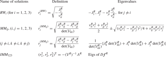
4.2. Illustration of the procedure
Let us detail the procedure followed to compute the bifurcation scenario, a procedure that is also followed in § 5 for the determination of the parametric portrait. For the sake of simplicity, we first discuss the bifurcation diagram for a constant rotation rate  $\varOmega = 1.75$ in terms of the amplitudes $(r_1, r_2, r_3)$. We would like to remind the reader that the amplitudes $(r_1, r_2, r_3)$ are representative of the kinetic energy of the velocity fluctuations, based on the normalization choice of § 3.1. First, we need to determine the coefficients of the normal form, listed in tables 4 and 5, following the procedure of Appendix A. Then, one may evaluate the linear and cubic coefficients of the normal form at $\varOmega = 1.75$ for a variable Reynolds number from the evaluation of (4.7). Please note that, for the evaluation of cross-diagonal cubic coefficients, the expansion parameter $\varepsilon _\varOmega ^{2} = \varOmega _c - \varOmega$ depends on the location of the critical rotation rate $\varOmega _c$, that is, to evaluate $\nu _{13}$ one evaluates $\varepsilon _{\varOmega,A}^{2} = \varOmega _{A} - \varOmega$ whereas to evaluate $\nu _{23}$ one evaluates $\varepsilon _{\varOmega,B}^{2} = \varOmega _{B} - \varOmega$. The diagonal cubic coefficients may be evaluated directly at the bifurcation point for every rotation rate $\varOmega$ as a function of $\varepsilon _\nu ^{2}$ or by considering the cubic coefficient of the nearest codimension-two point. In our procedure, we found good agreement with time-stepping simulations in the range $1 \leq \varOmega \leq 3$ if we consider $\nu _{11} = \nu _{11}^{A}$, $\nu _{22} = \nu _{22}^{B}$ and $\nu _{33} = \nu _{33}^{B}$; the consideration of $\nu _{33}^{A}$ induces a small deviation in the transition from $MM_{23}$ to $IMM_{123}$ of few units of the Reynolds number. The corresponding coefficients for $\varOmega = 1.75$ are listed in table 6 (Appendix A). Please note that the procedure illustrated herein corresponds to a method to determine the coefficients of the normal form; nonetheless, these coefficients can be estimated from numerical simulations as in Fabre et al. (Reference Fabre, Auguste and Magnaudet2008) or following a data-driven approach, cf. Callaham, Brunton & Loiseau (Reference Callaham, Brunton and Loiseau2022), Loiseau & Brunton (Reference Loiseau and Brunton2018) and Loiseau, Noack & Brunton (Reference Loiseau, Noack and Brunton2018). Bifurcation events are designated by their corresponding value of the Reynolds number $Re_{{state}_a}^{{state}_b}$, where $\textrm {state}_a$ stands for the simplest state that exists before the bifurcation and ${state}_b$ stands for the resulting state after the bifurcation. In addition, the notation $Re_{{state}_a}^{\sigma _k,s}$ indicates a bifurcation of the $\textrm {state}_a$ where the eigenvalue $\sigma _k$ ( $k=1,2,3$) has changed sign, $s$ indicates stabilization and $u$ indicates the change from stable to unstable of the referring eigenvalue/eigenmode pair. In the following, there is only a bifurcation of this kind, the one associated to the mixed mode $MM_{12}$ that is stabilized/destabilized because of a change of sign of the eigenvalue in the transversal direction ( $r_3$). Thus, we simplify the notation to $Re_{{state}_a}^{s}$ or $Re_{{state}_a}^{u}$.
Table 4. Linear coefficients of the normal form (4.9) evaluated at codimension-two points.
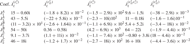
Table 5. Cubic coefficients of the normal form (4.9) evaluated at codimension-two points.
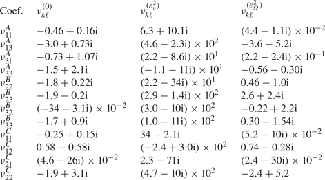
Table 6. Cubic coefficients of the normal form (4.9) evaluated at  $\varOmega = 1.75$.
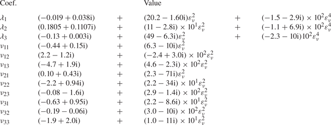
Figure 9 displays the bifurcation diagram, with Reynolds number as the control parameter for  $\varOmega = 1.75$. There exist three primary bifurcations, i.e. bifurcations from the axisymmetric steady state, located at $Re_{TS}^{RW_1}$, $Re_{TS}^{RW_2}$ and $Re_{TS}^{RW_3}$, respectively. However, the $RW_2$ branch remains unstable all along the analysed interval. The first transition to occur is a supercritical Hopf bifurcation leading to the $RW_1$ solution, which is then followed by another supercritical Hopf bifurcation leading to $RW_3$. For the range of Reynolds numbers $Re_{RW_1} < Re < Re_{RW_3}^{MM_{13}}$, there exists a single stable attractor, which corresponds to the limit cycle associated with the solution $RW_1$. At $Re_{RW_3}^{MM_{13}}$ the $RW_3$ branch experiences a Neimark–Sacker bifurcation that results in the appearance of the mixed-mode solution $MM_{13}$. In the interval $Re_{RW_3}^{MM_{13}} < Re < Re_{RW_1}^{MM_{13}}$ both primary solutions ( $RW_1$ and $RW_3$) are stable under any arbitrary perturbation and in addition they are connected by the unstable mixed mode $MM_{13}$, which is located on the separatrix of the basin of attraction of the two primary solutions, the phase portrait of this scenario is sketched in figure 9(b i). Eventually, the solution branch $MM_{13}$ terminates at $Re = Re_{RW_1}^{MM_{13}}$, which makes $RW_3$ the single attractor of the system for the interval $Re_{RW_1}^{MM_{13}} < Re < Re_{RW_3}^{MM_{23}}$. The $RW_3$ branch eventually bifurcates into the mixed-mode branch $MM_{23}$, which is a stable attractor within the interval $Re_{RW_3}^{MM_{23}} < Re < Re_{MM_{23}}^{IMM_{123}}$. The other primary branch, the unstable $RW_1$, undergoes another Neimark–Sacker bifurcation at $Re_{RW_1}^{MM_{12}}$ which results in the existence of the $MM_{12}$ branch, yet unstable for perturbations in the transversal direction of the mixed mode (in the $r_3$ direction). The $MM_{12}$ mixed-mode branch appears to be stable only within a small interval $Re_{MM_{12}}^{s} < Re < Re_{MM_{12}}^{u}$, where two bifurcations, which are associated to an instability in the transversal direction $r_3$, occur at the two limit values. We have employed $s$ and $u$ to denote the stable or unstable nature of the $MM_{12}$ regime. Thus, for $Re_{MM_{12}}^{s} < Re < Re_{MM_{12}}^{u}$, there is a second region with multiple stable attractors, which is schematically displayed in figure 9(b ii). The last bifurcation accounted by the normal form is the destabilization of the $MM_{23}$ branch at $Re = Re_{MM_{23}}^{IMM_{123}}$ that leads to the appearance of the $IMM_{123}$ branch, whose phase portrait is sketched in figure 9(b iii). Please note that despite the fact that $IMM_{123}$ is a fixed-point solution of the normal form, the Newhouse–Takens–Ruelle theorem indicates that the original system of equations may exhibit a chaotic attractors shadowing the $IMM_{123}$ solution.
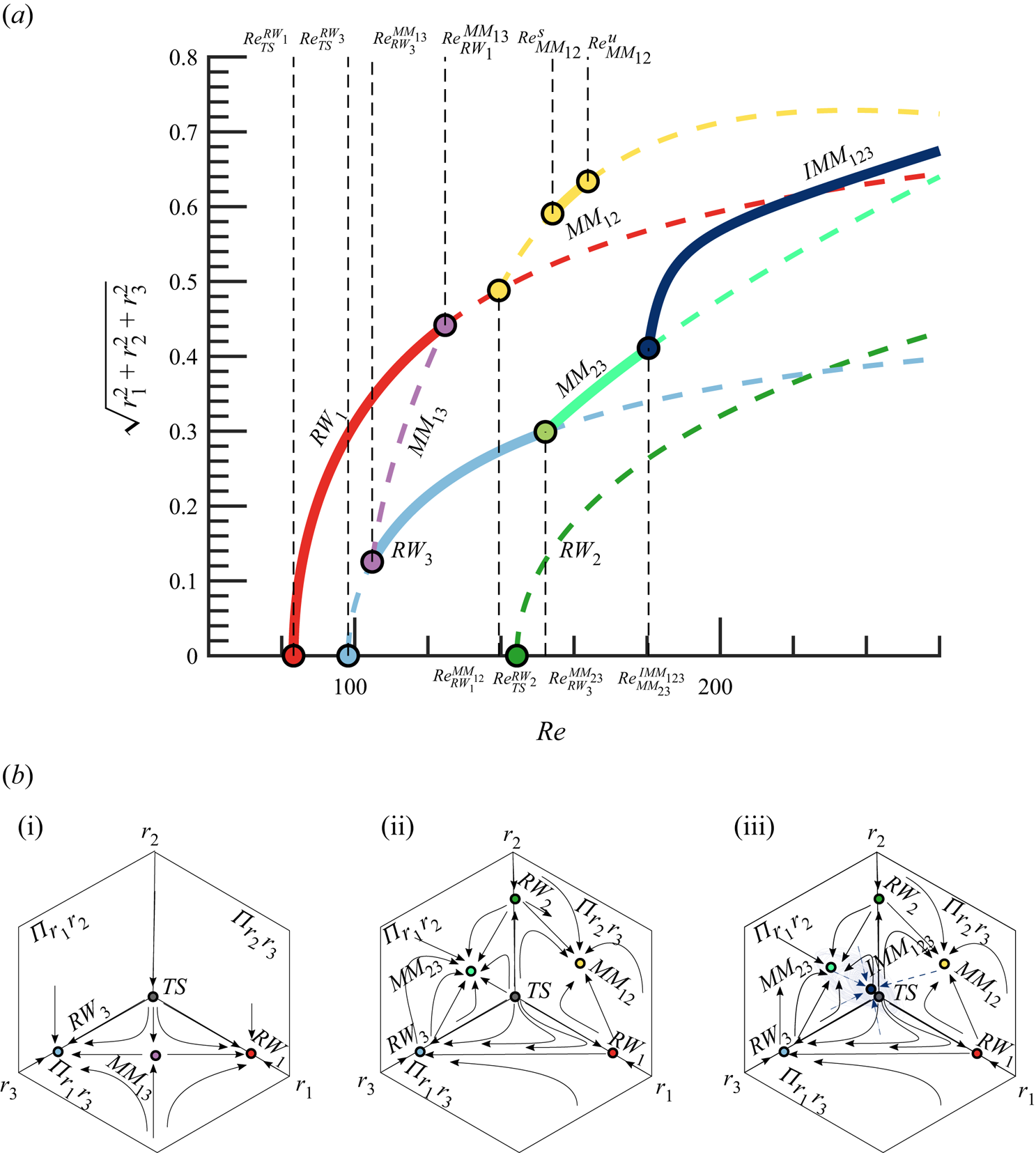
Figure 9. (a) Transition scenario at  ${{\varOmega }} = 1.75$. Attractors are depicted with solid lines, whereas unstable invariant states are represented with dashed lines.(b) Schematic representation of phase portraits. (i) Two stable rotating waves separated by a mixed-mode solution. (ii) Two stable mixed modes. (iii) An interacting mixed-mode attractor, the chaotic attractor that shadows the $IMM_{123}$ is sketched in a lighter blue colour.
5. Bifurcation scenario
5.1. Comparison with DNS
In this section we assess the validity of the normal form to characterize the bifurcation scenario, as well as its capability to predict accurately the frequencies and force coefficients of the flow. The estimations of the normal form are compared with DNS results, which are performed at constant rotation rate  $\varOmega =1.75$, the scenario analysed in § 4.2. As a first guess, we show the accurate prediction of the fundamental frequencies of each of the invariant states from normal form analysis in figure 10(a) in comparison with DNS results (markers), which will be discussed below.
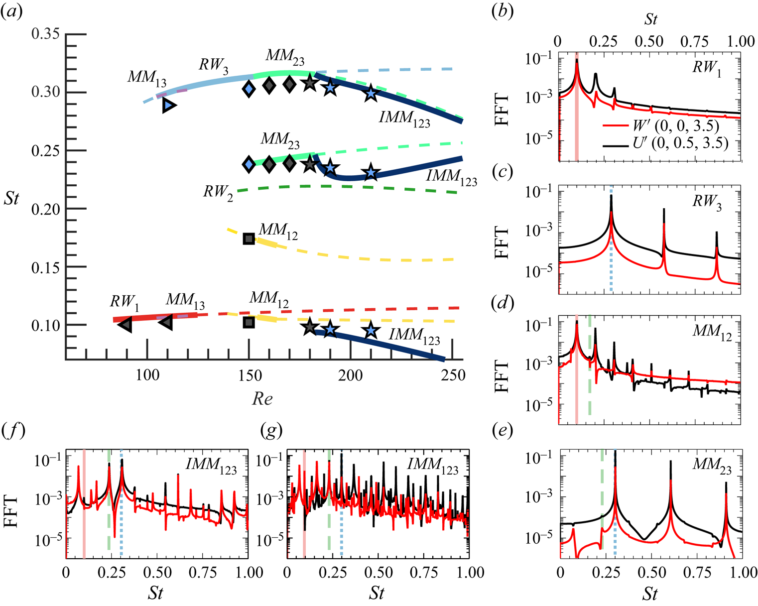
Figure 10. Frequency characterization of the flow at  $\varOmega = 1.75$. (a) Frequency evolution estimated from the normal form (continuous lines), where attractors are represented with continuous lines, whereas unstable invariant solutions are depicted with dashed lines. The markers of figure (a) denote the resulting pattern obtained from a time-stepping simulation; axisymmetric steady state $\circ$, $RW_1$ $\vartriangleleft$, $RW_3$ $\vartriangleright$, $MM_{12}$ $\square$, $MM_{23}$ $\lozenge$, IMM 123 $\star$, the family of initial conditions is visualized by colours (family I: grey, family II: blue). Figures (b–g) display the FFT fluctuating velocity spectra for the different regimes obtained by means of DNS. Two velocity components: $W'$ (red solid line), $U'$ (black solid line) and locations (0, 0, 3.5) and (0, 0.5, 3.5), respectively, are selected to characterize all the frequencies in the wake. Unstable mode frequencies are included: low frequency (light red solid line), medium frequency (light green dashed line) and high frequency (light blue dotted line). Results are shown for (b) $Re = 110$, (c) $Re = 110$, (d) $Re = 150$, (e) $Re = 150$, ( f) $Re = 181$, (g) $Re = 210$.
Direct numerical simulations have been carried out to confirm the existence of the bi-stability of full governing equations (2.1) at  $Re=110$. In particular, two families of time-stepping simulations have been performed with two distinct initial conditions, in such a way that, after a transient period, each of them converged towards different time-periodic solutions. On the one hand, we have used a static, axisymmetric base flow initially obtained at $Re = 70$, $\varOmega = 0$ which is able to develop the $RW_{1}$ state (family I, grey markers). On the other hand, we have used the solution obtained by Lorite-Díez & Jiménez-González (Reference Lorite-Díez and Jiménez-González2020) at $Re = 250$, $\varOmega = 2.2$ as initial seed to find the $RW_{3}$ state (family II, blue markers), which in turn confirms the existence of multiple stable attractors at $Re = 110$.
To determine the observed regimes, we have computed the frequency components corresponding to  $St_{RW_1}$ and $St_{RW_3}$, displayed in figure 10(b,c), using fast Fourier transform (FFT) spectra of pointwise streamwise and radial velocities in the near wake. The spectra are calculated using the oscillatory part of the velocity-time evolution, i.e. $U' = U-\bar {U}$ for the radial velocity component, where $\bar {\cdot }$ stands for the temporal averaging operator. The three-dimensional topology of the two rotating wave patterns are displayed by means of iso-surfaces of $Q$ quantity in figure 11, where single and double helices topologies are shown.
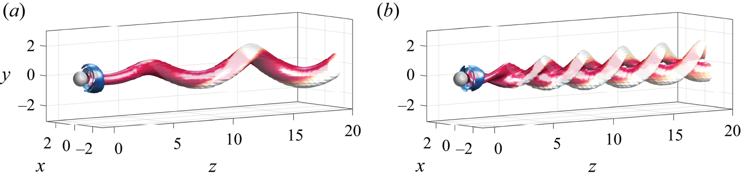
Figure 11. Three-dimensional structures of  $RW_1$ (a) and $RW_3$ (b) at $Re=110$ and $\varOmega =1.75$. We have used isosurfaces of Q-criterion, $Q=0.001$, coloured by streamwise vorticity, $\varpi _{z} \in [-1,1]$ (blue to red) to depict the flow structure.
Similarly, the existence of two stable mixed-mode attractors ( $MM_{12}$ and $MM_{23}$) is confirmed at $Re=150$. Two time-stepping simulations of the full governing equations at $\mbox { {Re}} = 150$ were performed, using $RW_{1}$ and $RW_{3}$ solutions as initial seeds, the resulting frequency spectra of these patterns are displayed in figure 10(d,e), where the different frequencies associated with $MM_{12}$ and $MM_{23}$ are identified. In particular, we can see that the appearance of the medium-frequency component originates quasiperiodic regimes. The mixed mode $MM_{12}$ has been detected only in a small interval of Reynolds numbers, which is faithfully captured by the normal form; however, the value of $Re^{s}_{MM_{12}} \approx 154$ slightly differs from the results of the DNS, which show a stable $MM_{12}$ for $Re=150$. The corresponding patterns are displayed in figure 12(a,b).
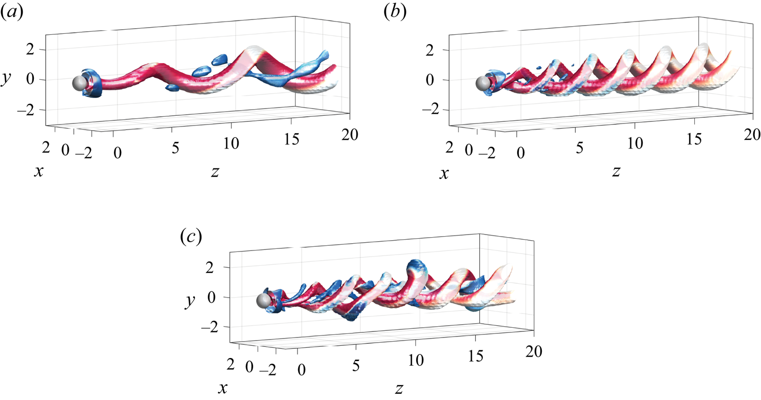
Figure 12. Three-dimensional structure of  $MM_{12}$ (a), $MM_{23}$ (b) and $IMM_{123}$ (c) at $Re=150$ (a,b) and $Re=210$ (c) and $\varOmega =1.75$. We have used isosurfaces of Q-criterion, $Q=0.001$, coloured by streamwise vorticity, $\varpi _{z} \in [-1,1]$ (blue to red) to depict the flow structure.
The  $T^{3}$-quasiperiodic state $IMM_{123}$ has been detected with DNS for Reynolds numbers $Re \approx 181$. Such a state seems to be the single stable attractor in the analysed range $181 < Re < 210$. A series of DNS were carried out with two families of initial conditions: the mixed modes $MM_{12}$ and $MM_{23}$, both obtained at lower Reynolds numbers. Eventually, every DNS converged to the $IMM_{123}$ state, which seems to confirm the claim that it is the single stable attractor. Their associated spectra is depicted in figure 10( f,g) and its complex topology can be seen in figure 12(c). The identification of the three main frequencies (low, medium and high) in the spectra, figure 10( f), along with the multiple nonlinear interactions between them is possible for Reynolds number values near the bifurcation value $Re^{IMM_{123}}_{MM_{23}}\simeq 181$. However, it rapidly departs from the $T^{3}$-quasiperiodic state towards a more irregular state ( $Re=210$) with a nearly continuous velocity spectrum, depicted in figure 10(g).
Globally, the good agreement between normal form analysis and DNS frequencies shows the predictive capability of the normal form within the range of Reynolds numbers studied (see figure 10a).
A further investigation of the dynamics of this attractor has been carried out by means of the  $0-1$ test. Such a test was introduced by Gottwald & Melbourne (Reference Gottwald and Melbourne2004, Reference Gottwald and Melbourne2009) to distinguish between regular and chaotic dynamics. More precisely, it corresponds to a dichotomy test where an estimate $K$, associated to an asymptotic growth of the dynamics, takes discrete values $[0,1]$ which are associated with non-chaotic ( $0$) and chaotic ( $1$). Further details are given in Appendix F. The results corresponding to the application of the test to the local radial velocity $U'(0,0.5,3.5)$, obtained for the two families of computations, indicate a rapid departure towards chaotic dynamics, displayed in the Appendix (figure 16). These results confirm that the transition scenario is eventually ended by the Newhouse–Takens–Ruelle route to chaos.
Furthermore, DNS results can be used to illustrate the spatial pattern associated with each fundamental frequency (low, medium, high). To that aim, a high-order dynamic mode decomposition (HODMD) technique (see Vega & Le Clainche Reference Vega and Le Clainche2020, and references therein) has been applied to instantaneous fields of streamwise vorticity  $\varpi _z$ located at $z = 2.5$ to isolate the spatial distributions of the main frequency components. More details about the HODMD technique and its application to present data can be found in Appendix E. In particular, the application of the technique to flow patterns $MM_{12}$, $MM_{23}$ and $IMM_{123}$ allowed the spatial characterization of the fundamental frequencies and their interactions. Apart from these frequencies, the methodology also provides the approximate contribution of each fundamental mode in the nonlinear state. The spatial patterns identified by HODMD are depicted using contours of spanwise vorticity without normalization. Thus, for the $MM_{12}$ state, the HODMD decomposition identifies four energetic modal contributions, corresponding to frequencies $St=0, 0.103, 0.174$ and $0.072$, which are depicted in figure 13(a). The use of instantaneous snapshots of $\varpi _z$ allows identifying mean flow ( $St=0$) given by the constant streamwise rotation. Likewise, the low-frequency component ( $St=0.103$) displays a dipole $m=-1$ topology. Similarly, the medium-frequency component ( $St=0.174$), also features a $m=-1$ structure, although their topology resembles the Yin-Yang mode (Auguste, Fabre & Magnaudet Reference Auguste, Fabre and Magnaudet2010). Finally, an axisymmetric $m=0$ topology is identified at $St=0.072$, as the product of the interaction between low-frequency (LF) and medium-frequency (MF) modes, $St_{m_0} \simeq St_{MF}-St_{LF}$. Such a mode is specially energetic close to the longitudinal axis and even dominant in some locations. In Lorite-Díez & Jiménez-González (Reference Lorite-Díez and Jiménez-González2020) the authors identified such a mode as a fundamental frequency of the flow, named $f_b$ therein. However, given the results from linear stability and normal form analysis, we have now identified this mode as a subproduct.

Figure 13. Nonlinear patterns identified through HODMD analysis. The patterns are depicted using streamwise vorticity contours,  $\varpi _z$. Results are shown for (a) $MM_{12}$, (b) $MM_{23}$ and (c) $IMM_{123}$ regimes. Tags values inside the contours refer to the corresponding frequency of each mode, $St_i$.
The same analysis for the  $MM_{23}$ regime allows the identification of three main frequency components, depicted in figure 13(b). Apart from the mean flow ( $St=0$), the flow decomposition pinpoints a mode with high frequency (HF) $St_{HF}=0.304$, that displays a $m=-2$ structure. In addition, the Yin-Yang mode is also retrieved but now with a frequency, $St_{MF}=0.238$. Note that, the amplitude associated with this medium-frequency component is very small. The weak energy associated with such a medium-frequency mode in the $MM_{23}$ regime is also observable in the corresponding spectra in figure 10(e).
Furthermore, the HODMD analysis of the complex regime  $IMM_{123}$, present at $Re= 210$ and $\varOmega =1.75$, is depicted in figure 13(c). The decomposition identifies the axisymmetric mean flow, the three fundamental frequencies and many interactions between them, although only five energetic components have been selected for depiction. For instance, the low-frequency and medium-frequency modes display $m=-1$ symmetries and respective frequencies $St_{LF}=0.095$ and $St_{MF}=0.231$, which are similar to those corresponding to the $MM_{12}$ and $MM_{23}$ regimes. Similarly, the frequency value of the high-frequency mode ( $m=-2$) remains nearly constant with respect to previous regimes, $St_{HF}=0.299$, indicating that the dependence of frequencies with $Re$ is small (as in figure 3b). Among the main subproducts, the axisymmetric pattern ( $m=0$) produced by the interaction of fundamental frequencies $St_{m0}\simeq St_{LF}+St_{HF}-St_{MF}=0.163$ stands out. It should be noted that there is a small mismatch between the identified peaks in FFT and the frequencies obtained by HODMD that is produced by the different sampling period and the corresponding recording frequency during the simulation.
To complement the previous analysis, we next focus on the effect of the different flow states, shown in figure 11 and figure 12, on the sphere's aerodynamic forces. Thus, we present in figure 14(a) the evolution with respect to Reynolds number at  $\varOmega =1.75$ of the time-averaged drag coefficient, $\overline {C_{D}}=\overline {C_{z}}$, and on figure 14(b) the total transverse force coefficient $\overline {C_L}=\overline {\sqrt {C^{2}_{x}+C^{2}_{y}}}$ for normal form analysis and DNS.
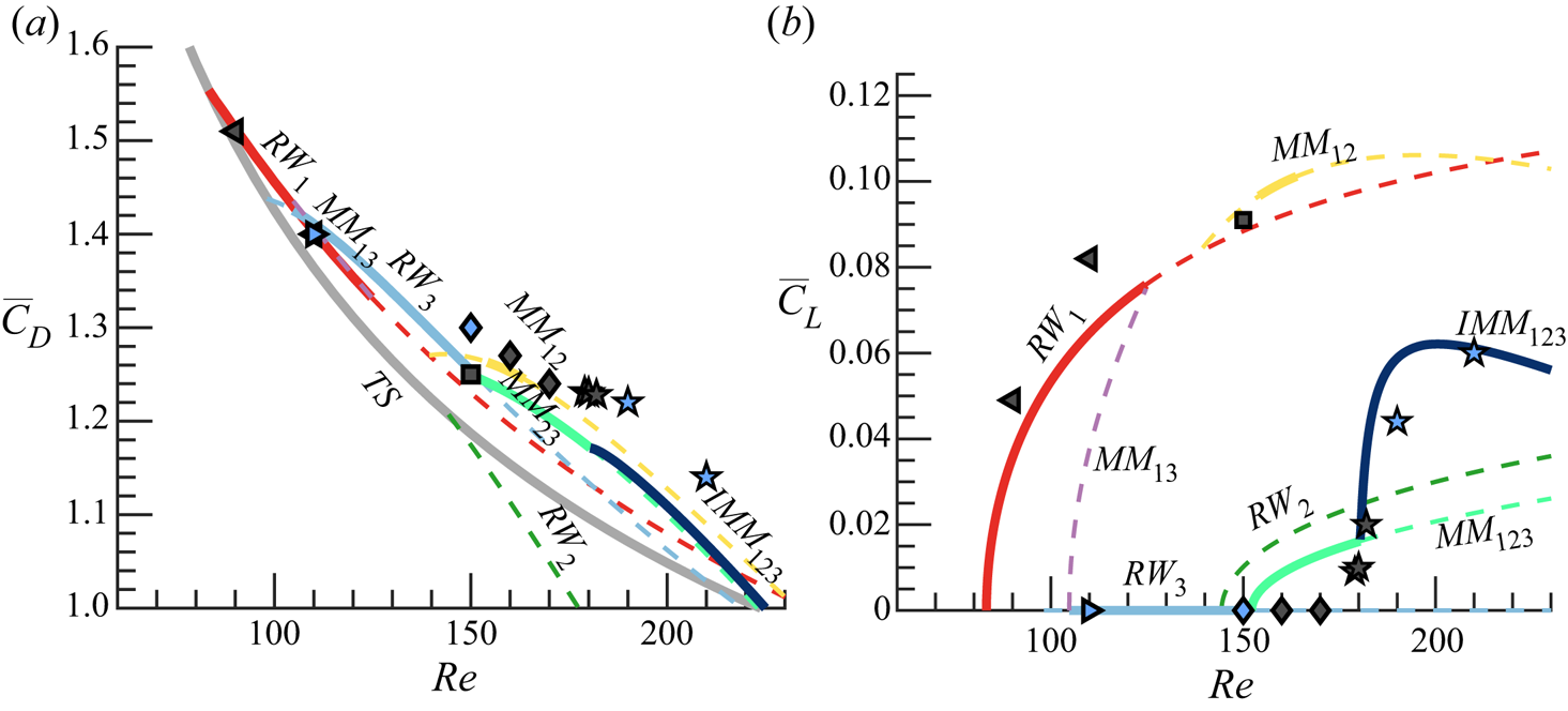
Figure 14. Evolution of the time-averaged forces with respect to Reynolds number for a constant rotation rate  $\varOmega =1.75$. The force coefficients determined from the normal form analysis are represented by continuous lines. The force coefficients determined from DNS are depicted with markers. Same legend as in figure 10.
The comparison between force coefficients obtained by means of normal form and DNS approaches is indeed fairly satisfactory. The method captures the main trends in the forces and, for most of the states, the prediction is reasonably similar, as it was with the different fundamental frequencies. More precisely, for simpler regimes, such as rotating waves, the normal form analysis and DNS provide the same results. At  $Re = 150$, for mixed modes, both methods display a small discrepancy (below five percent). This seems to be related to a small nonlinear contribution of the medium-frequency mode identified by the DNS, as it can be seen in the corresponding FFT spectra (see figure 10d,e). That said, the general trend of the mean drag $\overline {C_D}$ displays a general reduction with $Re$, which may be partly due to a smaller viscous drag contribution. Besides, the pressure drag component is likely to decrease as well, since $L_r$ is shown to increase with $Re$ (see figure 5b) for a given rotation rate, $\varOmega$. In particular, as discussed by Roshko (Reference Roshko1993) for three-dimensional bluff body wakes, an increase of the recirculating length leads to a decrease in the drag values on account of a pressure recovery associated to changes in the curvature of the separatrix line. Additionally, major changes in the trends are reported between different flow regimes, as expected from strong modifications in the near wake topology and flow separation (Lorite-Díez & Jiménez-González Reference Lorite-Díez and Jiménez-González2020).
Similarly, the agreement is also good for the mean total transverse coefficient,  $\overline {C_L}$, although it displays small deviations for states $RW_1$ and $MM_{23}$ (see figure 14b). The value of $\overline {C_L}$ is strongly affected by the wake regime and the corresponding azimuthal symmetry. Therefore, the two families of simulations display quite a different evolution. Moreover, it should be noted that the high-frequency mode does not create a net component of transverse force due their symmetric wake topology, as it is seen for $RW_{3}$ and $MM_{23}$ regimes, where this mode is dominant, causing $\overline {C_L}\simeq 0$. In those cases, the wake structures net eccentricity is small, inducing a negligible transverse force. In view of such results, such regimes should be favoured in case of control if a stabilization of the trajectory is wished, e.g. for freely rising or falling rotating spheres, as the transverse displacement of the body might be limited. Conversely, $RW_1$, $MM_{12}$ and $IMM_{123}$ are likely to cause lateral shift and destabilization of the trajectory for freely moving bodies due to their greater mean lateral force and their corresponding eccentric wake structures.
5.2. Parametric exploration
Let us discuss the influence of the rotation rate in the dynamics of the flow past the rotating sphere. For that purpose, we determine the stable attractors of the normal form in the range  $\mbox { {Re}} < 300$ and ${{\varOmega }} < 4$. The cubic normal form coefficients are determined following the same procedure as in § 4.2. However, for low rotation rates ( $\varOmega < 0.8$), we found that the linear coefficients of the normal form were not correctly estimated. So, for these values of the rotation rate, the linear coefficients are determined exactly at the threshold of instability of each codimension-one bifurcation.
The flow past the static sphere ( $\varOmega = 0$), analysed by Fabre et al. (Reference Fabre, Auguste and Magnaudet2008), experiences a symmetry breaking bifurcation that leads to the reflection-symmetric bifid wake (steady-state mode) and eventually a Hopf bifurcation that leads to the RSP. The phase diagram depicted in figure 15 shows that both the rotating wave $RW_1$ and the mixed mode $MM_{12}$ are the continuation in the parameter space of the steady-state and RSP mode, respectively. Thus, dynamics for low values of the rotation rate $(\varOmega < 1)$ are qualitatively similar to the flow past the static sphere. However, for rotation rate values slightly larger than $\varOmega _B$, one starts detecting a wake with a double helix. This fact has been evidenced by the numerical simulations of Lorite-Díez & Jiménez-González (Reference Lorite-Díez and Jiménez-González2020), Pier (Reference Pier2013) and the experimental work of Skarysz et al. (Reference Skarysz, Rokicki, Goujon-Durand and Wesfreid2018) who reported that at around ${{\varOmega }} \approx 1.5$ for large Reynolds numbers ( $Re > 250$) the quasiperiodic motion of the wake changes from a single to double helix pattern, which is consistent with the phase diagram in figure 15. However, if we look in detail at how the flow transits from a single helix to the double helix wake in terms of the rotation of the sphere, one can observe three bi-stable regions, between $RW_{1}$ and $RW_{3}$, between $RW_{3}$ and $MM_{12}$, and between $MM_{12}$ and $MM_{23}$. These bi-stable sections connect two regions of the parameter space with distinct attractors, the rotating waves $RW_{1}$ and $RW_{3}$ and the mixed modes $MM_{12}$ and $MM_{23}$. It is of interest that the formation of these new states occurs near the codimension-two point $B$, which exhibits the importance of this bifurcation as an organizing centre, even though it occurs as a bifurcation for an already unstable trivial state. Furthermore, the importance of the codimension point $A$ is clearly evidenced by figure 15, which also acts as an organizing centre of dynamics. Around point $A$, one finds four distinct regions with inequivalent dynamics. If we move counterclockwise from point $A$, we have the left region where the trivial axisymmetric state is stable, the lower region where the $RW_1$ state is the single attractor, a region with two stable attractors ( $RW_1$ and $RW_3$) and the upper region where the $RW_3$ is the single stable state. Finally, the significance of the other codimension-two bifurcation, the point $C$, is rather more subtle. This point is located in the only region where one can observe the mixed mode $MM_{13}$, which is only observed for very large rotation rates, and it connects the $RW_3$ state and the $T^{3}$-quasiperiodic state $IMM_{123}$.
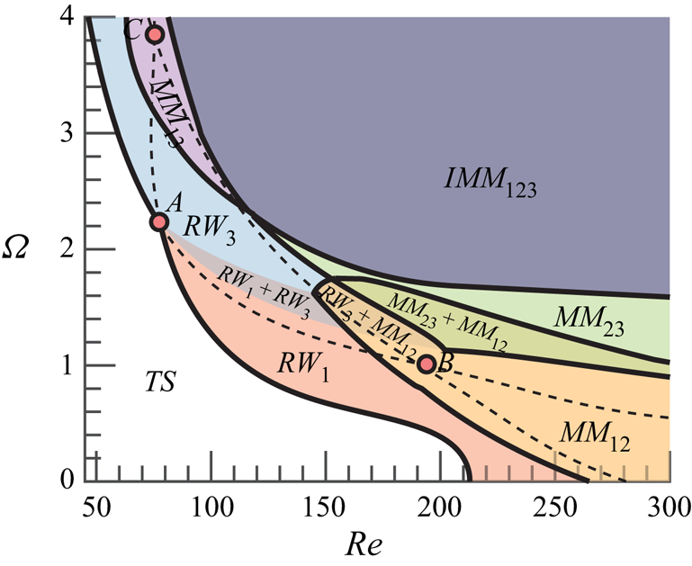
Figure 15. Phase diagram of the nonlinear patterns in the range  $\varOmega < 4$ and $\mbox { {Re}} < 300$, as predicted by the normal form (4.9). The axisymmetric state (TS) persists in the white region. Shaded regions indicate the existence of a stable pattern (respectively, stable patterns). Dashed lines illustrate unstable rotating waves neutral curves obtained by LSA.
Therefore, one may conclude that the rotation of the sphere has a mild effect on the bifurcation scenario for low rotation rates ( $\varOmega < 1$). Rotation rates between $1 < \varOmega < 2$ favourise the appearance of a double helix wake and hysteresic behaviour, whereas large rotation rates ( $\varOmega > 2$) have a destabilizing effect which rapidly triggers the emergence of chaotic dynamics via a Ruelle–Takens–Newhouse route.
6. Conclusion
The present study conducts a complete study of the transition scenario of the flow past a rotating sphere, which is a canonical model of many industrial and natural phenomena like particle-driven flows, sport aerodynamics, bubble motion, plant seeds, etc. In such applications the changes in the paths of the particles are related to the destabilization of complex flow regimes and associated force distributions. To gain a deeper understanding of the underlying physics and evaluate possibilities of flow and path control, we have studied the mode competition involved in the formation of patterns in the flow past a rotating sphere, associated sensitivity to forcing and the effect of flow regimes on the force coefficients. This research aimed to structurally study the pattern formation previously examined by Lorite-Díez & Jiménez-González (Reference Lorite-Díez and Jiménez-González2020), Pier (Reference Pier2013) and to determine from a dynamical perspective the fundamental building blocks of dynamics before and up to temporal chaos. In order to do that, we have employed LSA, normal form analysis and DNS.
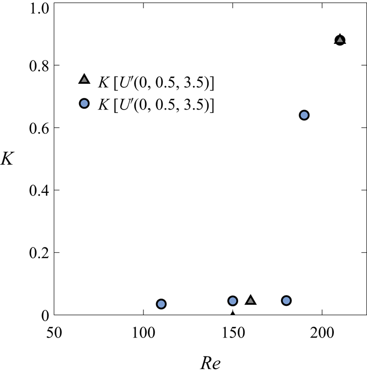
Figure 16. Asymptotic growth  $K$ associated with the local radial velocity $U'(0,0.5,3.5)$ (same as in figure 10). Results are shown for the different initial seeds: $RW_1$ (grey triangles) and $RW_3$ (blue circles).
Rotation of the sphere breaks the reflectional symmetry, thus inducing a preferential direction. This turns out to favourise the presence of rotating wave instabilities, instead of a steady symmetry breaking bifurcation, as it is the case for the flow past the static sphere. These instabilities exhibit a localized wavemaker within the recirculation zone, which is evidenced by the sensitivity maps. In addition, non-normality effects are weaker than in the flow past the static sphere, mainly because the primary bifurcation occurs at lower Reynolds number values. This might be an indication of a weaker transient growth of asymptotically stable perturbations for the rotating sphere wake flow (Chomaz Reference Chomaz2005).
The bifurcation scenario is qualitatively distinct and it greatly varies with the rotation rate, as it has been discussed in § 5.2. The flow field displays a large variety of attractors from rotating waves, quasiperiodic mixed modes to  $T^{3}$-quasiperiodic structures. In addition, one may find multiple attractors, which is associated to hysteresis, and it seems to be a common feature of many supercritical and subcritical flows, cf. (Subramanian, Sujith & Wahi Reference Subramanian, Sujith and Wahi2013; Guo et al. Reference Guo, Fauci, Shelley and Kanso2018; Ren et al. Reference Ren, Cheng, Xiong, Tong and Chen2021; Huang et al. Reference Huang, Ristroph, Luhar and Kanso2018; Suckale et al. Reference Suckale, Qin, Picchi, Keller and Battiato2018). Eventually, for sufficiently large Reynolds numbers, Lorite-Díez & Jiménez-González (Reference Lorite-Díez and Jiménez-González2020) and Pier (Reference Pier2013) identified irregular regimes for most rotation rates, which are associated to a $T^{3}$-quasiperiodic attractor. Nonetheless, such a state is just observed by means of DNS near its onset of existence. For larger Reynolds number values, the attractor is no longer quasiperiodic, but it is characterized by a continuous frequency spectra, that turns out to be chaotic. Indeed, such a chaotic attractor shadows the three frequency quasiperiodic state predicted by the normal form, which is evidenced by physical global features of the flow, e.g. the force acting on the surface of the sphere.
The analysis performed in this paper is able to accurately predict the fundamental modes of the wake flow, the bifurcation scenario and the forces acting on the sphere without the need of performing a fully nonlinear DNS. The results are compared against DNS computations at  $\varOmega =1.75$ with an excellent agreement in regime zones, mode frequencies and force coefficients. Then, our procedure has been validated without including non-normal and resonance effects in our analysis. In any case, their impact has been proven to be very reduced in this problem.
In the classification of the observed regimes, one may question which is the path or bifurcation scenario and how are they constituted, i.e. if it is possible to reconstitute the strange attractor with a sparse approximation. The identification of a  $T^{3}$-quasiperiodic state, complemented with DNS results, allows the justification that the route to chaos is indeed the Ruelle–Takens–Newhouse. This has several consequences for further studies of this or similar flows. First, we have been able to identify the route to chaos and the fundamental building blocks, which are the three rotating waves. One could attempt to obtain further insight into the chaotic attractor and to investigate physically interesting properties such as mixing or the forces on the sphere from the information extracted from the three unstable periodic orbits associated with the fundamental rotating waves. In this case, it seems reasonable to construct a symbolic alphabet with the main fundamental modes being the rotating waves. Then, one may approximate average quantities or the eigenvalues of the Perron–Frobenius operator by cycle expansions, cf. (Cvitanovic et al. Reference Cvitanovic, Artuso, Mainieri, Tanner, Vattay, Whelan and Wirzba2005), as it has been recently done by Yalnız & Budanur (Reference Yalnız and Budanur2020); Yalnız, Hof & Budanur (Reference Yalnız, Hof and Budanur2021) using algebraic topology techniques.
In addition, if ones attempt to design a control procedure to the quasiperiodic state or to prevent the presence of chaotic dynamics, the use of harmonic forcing, as in Sipp (Reference Sipp2012), seems a promising option, and the implementation is straightforward from the information provided in §§ 4 and 5. Additionally, the sensitivity to base flow modifications and structural sensitivity have been presented for the low-frequency and high-frequency modes in § 3.4 to analyse harmonic and steady control possibilities. It has been shown that the low-frequency mode displays a strong sensitivity inside the recirculating region, suggesting a higher receptivity to control through surface rear blowing, in line with the results presented in Niazmand & Renksizbulut (Reference Niazmand and Renksizbulut2005). In principle, the attenuation of the amplitude of such a mode would imply a decrease in the mean drag and total lift coefficients (see figure 14), which could presumably prevent the path's instability in the case of freely rising bodies, as those analysed by Mathai et al. (Reference Mathai, Zhu, Sun and Lohse2018). Therein, the tuning of rotational inertia is proposed to modify the wake and path's instabilities. The effect of changes in the moment of inertia may imply variations of the rotation rate, and consequently, changes in the regimes and associated forces. At that point, the force diagrams presented in figure 14 could be useful to guide such a tuning procedure and selectively set the regime of interest.
Acknowledgements
The authors are grateful to A. Chatterjee for useful discussions and the critical reading of the manuscript.
Funding
This work has been partially financed by the Junta de Andalucía, Universidad de Jaén, and European Funds under Project FEDER-UJA 1262764.
Declaration of interests
The authors report no conflict of interest.
Appendix A. Normal form reduction procedure for the triple-Hopf interaction
Before we detail the procedure for the reduction of the governing equations to the normal form (4.6), let us detail the terms that composed the compact notation of the governing equations (2.3), which is reminded here for the sake of conciseness,
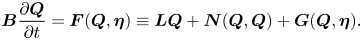 \begin{equation} \boldsymbol{B} \frac{\partial \boldsymbol{Q}}{\partial t} = \boldsymbol{F}(\boldsymbol{Q}, \boldsymbol{\eta}) \equiv \boldsymbol{L} \boldsymbol{Q} + \boldsymbol{N}(\boldsymbol{Q},\boldsymbol{Q}) + \boldsymbol{G} (\boldsymbol{Q},\boldsymbol{\eta}). \end{equation}
The operator  $\boldsymbol {G}(\boldsymbol {Q},\boldsymbol {\eta }) = \boldsymbol {G}(\boldsymbol {Q},[\eta _1,0]^\textrm {T}) + \boldsymbol {G}(\boldsymbol {Q},[0,\eta _2]^\textrm {T})$, where $\boldsymbol {G}(\boldsymbol {Q},[\eta _1,0]^\textrm {T}) = \eta _1 \boldsymbol {\nabla } \boldsymbol {\cdot } (\boldsymbol {\nabla } \boldsymbol {U} + \boldsymbol {\nabla } \boldsymbol {U}^\textrm {T})$ and $\boldsymbol {G}(\boldsymbol {Q},[0,\eta _2]^\textrm {T})$ expresses the imposition of the boundary condition $\boldsymbol {U} = (0, \eta _2, 0) \textrm { on } \varSigma _b$. The nonlinear operator $\boldsymbol {N}(\boldsymbol {Q}_1,\boldsymbol {Q}_2) = \boldsymbol {U}_1 \boldsymbol {\cdot } \boldsymbol {\nabla } \boldsymbol {U}_2$, and the linear operator accounts for the remaining terms that are linear on the state variable $\boldsymbol {Q}$, i.e. $\boldsymbol {L} \boldsymbol {Q} = [\boldsymbol {\nabla } P, \boldsymbol {\nabla } \boldsymbol {\cdot } \boldsymbol {U} ]^\textrm {T}$. In addition, we consider the following splitting of the parameters $\boldsymbol {\eta } = \boldsymbol {\eta }_c + \Delta \boldsymbol {\eta }$, where $\boldsymbol {\eta }_c$ denotes the critical parameters $\boldsymbol {\eta }_c \equiv [Re_c^{-1}, {{\varOmega }}_c]^\textrm {T}$ attained when the spectra of the Jacobian operator of the steady state posses at least an eigenvalue whose real part is zero, and $\Delta \boldsymbol {\eta } = [Re_c^{-1} - Re^{-1}, \varOmega _c - \varOmega ]^\textrm {T}$ the departure from the critical condition.
The procedure followed in this manuscript consists of the determination of a fifth-order Taylor expansion of the centre manifold, also known as the normal form, of the three codimension-two-Hopf points ( $A$,
$A$,  $B$,
$B$,  $C$), which enables a linear approximation of the cubic coefficients $\nu _{k \ell }$ and a quadratic approximation of the linear coefficients $\lambda _{\ell }$. The ultimate goal of this approach is the determination of the coefficients listed in tables 4–6. That is, to determine the cubic coefficient $\nu _{k \ell }$ values as
 \begin{equation} \nu_{k \ell} = \nu_{k \ell}^{(0)} + \varepsilon_{\nu}^{2} \nu_{k \ell}^{(\varepsilon_{\nu}^{2})} + \varepsilon^{2}_{{{\varOmega}}} \nu_{k \ell}^{(\varepsilon_{{{\varOmega}}}^{2})}, \end{equation}
where  $\nu _{k \ell }^{(0)},\nu _{k \ell }^{(\varepsilon _{\nu }^{2})}$ and $\nu _{k \ell }^{(\varepsilon _{{{\varOmega }}}^{2})}$ are determined at the two-Hopf point between mode $k$ and $\ell$. Similarly, the estimation of the linear coefficient is
 \begin{equation} \lambda_{\ell} = \varepsilon_{\nu}^{2} \lambda_{\ell}^{(\varepsilon_{\nu}^{2})} + \varepsilon_{{{\varOmega}}}^{2} \lambda_{\ell}^{(\varepsilon_{{{\varOmega}}}^{2})} + \varepsilon_{\nu}^{4} \lambda_{\ell}^{(\varepsilon_{\nu}^{4})} + \varepsilon_{{{\varOmega}}}^{4} \lambda_{\ell}^{(\varepsilon_{{{\varOmega}}}^{4})} + \varepsilon_{{{\varOmega}}}^{2}\varepsilon_{\nu}^{2} \lambda_{\ell}^{(\varepsilon_{\nu}^{2} \varepsilon_{{{\varOmega}}}^{2})}. \end{equation}
 The reduction to the normal form is carried out via a multiple scales expansion of the solution  $\boldsymbol {Q}$ of (2.3). The expansion considers a two-scale expansion of the original time, a fast time scale $t$ of the self-sustained instability and a slow time scale of the evolution of the amplitudes
 \begin{equation} t \mapsto t + \varepsilon^{2} \tau, \quad \varepsilon \ll 1, \end{equation}
here  $\varepsilon$ is the order of magnitude of the flow disturbances. The small parameters are
 \begin{equation} \varepsilon_{{{\varOmega}}}^{2} = \left({{\varOmega}}_c - {{\varOmega}} \right) \sim \varepsilon^{2} \quad \text{and}\quad \varepsilon_{\nu}^{2} = \left( \nu_c - \nu \right) = \left( \mbox{{Re}}_c^{{-}1} - \mbox{{Re}}^{{-}1} \right) \sim \varepsilon^{2}. \end{equation}
The ansatz of the expansion is
 \begin{equation} \displaystyle \boldsymbol{Q}(t,\tau) = \boldsymbol{Q}_b + \varepsilon \boldsymbol{q}_{(\varepsilon)}(t,\tau) + \varepsilon^{2} \boldsymbol{q}_{(\varepsilon^{2})}(t,\tau) + \varepsilon^{3} \boldsymbol{q}_{(\varepsilon^{3})}(t,\tau) + \varepsilon^{4} \boldsymbol{q}_{(\varepsilon^{4})}(t,\tau) + O(\varepsilon^{5}). \end{equation}
Note that the expansion of the left-hand side of (2.3) up to fifth order is
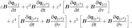 \begin{align} & \displaystyle \varepsilon \boldsymbol{B} \frac{\partial \boldsymbol{q}_{(\varepsilon)}} {\partial t} + \varepsilon^{2} \boldsymbol{B} \frac{\partial \boldsymbol{q}_{(\varepsilon^{2})}} {\partial t} + \varepsilon^{3} \left[ \boldsymbol{B} \frac{\partial \boldsymbol{q}_{(\varepsilon^{3})}} {\partial t} + \boldsymbol{B} \frac{\partial \boldsymbol{q}_{(\varepsilon)}} {\partial \tau} \right]\nonumber\\ &\quad + \displaystyle \varepsilon^{4} \left[ \boldsymbol{B} \frac{\partial \boldsymbol{q}_{(\varepsilon^{4})}} {\partial t} + \boldsymbol{B} \frac{\partial \boldsymbol{q}_{(\varepsilon^{2})}} {\partial \tau} \right] + \varepsilon^{5} \left[ \boldsymbol{B} \frac{\partial \boldsymbol{q}_{(\varepsilon^{5})}} {\partial t} + \boldsymbol{B} \frac{\partial \boldsymbol{q}_{(\varepsilon^{3})}} {\partial \tau} \right], \end{align}
respectively the right-hand side is
 \begin{equation} \boldsymbol{F} (\boldsymbol{q}, \boldsymbol{\eta}) = \boldsymbol{F}_{(0)} + \varepsilon \boldsymbol{F}_{(\varepsilon)} + \varepsilon^{2} \boldsymbol{F}_{(\varepsilon^{2})} + \varepsilon^{3} \boldsymbol{F}_{(\varepsilon^{3})} + \varepsilon^{4} \boldsymbol{F}_{(\varepsilon^{4})} + \varepsilon^{5} \boldsymbol{F}_{(\varepsilon^{5})}. \end{equation}
Then we are left with the determination of the forcing terms of (A8).
The reduction detailed in this appendix considers the interaction between two rotating wave solutions at a codimension-two point. In the following, we adopt the notation for the solutions  $z_1$ and $z_2$, which correspond to point $C$. In order to proceed for the other two points, replace $z_1$ by $z_3$ or $z_2$ by $z_3$.
A.1. Notation
Since the number of terms grows quickly with the order, in order to enhance readability, we define the set of vectors of linear, quadratic, cubic and fourth-order interactions as
 \begin{align} \boldsymbol{Z} &\equiv \{ z_1, z_2\}, \quad \overline{\boldsymbol{Z}} = \{ \bar{z}_1, \bar{z}_2 \}, \nonumber\\ \boldsymbol{Z}^{2} &\equiv \boldsymbol{Z} \otimes \boldsymbol{Z} \oplus \boldsymbol{Z} \otimes \overline{\boldsymbol{Z}} = \{ z_1^{2}, z_1 z_2, z_2^{2}, |z_1|^{2}, z_1 \bar{z}_2, |z_2|^{2} \}, \nonumber\\ \boldsymbol{Z}^{3} &\equiv \boldsymbol{Z} \otimes \boldsymbol{Z}^{2} \oplus \boldsymbol{Z}^{2} \otimes \overline{\boldsymbol{Z}} \nonumber\\ &= \{ z_1^{3}, z_1^{2} z_2, z_1 z_2^{2}, z_2^{3}, z_1 |z_1|^{2}, z_2 |z_1|^{2}, z_2^{2} \bar{z}_1, \bar{z}_2 z_1^{2}, z_1 |z_2|^{2}, z_2 |z_2|^{2} \}, \nonumber\\ \boldsymbol{Z}^{4} &\equiv \boldsymbol{Z}^{2} \otimes \boldsymbol{Z}^{2} \oplus \boldsymbol{Z} \otimes \overline{\boldsymbol{Z}}^{3} \nonumber\\ &= \{ z_1^{4}, z_1^{3} z_2, z_1^{2} z_2^{2}, z_1 z_2^{3}, z_2^{4}, z_1^{2} |z_1|^{2}, z_1 z_2 |z_1|^{2}, z_2^{2} |z_1|^{2}, z_1^{2} |z_2|^{2}, \nonumber\\ & \quad z_1 z_2 |z_2|^{2}, z_2^{2} |z_2|^{2}, z_1 \bar{z}_2 |z_1|^{2}, z_1 \bar{z}_2 |z_2|^{2}, z_1^{3} \bar{z}_2, \bar{z}_1 z_2^{3} \}, \end{align}
where only unique elements are kept. We denote by  $\boldsymbol {z}^{n}_\alpha$ any element of the family $\boldsymbol {Z}^{n}$, with $n \in \mathbb {N}^{*}$. In addition to these sets, we shall define the set of resonant terms
 \begin{equation} \boldsymbol{Z}_R \equiv \{ z_1, z_2, z_1 |z_1|^{2}, z_1 |z_2|^{2} \}. \end{equation}
A.2. Zeroth order
The zeroth order corresponds to the steady-state problem of the governing equations evaluated at the threshold of instability, i.e.  $\Delta \boldsymbol {\eta } = \boldsymbol {0}$,
 \begin{equation} \boldsymbol{0} = \boldsymbol{F} (\boldsymbol{Q}_b, \boldsymbol{0}), \end{equation}
whose solution is the steady state  $\boldsymbol {Q}_b$.
A.3. First order
The first order corresponds to the resolution of a homogeneous linear system, i.e. the generalized eigenvalue problem evaluated at the threshold of instability, i.e.  $\Delta \boldsymbol {\eta } = \boldsymbol {0}$. In such a case, the vector is expanded as
 \begin{equation} \boldsymbol{q}_{(\varepsilon)} = z_1 \hat{\boldsymbol{q}}_{(z_{1})} \exp({-\mathrm{i} (m_1 \theta + \omega_1 t)}) + z_2 \hat{\boldsymbol{q}}_{(z_{2})} \exp({-\mathrm{i} (m_2 \theta + \omega_2 t)}) + \text{c.c.} \end{equation}
Then, the eigenpairs  $[\mathrm {i} \omega _{\ell }, \hat {\boldsymbol {q}}_{(z_{\ell })} ]$ are determined as the solutions of the following eigenvalue problem:
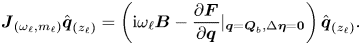 \begin{equation} \displaystyle \boldsymbol{J}_{(\omega_{\ell}, m_{\ell})} \hat{\boldsymbol{q}}_{(z_{\ell})} = \left( \mathrm{i} \omega_{\ell} \boldsymbol{B} - \frac{\partial \boldsymbol{F}}{\partial \boldsymbol{q} }|_{\boldsymbol{q} = \boldsymbol{Q}_b, \Delta \boldsymbol{\eta} = \boldsymbol{0}} \right) \hat{\boldsymbol{q}}_{(z_{\ell})}. \end{equation}
 The eigenmode  $\hat {\boldsymbol {q}}_{(z_{\ell })}(r,z)$ is then normalised in such a way that $\langle \boldsymbol {\hat u}_{({z}_{\ell })}, \boldsymbol {\hat u}_{({z}_{\ell })} \rangle _{L^{2}} = 1$.
A.4. Second order
The second-order expansion term  $\boldsymbol {q}_{(\varepsilon ^{2})}(t,\tau )$ is determined by the resolution of a set of linear systems, where the forcing terms are evaluated from first- and zeroth-order terms. The expansion in terms of amplitudes $z_{\ell }(\tau )$ of $\boldsymbol {q}_{(\varepsilon ^{2})}(t,\tau )$ is assessed by collecting the second-order forcing terms. Nonlinear second-order terms in $\varepsilon$ are
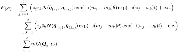 \begin{align} \displaystyle \boldsymbol{F}_{(\varepsilon^{2})} & \equiv \displaystyle \sum_{j,k=1}^{2} \left( z_j z_k \boldsymbol{N}(\hat{\boldsymbol{q}}_{(z_{j})},\hat{\boldsymbol{q}}_{(z_{k})}) \exp({-{\rm i}(m_j+m_k)\theta}) \exp({-{\rm i}(\omega_j+\omega_k)t}) + \text{c.c.} \right) \nonumber\\ &\quad + \displaystyle \sum_{j,k=1}^{2} \left( z_j \bar{z}_k \boldsymbol{N}(\hat{\boldsymbol{q}}_{(z_{j})},\hat{\boldsymbol{q}}_{(\bar{z}_{k})}) \exp({-{\rm i}(m_j-m_k)\theta}) \exp({-{\rm i}(\omega_j - \omega_k)t}) + \text{c.c.} \right) \nonumber\\ &\quad + \displaystyle \sum_{\ell=1}^{2} \eta_{\ell} \boldsymbol{G}(\boldsymbol{Q}_b, \boldsymbol{e}_{\ell}), \end{align}
where  $\boldsymbol {e}_{\ell }$ is an element of the orthonormal basis of $\mathbb {R}^{2}$. Then the second-order expansion of the flow variable is carried out so it matches the terms of the forcing (A14),
 \begin{equation} \boldsymbol{q}_{(\varepsilon^{2})} \equiv \displaystyle \sum_{\boldsymbol{z}_\alpha^{2} \in \boldsymbol{Z}} \left( \boldsymbol{z}^{2}_\alpha \hat{\boldsymbol{q}}_{(\boldsymbol{z}^{2}_\alpha)} \exp({-\mathrm{i} (m_\alpha \theta + \omega_\alpha t)}) + \text{c.c.} \right) + \displaystyle \sum_{\ell=1}^{2} \eta_{\ell} \boldsymbol{Q}_b^{(\eta_{\ell})}. \end{equation}
Terms  $\hat {\boldsymbol {q}}_{(z_j^{2})}$ are harmonics of the flow, $\hat {\boldsymbol {q}}_{(z_{j} z_{k})}$ with $j \neq k$ are coupling terms, $\hat {\boldsymbol {q}}_{(|z_j|^{2})}$ are harmonic base flow modification terms and $\boldsymbol {Q}_b^{(\eta _{\ell })}$ are base flow corrections due to a modification of the parameter $\eta _{\ell }$ from the critical point. Then the second-order terms are determined from the resolution of the following systems of equations:
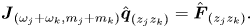 \begin{equation} \displaystyle \boldsymbol{J}_{(\omega_j + \omega_k, m_j + m_k)} \hat{\boldsymbol{q}}_{(z_{j} z_{k})} = \hat{\boldsymbol{F}}_{(z_j z_k)}. \end{equation}
Here  $\hat {\boldsymbol {F}}_{(z_j z_k)} \equiv \boldsymbol {N}(\hat {\boldsymbol {q}}_{(z_{j})},\hat {\boldsymbol {q}}_{(z_{k})}) + \boldsymbol {N}(\hat {\boldsymbol {q}}_{(z_{k})},\hat {\boldsymbol {q}}_{(z_{j})})$ and
 \begin{equation} \displaystyle \boldsymbol{J}_{(0,0)} \boldsymbol{Q}_b^{(\eta_{\ell})} = \boldsymbol{G}(\boldsymbol{Q}_b, \boldsymbol{e}_{\ell}). \end{equation}
A.5. Third order
At third order, we proceed as for previous orders, first the forcing term is expanded as
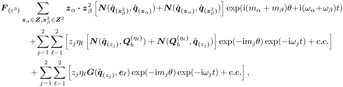 \begin{align}
\displaystyle {\boldsymbol{F}}_{(\varepsilon^{3})} &
\displaystyle \sum_{\boldsymbol{z}_\alpha \in
\boldsymbol{Z}, \boldsymbol{z}^{2}_\beta \in
\boldsymbol{Z}^{2} } \boldsymbol{z}_{\alpha}
\boldsymbol{\cdot} \boldsymbol{z}^{2}_{\beta} \left[
\boldsymbol{N}(\hat{\boldsymbol{q}}_{(\boldsymbol{z}^{2}_\beta)},
\hat{\boldsymbol{q}}_{(\boldsymbol{z}_{\alpha})}) \!+\!
\boldsymbol{N}(\hat{\boldsymbol{q}}_{(\boldsymbol{z}_\alpha)},
\hat{\boldsymbol{q}}_{(\boldsymbol{z}^{2}_\beta)}) \right]
\exp({\mathrm{i} (m_\alpha + m_\beta) \theta \!+\! \mathrm{i}
(\omega_\alpha \!+\! \omega_\beta) t}) \nonumber\\
&\quad \!+\! \displaystyle \sum_{\substack{j=1} }^{2}
\sum_{\substack{\ell=1} }^{2} \left[ z_j \eta_{\ell} \left[
\boldsymbol{N}(\hat{\boldsymbol{q}}_{(z_{j})},\boldsymbol{Q}_b^{(\eta_{\ell})})
+
\boldsymbol{N}(\boldsymbol{Q}_b^{(\eta_{\ell})},\hat{\boldsymbol{q}}_{(z_{j})})
\right] \exp({-{\rm i} m_j \theta}) \exp({-{\rm i} \omega_j
t}) + \text{c.c.} \right]\nonumber\\
&\quad + \displaystyle
\sum_{\substack{j=1} }^{2} \sum_{\substack{\ell=1} }^{2}
\left[ z_j \eta_{\ell}
\boldsymbol{G}(\hat{\boldsymbol{q}}_{(z_{j})},
\boldsymbol{e}_{\ell}) \exp({-{\rm i} m_j \theta})
\exp({-{\rm i} \omega_j t}) + \text{c.c.} \right],
\end{align}
\begin{align}
\displaystyle {\boldsymbol{F}}_{(\varepsilon^{3})} &
\displaystyle \sum_{\boldsymbol{z}_\alpha \in
\boldsymbol{Z}, \boldsymbol{z}^{2}_\beta \in
\boldsymbol{Z}^{2} } \boldsymbol{z}_{\alpha}
\boldsymbol{\cdot} \boldsymbol{z}^{2}_{\beta} \left[
\boldsymbol{N}(\hat{\boldsymbol{q}}_{(\boldsymbol{z}^{2}_\beta)},
\hat{\boldsymbol{q}}_{(\boldsymbol{z}_{\alpha})}) \!+\!
\boldsymbol{N}(\hat{\boldsymbol{q}}_{(\boldsymbol{z}_\alpha)},
\hat{\boldsymbol{q}}_{(\boldsymbol{z}^{2}_\beta)}) \right]
\exp({\mathrm{i} (m_\alpha + m_\beta) \theta \!+\! \mathrm{i}
(\omega_\alpha \!+\! \omega_\beta) t}) \nonumber\\
&\quad \!+\! \displaystyle \sum_{\substack{j=1} }^{2}
\sum_{\substack{\ell=1} }^{2} \left[ z_j \eta_{\ell} \left[
\boldsymbol{N}(\hat{\boldsymbol{q}}_{(z_{j})},\boldsymbol{Q}_b^{(\eta_{\ell})})
+
\boldsymbol{N}(\boldsymbol{Q}_b^{(\eta_{\ell})},\hat{\boldsymbol{q}}_{(z_{j})})
\right] \exp({-{\rm i} m_j \theta}) \exp({-{\rm i} \omega_j
t}) + \text{c.c.} \right]\nonumber\\
&\quad + \displaystyle
\sum_{\substack{j=1} }^{2} \sum_{\substack{\ell=1} }^{2}
\left[ z_j \eta_{\ell}
\boldsymbol{G}(\hat{\boldsymbol{q}}_{(z_{j})},
\boldsymbol{e}_{\ell}) \exp({-{\rm i} m_j \theta})
\exp({-{\rm i} \omega_j t}) + \text{c.c.} \right],
\end{align}
where  $\omega _n$ and $m_n$ are defined as $\omega _n = \omega _j + \omega _k + \omega _{\ell }$, $m_n = m_j + m_k + m_{\ell }$ with $n = j + k + \ell$. Followed by the expansion of the state variable $\boldsymbol {q}_{(\varepsilon ^{3})}(t,\tau )$,
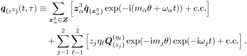 \begin{align} \displaystyle \boldsymbol{q}_{(\varepsilon^{3})}(t,\tau) & \equiv \displaystyle \sum_{\boldsymbol{z}_\alpha^{3} \in \boldsymbol{Z}} \left[ \boldsymbol{z}^{3}_\alpha \hat{\boldsymbol{q}}_{(\boldsymbol{z}^{3}_\alpha)} \exp({-\mathrm{i} (m_\alpha \theta + \omega_\alpha t)}) + \text{c.c.} \right]\nonumber\\ &\quad + \displaystyle \sum_{\substack{j=1} }^{2} \sum_{\substack{\ell=1} }^{2} \left[ z_j \eta_{\ell} \boldsymbol{Q}^{(\eta_{\ell})}_{(z_j)} \exp({-{\rm i} m_j \theta}) \exp({-{\rm i} \omega_j t}) + \text{c.c.} \right]. \end{align}
At this order there exist resonance terms, which are associated with the singular Jacobian  $\boldsymbol {J}_{(\omega _k,m_k)}$ for $k=1,2,3$. To ensure the solvability of these terms, we must enforce compatibility conditions, i.e. the Fredholm alternative. The resonant terms are then determined from the resolution of the following set of bordered systems:
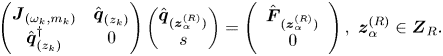 \begin{equation} \begin{pmatrix} \boldsymbol{J}_{(\omega_k,m_k)} & \hat{\boldsymbol{q}}_{(z_{k})} \\ \hat{\boldsymbol{q}}_{(z_{k})}^{{{{\dagger}}}} & 0 \end{pmatrix} \begin{pmatrix} \hat{\boldsymbol{q}}_{(\boldsymbol{z}^{(R)}_\alpha)} \\ s \end{pmatrix} = \left( \begin{array}{c} \hat{\boldsymbol{F}}_{(\boldsymbol{z}^{(R)}_\alpha)} \\ 0 \end{array} \right), \ \boldsymbol{z}^{(R)}_\alpha \in \boldsymbol{Z}_R. \end{equation}
Here  $s=\lambda ^{(\varepsilon _{\nu }^{2})}_k$ (respectively $s=\lambda ^{(\varepsilon _{{{\varOmega }}}^{2})}_k$) for $\boldsymbol {z}^{(R)}_\alpha =z_k$ and $s=\nu ^{(0)}_{kl}$ for $\boldsymbol {z}^{(R)}_\alpha = z_k |z_{\ell }|^{2}$. The non-resonant terms are then determined as at second order from the resolution of forced linear systems.
A.6. Fourth order
At fourth order we proceed as at second order, we expand the forcing term  $\boldsymbol {F}_{(\varepsilon ^{4})}$ as
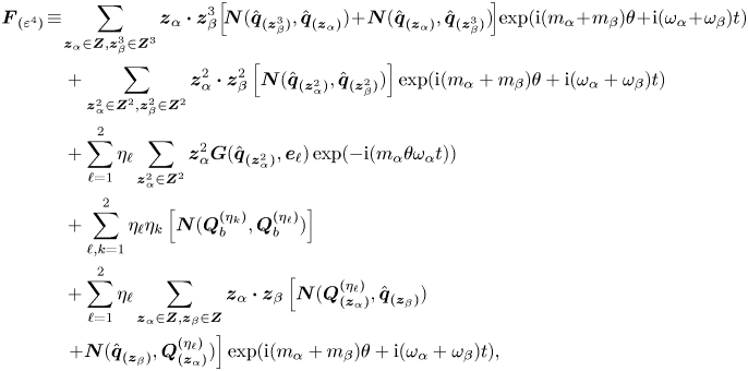 \begin{align}
\boldsymbol{F}_{(\varepsilon^{4})} &\!\equiv\! \displaystyle
\sum_{\boldsymbol{z}_\alpha \in \boldsymbol{Z},
\boldsymbol{z}^{3}_\beta \in \boldsymbol{Z}^{3} }
\boldsymbol{z}_{\alpha} \boldsymbol{\cdot}
\boldsymbol{z}^{3}_{\beta}\! \left[\!
\boldsymbol{N}(\hat{\boldsymbol{q}}_{(\boldsymbol{z}^{3}_\beta)},
\hat{\boldsymbol{q}}_{(\boldsymbol{z}_{\alpha})}) \!+\!
\boldsymbol{N}(\hat{\boldsymbol{q}}_{(\boldsymbol{z}_\alpha)},
\hat{\boldsymbol{q}}_{(\boldsymbol{z}^{3}_\beta)})\! \right]\!
\exp({\mathrm{i} (m_\alpha \!+\! m_\beta) \theta \!+\! \mathrm{i}
(\omega_\alpha \!+\! \omega_\beta) t})\nonumber\\
&\quad + \displaystyle \sum_{\boldsymbol{z}^{2}_\alpha \in
\boldsymbol{Z}^{2}, \boldsymbol{z}^{2}_\beta \in
\boldsymbol{Z}^{2} } \boldsymbol{z}^{2}_{\alpha}
\boldsymbol{\cdot} \boldsymbol{z}^{2}_{\beta} \left[
\boldsymbol{N}(\hat{\boldsymbol{q}}_{(\boldsymbol{z}^{2}_\alpha)},
\hat{\boldsymbol{q}}_{(\boldsymbol{z}^{2}_\beta)}) \right]
\exp({\mathrm{i} (m_\alpha + m_\beta) \theta + \mathrm{i}
(\omega_\alpha + \omega_\beta)t}) \nonumber\\ &\quad +
\displaystyle \sum_{\ell=1}^{2} \eta_{\ell}
\sum_{\boldsymbol{z}^{2}_\alpha \in \boldsymbol{Z}^{2}}
\boldsymbol{z}^{2}_\alpha
\boldsymbol{G}(\hat{\boldsymbol{q}}_{(\boldsymbol{z}^{2}_\alpha)},
\boldsymbol{e}_{\ell}) \exp({-\mathrm{i} (m_\alpha \theta
\omega_\alpha t)}) \nonumber\\ &\quad + \displaystyle
\sum_{\ell,k=1}^{2} \eta_{\ell} \eta_k
\left[\boldsymbol{N}(\boldsymbol{Q}_b^{(\eta_k)},\boldsymbol{Q}_b^{(\eta_{\ell})})
\right] \nonumber\\ &\quad + \displaystyle
\sum_{\ell=1}^{2} \eta_{\ell} \displaystyle
\sum_{\boldsymbol{z}_\alpha \in \boldsymbol{Z},
\boldsymbol{z}_\beta \in \boldsymbol{Z} }
\boldsymbol{z}_{\alpha} \boldsymbol{\cdot}
\boldsymbol{z}_{\beta} \left[
\boldsymbol{N}(\boldsymbol{Q}^{(\eta_{\ell})}_{(\boldsymbol{z}_\alpha)},
\hat{\boldsymbol{q}}_{(\boldsymbol{z}_\beta)})
\right.\nonumber\\ &\left. \quad +
\boldsymbol{N}(\hat{\boldsymbol{q}}_{(\boldsymbol{z}_\beta)},
\boldsymbol{Q}^{(\eta_{\ell})}_{(\boldsymbol{z}_\alpha)})
\right] \exp({\mathrm{i} (m_\alpha + m_\beta) \theta +
\mathrm{i} (\omega_\alpha + \omega_\beta) t}),
\end{align}
\begin{align}
\boldsymbol{F}_{(\varepsilon^{4})} &\!\equiv\! \displaystyle
\sum_{\boldsymbol{z}_\alpha \in \boldsymbol{Z},
\boldsymbol{z}^{3}_\beta \in \boldsymbol{Z}^{3} }
\boldsymbol{z}_{\alpha} \boldsymbol{\cdot}
\boldsymbol{z}^{3}_{\beta}\! \left[\!
\boldsymbol{N}(\hat{\boldsymbol{q}}_{(\boldsymbol{z}^{3}_\beta)},
\hat{\boldsymbol{q}}_{(\boldsymbol{z}_{\alpha})}) \!+\!
\boldsymbol{N}(\hat{\boldsymbol{q}}_{(\boldsymbol{z}_\alpha)},
\hat{\boldsymbol{q}}_{(\boldsymbol{z}^{3}_\beta)})\! \right]\!
\exp({\mathrm{i} (m_\alpha \!+\! m_\beta) \theta \!+\! \mathrm{i}
(\omega_\alpha \!+\! \omega_\beta) t})\nonumber\\
&\quad + \displaystyle \sum_{\boldsymbol{z}^{2}_\alpha \in
\boldsymbol{Z}^{2}, \boldsymbol{z}^{2}_\beta \in
\boldsymbol{Z}^{2} } \boldsymbol{z}^{2}_{\alpha}
\boldsymbol{\cdot} \boldsymbol{z}^{2}_{\beta} \left[
\boldsymbol{N}(\hat{\boldsymbol{q}}_{(\boldsymbol{z}^{2}_\alpha)},
\hat{\boldsymbol{q}}_{(\boldsymbol{z}^{2}_\beta)}) \right]
\exp({\mathrm{i} (m_\alpha + m_\beta) \theta + \mathrm{i}
(\omega_\alpha + \omega_\beta)t}) \nonumber\\ &\quad +
\displaystyle \sum_{\ell=1}^{2} \eta_{\ell}
\sum_{\boldsymbol{z}^{2}_\alpha \in \boldsymbol{Z}^{2}}
\boldsymbol{z}^{2}_\alpha
\boldsymbol{G}(\hat{\boldsymbol{q}}_{(\boldsymbol{z}^{2}_\alpha)},
\boldsymbol{e}_{\ell}) \exp({-\mathrm{i} (m_\alpha \theta
\omega_\alpha t)}) \nonumber\\ &\quad + \displaystyle
\sum_{\ell,k=1}^{2} \eta_{\ell} \eta_k
\left[\boldsymbol{N}(\boldsymbol{Q}_b^{(\eta_k)},\boldsymbol{Q}_b^{(\eta_{\ell})})
\right] \nonumber\\ &\quad + \displaystyle
\sum_{\ell=1}^{2} \eta_{\ell} \displaystyle
\sum_{\boldsymbol{z}_\alpha \in \boldsymbol{Z},
\boldsymbol{z}_\beta \in \boldsymbol{Z} }
\boldsymbol{z}_{\alpha} \boldsymbol{\cdot}
\boldsymbol{z}_{\beta} \left[
\boldsymbol{N}(\boldsymbol{Q}^{(\eta_{\ell})}_{(\boldsymbol{z}_\alpha)},
\hat{\boldsymbol{q}}_{(\boldsymbol{z}_\beta)})
\right.\nonumber\\ &\left. \quad +
\boldsymbol{N}(\hat{\boldsymbol{q}}_{(\boldsymbol{z}_\beta)},
\boldsymbol{Q}^{(\eta_{\ell})}_{(\boldsymbol{z}_\alpha)})
\right] \exp({\mathrm{i} (m_\alpha + m_\beta) \theta +
\mathrm{i} (\omega_\alpha + \omega_\beta) t}),
\end{align}
and the state variable  $\boldsymbol {q}_{(\varepsilon ^{4})}$ as
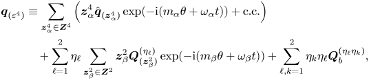 \begin{align} \boldsymbol{q}_{(\varepsilon^{4})} &\equiv \displaystyle \sum_{\boldsymbol{z}^{4}_\alpha \in \boldsymbol{Z}^{4}} \left( \boldsymbol{z}^{4}_\alpha \hat{\boldsymbol{q}}_{(\boldsymbol{z}^{4}_\alpha)} \exp({-\mathrm{i} (m_\alpha \theta + \omega_\alpha t)}) + \text{c.c.} \right)\nonumber\\ &\quad + \displaystyle \sum_{\ell=1}^{2} \eta_{\ell} \displaystyle \sum_{\boldsymbol{z}^{2}_\beta \in \boldsymbol{Z}^{2}} \boldsymbol{z}^{2}_\beta \boldsymbol{Q}^{(\eta_{\ell})}_{(\boldsymbol{z}^{2}_\beta)} \exp({-\mathrm{i} (m_\beta \theta + \omega_\beta t)}) + \sum_{\ell,k=1}^{2} \eta_k \eta_{\ell} \boldsymbol{Q}^{(\eta_{\ell} \eta_k)}_{b}, \end{align}
which are determined from the resolution of a forced linear system.
A.7. Fifth order
At fifth order, we uniquely consider the resonant terms. These are the coefficients of members of  $\boldsymbol {Z}_R$. The resonant forcing terms are
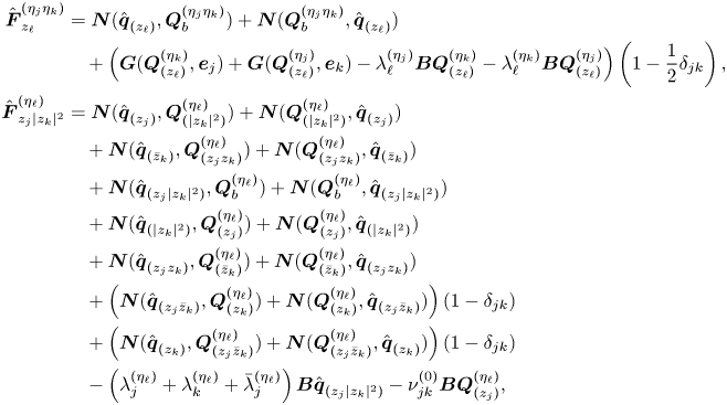 \begin{align} \hat{\boldsymbol{F}}^{(\eta_j \eta_k)}_{z_{\ell}} &= \boldsymbol{N}(\hat{\boldsymbol{q}}_{(z_{\ell})},\boldsymbol{Q}^{(\eta_j \eta_k)}_{b}) + \boldsymbol{N}(\boldsymbol{Q}^{(\eta_j \eta_k)}_{b},\hat{\boldsymbol{q}}_{(z_{\ell})}) \nonumber\\ & \quad + \left(\boldsymbol{G}( \boldsymbol{Q}^{(\eta_k)}_{(z_{\ell})}, \boldsymbol{e}_j) + \boldsymbol{G}(\boldsymbol{Q}^{(\eta_j)}_{(z_{\ell})}, \boldsymbol{e}_k ) - \lambda_{\ell}^{(\eta_j)} \boldsymbol{B} \boldsymbol{Q}^{(\eta_k)}_{(z_{\ell})} - \lambda_{\ell}^{(\eta_k)} \boldsymbol{B} \boldsymbol{Q}^{(\eta_j)}_{(z_{\ell})}\right) \left(1 - \frac{1}{2} \delta_{jk}\right), \nonumber\\ \hat{\boldsymbol{F}}^{(\eta_{\ell})}_{z_j |z_k|^{2}} &= \boldsymbol{N}(\hat{\boldsymbol{q}}_{(z_{j})},\boldsymbol{Q}^{(\eta_{\ell})}_{(|z_k|^{2})}) + \boldsymbol{N}(\boldsymbol{Q}^{(\eta_{\ell})}_{(|z_k|^{2})},\hat{\boldsymbol{q}}_{(z_{j})}) \nonumber\\ & \quad + \boldsymbol{N}(\hat{\boldsymbol{q}}_{(\bar{z}_{k})},\boldsymbol{Q}^{(\eta_{\ell})}_{(z_j z_k)}) + \boldsymbol{N}(\boldsymbol{Q}^{(\eta_{\ell})}_{(z_j z_k)},\hat{\boldsymbol{q}}_{(\bar{z}_{k})}) \nonumber\\ & \quad + \boldsymbol{N}(\hat{\boldsymbol{q}}_{(z_j |z_k|^{2})},\boldsymbol{Q}^{(\eta_{\ell})}_{b}) + \boldsymbol{N}(\boldsymbol{Q}^{(\eta_{\ell})}_{b},\hat{\boldsymbol{q}}_{(z_j |z_k|^{2})}) \nonumber\\ & \quad + \boldsymbol{N}(\hat{\boldsymbol{q}}_{(|z_k|^{2})},\boldsymbol{Q}^{(\eta_{\ell})}_{(z_j)}) + \boldsymbol{N}(\boldsymbol{Q}^{(\eta_{\ell})}_{(z_j)},\hat{\boldsymbol{q}}_{(|z_k|^{2})}) \nonumber\\ & \quad + \boldsymbol{N}(\hat{\boldsymbol{q}}_{(z_j z_k)},\boldsymbol{Q}^{(\eta_{\ell})}_{(\bar{z}_k)}) + \boldsymbol{N}(\boldsymbol{Q}^{(\eta_{\ell})}_{(\bar{z}_k)},\hat{\boldsymbol{q}}_{(z_j z_k)}) \nonumber\\ & \quad + \left(\boldsymbol{N}(\hat{\boldsymbol{q}}_{(z_j\bar{z}_k)},\boldsymbol{Q}^{(\eta_{\ell})}_{(z_k)}) + \boldsymbol{N}(\boldsymbol{Q}^{(\eta_{\ell})}_{(z_k)},\hat{\boldsymbol{q}}_{(z_j\bar{z}_k)}) \right) (1 - \delta_{jk}) \nonumber\\ & \quad + \left(\boldsymbol{N}(\hat{\boldsymbol{q}}_{(z_{k})},\boldsymbol{Q}^{(\eta_{\ell})}_{(z_j \bar{z}_k)}) + \boldsymbol{N}(\boldsymbol{Q}^{(\eta_{\ell})}_{(z_j \bar{z}_k)},\hat{\boldsymbol{q}}_{(z_{k})}) \right)(1 - \delta_{jk}) \nonumber\\ & \quad - \left(\lambda^{(\eta_{\ell})}_j + \lambda^{(\eta_{\ell})}_k + \bar{\lambda}^{(\eta_{\ell})}_j \right) \boldsymbol{B} \hat{\boldsymbol{q}}_{(z_j |z_k|^{2})} - \nu^{(0)}_{jk} \boldsymbol{B} \boldsymbol{Q}^{(\eta_{\ell})}_{(z_j)}, \end{align}
with  $j,k,\ell = 1,2$ and $\delta _{jk}$ is the Kronecker symbol. Finally, the coefficients of the normal form are obtained as
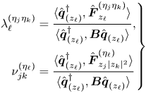 \begin{equation} \left. \begin{aligned} \lambda_{\ell}^{(\eta_j \eta_k)} & = \displaystyle \frac{ \langle {\hat{\boldsymbol{q}}_{(z_{\ell})}^{{{{\dagger}}}}} , {\hat{\boldsymbol{F}}^{(\eta_j \eta_k)}_{z_{\ell}}} \rangle }{ \langle {\hat{\boldsymbol{q}}_{(z_{\ell})}^{{{{\dagger}}}}} , {\boldsymbol{B} \hat{\boldsymbol{q}}_{(z_{\ell})}} \rangle },\\ \nu_{jk}^{(\eta_{\ell})} & = \displaystyle \frac{ \langle {\hat{\boldsymbol{q}}_{(z_{\ell})}^{{{{\dagger}}}}} , {\hat{\boldsymbol{F}}^{(\eta_{\ell})}_{z_j |z_k|^{2}}} \rangle }{ \langle {\hat{\boldsymbol{q}}_{(z_{\ell})}^{{{{\dagger}}}}} , {\boldsymbol{B} \hat{\boldsymbol{q}}_{(z_{\ell})}} \rangle } \end{aligned} \right\} \end{equation}
for  $j,k,\ell = 1,2$.
Appendix B. Non-normality (lift-up and convective mechanisms)
In this section we explore the effect of the non-normal mechanisms on the instability. Two non-normal mechanisms were identified in the flow configuration of the static sphere ( $\varOmega = 0$), cf. Meliga et al. (Reference Meliga, Chomaz and Sipp2009b), the lift-up and convective non-normality mechanisms. The lift-up mechanism is associated with the transport of the steady-state solution by the perturbation, that is, to the component $\hat {\boldsymbol {u}} \boldsymbol {\cdot } \boldsymbol {\nabla } {\boldsymbol {U}_b}$ of (3.2), cf. Marquet et al. (Reference Marquet, Lombardi, Chomaz, Sipp and Jacquin2009). On the other hand, the convective non-normality is due to the advection of disturbances by the steady state, that is, the term ${\boldsymbol {U}_b}\boldsymbol {\cdot } \boldsymbol {\nabla }_m {\hat {\boldsymbol {u}}}$ of (3.2) and $-{\boldsymbol {U}_b}\boldsymbol {\cdot } \boldsymbol {\nabla }_m {\hat {\boldsymbol {u}}^{{{\dagger}} }}$ for the adjoint operator. In physical terms, it corresponds to the convection of disturbances in opposite directions. In terms of direct $\hat {\boldsymbol {q}}$ and adjoint $\hat {\boldsymbol {q}}^{{{\dagger}} }$ global modes, the lift-up non-normality is characterized by the near orthogonality of the direct and adjoint components of velocity because they tend to concentrate in different components of velocity, even if both direct and adjoint modes are active in the same region of space. Instead, the convective non-normality is associated with direct and adjoint modes that tend to be orthogonal because they are localized in different regions of the space. The non-normality may be measured by the angle $\theta _{N}$ (Meliga et al. Reference Meliga, Chomaz and Sipp2009b) defined as
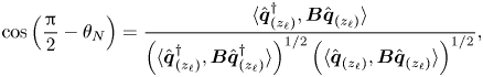 \begin{equation} \cos\left(\frac{\rm \pi}{2} - \theta_{N}\right) = \frac{\langle {\hat{\boldsymbol{q}}_{(z_{\ell})}^{{{{\dagger}}}}} , {\boldsymbol{B} \hat{\boldsymbol{q}}_{(z_{\ell})} } \rangle}{ \left(\langle {\hat{\boldsymbol{q}}_{(z_{\ell})}^{{{{\dagger}}}}} , {\boldsymbol{B} \hat{\boldsymbol{q}}_{(z_{\ell})}^{{{{\dagger}}}} } \rangle\right)^{1/2} \left(\langle {\hat{\boldsymbol{q}}_{(z_{\ell})}} , {\boldsymbol{B} \hat{\boldsymbol{q}}_{(z_{\ell})} } \rangle\right)^{1/2} }, \end{equation}
where the direct and adjoint modes are normalised such that  $\langle {\hat {\boldsymbol {q}}_{(z_{\ell })}^{{{\dagger}} }} , {\boldsymbol {B} \hat {\boldsymbol {q}}_{(z_{\ell })} } \rangle = 1$ and $\langle {\hat {\boldsymbol {q}}_{(z_{\ell })}} , {\boldsymbol {B} \hat {\boldsymbol {q}}_{(z_{\ell })} } \rangle = 1$. It thus measures the departure of $\theta _N$ from ${\rm \pi} /2$ of the angle between direct and adjoint global modes, that is, the smaller the departure the larger the non-normality. However, such a quantity does not suffice to estimate the global effect of each non-normal mechanism, lift-up and convective non-normality. To overcome such an issue, Meliga et al. (Reference Meliga, Chomaz and Sipp2009b) proposed to introduce the estimator $\gamma$ defined as
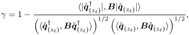 \begin{equation} \gamma = 1 - \frac{\langle { |\hat{\boldsymbol{q}}_{(z_{\ell})}^{{{{\dagger}}}}| } , {\boldsymbol{B} |\hat{\boldsymbol{q}}_{(z_{\ell})}| } \rangle}{ \left(\langle {\hat{\boldsymbol{q}}_{(z_{\ell})}^{{{{\dagger}}}}} , {\boldsymbol{B} \hat{\boldsymbol{q}}_{(z_{\ell})}^{{{{\dagger}}}} } \rangle\right)^{1/2} \left(\langle {\hat{\boldsymbol{q}}_{(z_{\ell})}} , {\boldsymbol{B} \hat{\boldsymbol{q}}_{(z_{\ell})} } \rangle\right)^{1/2} }, \end{equation}
where  $|\hat {\boldsymbol {q}}_{(z_{\ell })}|^{2} = |\hat {\boldsymbol {u}}_{(z_{\ell })}|^{2} + |\hat {p}_{(z_{\ell })}|^{2} = |\hat {{u}}_{(z_{\ell })}|^{2} + |\hat {v}_{(z_{\ell })}|^{2} + |\hat {w}_{(z_{\ell })}|^{2} + |\hat {p}_{(z_{\ell })}|^{2}$ stands for the Euclidean pointwise norm. Such an estimator is used to determine whether the non-normality is due to the lift-up effect or the convective non-normality and it is bounded $0 \leq \gamma \leq 1$. In the case of dominance of the lift-up effect $\gamma$ is close to $0$, i.e. a similar spatial distribution of direct and adjoint modes. On the other hand, a value of $\gamma$ close to unity implies separation in the support of the adjoint and direct global modes.
Appendix C. Unfolding of the triple-Hopf bifurcation
C.1. Classification of solutions
The trivial axisymmetric steady-state solution transits into a rotating wave
 \begin{equation} RW_i = \{ z_j = 0 | \quad \forall j \neq i, \quad i,j=1,2,3 \} \end{equation}
via Hopf-bifurcation. Each of the three types of rotating waves are potential candidates for a primary bifurcation, and they appear in distinct regions of the parameter space  $(\mbox { {Re}},{{\varOmega }})$.
In addition, in the vicinity of the organizing centre of the type (Hopf-Hopf) one can predict the type of secondary bifurcation from each of the rotating waves. Secondary bifurcations of rotating axisymmetric bodies are of mixed-mode type  $MM_{ij}$, $i,j=1,2,3$,
 \begin{equation} MM_{ij} = \{ z_{\ell} = 0 | \quad \forall \ell \neq i, \ell \neq j, \quad i,j,\ell=1,2,3 \}. \end{equation}
Mixed-mode solutions are quasiperiodic solutions with possibly different azimuthal patterns. The transition to a mixed-mode solution  $MM_{12}$ is possible either from $RW_{1}$ or $RW_{2}$ but not from $RW_{3}$. Finally, near a triple-Hopf bifurcation point there may exist a mixed mode composed of three (incommensurate) frequencies, here denoted $IMM_{123}$. This branch can bifurcate from any of the two-frequency component mixed modes $MM_{ij}$, for distinct $i,j=1,2,3$.
C.2. Unfolding amplitude equations – types of solutions
C.2.1. Rotating waves – RW
Rotating waves  $RW_i$ are fixed points of (4.9), where two modes are null, i.e. they satisfy
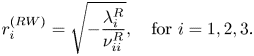 \begin{equation} r_i^{(RW)} = \sqrt{-\frac{\lambda^{R}_i}{\nu_{ii}^{R}}}, \quad \text{for } i = 1,2,3. \end{equation}
Rotating wave solutions are stable if
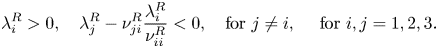 \begin{equation} \lambda_i^{R} > 0, \quad \lambda_j^{R} - \nu_{ji}^{R} \frac{\lambda_i^{R}}{\nu_{ii}^{R}} < 0,\quad \text{for } j \neq i, \quad \text{ for } i,j = 1,2,3. \end{equation}
C.2.2. Mixed modes –  $MM_{ij}$

Mixed-mode solutions  $MM_{12}$ (respectively $MM_{13}$ or $MM_{23}$) are two-component solutions of (4.9) where $r_3 = 0$ (respectively $r_2=0$ or $r_1=0$) and the other two components are non-null. Amplitudes $r_{i}$, $r_{j}$ depend on parameters as follows:
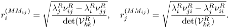 \begin{equation} r^{(MM_{ij})}_i = \sqrt{\frac{\lambda_{j}^{R} \nu^{R}_{ij} - \lambda_{i}^{R} \nu^{R}_{jj} }{ \det(\mathcal{V}^{R}_{kk})}}, \quad r^{(MM_{ij})}_j = \sqrt{\frac{\lambda_{i}^{R} \nu^{R}_{ji} - \lambda_{j}^{R} \nu^{R}_{ii} }{ \det(\mathcal{V}^{R}_{kk}) }}. \end{equation}
Here  $i,j,k=1,2,3$ with $i \neq j$, $k \neq i$ and $k \neq j$.
The Jacobian matrix  $D \boldsymbol {f}^{R}$ can be written in block-diagonal form, which simplifies the stability computations. It is composed of a $2\times 2$ and a $1\times 1$ block. The eigenvalue associated with the $1 \times 1$ block is stable if
 \begin{equation} \sigma_{k} \equiv \frac{1}{\det(\mathcal{V}^{R}_{kk})} \left[\lambda_k^{R} \det(\mathcal{V}^{R}_{kk}) + \lambda_i^{R} \det(\mathcal{V}^{R}_{ik})+ \lambda_j^{R} \det(\mathcal{V}^{R}_{jk}) \right] < 0. \end{equation}
 The  $2\times 2$ block is
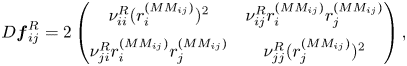 \begin{equation} D\boldsymbol{f}_{ij}^{R} = 2\begin{pmatrix} \nu^{R}_{ii} (r^{(MM_{ij})}_i)^{2} & \nu_{ij}^{R} r^{(MM_{ij})}_i r_{j}^{(MM_{ij})} \\ \nu_{ji}^{R} r^{(MM_{ij})}_i r_{j}^{(MM_{ij})} & \nu^{R}_{jj} (r^{(MM_{ij})}_j)^{2} \end{pmatrix}, \end{equation}
with  $r^{(MM_{ij})}_i r_{j}^{(MM_{ij})} = \sqrt { \lambda _{i}^{R} \lambda _{j}^{R} [ \nu _{ij}^{R}\nu _{ji}^{R} + \nu _{jj}^{R}\nu _{ii}^{R} ] - [(\lambda _i^{R})^{2} \nu _{jj}^{R}\nu _{ji}^{R} + (\lambda _{j}^{R})^{2} \nu _{ii}^{R}\nu _{ij}^{R} ]}/\det (\mathcal {V}^{R}_{kk})$.
The eigenvalues that govern the stability of the mixed-mode solutions of kind  $MM_{ij}$ are the roots of the characteristic polynomial
 \begin{equation} \sigma^{2} - \operatorname{tr}{\left({D\boldsymbol{f}^{R}_{ij}}\right)} \sigma + \det\left(D\boldsymbol{f}_{ij}^{R}\right) = 0, \end{equation}
where
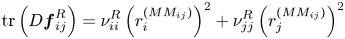 \begin{equation} \operatorname{tr}{\left({D\boldsymbol{f}^{R}_{ij}}\right)} = \nu^{R}_{ii} \left(r^{\left(MM_{ij}\right)}_i\right)^{2} + \nu^{R}_{jj} \left(r^{\left(MM_{ij}\right)}_j\right)^{2} \end{equation}
and
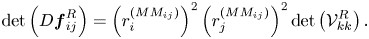 \begin{equation} \det\left(D\boldsymbol{f}_{ij}^{R}\right) = \left(r^{\left(MM_{ij}\right)}_i\right)^{2}\left(r^{\left(MM_{ij}\right)}_j\right)^{2} \det\left(\mathcal{V}^{R}_{kk}\right). \end{equation}
Therefore, one can express the pair of eigenvalues as
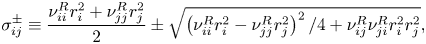 \begin{equation} \sigma^{{\pm}}_{ij} \equiv \frac{ \nu^{R}_{ii} r_i^{2} + \nu^{R}_{jj} r_j^{2} }{2} \pm \sqrt{ \left( \nu^{R}_{ii} r_i^{2} - \nu^{R}_{jj} r_j^{2} \right)^{2}/4 + \nu_{ij}^{R} \nu_{ji}^{R} r_i^{2} r_j^{2} }, \end{equation}
where, for ease of notation, the uperscript  $MM_{ij}$ has been removed. A necessary condition for the Hopf bifurcation of the mixed-mode solutions to occur is that $\nu ^{R}_{ii} \nu ^{R}_{jj} < 0$ and $\nu _{ij}^{R} \nu _{ji}^{R} < 0$. In other words, a Hopf bifurcation from the mixed mode may occur if one of the rotating waves comprised in the mixed mode arises from a supercritical bifurcation whereas the other arises as a result of a subcritical bifurcation from the axisymmetric steady state. This case is discussed in detail in Kuznetsov (Reference Kuznetsov2013, § 8.6) and is denoted as the difficult case. The case where $\nu ^{R}_{ii} \nu ^{R}_{jj} > 0$ is denoted as the simple case, in such a case the mixed-mode solution is a sink or a source located in the separatrix of the basin of attraction of rotating waves.
C.3. Interacting mixed mode – $IMM_{123}$

The  $IMM_{123}$ mode is a $3$-tori solution (phases $\phi _i$ are non-resonant) with their amplitudes determined as the solution of the following linear system:
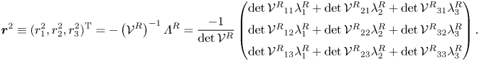 \begin{align} \boldsymbol{r}^{2} \equiv (r_1^{2},r_2^{2},r_3^{2})^{\rm T} ={-} \left( \mathcal{V}^{R} \right)^{{-}1} \varLambda^{R} = \frac{-1}{\det{\mathcal{V}^{R}}} \begin{pmatrix} \det{\mathcal{V}^{R}}_{11} \lambda_1^{R} + \det{\mathcal{V}^{R}}_{21} \lambda_{2}^{R} + \det{\mathcal{V}^{R}}_{31} \lambda_{3}^{R} \\ \det{\mathcal{V}^{R}}_{12} \lambda_{1}^{R} + \det{\mathcal{V}^{R}}_{22} \lambda_{2}^{R} + \det{\mathcal{V}^{R}}_{32} \lambda_{3}^{R} \\ \det{\mathcal{V}^{R}}_{13} \lambda_{1}^{R} +\det{\mathcal{V}^{R}}_{23} \lambda_{2}^{R} + \det{\mathcal{V}^{R}}_{33} \lambda_{3}^{R} \end{pmatrix}. \end{align}
The stability of the interacting mixed-mode solution is determined by the eigenvalues of the Jacobian  $D \boldsymbol {f}^{R}$,
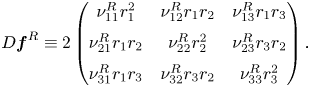 \begin{equation} D \boldsymbol{f}^{R} \equiv 2 \begin{pmatrix} \nu_{11}^{R} r_1^{2} & \nu_{12}^{R} r_1 r_{2} & \nu_{13}^{R} r_1 r_{3} \\ \nu_{21}^{R} r_1 r_{2} & \nu_{22}^{R} r_2^{2} & \nu_{23}^{R} r_3 r_{2}\\ \nu_{31}^{R} r_1 r_{3} & \nu_{32}^{R} r_3 r_{2} & \nu_{33}^{R} r_3^{2} \end{pmatrix}. \end{equation}
The eigenvalues of  $D \boldsymbol {f}^{R}$ are roots of its characteristic polynomial denoted as $p(D \boldsymbol {f}^{R})$,
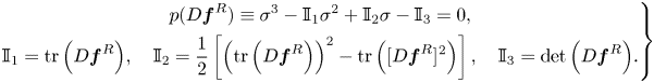 \begin{equation} \left. \begin{gathered} p(D \boldsymbol{f}^{R}) \equiv \sigma^{3} - \mathbb{I}_1 \sigma^{2} + \mathbb{I}_2 \sigma - \mathbb{I}_3 = 0,\\ \mathbb{I}_1 = \operatorname{tr}{ \left( D \boldsymbol{f}^{R} \right) }, \quad \mathbb{I}_2 = \frac{1}{2} \left[ \left( \operatorname{tr}{ \left(D \boldsymbol{f}^{R} \right) } \right)^{2} - \operatorname{tr}{ \left( [D \boldsymbol{f}^{R}]^{2} \right) } \right], \quad \mathbb{I}_3 = \det{\left(D \boldsymbol{f}^{R} \right)}. \end{gathered} \right\} \end{equation}
The trace of the Jacobian can be expressed as a function of the square of the amplitudes  $r_1^{2}, r_2^{2}$ and $r_3^{2}$ and the real part of the matrix of coefficients $\mathcal {V}$,
 \begin{equation} \operatorname{tr}{ \left( D \boldsymbol{f}^{R} \right) } \equiv 2 \left( \nu_{11}^{R} r_1^{2} + \nu_{22}^{R} r_2^{2} + \nu_{33}^{R} r_3^{2} \right), \end{equation}
similarly the second invariant of the Jacobian
 \begin{align} \frac{1}{2} \left[ \left( \operatorname{tr}{ \left(D \boldsymbol{f}^{R} \right) } \right)^{2} - \operatorname{tr}{ \left( [D \boldsymbol{f}^{R}]^{2} \right) } \right] \equiv 4\left(r_1^{2} r_2^{2} \det{\mathcal{V}^{R}_{33}} + r_1^{2} r_3^{2} \det{\mathcal{V}^{R}_{22}} +r_2^{2} r_3^{2} \det{\mathcal{V}^{R}_{11}}\right), \end{align}
and the determinant
 \begin{equation} \det{\left(D \boldsymbol{f}^{R} \right) = 8 r_1^{2} r_2^{2} r_3^{2} \det{\mathcal{V}^{R}}}. \end{equation}
 The characteristic polynomial (C14) is a cubic polynomial with real coefficients. Thus, the eigenvalues  $\sigma$ of the Jacobian $D \boldsymbol {f}^{R}$ are either all real or one of them is real and the other two are complex conjugate. The nature of the eigenvalues depends on the discriminant of the cubic equation. A stationary bifurcation occurs when $\det (D \boldsymbol {f}^{R} ) = 0$, which under the generic condition $\det {\mathcal {V}^{R}} \neq 0$ only occurs at the origin of the $IMM_{123}$.
A Hopf bifurcation arises when the following conditions are satisfied:
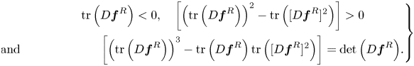 \begin{equation} \left. \begin{aligned} & \operatorname{tr}{\left(D \boldsymbol{f}^{R} \right) } < 0, \quad \left[ \left( \operatorname{tr}{ \left(D \boldsymbol{f}^{R} \right) } \right)^{2} - \operatorname{tr}{ \left( [D \boldsymbol{f}^{R}]^{2} \right) } \right] > 0\\ & \hspace{-64pt}\text{and}\hspace{64pt} \left[ \left( \operatorname{tr}{ \left(D \boldsymbol{f}^{R} \right) } \right)^{3} - \operatorname{tr}{\left(D \boldsymbol{f}^{R} \right) } \operatorname{tr}{ \left( [D \boldsymbol{f}^{R}]^{2} \right) } \right] = \det{ \left(D \boldsymbol{f}^{R} \right) }. \end{aligned} \right\} \end{equation}
 The condition 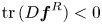 $\operatorname {tr}{(D \boldsymbol {f}^{R} ) } < 0$ ensures that Hopf bifurcation is the primary bifurcation of the $IMM_{123}$ solution, i.e. the real eigenvalue is negative. Such a condition holds true in the supercritical case, when $\nu _{ii} < 0$, for $i=1,2,3$. Additionally, there is a change in the nature of the solution $IMM_{123}$ whenever the discriminant changes sign, it changes from sink to stable foci, from source to unstable foci, from saddle to saddle foci or vice versa. Even though these local changes in the nature of the fixed-point solution $IMM_{123}$ cannot be considered as a local bifurcation, they could be linked to global changes in dynamics, e.g. the appearance of a heteroclinic cycle as in the difficult case of a Hopf-Hopf bifurcation (Kuznetsov Reference Kuznetsov2013, Ch. 8.7.). Finally, a necessary and sufficient condition for the stability of the asymptotic stability of the $IMM_{123}$ solution can be expressed in terms of the invariants of the Jacobian matrix
 \begin{equation} \mathbb{I}_1 < 0, \quad \mathbb{I}_2 > 0, \quad \mathbb{I}_3 < 0, \quad \mathbb{I}_1 \mathbb{I}_2 > \mathbb{I}_3. \end{equation}
Inspection of (C19) shows that the condition for the Hopf bifurcation indeed corresponds to the limit case of the condition  $\mathbb {I}_1 \mathbb {I}_2 \geq \mathbb {I}_3$.
Appendix D. Mesh convergence
Mesh independent solutions have been verified systematically. First, we have considered a given mesh refinement, and we have varied the physical size of the domain. We have observed that, for a domain length of  $50$ diameters downstream of the sphere centre, $20$ diameters upstream of the cylinder centre and $20$ in the cross-stream direction, the effects of the boundary condition do not have an effect on the solution. Secondly, we have looked at the effect of mesh refinement on the properties of the solution. For that purpose, we performed a parametric study of eigenvalues, normal form coefficients of the codimension-two point $B$ (table 8). Every mesh is initially computed by Delauny triangulation, and subsequently adapted to either base flow, eigenmode or both, following the methodology described in Fabre et al. (Reference Fabre, Citro, Ferreira Sabino, Bonnefis, Sierra, Giannetti and Pigou2018); and their properties are summarised in table 7.
Table 7. Properties of the meshes used in the study of mesh convergence.
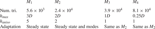
Table 8. Cubic coefficients of the normal form (4.9) evaluated at the codimension-two point  $A$.
$A$.
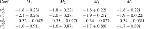
Appendix E. Higher-order dynamic mode decomposition
This analysis allows us to gain valuable insight on the dominant modes and associated spatio-temporal flow structures which govern the wake for the different regimes encountered in our transition scenario (figure 9). As detailed by Le Clainche & Vega (Reference Le Clainche and Vega2017a), Vega & Le Clainche (Reference Vega and Le Clainche2020), HODMD is an extension of the standard dynamic mode decomposition (DMD) technique (Schmid Reference Schmid2010), which has been proven useful to study flow structures associated with quasiperiodic (featuring a large number of frequencies) or transitional regimes (Le Clainche & Vega Reference Le Clainche and Vega2017b), where the classical DMD approach may fail, being therefore applicable to complex spectral and spatial cases, as the problem investigated herein. The number of modes identified by HODMD is determined by  $M$, whose value is related to the spatial resolution of the input data, and $N$, determined by the temporal resolution.
Thus, the present HODMD tool has been applied to resolve the spatial structure related to dominant frequencies characterizing the different flow regimes identified from the DNS results. Typically, the input data consists of a set of  $N = 2000$ streamwise vorticity, $\varpi _z$, snapshots interpolated in a 80 $\times$80 ( $M=6400$) rectangular grid whose domain is $(x,y) \in [-1,1]$ located at $z = 2.5$. Moreover, it should be noted that the vorticity snapshots are equally spaced in time with a $\Delta t = 0.15$. Such temporal parameters allow us to resolve frequencies between $St_{min}=0.003$ and $St_{max}=3.33$, according to the Nyquist criterion. Given such input data, which satisfies the condition $N< M$, the values of the main HODMD parameters, i.e. order, $d$, and tolerance, $\epsilon$, have been calibrated and fixed at $d=50$ and $\epsilon = 1e-6$ to capture a great number of modes.
Appendix F. The 0-1 test
The quantitative 0-1 method (Gottwald & Melbourne Reference Gottwald and Melbourne2004) is used to evaluate the dynamic complexity and likely chaotic nature of the flow regimes. The method is directly applied to time series of any scalar, as the pointwise fluctuating radial velocity  $U'$. In particular, given a set of data from velocity of $N$ samples, $U'(j)$ with $j=1,\ldots,N$, a translation variable is defined as $p(m) = \varSigma _{j=1}^{m_s} U'(j) \cos (j s)$, for $m = 1,\ldots, m_s$ and $s\in (0, {\rm \pi}/5)$. The mean square displacement is defined as $M_c(m)= \lim _{N\rightarrow \infty } ({1}/{N})\varSigma _{j=1}^{N}[p_c(j+m)-p(j)]^{2}$, which requires that $m_s\leq N$ (as in Gottwald & Melbourne (Reference Gottwald and Melbourne2004), we use $m_s=N/10$). Thus, the variable $M_c(m)$ is bounded when $p(j)$ is also bounded which is the case for regular dynamics. However, if the translation variable $p(m)$ is chaotic, $M_c(m)$ grows linearly with $m$, so that an asymptotic growth $K$ can be defined as
 \begin{equation} K = \lim_{m\rightarrow \infty} \frac{\log(M_c(m))}{\log(m)}, \end{equation}
which will take the value of 1 for chaotic dynamics and 0 for regular dynamics. Further information and validation of the use of this estimate to evaluate the dynamic nature of complex flow regimes can be found in Lorite-Díez & Jiménez-González (Reference Lorite-Díez and Jiménez-González2020).


 Open access