


1 Introduction
The earliest formulation of mirror symmetry relates pairs of d-dimensional Calabi–Yau manifolds  $X, X^{\vee }$ with mirror Hodge diamonds:
 $$\begin{align*}h^{p,q}(X)=h^{d-p,q}(X^{\vee}).\end{align*}$$
In the early 1990s, physicists Greene, Morrison and Plesser found many such mirror pairs [Reference Greene, Morrison and Plesser23], starting with a Calabi–Yau (and Fermat) hypersurface in projective space and constructing a mirror, which is a resolution of the quotient of the same hypersurface by a finite group. In 1992, this construction was generalized by Berglund–Hübsch [Reference Berglund and Hübsch5], starting with a Calabi–Yau orbifold given as a quotient of a more general hypersurface in weighted projective spaces by a finite group. The hypersurface is a Calabi–Yau orbifold defined as the zero locus of a quasi-homogenous polynomial  $W=\sum _{i=0}^n \prod _{j=0}^n x_{j}^{m_{ij}}$ such that W is nondegenerate and ‘invertible’ (i.e., with as many variables as monomials). After quotienting out by a finite group H of diagonal symmetries within $\operatorname {SL}(n+1;{\mathbb C})$ one obtains the orbifold $\Sigma _{W,H}$. The mirror $\Sigma _{W^{\vee },H^{\vee }}$ is another such quotient of a hypersurface modulo a finite group. The hypersurface is given by the polynomial $W^{\vee }$, defined by transposing the matrix of the exponents $E=[m_{ij}]$ of W. The group $H^{\vee }$ is a subgroup of $\operatorname {SL}(n+1;{\mathbb C})$ Cartier dual to H and preserving $W^{\vee }$; see equation (19). Then, the mirror duality can be stated in terms of orbifold Chen–Ruan cohomology as
 $$ \begin{align} H_{\operatorname{CR}}^{p,q}(\Sigma_{W,H};{\mathbb C})=H_{\operatorname{CR}}^{d-p,q}(\Sigma_{W^{\vee},H^{\vee}};{\mathbb C}), \end{align} $$
which implies the same relation in ordinary cohomology whenever there exists crepant resolutions.
The striking mirror relation above appears more natural when we look at it through the lens of singularity theory or, in physics terminology, the Landau–Ginzburg (LG) model. This happens because mirror symmetry holds for LG models without any Calabi–Yau condition. In this paper, we present this change of perspective through the LG model via the crepant resolution of a singularity; see Section 5. This not only allows us to simplify previous proofs of LG/CY correspondence by the first author with Ruan [Reference Chiodo and Ruan9]; it also yields a new statement of mirror symmetry relating the fixed loci of powers of an isomorphism s of  $\Sigma $, the Hodge decomposition and the weights the representation $s^*$ in cohomology.
Let  $W=x_0^k+f(x_1,\dots ,x_n)$ be a nondegenerate, quasi-homogenous, invertible polynomial. Let us consider again the automorphisms groups $H\subseteq \operatorname {Aut} W$ and its dual $H^{\vee }\in \operatorname {Aut} W$ within $\operatorname {SL}(n+1;{\mathbb C})$. The Calabi–Yau orbifolds $\Sigma _{W,H}$, $\Sigma _{W^{\vee },H^{\vee }}$ are equipped with the action by the group ${\pmb \mu }_k$ of kth roots of unity spanned by $s\colon x_0 \mapsto e^{2\pi i/k} x_0$. For i in the group of characters ${\mathbb Z}/k=\operatorname {Hom}({\pmb \mu }_k;{\mathbb G}_m)$ we consider the weight-i term of cohomology
 $$ \begin{align*} H^*(\text{---},{\mathbb C})_{i}=\{x\mid s^*x=i(s)x\}. \end{align*} $$
The first statement is that the s-invariant cohomology mirrors the ‘moving’ cohomology: the sum of all cycles of nonvanishing weight.
Theorem A (see Theorem 44, part 1)
Consider  $s\colon \Sigma _{W,H}\to \Sigma _{W,H}$ and its mirror partner $s\colon \Sigma _{W^{\vee },H^{\vee }}\to \Sigma _{W^{\vee },H^{\vee }}$. We have
 $$\begin{align*}H^{p,q}_{orb}(\Sigma_{W,H};{\mathbb C})_{0}\cong \bigoplus_{i=1}^{k-1} H^{d-p,q}_{orb}(\Sigma_{W^{\vee},H^{\vee}};{\mathbb C})_{i}, \end{align*}$$
 where  $d=n-1$ is the dimension of $\Sigma _{W,H}$.
The locus of geometric points of  $\Sigma _{W,H}$ which are fixed by s also exhibits a mirror phenomenon. Since $\Sigma _{W,H}$ is a stack, let us provide a definition for this s-fixed locus. For s a finite order automorphism acting on a smooth Deligne–Mumford orbifold ${{\mathfrak X}}$, we consider the graph of $\Gamma _s\colon {{\mathfrak X}}\to {{\mathfrak X}}\times {{\mathfrak X}}$ and its intersection with the graph of the identity (the diagonal morphism)
 $$\begin{align*}{{\mathfrak X}}{\underset{s, \ {{\mathfrak X}}\times {{\mathfrak X}}, \ \operatorname{id}}{\times}}{{\mathfrak X}}, \end{align*}$$
(we write s and  $\operatorname {id}$ instead of the respective graphs). We recall that orbifold cohomology is the (age-shifted) cohomology of this product for $s=\operatorname {id}$. Then, we define the s-orbifold cohomology as the age-shifted cohomology of the above fibred product in general (see Definition 7). This is a bigraded vector space, and, if the coarse space X of ${\mathfrak X}$ admits a crepant resolution $\widetilde X$ where s lifts, there is a bidegree-preserving isomorphism $H_s^*({\mathfrak X};{\mathbb C})\cong H_s^*(\widetilde X;{\mathbb C}),$ where the right-hand side is the age-shifted cohomology of the s-fixed locus in $\widetilde X$; see Proposition 9.
We can now state two mirror dualities for  $s^j$-fixed loci in this sense. Under the same conditions on W and H as above, set $\Sigma =\Sigma _{W,H}$ and $\Sigma ^{\vee }=\Sigma _{W^{\vee },H^{\vee }}$. If the order k of s is not prime, then s acts nontrivially on the fixed locus of powers of s. The s-moving cohomology of the fixed locus of powers of s mirrors the same on $\Sigma ^{\vee }$, interweaving the weight and the exponent of the power of s.
Theorem B (see Thm 44, part 3)
Let  $0<b,t<k$. Then, we have
 $$\begin{align*}\textstyle{H^{p,q}_{s^b}(\Sigma)\left(\frac{b}k\right)_{t}\cong H^{d-p,q}_{s^{-t}}(\Sigma^{\vee})\left(\frac{k-t}k\right)_{-b}}, \end{align*}$$
where  $d=n-2$, the largest dimension of the components of the s-fixed locus.
Finally, also the fixed cohomology of each power  $s^j$ exhibits a mirror phenomenon but only after adding certain moving cycles in $\Sigma $. Namely, the cycles we add are all those whose weight differs from $0$ (i.e., moving cycles) and from j (the exponent of s). We denote this group by $\overline {H}^{p,q}_{\operatorname {id},j}(\Sigma )$; see equation (34).
Theorem C (see Theorem 44, part 2)
For  $0<j<k$, we have
 $$ \begin{align*} \left[H^{p,q}_{s^j}(\Sigma)\left(\tfrac{j}{k}\right)\right]^s \oplus \overline{H}^{p,q}_{\operatorname{id},j}(\Sigma)\cong \left[H^{d-p,q}_{s^j}(\Sigma^{\vee})\left(\tfrac{j}{k}\right)\right]^s \oplus \overline{H}_{\operatorname{id},j}^{d-p,q}(\Sigma^{\vee}). \end{align*} $$
The correcting terms  $\overline {H}^{*}$ disappear when $k=2$ (for $k=2$, we have $s^j=s$ and there is no positive weight except $1$). This shows how the statement above specialises to the construction of Borcea–Voisin mirror pairs, which can be stated as a mirror duality between the s-fixed loci (see [Reference Chiodo, Kalashnikov and Veniani12]).
In dimension 2, and after resolving, these results are about mirror symmetry for K3 surfaces with nonsymplectic automorphisms. Suppose X and  $X^{\vee }$ are crepant resolutions of $\Sigma _{W,H}$ and $\Sigma _{W^{\vee },H^{\vee }}$, where W is a polynomial in $4$ variables. The above mirror theorems imply that the topological invariants of the fixed locus of the K3 surface X controls that of $X^{\vee }$; we refer to Corollary 51 for simple formulae on the number of fixed points and the genera of the fixed curves. The automorphism s also gives the K3 surface a lattice polarization: $H^2(X,{\mathbb Z})^s$. There is another version of mirror symmetry for lattice polarized K3 surfaces, arising from the work of Nikulin [Reference Nikulin28], Dolgachev [Reference Dolgachev18], Voisin [Reference Voisin35] and Borcea [Reference Borcea6]. When the order of s is odd and prime, this lattice is characterised by the invariants $(r,a)$: the rank and the discriminant. Families of lattice polarized K3 surfaces come in mirror pairs, and in the odd prime case this mirror symmetry takes a lattice with invariants $(r,a)$ to $(20-r,a)$. The following corollary is a theorem of Bott, Comparin, Lyons, Priddis and Suggs [Reference Comparin, Lyons, Priddis and Suggs14, Reference Comparin and Priddis15, Reference Bott, Comparin and Priddis8] proven by case-by-case analysis. Here, it is shown directly from the above statements (see Theorem 53).
Corollary ([Reference Comparin, Lyons, Priddis and Suggs14, Reference Comparin and Priddis15, Reference Bott, Comparin and Priddis8])
Let p be prime and different from  $2$. Let $\Sigma _{W,H}$ and $\Sigma _{W^{\vee },H^{\vee }}$ be mirror K3 orbifolds with order-p automorphisms $s, s^{\vee }$, and let $\Sigma $ and $\Sigma ^{\vee }$ be crepant resolutions with automorphisms also denoted $s, s^{\vee }$. Then $\Sigma $ and $\Sigma ^{\vee }$ are mirror as lattice polarized K3 surfaces.
1.1 Relation to previous work
This paper generalises the results of [Reference Chiodo, Kalashnikov and Veniani12]. There, only involutions were considered; here, the mirror theorems apply to automorphism of any order. There, Theorems A and C are simpler (invariant classes mirror anti-invariant classes in Theorem A and no extra terms appear in Theorem C). Theorem B does not apply in the involution case. In the above corollary, we do not consider the order-2 case treated in [Reference Chiodo, Kalashnikov and Veniani12]; in the present paper, this allows us to deduce the lattice mirror symmetry statement of [Reference Comparin, Lyons, Priddis and Suggs14] in full.
Section 5 restates and recasts the proof of mirror symmetry through LG models and the correspondence between cohomology and LG models in terms of resolutions of singularities (see Theorem 31). This may be regarded as the outcome of the work of many authors, we refer to [Reference Krawitz26], [Reference Borisov7], [Reference Kaufmann25] [Reference Chiodo and Ruan9], [Reference Ebeling and Takahashi19], [Reference Ebeling and Gusein-Zade20] and [Reference Ebeling and Gusein-Zade21] and [Reference Chiodo and Nagel13] validating over the years the approach of the physicists Intriligator–Vafa [Reference Intriligator and Vafa24] and Witten [Reference Witten36]. It is also worth mentioning that the main object of our study, a polynomial  $W=x_0^k + f(x_1,\ldots ,x_n)$ with the cyclic symmetry group of kth roots of unity acting on $x_0$, was used in Varchenko’s proof of semicontinuity of Steenbrink’s spectra of singularities [Reference Varchenko32] and [Reference Steenbrink31]. We hope that this may lead to further explanations of mirror symmetry in the framework of singularity theory. In particular, our setup only concerns hypersurfaces in weighted projective space; it would be interesting to see if it extends to other contexts where mirror constructions are known.
Finally, it is worth mentioning that the work of Bott, Comparin, Lyons, Priddis and Suggs [Reference Comparin, Lyons, Priddis and Suggs14]; earlier work of Artebani, Boissière and Sarti [Reference Artebani, Boissière and Sarti2] and more generally Nikulin’s classification [Reference Nikulin28] yield several tables summarising explicit treatments of K3 surfaces via resolution of singularities. Much of these data are now embodied into the s-weighted Hodge numbers of Theorems A, B and C. We provide some examples for this in the tables at the end of §7.
1.2 Structure of the paper
Section 2 states notation and terminology. Section 3 presents the Berglund–Hübsch mirror symmetry construction. Section 4 sets up our generalisation of orbifold cohomology sensing the s-fixed locus: s-orbifold cohomology. Section 5 illustrates and reproves the transition to Landau–Ginzburg models which is crucial in the proof. In particular it provides a straightforward description of the LG/CY correspondence from the crepant resolution conjecture without using the combinatorial model of [Reference Chiodo and Ruan9]. Section 6 is the technical heart of the paper; it proves the main theorem (Theorem 43) on the LG side. Section 7 translates the result from the LG side to the CY side. It contains Theorem 44 proving the statements A, B and C and Theorem 53 specialising to K3 surfaces.
Acknowledgements
We are grateful to Behrang Noohi, whose explanations clarified inertia stacks to us. We are grateful to Baohua Fu, Lie Fu, Dan Israel and Takehiko Yasuda for many helpful conversations. We thank Davide Cesare Veniani, with whom we started studying involutions of Calabi–Yau orbifolds, for continuing to share his insights and expertise. We are extremely grateful to the referee, whose requests made some statements more precise, corrected some mistakes and improved the readability of the paper.
2 Terminology
Deligne–Mumford orbifolds are smooth separated Deligne–Mumford stacks with a dense open subset isomorphic to an algebraic variety.
2.1 Conventions
We work with schemes and stacks over the complex numbers. All schemes are Noetherian and separated. By linear algebraic group we mean a closed subgroup of  $\operatorname {GL}(m\,;{\mathbb C})$ for some m.
2.2 Notation
We list here notation that occurs throughout the entire paper.

Remark 1 (zero loci)
We add the subscript  ${\mathbb P}({\pmb w})$ when we refer to the zero locus in ${\mathbb P}({\pmb w})$ of a polynomial f which is ${\pmb w}$-weighted homogeneous. In this way, we have
 $$\begin{align*}Z_{{\mathbb P}({\pmb w})}(f)=[U/{\mathbb G}_m],\qquad \text{ with } U=Z(f)\subset {\mathbb C}^n\setminus \pmb 0. \end{align*}$$
Remark 2 (zero dimensional  ${\mathbb P}(d)$ for $d\in \mathbb N^*$)


For d a positive integer, we write  ${\mathbb P}(d)$ for the stack $[{\mathbb C}^{\times }/{\mathbb G}_m]$, isomorphic to $B{\pmb \mu }_d$ if $\lambda \in {\mathbb G}_m$ operates on z as $\lambda \cdot z=\lambda ^dz$.
Remark 3 (degree shift)
We often write  $H(a)$ for $H(a,a)$.
Remark 4 (cohomology coefficients)
We only consider cohomology with coefficients in  ${\mathbb C}$; therefore, we sometimes write $H^*(X;{\mathbb C})$ as $H^*(X).$
Remark 5 (graphs and maps)
Given an automorphism  $\alpha $ of ${\mathfrak X}$, we write $\Gamma _{\alpha }$ for the graph ${\mathfrak X}\to {\mathfrak X}\times {\mathfrak X}$. However, to simplify formulæ, we often abuse notation and use $\alpha $ for the graph $\Gamma _{\alpha }$ as well as the automorphism. In this way, in subscripts, the diagonal $\Delta \colon {\mathfrak X}\to {\mathfrak X}\times {\mathfrak X}$ will be often written as $\operatorname {id}_{{\mathfrak X}}$ or simply $\operatorname {id}$.
3 Setup
We recall the general setup of nondegenerate polynomials P where the theory of Jacobi rings applies. Then we introduce polynomials of the special form
 $$ \begin{align*} W(x_0,x_1,\dots,x_n)=x_0^k+f(x_1,\dots, x_n) \end{align*} $$
for  $n>0$.
3.1 Nondegenerate polynomials
We consider quasi-homogeneous polynomials P of positive degree d and of positive weights  $w_0,\dots ,w_n$ satisfying
 $$ \begin{align*} P(\lambda^{w_0}x_0,\dots,\lambda^{w_n}x_n)=\lambda^dP(x_0,\dots,x_n), \end{align*} $$
for all  $\lambda \in {\mathbb C}$. We assume that the polynomial P is nondegenerate; i.e., the choice of weights and degree is unique and the partial derivatives of W vanish simultaneously only at the origin. We consider the zero locus
 $$ \begin{align*} \Sigma_P=Z_{{\mathbb P}({\pmb w})}(P)\subset {\mathbb P}({\pmb w}) \end{align*} $$
which is, by nondegeneracy, a smooth hypersurface within the weighted projective stack  ${\mathbb P}({\pmb w})= [({\mathbb C}^{n+1}\setminus \pmb 0)/{\mathbb G}_m]$ with ${\mathbb G}_m$ acting with weights $w_0,\dots ,w_n$. The polynomial is of Calabi-Yau type if
 $$ \begin{align} \sum_{i=0}^n{w_i}=d. \end{align} $$
This implies that the canonical bundle of  ${\Sigma _P}$ is trivial; we refer to $\Sigma _P$ as a Calabi–Yau orbifold.
Because P is nondegenerate, the group of its diagonal automorphisms
 $$ \begin{align*} \operatorname{Aut}_P=\{\mathrm {diag}(\alpha_0,\dots,\alpha_n)\mid P(\alpha_0x_0,\dots, \alpha_nx_n)=P(x_0,\dots,x_n)\} \end{align*} $$
is finite. Indeed, the  $h\times ({n+1})$ exponent matrix $E=(m_{i,j})$ defined by the condition $P=\sum _{i=1}^h c_i \prod _{j=0}^n x_j^{m_{i,j}}$ is left invertible as a consequence of the uniqueness of the vector $\left ({w_i}/{d}\right )_{i=0}^n=E^{-1}{\pmb 1}.$
Since we are working over  ${\mathbb C}$, we adopt the notation
 $$ \begin{align*} [a_0,\dots,a_n]=\mathrm {diag}(\exp(2\pi\mathtt{i} a_i))_{i=0}^n \end{align*} $$
for  $a_i\in \mathbb Q\cap [0,1[$. The age of the diagonal matrix above is
 $$ \begin{align} \mathrm{age}[a_0,\dots,a_n]=\sum_{i=0}^na_i. \end{align} $$
The distinguished diagonal symmetry
 $$ \begin{align*} j_P=\left[\frac{w_0}{d},\dots,\frac{w_n}{d}\right], \end{align*} $$
usually denoted by j, spans the intersection  $\operatorname {Aut}_P\cap \,{\mathbb G}_m$, where ${\mathbb G}_m$ is the group of automorphisms of the form $\mathrm {diag}(\lambda ^{w_0},\dots ,\lambda ^{w_n})$. The group element $j_P$ has a natural interpretation as a monodromy operator of the fibration defined by P restricted to the complement in ${\mathbb C}^{n+1}$ of the zero locus $Z(P)$; see, for instance, [Reference Dimca17]. We will denote by $M_P$ the generic Milnor fibre

For any subgroup H of  $\operatorname {Aut}_P$ containing $j_P$, we consider the Deligne–Mumford stacks
 $$ \begin{align*} \Sigma_{P,H}=[\Sigma_P/H_0],\qquad M_{P,H}=[M_P/H], \end{align*} $$
where  $H_0=H/(H\cap {\mathbb G}_m)=H/\langle j\rangle $ and acts faithfully on $\Sigma _P$. The orbifold $\Sigma _{P,H}$ is a smooth codimension- $1$ substack of $[{\mathbb P}({\pmb w})/H_0]$
 $$ \begin{align*} \Sigma_{P,H}\subset [{\mathbb P}({\pmb w})/H_0], \end{align*} $$
and has trivial canonical bundle if P is Calabi–Yau in the sense of equation (2) and H lies in
 $$ \begin{align*} \operatorname{SL}_P:=\operatorname{Aut}_P\cap \operatorname{SL}(n+1;{\mathbb C}). \end{align*} $$
3.2 Polynomials with automorphism
We focus on polynomials of Calabi–Yau type of the form
 $$ \begin{align*} W(x_0,x_1,\dots,x_n)=(x_0)^k+f(x_1,\dots,x_n). \end{align*} $$
We have  $\operatorname {Aut}_W={\pmb \mu }_k\times \operatorname {Aut}_f$, where, using again the choice $\exp (2\pi i/k)$, the first factor is regarded here as ${\mathbb Z}/k$, canonically generated by the order-k automorphism
 $$ \begin{align} s=\left[\frac1k,0,\dots,0\right]. \end{align} $$
The second factor is regarded as the subgroup of  $\operatorname {Aut}_W$ formed by symmetries fixing the first coordinate. We have $j_W=s\cdot j_f$, with $s\in {\mathbb Z}/k$ and $j_f\in \operatorname {Aut}_f$. Notice that the group ${\mathbb Z}/k$ acts on the stack $\Sigma _{W,H}$
 $$ \begin{align*} \mathsf{m}\colon ({\mathbb Z}/k)\times \Sigma_{W,H}\to \Sigma_{W,H}. \end{align*} $$
 Instead of considering all groups  $H\subseteq \operatorname {Aut} W\cap \operatorname {SL}(n+1;{\mathbb C})$ containing $j_W$, we can equivalently consider their intersections with $\operatorname {Aut}_f$. In this way, since the first coordinate of $(j_W)^h$ equals $1$ if and only if $h\in k{\mathbb Z}$, we obtain all the subgroups $K \subset \operatorname {Aut}_f$ satisfying
 $$ \begin{align*} (j_f)^k\in K\subseteq \operatorname{SL}_f. \end{align*} $$
We recover the previous subgroups H of  $\operatorname {Aut} W\cap \operatorname {SL}(n+1;{\mathbb C})$ as the subgroups of $\operatorname {Aut}_W$ spanned by $j_W$ and K.
Our mirror duality requires a slightly more general class of groups. Therefore, we consider the subgroup of  $\operatorname {Aut}_W$
 $$ \begin{align*} K[j_W,s]=\sum_{a,b=0}^{k-1} (j_W)^{a}(s)^{b}K, \end{align*} $$
with its natural  $(\frac 1k{\mathbb Z}/{\mathbb Z})$-gradings
 $$ \begin{align*} d_j=\frac{a}{k},\qquad d_s=\frac{b}{k}. \end{align*} $$
By the condition  $\sum _{i=0}^n w_i=d$, the determinant of an element $g\in K[j_W,s]$ equals $\exp (2\pi \mathtt {i} d_s(g))$. The condition $d_s=0$ singles out the groups which we considered initially: $H\subseteq \operatorname {Aut} W\cap \operatorname {SL}(n+1;{\mathbb C})$ containing $j_W$.
4 Variants of orbifold Chen–Ruan cohomology
We introduce this section by a short description of the variant of cohomology group needed in this paper and by a motivation via its main application.
For any finite order automorphism g of a stack  ${\mathfrak X}$, we define g-orbifold cohomology, a slight generalization of orbifold Chen–Ruan cohomology; see Definition 7. The setup follows the original definition of orbifold Chen–Ruan cohomology: the cohomology of the inertia stack whose grading is shifted by the locally constant rational age function. Here, we start from the g-inertia stack, which is a g-dependent version of the ordinary inertia stack corresponding to $g=\operatorname {id}_{{\mathfrak X}}$. Then, as in the ordinary case, we take its cohomology with complex coefficients after a degree-shift by the same age function. The treatment provided here improves [Reference Chiodo, Kalashnikov and Veniani12], where the g-inertia stack was obtained via a new ad hoc construction. Here, we produce the g-inertia stack as a union of connected components of the inertia stack of $[{\mathfrak X}/G]$, where G is a group acting on ${\mathfrak X}$ and containing g. The definition of the age function is then straightforward via the natural inclusion within the larger inertia stack of $[{\mathfrak X}/G]$ and by restriction of the usual age function.
We recall that the main interest of orbifold Chen–Ruan cohomology is its identification with the ordinary cohomology of certain resolutions of coarse quotients in terms of their orbifold (i.e., stack-theoretic) presentation. Because the g-inertia stack of a space X is simply the g-fixed locus, the present setup allows an analogous statement for g-fixed loci; see Proposition 9. In fact, the orbifold and the crepant resolution can be described as K-equivalent (a relation holding when the canonical sheaves match). Indeed, the canonical bundle of the stack descends from the orbifold to the coarse space and matches the canonical bundle of the resolution via pullback. In this perspective, the identification of cohomology groups follows from a result by Yasuda, [Reference Yasuda37] on invariance under K-equivalence of motivic cohomology. In Proposition 9, we check that his result applies to our slightly more general setup. We point out that, in [Reference Chiodo, Kalashnikov and Veniani12, Prop. 4.7.2], we proved all this explicitly via a direct argument which holds only in dimension two.
We now introduce the G-inertia stack. The construction parallels the presentation of the inertia stack of a quotient stack  $[U/G]$, where U is a scheme and G is a group, which is in turn a quotient stack $[I_G(U)/G]$, where $I_G(U)$ is the G-inertia group scheme (a group scheme referred to as ‘the stabilizer of the groupoid’ in [29, Lem. 70.25.1]) modulo a natural G-action. What follows is the analogue definition when the scheme U is replaced by a Deligne–Mumford stack ${\mathfrak X}$ (see [Reference Chiodo, Kalashnikov and Veniani12, §4.3] for an earlier version of this). This is again a special case of the above-mentioned G-inertia group scheme construction of [29, Lem. 70.25.1]. Here, we illustrate how these notions can be made more explicit in the present setup.
We consider a finite group G acting on a Deligne–Mumford orbifold  ${\mathfrak X}$
 $$ \begin{align*} \mathsf{m}\colon G\times {\mathfrak X} \to {\mathfrak X}. \end{align*} $$
The G-inertia stack  $I_G({\mathfrak X})$ fits in the following fibre diagram

When G is a trivial group,  $I{\mathfrak X}$ is the ordinary inertia of ${\mathfrak X}$.
In this way, we have
 $$ \begin{align*} I_G({\mathfrak X})=(G\times {\mathfrak X})\times_{(\mathsf{m},\mathsf{pr_2}),\, {\mathfrak X}\times {\mathfrak X},\,\Delta}{\mathfrak X}=\bigsqcup_{g\in G} I_g({\mathfrak X}), \end{align*} $$
where  $I_g({\mathfrak X})$ is the g-inertia orbifold
 $$ \begin{align} I_g({\mathfrak X}):={\mathfrak X}{\underset{g, \ {\mathfrak X}\times {\mathfrak X}, \ \operatorname{id}}{\times}}{\mathfrak X}. \end{align} $$
 The G-inertia stack of  ${\mathfrak X}$ can be naturally related to the ordinary inertia stack of $[{\mathfrak X}/G]$. Indeed, we have the fibre diagram

and we may regard  ${\mathsf p}$ as a G-torsor by pullback of ${\mathfrak X}\to [{\mathfrak X}/G]$.
The G-action on  $\bigsqcup _{g\in G} I_g{\mathfrak X}$ is given by conjugation on the indices and by $F_h \colon I_g {\mathfrak X} \to I_{hgh^{-1}} {\mathfrak X}$ on the components, where $F_h$ acts by the effect of h on the first factor of equation (6) and by the identity on the second factor.
Remark 6. In this paper, we only consider quotient stacks of the form  $[U/H]$, where H is an abelian group with finite stabilizers. Then, as in [Reference Chiodo, Kalashnikov and Veniani12, Defn. 4.3.2], unraveling the above definitions yields a presentation of $I_g[U/H]$ (denoted by ‘ $\mathfrak I_{[U/H]}^g$’ there) as the quotient stack $[I_{gH}(U)/H]$, where $I_{gH}(U)$ equals $\{(gh,x)\mid gh\cdot x=x\}$ and the group H operates on the second factor.
4.1 A g-orbifolded cohomology
The g-orbifold cohomology is the cohomology of  $I_g({\mathfrak X})$ defined in equation (6) shifted by the locally constant function ‘age’ given by ${\mathfrak a}_g={\mathfrak a}\circ {\mathsf p}$
 $$ \begin{align} {\mathfrak a}_g\colon I_g({\mathfrak X})\xrightarrow{{\mathsf p}} I[{\mathfrak X}/G]\xrightarrow{{\mathfrak a}} \mathbb Q, \end{align} $$
where  ${\mathsf p}$ is the fibre diagram (7) and where ${\mathfrak a}$ assigns to each geometric point of the ordinary inertia stack $(x, g\in \operatorname {Aut}(x))$ the rational number $\operatorname {age}(g)$ from equation (3) applied to the diagonalization of the action of $g\in \operatorname {Aut}(x)$ on the tangent bundle $T({\mathfrak X})$ at x.
We assume that  ${\mathfrak X}$ is smooth so that $I_g({\mathfrak X})$ is smooth and all coarse spaces are quasi-smooth; in particular cohomology groups admit a Hodge decomposition. Starting from a Hodge decomposition of weight n, for any $r\in {\mathbb Q}$, we can produce a new decomposition of weight $n-2r$ via $H(r)^{p,q}=H^{p+r,p+r}.$ We will systematically use this notation $(r)$ for bi-graded vector spaces.
Definition 7 (g-orbifold cohomology)
For any  $g\in G$ the g-orbifold cohomology is defined as
 $$ \begin{align*} H_g^*({\mathfrak X};{\mathbb C})=H^*(I_g({\mathfrak X});{\mathbb C})(-{\mathfrak a}_g). \end{align*} $$
 We point out the slight abuse of notation: The  $\operatorname {age}$ function is not constant in general, but, since it is locally constant, the shift operates independently on each cohomology group arising from each connected component. A precise notation should read
 $$\begin{align*}H^{p,q}(\text{---};{\mathbb C})({\mathfrak a})=\bigoplus_{r\in \mathbb Q_{\ge 0}}H^{p,q}({\mathfrak a}^{-1}(r);{\mathbb C})(-r). \end{align*}$$
 For  $g=\operatorname {id}=1_G$, g-orbifold cohomology coincides with the cohomology of the inertia stack shifted by the age function. By definition, this is Chen–Ruan orbifold cohomology
 $$ \begin{align*} H_{\operatorname{id}}^*({\mathfrak X};{\mathbb C})=H_{\mathrm{CR}}^*({\mathfrak X};{\mathbb C}). \end{align*} $$
In this paper, we often consider the relative version of orbifold Chen–Ruan cohomology; indeed when  ${\mathfrak Z}$ is a substack of ${\mathfrak X}$ then $I({\mathfrak Z})$ is a substack of $I({\mathfrak X})$, and we set
 $$ \begin{align*} H_{\operatorname{id}}^*({\mathfrak X},{\mathfrak Z};{\mathbb C})=H^*(I({\mathfrak X}),I({\mathfrak Z});{\mathbb C})(-{\mathfrak a}_{\operatorname{id}}), \end{align*} $$
where  ${\mathfrak a}_{\operatorname {id}}$ is the age function on $I({\mathfrak X})$.
Remark 8. Beside the grading, orbifold cohomology is merely the cohomology of quasi-smooth schemes locally presented as complex varieties modulo finite groups. Therefore, the above cohomology and relative cohomology groups are not new and inherit the same Hodge decomposition holding at the level of schemes. The values of the rational age function identify distinct connected components. There, the relative cohomology groups are taken in the ordinary sense, and the relative cohomology sequence does not need to be generalized. In fact, it is merely the ordinary sequence shifted identically on each term by the age function (we will apply this in §5.1).
Yasuda [Reference Yasuda37] proves the identity of the dimensions of each term in the Hodge decomposition of orbifold Chen–Ruan cohomology under the following definition of K-equivalence: Two smooth Deligne–Mumford stacks  ${\mathfrak X}$ and ${\mathfrak Y}$ are K-equivalent whenever there exists a smooth and proper Deligne–Mumford stack ${\mathfrak Z}$ with birational morphisms ${\mathfrak Z}\to {\mathfrak X}$ and ${\mathfrak Z}\to \mathfrak Y$ with $\omega _{{\mathfrak Z}/{\mathfrak X}}\cong \omega _{{\mathfrak Z}/\mathfrak Y}$. This equivalence holds for our Gorenstein orbifolds and for the crepant resolution of their coarse space by a simple argument which we detail in the proof of Proposition 9.
The hypotheses in our setup are slightly stronger and yield the statement below. Indeed, we consider a smooth Gorenstein orbifold  ${\mathfrak X}$: The local picture at each point $x\in {\mathfrak X}$ is $[{\mathbb C}^{\dim {\mathfrak X}}/H]$ with $H\in \operatorname {SL}(\dim {\mathfrak X};{\mathbb C})$. In particular, the orbifold cohomology groups $H^{p,q}$ of ${\mathfrak X}$ vanish if $(p,q)\not \in {\mathbb Z}^2$.
Let  $G=\langle s\rangle $ be a cyclic group of order k whose generator s acts on each tangent space $T_x$ of the Gorenstein orbifold ${\mathfrak X}$ with age $a_x\in 1/k+{\mathbb Z}$ (the age is defined up to automorphisms of x whose age is integer). Let us assume that the coarse space X of ${\mathfrak X}$ admits a crepant resolution $\widetilde X$ where we can lift the G-action induced by ${\mathfrak X}$ on X. By Yasuda’s theorem we have a bidegree-preserving isomorphism
 $$ \begin{align*} H^*({\mathfrak X};{\mathbb C})\cong H^*(\widetilde X;{\mathbb C}). \end{align*} $$
The aim of the following proposition, is to point out how this isomorphism relating  ${\mathfrak X}$ and $\widetilde X$ extends to g-orbifold cohomology.
Proposition 9. We assume the above conditions on  ${\mathfrak X}$ (smooth Gorenstein Deligne–Mumford stack), on X (the coarse space) and on $\widetilde X$ (the crepant resolution). In particular, we consider the order-k cyclic group $G=\langle s\rangle $ acting compatibly on ${\mathfrak X}, X,$ and $\widetilde X$. The age $a_x$ of the action of s on each tangent space $T_x$ of ${\mathfrak X}$ satisfies $a_x\in 1/k+{\mathbb Z}$. Then, for any $g\in G$, we have an isomorphism preserving the bidegree
 $$ \begin{align*} H_g^*({\mathfrak X};{\mathbb C})\cong H_g^*(\widetilde X;{\mathbb C}). \end{align*} $$
In particular, the isomorphism identifies  $H_g^*({\mathfrak X};{\mathbb C})$ with $H^*(\widetilde X_g;{\mathbb C})(-\widetilde {{\mathfrak a}}_g)$, where $\widetilde {{\mathfrak a}}_g$ is the composite of $\widetilde X_g\to [\widetilde X/G]$ and of the age function $[\widetilde X/G]\to \mathbb Q$.
Proof. Following the definition of K-equivalence, let us show the existence of a smooth and proper Deligne–Mumford stack  ${\mathfrak Z}$ mapping to the stack ${\mathfrak X}$ and its resolution $\widetilde X$. We consider the fibred product ${\mathfrak Z}={\mathfrak X}\times _X \widetilde X$ and the associated reduced stack. Then, there exists a proper birational morphism ${\mathfrak Z}' \to {\mathfrak Z}$ such that ${\mathfrak Z}'$ is smooth. The existence of this resolution is explained in Section 4.5, §2, of Yasuda’s paper [Reference Yasuda37] (and is essentially due to Villamayor papers [Reference Villamayor33] and [Reference Villamayor34] showing the existence of resolutions compatible with smooth, in particular étale, morphisms). Actually, in his recent generalization [Reference Yasuda38], Yasuda proves that it suffices to consider the reduction and the normalization of ${\mathfrak Z}$, without any resolution. This happens because his new statements allows us to extend the definition of orbifold cohomology to singular or wild (in positive characteristic) Deligne–Mumford stacks.
We consider the cyclic group  $G=\langle s\rangle $. Then ${\mathfrak A}'=[{\mathfrak X}/G]$ and ${\mathfrak A}''=[\widetilde X/G]$ are K-equivalent by the same argument. Indeed, the action of G descends to the coarse space X and we can consider the stack ${\mathfrak A}=[X/G]$ and the morphisms ${\mathfrak A}'\to {\mathfrak A}$ and ${\mathfrak A}''\to {\mathfrak A}$. Then, the reduced stack associated to the fibred product ${\mathfrak A}'\times _{{\mathfrak A}} {\mathfrak A}''$ can be resolved and yields a smooth Deligne–Mumford stack ${\mathfrak Z}$ mapping to ${\mathfrak A}'$ and ${\mathfrak A}''$. As above, the fact that the canonical bundles of ${\mathfrak X}$ and $\widetilde X$ are the pullback of $\omega _X$ is enough to show that ${\mathfrak Z}\to {\mathfrak A}'=[{\mathfrak X}/G]$ and ${\mathfrak Z}\to {\mathfrak A}'=[\widetilde X/G]$ is a K-equivalence. Indeed, $\omega _{{\mathfrak A}}$ is merely the G-equivariant line bundle $\omega _X$, which pulls back to $\omega _{{\mathfrak A}'}$ and $\omega _{{\mathfrak A}''}$.
Then, [Reference Yasuda37, Cor. 4.8] affirms that the Chen–Ruan orbifold cohomology of  ${\mathfrak A}'$ and that of ${\mathfrak A}''$ are isomorphic for all bidegrees $(p,q)$. The desired claim in our statement is just a restriction of this claim. Indeed, for $g=s^b$ and $b\in \{0,\dots , k-1\}$, the cohomologies of $I_g{\mathfrak X}$ and $I_g\widetilde X$ arise as the summands of the Chen–Ruan cohomology groups of $[{\mathfrak X}/G]$ and of $[\widetilde X/G]$ whose bidegree lie in $(b/k,b/k)+{\mathbb Z}^2$. By definition, they are the cohomology groups of the sectors attached to g, which are given by g-invariant classes of $I_g({\mathfrak X})$ and $I_g(\widetilde X)$. Since g operates trivially on these sectors, we can regard these contributions as $H^*(I_g({\mathfrak X}); {\mathbb C})$ and $H^*(I_g(\widetilde X);{\mathbb C})$. Finally, we obtain an identification at the level of the age-shifted g-orbifolded cohomology $H_g^*(\text {---};{\mathbb C})$ due to the fact that the age is a rational function factoring through the usual age function of $[{\mathfrak X}/H]$ and of $[\widetilde X/H]$.
Remark 10. The above statement uses a condition on the age of the automorphism s in order to deduce an isomorphism from a restriction of Yasuda’s isomorphism. It is possible, but we did not check it, that Yasuda’s identification preserves the G-grading in general, even when the G-grading cannot be reconstructed from the bigrading.
In special cases where  $\widetilde {{\mathfrak a}}_g$ is constant, the above theorem allows us to relate the g-orbifold cohomology to the cohomology of the g-fixed locus of the resolution via a constant shift by $\widetilde {{\mathfrak a}}_g$. The following example generalises the case of antisymplectic involutions of orbifold K3 surfaces considered in [Reference Chiodo, Kalashnikov and Veniani12] (this case occurs in Section 7 for $k=2$ and $4$).
$4$).
Example 11. Consider a proper, smooth, Gorenstein, Deligne–Mumford orbifold  ${\mathfrak X}$ of dimension 2 satisfying the Calabi–Yau condition $\omega \cong \mathcal O$. We refer to this as a K3 orbifold because there exists a minimal resolution $\widetilde X$ which is a K3 surface. Consider the volume form $\Omega $ of $\widetilde X$, which descends on ${\mathfrak X}$. We assume that g is an order-k automorphism of ${\mathfrak X}$ whose induced action on $\Omega $ is multiplication by $e^{2 \pi i (k-1)/k}$. Then, g naturally lifts to the minimal resolution $\widetilde X$; furthermore, locally at each fixed point of $\widetilde X$, the action of g can be diagonalized and expressed as $(x,y)\mapsto (\xi _k^a x, \xi _k^b y)$ where $a+b\equiv k-1\mod k$. In fact, $a+b$ equals $k-1$ without reduction mod k (this happens because the case $a+b=2k-1$ is impossible for $a,b\in \{0,\dots , k-1\}$). In this way, the age shift ${\mathfrak a}_g$ at the fixed loci always equals $1-\frac 1k$
 $$ \begin{align*} H_g^*({\mathfrak X};{\mathbb C})=H^*(\widetilde X_g ;{\mathbb C})(\textstyle{\frac1k-1}).\end{align*} $$
5 Landau–Ginzburg state space
The expression ‘Landau–Ginzburg’ comes from physics and is often used for  ${\mathbb C}$-valued functions defined on vector spaces possibly equipped with the action of a group. More generally the definition is extended to vector bundles on a stack. In this paper, we only use it for the above setup $P\colon [{\mathbb C}^{n+1}/H]\to {\mathbb C},$ where P is a nondegenerate polynomial and $j\in H\subseteq \operatorname {Aut}_P$. Indeed, this may be regarded as a ${\mathbb C}$-valued function defined on a rank- $(n+1)$ vector bundle on the stack $BH=[\operatorname {Spec} {\mathbb C}/H]$. We show how this geometric setup is naturally connected to $\Sigma _{W,H}$ via K-equivalence.
The structure of this section is the following. In §5.1, we setup the K-equivalence relating the g-orbifold cohomology of a vector bundle  ${\mathbb V}$ to the the g-orbifold cohomology of a line bundle ${\mathbb L}$ on a weighted projective stack ${\mathbb P}({\pmb w})$. We deduce from this equivalence the entire proof of Theorem 24 stated in §5.4 relating a g-orbifold variant of the Landau–Ginzburg state space to the g-orbifold cohomology of $\Sigma _{W,H}$. On the one hand, in §5.2, the line bundle ${\mathbb L}$ is related to the hypersurface $\Sigma _{W,H}$ via a generalization of the Thom isomorphism. On the other hand, in §5.3, the vector bundle ${\mathbb V}$ is related to the Landau–Ginzburg state space (the vector space underlying a Jacobi ring) introduced in its earliest orbifold formulation by Fan, Jarvis and Ruan. In §5.4, based on the previous sections, we choose an isomorphism relating ${\mathbb V}$ and ${\mathbb L}$ yielding the desired result: Thm. 24. We then comment on previous proofs and related results.
5.1 K-equivalence
Consider the rank- $(n+1)$ vector bundle
 $$ \begin{align*} {\mathbb V}=\mathcal O_{{\mathbb P}(d)}(-w_0)\oplus \dots\oplus \mathcal O_{{\mathbb P}(d)}(-w_n)=[{\mathbb C}^{n+1}/\langle j\rangle], \end{align*} $$
where we recall that  ${\mathbb P}(d)$ is simply the special case of a zero-dimensional projective stack isomorphic to $B{\pmb \mu }_d$ (see Remark 2). Its coarse space is $X={\mathbb C}^{n+1}/\langle j\rangle $ with a singularity given by the ${\pmb \mu }_d$-action $[\frac {w_0}d,\frac {w_1}d,\dots ,\frac {w_m}d]$.
We also consider the smooth Deligne–Mumford stack
 $$ \begin{align*} {\mathbb L}=\mathcal O_{{\mathbb P}({\pmb w})}(-d) \end{align*} $$
defined as the (stack-theoretic) total space  ${\mathbb L}$ of the line bundle of degree $-d$ on ${\mathbb P}({\pmb w})$. Because ${\mathbb L}$ is a weighted blow up of X in the stack-theoretic sense, there is a natural map from ${\mathbb L}$ to X.
The stacks  ${\mathbb V}$ and ${\mathbb L}$ are the two stack-theoretic GIT quotients of ${\mathbb C}\times {\mathbb C}^{n+1}$ modulo ${\mathbb G}_m$ operating with weights $(-d,w_0,\dots ,w_{n+1})$ on the two open subsets obtained by removing the origin of the left- and right-hand side factors of the product ${\mathbb C}\times {\mathbb C}^{n+1}$. Notice that ${\mathbb V}$ without the origin coincides with the line bundle ${\mathbb L}$ without the zero section: ${\mathbb V}^{\times } ={\mathbb L}^{\times }$.
As in equation (4), we consider the generic fibre  $M_P$ of $P\colon {\mathbb C}^{n+1}\to {\mathbb C}$. The morphism P descends to a morphism from ${\mathbb V}$ to ${\mathbb C}$, whose generic fibre is isomorphic to ${\mathbb F}=[M_P/\langle j \rangle ]$, a substack of ${\mathbb V}^{\times }$ which we may regard, via the above identification, as a substack of ${\mathbb L}^{\times }$.
We assume the Calabi–Yau condition  $\sum _{i=0}^n w_i=d$. Then, the canonical bundle of ${\mathbb V}$ is j-invariant and descends to X and its pullback to ${\mathbb L}$ coincides with $\omega _{{\mathbb L}}$. Following the above arguments, i.e., by Proposition 9 and ultimately by Yasuda [Reference Yasuda37], we have
 $$ \begin{align} \Phi\colon H^{p,q}_{g}({\mathbb V};{\mathbb C})\xrightarrow{\cong} H^{p,q}_{g}({\mathbb L};{\mathbb C}) \end{align} $$
for any  $p,q\in \mathbb Q$ and for any $g=s^b$ for $b\in \{0,\dots , k-1\}$ and $g=[0,\frac 1k,0\dots ,0]$ (notice that we extended g trivially on the fibre of ${\mathbb L}$).
The isomorphism  $H^*_{g}({\mathbb V};{\mathbb C})\to H^*_{g}({\mathbb L};{\mathbb C})$ is not canonical, the claim of its existence is simply an identity between dimensions of vector spaces. The argument here consists in choosing an isomorphism $\Phi $ in such a way that it commutes with the restrictions $H^r_{g}({\mathbb V};{\mathbb C})\to H^r_{g}({\mathbb F};{\mathbb C})$ and $H^r_{g}({\mathbb L};{\mathbb C}) \to H^r_{g}({\mathbb F};{\mathbb C})$ and with the identity on $H^r_{g}({\mathbb F};{\mathbb C})$ in the diagram below in all degrees $r\in \mathbb Q$

We detail this isomorphism  $\Phi $ in §5.4 after studying more carefully the two horizontal exact sequences involving ${\mathbb L}$ and ${\mathbb V}$ in §5.2 and §5.3, respectively. This allows us to conclude that there is a bidegree-preserving isomorphism
 $$ \begin{align*} H^*_{g}({\mathbb V},{\mathbb F};{\mathbb C})\cong H^*_{g}({\mathbb L},{\mathbb F};{\mathbb C}) \end{align*} $$
making the above diagram commute. Based on §5.2 (using [Reference Chiodo and Nagel13, Prop. 3.5]), the right-hand side is naturally identified via the Thom isomorphism to the Chen–Ruan cohomology of  $\Sigma _{P,H}$ up to a $(-1)$-shift. Based on §5.3, the left-hand side is naturally identified to an orbifold version of the Jacobi ring known as the FJRW or Landau–Ginzburg state space.
5.2 Thom isomorphism in orbifold cohomology
Consider  $P\colon {\mathbb L}\to {\mathbb C}$ and its generic fibre ${\mathbb F}=P^{-1}(t)$ for $t\neq 0$. We have an isomorphism of Hodge structures
 $$ \begin{align} H^*({\mathbb L}, {\mathbb F};{\mathbb C})\cong H^*(\Sigma_{P};{\mathbb C})(-1). \end{align} $$
Indeed, the left-hand side can be regarded after retraction as
 $$\begin{align*}H^*({\mathbb P}({\pmb w}),{\mathbb P}({\pmb w})\setminus \Sigma_P;{\mathbb C})\end{align*}$$
which is isomorphic to the  $(-1)$-shifted cohomology of $\Sigma _P$ by the Thom isomorphism
 $$ \begin{align} H^*({\mathbb P}({\pmb w}),{\mathbb P}({\pmb w})\setminus \Sigma_P;{\mathbb C})\cong H^*(\Sigma_{P};{\mathbb C})(-1). \end{align} $$
 Equation (11) suggests that the orbifold cohomology  $H^{p,q}_{\operatorname {id}}({\mathbb L}_H,{\mathbb F}_{P,H};{\mathbb C})$ is related to the orbifold cohomology of $\Sigma _{P,H}$. However, due to the age shift, the argument above does not yield an isomorphism in orbifold cohomology. In fact, the two isomorphisms
 $$ \begin{align} H^{*}({\mathbb L}_H,{\mathbb F}_{P,H};{\mathbb C})\cong H^*({\mathbb P}({\pmb w}),{\mathbb P}({\pmb w})\setminus \Sigma_{P,H};{\mathbb C})\cong H^*(\Sigma_{P,H};{\mathbb C})(-1) \end{align} $$
may not respect the orbifold cohomology bidegree. However, Jan Nagel and the first author proved that the first and the third term of equation (13) match in orbifold cohomology with their respective bigrading even when the second isomorphism (the ordinary Thom isomorphism) does not hold in orbifold cohomology. For these reasons, we regard the special case where  $g=\operatorname {id}$
 $$ \begin{align*} H_{\operatorname{id}}^*({\mathbb L}, {\mathbb F};{\mathbb C})\cong H_{\operatorname{id}}^*(\Sigma_{P};{\mathbb C})(-1) \end{align*} $$
as the correct formulation of Thom isomorphism in orbifold cohomology.
Theorem 12 (the orbifold Thom isomorphism, [Reference Chiodo and Nagel13])
For any  $H\subseteq \operatorname {Aut}_P$ containing $j_P$, for any g in $\operatorname {Aut}_P$ and for any $p,q\in \mathbb Q$, we have
 $$ \begin{align} H^{p,q}_{g}({\mathbb L}_H, {\mathbb F}_{P,H};{\mathbb C})\cong H^{p,q}_{g}(\Sigma_{P,H};{\mathbb C})(-1). \end{align} $$
Before proving the statement, we illustrate it with a simple example allowing us to describe the two cases of the proof.
Example 13. We provide an elementary and yet very rich example of a Calabi–Yau orbifold embedded in a non-Gorenstein  ${\mathbb P}({\pmb w})$.
The isomorphism above matches the orbifold cohomology of a hypersurface  $\Sigma _{P}$ and the relative cohomology of $({\mathbb L}, {\mathbb F})$. Therefore, on the one side, we consider the hypersurface $\Sigma _P$ defined by $P=x^3+xy=0$ in ${\mathbb P}(1,2)$. There are two components in the ambient orbifold ${\mathbb P}(1,2)$: the untwisted sector (labelled with u) attached to the identity and the twisted sector (labelled with t) attached to the nontrivial symmetry $(-1,1)$.
Within the untwisted sector  ${\mathbb P}(1,2)_u={\mathbb P}(1,2)$, the equation $x^3+xy=0$ cuts out a codimension-one hypersurface which can be described as the disjoint union of an ordinary point, the ${\mathbb G}_m$-orbit $p=(-\lambda ,\lambda ^2)$ and a point with nontrivial ${\pmb \mu }_2$-automorphism: the locus where the first coordinate vanishes $(x=0)\cong {\mathbb P}(2)$.
Within the twisted sector  ${\mathbb P}(1,2)_t={\mathbb P}(2)$, the equation $x^3+xy=0$ identifies a hypersurface which is not transversal to ${\mathbb P}(2)$. In other words, the twisted sector of $\Sigma _P$ is the entire twisted sector ${\mathbb P}(1,2)_t={\mathbb P}(2)$.
These two conditions,  $\Sigma _{P,\beta }\subsetneq {\mathbb P}({{\pmb w}}_{\beta })$ and $\Sigma _{P,\beta }={\mathbb P}({\pmb w}_{\beta })$, play two different roles in the orbifold Thom isomorphism as we illustrate in this example and detail further in general in the proof. The right-hand side of the orbifold Thom isomorphism reads $H^{*}_{\operatorname {orb}}(\Sigma _{P};{\mathbb C})(-1)$ (for $g=\operatorname {id}$) and can be easily computed in this example: ${\mathbb C}^{\oplus 3}(-1)$. This happens because the inertia stack consists of three points
 $$ \begin{align} I(\Sigma_P)=\Sigma_{P,u}\sqcup \Sigma_{P,t}=(2{\mathrm{\,pts}})\sqcup {\mathbb P}(2), \end{align} $$
(the labels u and t stand again for untwisted and twisted). The age-shift plays no role for a zero dimensional stack (the tangent bundle vanishes). We get
 $$ \begin{align} H^*_{\operatorname{orb}}(\Sigma_{P};{\mathbb C})(-1)\cong {\mathbb C}^{\oplus 3}(-1). \end{align} $$
 The left-hand side of the orbifold Thom isomorphism above reads  $H^*_{\operatorname {orb}}({\mathbb L}, {\mathbb F}_{P};{\mathbb C})$, which, unlike the orbifold cohomology group $H^*_{\operatorname {orb}}({\mathbb P}(1,2),{\mathbb P}(1,2)\setminus \Sigma )$, matches equation (16). We compute both $H^*_{\operatorname {orb}}({\mathbb P}(1,2),{\mathbb P}(1,2)\setminus \Sigma )$ and $H^*_{\operatorname {orb}}({\mathbb L}, {\mathbb F}_{P};{\mathbb C})$.
For  $H^*_{\operatorname {orb}}({\mathbb P}(1,2),{\mathbb P}(1,2)\setminus \Sigma )$, we have $I({\mathbb P}(1,2))={\mathbb P}(1,2)_u\sqcup {\mathbb P}(1,2)_t={\mathbb P}(1,2)\sqcup {\mathbb P}(2)$. Using equation (15) and writing ${\mathbb P}({\pmb w})={\mathbb P}(1,2)$ for short, we get
 $$ \begin{align*} H^*_{\operatorname{orb}}({\mathbb P}({\pmb w}),{\mathbb P}({\pmb w})\setminus \Sigma) &=H^*({\mathbb P}({\pmb w})_u,{\mathbb P}({\pmb w})_u\setminus \Sigma_{P,u}) \oplus H^*({\mathbb P}({\pmb w})_t,{\mathbb P}({\pmb w})_t\setminus \Sigma_{P,t})(-{\textstyle\frac12})\\ &= H^*({\mathbb P}({\pmb w}),{\mathbb P}({\pmb w})\setminus \{2\mathrm{\ pts}\}) \oplus H^*({\mathbb P}(2),\varnothing)(-{\textstyle\frac12})\\ &= H^*(2{\mathrm{\ pts}})(-1) \oplus H^0({\mathbb P}(2))(-{\textstyle\frac12})\\&= {\mathbb C}^{\oplus 2}(-1)\oplus {\mathbb C}(-{\textstyle\frac12}).\end{align*} $$
 On the other hand, for  $H^*_{\operatorname {orb}}({\mathbb L},{\mathbb F})$, the ambient orbifold ${\mathbb L}$ induces an extra $\frac 12$ age-shift on the twisted sector because the stabilizer of ${\mathbb P}(2)$ acts nontrivially in the direction of the fibre of the line bundle ${\mathbb L}\to {\mathbb P}(1,2)$. Therefore, we get
 $$ \begin{align*} H^*_{\operatorname{id}}({\mathbb L},{\mathbb F})= {\mathbb C}^2(-1)\oplus H^*({{\mathbb P}(2)})(-\textstyle 1)\cong {\mathbb C}^{\oplus 3}(-1) \end{align*} $$
as in equation (16).
Proof. We study  $H_{g}^*({\mathbb L},{\mathbb F};{\mathbb C})$, $H_{g}^*({\mathbb P}({\pmb w}),{\mathbb P}({\pmb w})\setminus \Sigma _P;{\mathbb C})$, and $H_{g}^*(\Sigma _{P};{\mathbb C})(-1)$ sector-by-sector, i.e., by restricting to each symmetry $\beta =g(\lambda ^{w_0},\lambda ^{w_1}\dots ,\lambda ^{w_n})$ operating on ${\mathbb C}^{n+1}$ diagonally. We distinguish two cases: (1) the ordinary sectors where $\Sigma _{P,\beta }$ is a codimension- $1$ hypersurface in ${\mathbb P}({\pmb w}_{\beta })$ (this happens, for instance, for the untwisted sector in Example 13); (2) the case where ${\mathbb P}({\pmb w}_{\beta })$ and $\Sigma _{P,\beta }$ coincide (as in the twisted sector of Example 13). The two cases above may also be distinguished as follows: In case (1) we consider diagonal automorphisms $\beta $ fixing points of $\Sigma _P$ and the fibre of the normal bundle $N_{\Sigma _P/{\mathbb P}({\pmb w})}$ ( $\beta $ fixes the points of ${\mathbb P}({\pmb w}_{\beta })$); in case (2) we consider automorphisms $\beta $ fixing points of $\Sigma _P$ and operating nontrivially on the normal bundle $N_{\Sigma _P/{\mathbb P}({\pmb w})}$. Notice also the following simple reformulation; since the restriction of ${\mathbb L}=\mathcal O_{{\mathbb P}({\pmb w})}(d)$ to $\Sigma _P$ is dual to the normal bundle of $\Sigma _P$ within ${\mathbb P}({\pmb w})$, in case (1) we have $\Sigma _{P,\beta }\subsetneq {\mathbb P}({\pmb w}_{\beta }) \subsetneq {\mathbb L}_{\beta }$ and each inclusion has codimension 1, whereas in case (2) we have $\Sigma _{P,\beta }= {\mathbb P}({\pmb w}_{\beta }) = {\mathbb L}_{\beta }$.
For ordinary sectors where  $\Sigma _{P,\beta }\subsetneq {\mathbb P}({\pmb w}_{\beta }) \subsetneq {\mathbb L}_{\beta }$, we have $H^*({\mathbb P}({\pmb w}_{\beta }),{\mathbb P}({\pmb w}_{\beta })\setminus \Sigma _{P,\beta };{\mathbb C})\cong H^*(\Sigma _{P,\beta };{\mathbb C})(-1)$ and the age shift of ${\mathbb P}({\pmb w}_{\beta })$ coincides with that of $\Sigma _{P,\beta }$ since $\beta $ acts trivially on the normal bundle $N_{\Sigma _{P,\beta }/{\mathbb P}({\pmb w}_{\beta })}$. No age-shift difference occurs also when we pass to ${\mathbb L}_{\beta }$, which is a vector bundle on ${\mathbb P}({\pmb w}_{\beta })$: The age-shifted classes of $H^*({\mathbb L}_{\beta },{\mathbb F}_{\beta })$ match those of $H^*({\mathbb P}({\pmb w}_{\beta }),{\mathbb P}({\pmb w}_{\beta })\setminus \Sigma _{P,\beta })$ and, by the above argument, those of $H^*(\Sigma _{P,\beta };{\mathbb C})(-1)$.
For the remaining sectors, when  $\Sigma _{P,\beta }= {\mathbb P}({\pmb w}_{\beta }) = {\mathbb L}_{\beta }$, the cohomology classes of the sectors labelled by $\beta $ within ${\mathbb L}, {\mathbb P}({\pmb w})$ and $\Sigma _P$ match via the trivial identities
 $$ \begin{align*} H^*({\mathbb L}_{\beta},{\mathbb F}_{\beta})&= H^*({\mathbb P}({\pmb w}_{\beta}),{\mathbb P}({\pmb w}_{\beta})\setminus \Sigma_{P,\beta};{\mathbb C})\\ &= H^*({\mathbb P}({\pmb w}_{\beta}),\varnothing;{\mathbb C})\\&= H^*({\mathbb P}({\pmb w}_{\beta});{\mathbb C})\\ &=H^*(\Sigma_{P,\beta};{\mathbb C}). \end{align*} $$
Hence, in ordinary cohomology, the desired equation (14) holds without any  $(-1)$-shift on the right-hand side. The $(-1)$-shift arises when we compare the age-shifts of the sector ${\mathbb L}_{\beta }$ and that of $\Sigma _{P,\beta }$; i.e., when we compare the age of the action of $\beta $ on the normal bundles $N_{\Sigma _{P,\beta }/\Sigma _P}$ and $N_{{\mathbb L}_{\beta }/{\mathbb L}}$ restricted to ${\mathbb L}_{\beta }=\Sigma _{P,\beta }$. Let $q\in ]0,1[$ be the nontrivial character of the action of $\beta $ on the normal bundle $N_{\Sigma _P/{\mathbb P}({\pmb w})}$. In these cases, we have $H^*_{\operatorname {orb}}({\mathbb P}({\pmb w}_{\beta }),{\mathbb P}({\pmb w}_{\beta })\setminus \Sigma _{P,\beta };{\mathbb C}) \cong H_{\operatorname {orb}}^*(\Sigma _{P,\beta };{\mathbb C})(-q)$. Since the restriction of ${\mathbb L}=\mathcal O_{{\mathbb P}({\pmb w})}(d)$ to $\Sigma _P$ is dual to the normal bundle $N_{\Sigma _P/{\mathbb P}({\pmb w})}$, the age of $\beta $ acting on ${\mathbb L}$ at a point p of $\Sigma _{P,\beta }={\mathbb L}_{\beta }$ differs from the age of the representation on the tangent bundle $T_{\Sigma _P, p}$ by $q+(1-q)$. We have
 $$ \begin{align*} H^*({\mathbb L}_{\beta},{\mathbb F}_{\beta};{\mathbb C})({\mathfrak a}^{{\mathbb L}})\cong H^*(\Sigma_{P,\beta};{\mathbb C}) ({\mathfrak a}^{\Sigma}-q-(1-q))= H^*(\Sigma_{P,\beta};{\mathbb C})(a^{\Sigma}-1) \end{align*} $$
as desired (we wrote  ${\mathfrak a}^{{\mathbb L}}$ and ${\mathfrak a}^{\Sigma }$ for the locally constant age functions on the orbifolds ${\mathbb L}$ and $\Sigma _P$).
Remark 14. The previous result is proven in [Reference Chiodo and Nagel13, Prop. 3.4] in the more general setup of complete intersections. Notice, however, that the present setup of g-orbifold cohomology required an independent treatment.
Remark 15 (definition of ambient and primitive cohomology)
For a hypersurface  $\Sigma $ within a projective space ${\mathbb P}$, we usually refer to the Poincaré dual of the image of the homology of $\Sigma $ within the homology of ${\mathbb P}$ as the ambient cohomology of $\Sigma $. In orbifold cohomology, we say that the ambient cohomology of $\Sigma _{P,H}$ is Poincaré dual to the image of the homology of $I_g(\Sigma _{P,H})$ within the homology of $I_g({\mathbb P}({\pmb w}))$. The identification above allows us to provide another description. We may regard the ambient cohomology of $\Sigma _{P,H}$ as the image of the morphism
 $$ \begin{align} H^r_{g}({\mathbb L}_H, {\mathbb F}_{P,H};{\mathbb C})\to H^r_{g}({\mathbb L}_H;{\mathbb C}). \end{align} $$
 Similarly, we can consider the primitive cohomology, which is the kernel after Poincaré duality of the direct image mapping the homology of  $\Sigma $ within the cohomology of ${\mathbb P}$. In orbifold cohomology, the primitive cohomology of $\Sigma _{P,H}$ is the kernel of the morphism (17) in $H^*(\Sigma _{P,H};{\mathbb C})(1)$. We summarize these notations as follows.
 $$ \begin{align*} H_{g,\mathrm{amb}}^r(\Sigma_{W,H};{\mathbb C})(-1)&=\operatorname{im}\big(H^r_{g}({\mathbb L}_H, {\mathbb F}_{P,H};{\mathbb C})\to H^r_{g}({\mathbb L}_H;{\mathbb C})\big),\\ H_{g,\mathrm{prim}}^r(\Sigma_{W,H};{\mathbb C})(-1)&=\ker\big(H^r_{g}({\mathbb L}_H, {\mathbb F}_{P,H};{\mathbb C})\to H^r_{g}({\mathbb L}_H;{\mathbb C})\big). \end{align*} $$
We now turn to the LG side, where the image of the analogue morphism allows us to describe the so called ‘narrow’ and ‘broad’ sectors.
5.3 Jacobi ring
The Jacobi ring
 $$ \begin{align*} \operatorname{Jac} P = dx_0\wedge\dots\wedge dx_n{\mathbb C}[x_0,\dots, x_n]/ (\partial_0P, \dots, \partial_n P), \end{align*} $$
regarded as a  ${\mathbb C}$-vector space, has dimension $\prod _j \frac {d-w_j}{w_j}$ (due to the nondegeneracy of the polynomial P) and is isomorphic to $H^*({\mathbb C}^{n+1},M_P;{\mathbb C})$. The natural monodromy action of ${\pmb \mu }_d=\langle j\rangle $ from equation (4), and more generally the action of any $\mathrm {diag}(\alpha _0,\dots , \alpha _n)\in \operatorname {Aut}_P$,
 $$ \begin{align*} \mathrm {diag}(\alpha_0,\dots, \alpha_n)\cdot \left(\prod_{j=0}^n x_j^{b_j-1} \bigwedge_{j=0}^n dx_j\right) = \prod_{j=0}^n \alpha _j^{b_j} \left(\prod_{j=0}^n x_j^{b_j-1} \bigwedge_{j=0}^ndx_j\right), \end{align*} $$
allows us to write
 $$ \begin{align*} [\operatorname{Jac}(P)^{j_P}]_{p,q}=H^{p,q}({\mathbb V};{\mathbb F}), \end{align*} $$
where the subscript  ${p,q}$ denote the subgroup spanned by elements of the form
 $$ \begin{align*} \left(\prod_{j=0}^n x_j^{b_j-1} \bigwedge_{j=0}^n dx_j\right)\quad \text{with } \quad (p,q)=\left(n-\sum_j b_j\frac{w_j}d ,\sum_j b_j\frac{w_j}d \right). \end{align*} $$
The above claim is due to Steenbrink [Reference Steenbrink30] in the present weighted homogenous setup; see also [Reference Chiodo, Iritani and Ruan11, Appendix A].
Remark 17. The action of  $\operatorname {Aut}_P$ on $\operatorname {Jac}(P)$ is well defined because any automorphism $\mathrm {diag}(\alpha _0,\dots ,\alpha _n)$ operates on each monomial in $\partial _i P$ by multiplication by $\alpha _i^{-1}$. This happens because $\mathrm {diag}(\alpha _0,\dots ,\alpha _n)$ fixes $x_i\partial _iP$ since it fixes P.
Furthermore, the grading  $(p,q)$ is well defined simply because $\deg (x_i)=\frac {w_i}d$ yields a $\mathbb Q$-grading on ${\mathbb C}[x_0,\dots , x_n]$, which descends to a $\mathbb Q$-grading of $\operatorname {Jac}(P)$ because the Jacobi ideal $(\partial _0P, \dots , \partial _n P)$ is homogeneous (each monomial in $\partial _i P$ has degree $d-\frac {w_i}d$).
We can introduce the following slight generalization of the FJRW state space.
Definition 18. For a quasi-homogenous polynomial P of degree d and weight  $w_0,\dots ,w_n$ and for any $H\subseteq \operatorname {Aut}_P$ containing $j_P$, the g-orbifolded Landau–Ginzburg state space is
 $$ \begin{align*} \mathcal H_{P,H,g}= \bigoplus_{h\in g H} \left(\operatorname{Jac} P_{h}\right)^H(-\operatorname{age}(h)), \end{align*} $$
where, for any diagonal symmetry  $h\in H$, we consider the Jacobi ring $\operatorname {Jac} P_{h},$ where $P_{h}$ is the restriction of P to the ring of polynomials in the h-fixed variables (and the age is given by equation (3)).
Remark 19. Notice that, as a consequence of the nondegeneracy of P, the restriction  $P_g$ is still a nondegenerate polynomial.
Remark 20. When g is the identity we recover the FJRW state space  $\mathcal H_{P,H}$.
Remark 21. We have
 $$ \begin{align} \mathcal H _{P,H,g}^{p,q} =H_{g}^{p,q}({\mathbb V}_H;{\mathbb F}_{P,H}).\end{align} $$
Indeed for  $H=\langle J_P\rangle $ this is the well-known identification between the middle cohomology of the fibre ${\mathbb F}$ and the monodromy invariant part of the cohomology of the Milnor fibre (see, for instance, [Reference Dimca16]). The general statement follows from taking the invariant classes on the two sides with respect to the action of the finite group $H_0=H/\langle j_P \rangle $.
Remark 22 (definition of narrow and broad sectors)
The elements h for which no variables are fixed yield a summand  $\operatorname {Jac}(P_{h})={\mathbb C}$; these are special elements in the FJRW state space; they span the subspace of the so-called narrow classes. In FJRW theory, the remaining summands are referred to as broad classes (see [Reference Fan, Jarvis and Ruan22]). In complete analogy with the notation for ambient and primitive cohomology, we can identify the narrow and broad classes to the image and the kernel of the morphism
 $$ \begin{align*}H^r_{g}({\mathbb V}_H, {\mathbb F}_{P,H};{\mathbb C})\to H^r_{g}({\mathbb V}_H;{\mathbb C}).\end{align*} $$
Definition 23. We have
 $$ \begin{align*} \mathcal H_{P,H,g}^{r,\mathrm{nar}}=\operatorname{im}\big(H^r_{g}({\mathbb V}_H, {\mathbb F}_{P,H};{\mathbb C}\big)\to H^r_{g}({\mathbb V}_H;{\mathbb C})),\\ \mathcal H_{P,H,g}^{r,\mathrm{broad}}=\ker\big(H^r_{g}({\mathbb V}_H, {\mathbb F}_{P,H};{\mathbb C}\big)\to H^r_{g}({\mathbb V}_H;{\mathbb C})). \end{align*} $$
5.4 Landau–Ginzburg/Calabi–Yau correspondence
The above equations (14) and (18) add up to a simple proof of the so-called Landau–Ginzburg/Calabi–Yau correspondence based on Yasuda’s theorem and K-equivalence (ensured by the Calabi–Yau condition).
Theorem 24 ([Reference Chiodo and Ruan10, Reference Chiodo and Nagel13])
For any nondegenerate quasi-homogeneous polynomial P of Calabi–Yau type, for any group  $H\subseteq \operatorname {Aut}_P$ containing $j_P$ and for any $g\in \operatorname {Aut}_P$, we have
 $$ \begin{align*}\Phi\colon H_g^{p,q}(\Sigma_{P,H};{\mathbb C})(-1) \xrightarrow{ \ \sim\ } \mathcal H_{P,H,g}^{p,q}.\end{align*} $$
Proof. Let us consider the case  $H=\langle j\rangle $ for simplicity first. In the statement, the right-hand side is isomorphic to $H^{*}_g({\mathbb L},{\mathbb F})$ and the left-hand side is isomorphic to $H^{*}_g({\mathbb V},{\mathbb F})$; hence, we only need to define an isomorphism $H_g^*({\mathbb V})\to H_g^*({\mathbb L})$ making the diagram (10) commute. The relative cohomology sequence allows us to split $H_g^*({\mathbb V})$ and $H_g^*({\mathbb L})$ into two direct summands:
 $$ \begin{align*}H_g^*(A)=\operatorname{coker}( H_g^*(A, {\mathbb F})\to H_g^*(A))\oplus \ker( H_g^*(A)\to H_g^*({\mathbb F})),\end{align*} $$
for  $A={\mathbb V}$ and ${\mathbb L}$. We show that there is a bidegree-preserving isomorphism matching the above cokernels within $H^*({\mathbb V})$ and $H^*({\mathbb L})$. Since any extension on the kernel of the restriction morphism makes equation (10) commute, the claim follows.
We need to treat separately two cases depending on whether the isomorphism  $\gamma =g(\lambda ^{-d},\lambda ^{w_0},\lambda ^{w_1},\dots , \lambda ^{w_n})$ yields an empty sector ${\mathbb F}_{\gamma }$ or not. If ${\mathbb F}_{\gamma }$ is empty, then the restrictions morphisms $H^r({\mathbb V}_{\gamma })\to H^r({\mathbb F}_{\gamma })$ and $H^r({\mathbb L}_{\gamma } )\to H^r( {\mathbb F}_{\gamma })$ vanish. Therefore, these sectors only contribute to the above mentioned kernel of the restrictions morphisms mapping to $H_g^*({\mathbb F})$.
In the remaining cases, as argued in the proof of Theorem 12, the sector  $\Sigma _{P, \gamma } $ of $\Sigma _P$ is a codimension- $1$ subspace of the $\gamma $-fixed coordinate subspace ${\mathbb P}({\pmb w}_{\gamma })$ and ${\mathbb L}_{\gamma }$ is the bundle $\mathcal O(-d)$ over ${\mathbb P}({\pmb w}_{\gamma })$. In these cases, the restriction morphism is nonzero only on the fundamental classes of ${\mathbb V}_{\gamma }$ and ${\mathbb L}_{\gamma }$ (these vanishing property are obvious for ${\mathbb V}_{\gamma }$, whereas for ${\mathbb L}_{\gamma }$ we may refer to a more detailed study of the Lefschetz hyperplane theorem in this setup in [Reference Chiodo and Nagel13, Lem. 3.6]). We notice that, in these cases, the fundamental classes of ${\mathbb V}_{\gamma }$ and ${\mathbb L}_{\gamma }$ share the same bidegree $(\operatorname {age}(\gamma ), \operatorname {age}(\gamma ))$.
The existence of a bidegree-preserving isomorphism  $H_g^*({\mathbb V})\cong H_g^*({\mathbb L})$, alongside with the bidegree-preserving identification ${\pmb 1}_{{\mathbb V}_{\gamma }}\mapsto {\pmb 1}_{{\mathbb L}_{\gamma }}$ (for ${\mathbb F}_{\gamma }\neq \varnothing $), which matches the cokernels within $H_g^*({\mathbb V})$ and $H_g^*({\mathbb L})$, ensures the existence of an isomorphism $\Phi \colon H_g^*({\mathbb V})\cong H_g^*({\mathbb L})$ extending ${\pmb 1}_{{\mathbb V}_{\gamma }}\mapsto {\pmb 1}_{{\mathbb L}_{\gamma }}$ on the kernels of the restriction morphisms. By construction $\Phi $ is compatible with equation (10), and, as a consequence, there exists a bidegree-preserving isomorphism $H^d_{g}({\mathbb V},{\mathbb F};{\mathbb C})\cong H^d_{g}({\mathbb L},{\mathbb F};{\mathbb C}).$
The complete statement involves a more general group action with H replacing  $\langle j\rangle $. This is a minor generalization. Indeed, we note that ${\mathbb F}$ can be regarded as the generic fibre of the two morphisms induced by the polynomial P: ${\mathbb V}\to {\mathbb C}$ and ${\mathbb L}\to {\mathbb C}.$ If we consider any group $H\subseteq \operatorname {Aut}_P$ containing j, we can apply the above claim to ${\mathbb V}_H=[{\mathbb V}/H_0]$, ${\mathbb L}_H=[{\mathbb L}/H_0]$ and ${\mathbb F}_{P,H} =[{\mathbb F}/H_0]$. We get $H^{p,q}_{g}({\mathbb V}_{H},{\mathbb F}_{P,H};{\mathbb C})\cong H^{p,q}_{g}({\mathbb L}_H,{\mathbb F}_{P,H};{\mathbb C}),$ for any $p,q$ and for any $g\in \operatorname {Aut}_W$. The above dichotomy distinguishing two types of sectors applies without changes to isomorphisms of the form $g(\lambda ^{-d},\alpha _0\lambda ^{w_0}, \dots ,\alpha _n\lambda ^{w_n})$, for $\alpha _i, \lambda \in {\mathbb G}_m$.
Remark 25. A shortcoming of the above approach is the lack of a preferred isomorphism. Since the above isomorphism follows from K-equivalence, it is not explicitly given. In [Reference Chiodo and Ruan10], we provide an explicit isomorphism, generalized in [Reference Chiodo and Nagel13] to complete intersections. In [Reference Chiodo, Kalashnikov and Veniani12], we make the isomorphism explicit in dimension two at the level of ordinary cohomology classes of the (crepant and minimal) scheme-theoretic resolution of  ${\mathbb L}$.
Finally, let us point out that, by a slight abuse of notation, we adopt the same notation  $\Phi $ for the isomorphism in the statement as well as for $\Phi \colon H_g^*({\mathbb V};{\mathbb C})\to H_g^*({\mathbb L};{\mathbb C})$ from equation (9).
6 Unprojected mirror symmetry
6.1 Mirror duality
In this section, we review the mirror construction due to Berglund and Hübsch [Reference Berglund and Hübsch5]. The mirror construction appeared first in the form given below in Krawitz [Reference Krawitz26]. Other key references are to Berglund and Henningson [Reference Berglund and Henningson4] for the group duality, Kreuzer and Skarke [Reference Kreuzer and Skarke27] for a systematic study and Borisov [Reference Borisov7] for a reinterpretation of the setup and further generalizations in terms of vertex algebræ.
The Berglund–Hübsch mirror construction [Reference Berglund and Hübsch5] applies to nondegenerate polynomials P of invertible type, i.e., having as many monomials as variables. Up to rescaling the variables, these polynomials are entirely encoded by the exponent matrix  $E=(m_{i,j})$ and are paired to a second polynomial of the same type
 $$\begin{align*}P(x_0,\dots, x_n)=\sum_{i=0}^n \prod_{j=0}^n x_j^{m_{i,j}},\qquad P^{\vee}(x_0,\dots, x_n)=\sum_{i=0}^n\prod_{j=0}^n x_j^{m_{j,i}},\end{align*}$$
by transposing the matrix of exponents E.
Remark 26. The square matrix E is invertible because the vector  $(w_i/d)_{i=0}^n$ is uniquely determined as a consequence of the nondegeneracy condition. The inverse matrix $E^{-1}=(m^{i,j})$ allows a simple description of $\operatorname {Aut}_P$: The columns express the symmetries
 $$ \begin{align*} \rho_j=[m^{0,j},m^{1,j},\dots,m^{n,j}] \end{align*} $$
spanning  $\operatorname {Aut}_P$. It is also easy to see that the columns of E express all the relations $\sum _i m_{i,j} \rho _i$ among these generators. Naturally, the rows of $E^{-1}$ provide an expression for the symmetries $\overline \rho _i$ generating $\operatorname {Aut}_{P^{\vee }}$ under the relations provided by the rows $\sum _j m_{i,j} \overline \rho _j$ of E. In particular, we have a canonical isomorphism
 $$ \begin{align*} \operatorname{Aut}_{P^{\vee}} = (\operatorname{Aut}_P)^*, \end{align*} $$
where  $(G)^*$ denotes the Cartier dual $\operatorname {Hom}(G,{\mathbb G}_m)$. The identification matches the symmetry $[q_0,\dots , q_n]$ to the homomorphism mapping $\rho _i$ to $\exp (2\pi \mathtt {i} q_i) \in \mathbb Q/{\mathbb Z}$. Based on this identification, for any subset $S\subseteq \operatorname {Aut}_P$, we set $S^{\vee } \subseteq \operatorname {Aut}_{P^{\vee }}$ as follows
 $$ \begin{align*} S^{\vee}= \{\varphi \in (\operatorname{Aut}_P)^*\ \mid \ \varphi\!\mid_S=0\}. \end{align*} $$
This is a duality exchanging subgroups of  $\operatorname {Aut}_P$ and subgroups of $\operatorname {Aut}_{P^{\vee }}$; for any group $H\subseteq \operatorname {Aut}_P$, we can write
 $$ \begin{align} H^{\vee}=\ker \left(\operatorname{Aut}_{P}\twoheadrightarrow \operatorname{Hom}(H;{\mathbb G}_m)\right).\end{align} $$
The dual of the group generated by  $J_P$ is $\operatorname {SL}_{P^{\vee }}$. The duality reverses inclusions: If $H_1 \subset H_2$, then $H_2^{\vee } \subset H_1^{\vee }.$
The unprojected state space  $U_P$ is defined [Reference Krawitz26] as
 $$ \begin{align*} U_P=\bigoplus_{h\in \operatorname{Aut}_P} \operatorname{Jac}(P_h)(-\operatorname{age}(h)), \end{align*} $$
where the sum is over all diagonal symmetries and without taking any invariant [Reference Krawitz26]. For each summand  $\operatorname {Jac}(P_h)$, there exists an $\operatorname {Aut}_{P^{\vee }}$-grading defined by
 $$ \begin{align} \ell_h\colon \operatorname{Jac}(P_h)&\to \operatorname{Aut}_{P^{\vee}}\nonumber\\ \prod_j x_j^{b_j-1}\bigwedge_{j} dx_j&\mapsto \prod_j \overline \rho_j^{b_j}, \end{align} $$
where all the products run over the set  $F_h$ of labels of variables fixed by h.
Lemma 27. This grading is well-defined.
Proof. It suffices to show that  $\partial _iP_h$ is homogeneous under this grading. To do this, we show that each monomial in $\partial _iP_h$ is graded by $J_{P^{\vee }}(\overline \rho _i)^{-1}$. Note that each monomial appearing in $\partial _iP_h dx_i$ maps to the same automorphism as each monomial appearing in P. Furthermore, the automorphism obtained in this way is the identity by the relation $\sum _j m_{i,j} \overline \rho _j$ discussed above. We can finally conclude that $\partial _iP_h \bigwedge _j dx_j$ maps to the same automorphism as $\bigwedge _{j\neq i} dx_j$: namely, $\prod _{j\neq i} \overline \rho _j= J_{P^{\vee }}(\overline \rho _i)^{-1}$.
In this way, the unprojected state space admits a double decomposition
 $$ \begin{align} U_P=\bigoplus_{h\in \operatorname{Aut}_P} \operatorname{Jac}(P_h)(-\operatorname{age}(h))= \bigoplus_{h\in \operatorname{Aut}_P}\ \bigoplus_{k\in \operatorname{Aut}_{P^{\vee}}} U_h^k(P), \end{align} $$
where  $U_h^k(P)$ is the k-graded component of $\operatorname {Jac}(P_h)(-\operatorname {age}(h))$. We write
 $$ \begin{align*} U_H^K(P)=\bigoplus_{h\in H}\ \bigoplus_{k\in K} U_h^k(P), \end{align*} $$
for any set  $H\subseteq \operatorname {Aut}_P$ and $K\subseteq \operatorname {Aut}_{P^{\vee }}$. When a subscript H or a supscript K is omitted, we assume that H or K equal $\operatorname {Aut}_P$ or $\operatorname {Aut}_{P^{\vee }}$. When no ambiguity may occur, we omit the polynomial P in the notation.
Proposition 28. The vector space  $U_H^K$ is the $K^{\vee }$-invariant subspace of $U_H$
$U_H$
 $$ \begin{align*} U_H^K(P)=\left[U_H(P)\right]^{K^{\vee}}. \end{align*} $$
In particular, we have
 $$ \begin{align*} {\mathcal H}_{P,H,g}= U_{gH}^{H^{\vee}}(P). \end{align*} $$
Proof. By reinterpreting the definition of  $K^{\vee }$, we can see that, for any form f within $\operatorname {Jac}(P_h)(-\operatorname {age}(h)) \subseteq U_P$, we have $\ell _h(f)\in K$ if and only if f is invariant with respect to $K^{\vee }$. The claim follows immediately.
Theorem 29 (Krawitz [Reference Krawitz26], Borisov [Reference Borisov7])
For any  $h\in \operatorname {Aut}_P$ and $k\in \operatorname {Aut}_{P^{\vee }}$, we have an explicit isomorphism
 $$ \begin{align*} U_h^k(P)\cong U_k^h(P^{\vee}), \end{align*} $$
yielding an explicit isomorphism
 $$ \begin{align*} {\mathrm{Mirror}}_P\colon U_P &\longrightarrow U_{P^{\vee}} \end{align*} $$
mapping  $(p,q)$-classes to $(n+1-p,q)$ classes.
We illustrate the isomorphism explicitly in the special case where  $P=x^k$. It is elementary, and it plays a crucial role in this paper.
Example 30. Let  $P=x^k$. Then $\operatorname {Aut}_P$ equals ${\mathbb Z}_k$ (because we fix a primitive kth root $\xi $). For $1\in {\pmb \mu }_k={\mathbb Z}_k$, we have $P_1=P$, so
 $$ \begin{align*} \operatorname{Jac}(P_1)=dx{\mathbb C}[x]/(x^{k-1})= \sum_{h=1}^{k-1} U_{1}^{\xi^h} \end{align*} $$
with  $U_{1}^{\xi ^h}$ spanned by $x^{h-1}dx$. Furthermore, for $i\neq 0$, we have $P_{\xi ^i}=0$, so
 $$ \begin{align*} \operatorname{Jac}(P_{\xi^i})={\mathbb C}=U_{\xi^i}^1\ \ (\text{for } i=1,\dots, k-1). \end{align*} $$
By mapping  $x^{i-1}dx\in \operatorname {Jac}(P_1)$ to the generator $1_{\xi ^i}$ of $\operatorname {Jac}(P_{\xi ^i})$, we have defined a map matching $(1-\frac {i}k,\frac {i}k)$-classes to $(\frac {i}k,\frac {i}k)$-classes.
If P is a polynomial which can be expressed as the sum of two invertible and nondegenerate polynomials  $P'$ and $P''$ involving disjoint sets of variables, we clearly have $\operatorname {Aut}_P=\operatorname {Aut}_{P''}\times \operatorname {Aut}_{P''}$. This and the theorem above imply the following crucial properties of the mirror map ${\mathrm {Mirror}}_P$.
Thom–Sebastiani. If P is a polynomial which can be expressed as the sum of two invertible and nondegenerate polynomials
involving two disjoint sets of variables, then we have$$ \begin{align*} P=P'(x^{\prime}_0,\dots,x^{\prime}_{n_1})+P''(x^{\prime\prime}_0,\dots,x^{\prime\prime}_{n_2}) \end{align*} $$$$ \begin{align*} {\mathrm{Mirror}}_P={\mathrm{Mirror}}_{P'}\otimes {\mathrm{Mirror}}_{P''}. \end{align*} $$Group actions. For any
$H, K \subseteq \operatorname {Aut}_P$, the restriction of ${\mathrm {Mirror}}_P$ yields an isomorphism (22)$$ \begin{align} {\mathrm{Mirror}}_P\colon [U_H(P)]^K \cong [U_{H^{\vee}}(P^{\vee})]^{K^{\vee}}. \end{align} $$


There are many consequences of the existence of  ${\mathrm {Mirror}}_P$ and of its properties with respect to group actions. We list a few of them, starting from the first, most transparent, application. It appeared in [Reference Chiodo and Ruan10], and it should be regarded as a combination of the mirror map ${\mathrm {Mirror}}_P$ of Krawitz and Borisov [Reference Krawitz26, Reference Borisov7] and of the LG/CY isomorphism $\Phi $ of the first named author with Ruan [Reference Chiodo and Ruan10]. There the isomorphism is deduced by a combinatorial model. Here, we presented both sides of the correspondence in terms of relative orbifold cohomology, and we deduced the main theorem from K-equivalence between the ambient orbifolds. In this sense, the present setup clarifies [Reference Chiodo and Ruan10].
Theorem 31 (mirror symmetry for CY models)
For any invertible, nondegenerate P of Calabi–Yau type and for any  $H\subseteq \operatorname {Aut}_P$ satisfying $j_P\in H\subseteq \operatorname {SL}_P$, we have an isomorphism
 $$ \begin{align*} H_{\operatorname{id}}^{p,q}(\Sigma_{P,H};{\mathbb C})\cong H_{\operatorname{id}}^{n-1-p,q}(\Sigma_{P^{\vee},H^{\vee}};{\mathbb C}) \qquad (p,q\in \mathbb Q). \end{align*} $$
Proof. Recall Definition 18:
 $$\begin{align*}\mathcal H_{P,H,\operatorname{id}}=\bigoplus_{h\in H} \left(\operatorname{Jac} P_{h}\right)^H(-\operatorname{age}(h)).\end{align*}$$
We get
 $$\begin{align*}\mathcal H_{P,H,\operatorname{id}}=[U_{H}(P)]^{H} \text{ and } \mathcal H_{P^{\vee},H^{\vee},\operatorname{id}}=[U_{H^{\vee}}(P)]^{H^{\vee}}\end{align*}$$
Therefore, by equation (22),  ${\mathrm {Mirror}}_P$ gives an isomorphism ${\mathrm {Mirror}}_P(\mathcal H_{P,H,\operatorname {id}}) \cong \mathcal H_{P^{\vee },H^{\vee },\operatorname {id}}$. By assumption, P satisfies the Calabi–Yau condition. We also have that $H\ni j_P$ and $H^{\vee } \ni j_{P^{\vee }}$—the latter follows from the assumption that $H \subseteq \operatorname {SL}_P$. We can therefore apply Theorem 24 to both sides to obtain the claim, at least without the grading. The fact that a $(p,q)$-graded element is mapped to an $(n-1-p,q)$-graded element follows from Theorem 29 and by the fact that the LG/CY correspondence in Theorem 24 preserves the bidegree.
The Thom–Sebastiani property applies to  $P'=x_0^k$ and $P''=f$ adding up to
 $$ \begin{align*} W=x_0^k+f(x_1,\dots, x_n). \end{align*} $$
The aim of this paper is to study the relation between the above cohomological mirror symmetry and the symmetry  $s=[\frac 1k,0,\dots ,0]$. Note that $s=\rho _0$ in the notation of Remark 26.
Proposition 32. Let  $(\phi ,h)$ be a monomial element
 $$ \begin{align*} (\phi,h)=\left(\prod_{j=0}^n z_j^{b_j-1}\bigwedge_{j=0}^n dz_j\right) \end{align*} $$
in  $\operatorname {Jac}(P^{\vee }_h)(-\operatorname {age}(h))$. Let $\xi =\exp (2\pi \mathtt {i} /k)$. Then, $s^*(\phi ,h)=\xi ^i(\phi ,h)$ if and only if ${\mathrm {Mirror}}_W(\phi ,h)$ is of the form $(\phi ',h')$ with $h'=[\frac {i}k,a_1,\dots ,a_n]$. In particular, ${\mathrm {Mirror}}_W$ maps invariant elements to noninvariant elements.
Proof. This happens because s spans  $\operatorname {Aut}_{x_0^k}$, whose dual group is trivial. The claim follows by ${\mathrm {Mirror}}_{W}={\mathrm {Mirror}}_{x_0^k}\otimes {\mathrm {Mirror}}_f$ (see Example 30).
6.2 Unprojected states and automorphisms
We study the behaviour of  $U_W$ with respect to s. We begin by restricting to a conveniently large state space ${\mathbb H}_W$ within $U_W$.
Let us consider  $W=x_0^k+f(x_1,\dots ,x_n)$ and, as in §3.2, a subgroup $K \subset \operatorname {Aut}_f$ satisfying
 $$ \begin{align*} (j_f)^k\in K\subseteq \operatorname{SL}_f. \end{align*} $$
We define
 $$ \begin{align} {\mathbb H}_{K[j_W,s]}^K(W)=\left[U_{K[j_W,s]}(W)\right]^K=\bigoplus_{h\in K[j_W,s]} \operatorname{Jac}(P_h)^K(-\operatorname{age}(h)). \end{align} $$
If no ambiguity arises, when the polynomial W and the group K are fixed, we write simply  ${\mathbb H}$.
Remark 33. We now have two important state spaces:  ${\mathbb H}$ and $\mathcal H_{P,H,g}$. The description of $\mathcal H_{P,H,g}$ is given in Definition 18; it is the Landau–Ginzburg state space which matches with the state space on the Calabi–Yau side. ${\mathbb H}$, on the other hand, is a larger space (in particular containing $\mathcal H$) that allows us to see the full mirror symmetry isomorphism on the Landau–Ginzburg side.
In the above setup, we have three groups: K,  $K[j_W]$ and $K[j_W,s]$. Only $K[j_W]$ satisfies the two conditions of mirror symmetry theorems: Namely, it contains $j_W$ and is contained in $\operatorname {SL}_W$. Its mirror group $K[j_W]^{\vee }$ has the same properties. The following proposition describes how K and $K[j_W,s]$ behave with respect to the group duality. We omit the proof as it is identical to the proof in Proposition 6.2.2 in [Reference Chiodo, Kalashnikov and Veniani12].
Proposition 34. Consider  $K\in \operatorname {Aut}_f$ satisfying $(j_f)^k\in K\subseteq \operatorname {SL}_f.$ Then we have
 $$ \begin{align*} (j_{f^{\vee}})^k\in (K[j_W,s])^{\vee}\subseteq \operatorname{SL}_{f^{\vee}}\quad\text{and}\quad K^{\vee}=(K[j_W,s])^{\vee}[j_{W^{\vee}},s]. \end{align*} $$
Furthermore, we have a mirror isomorphism
 $$ \begin{align} {\mathrm{Mirror}}_W\colon \left({\mathbb H}_{K[j_W,s]}^K(W)\right)^{p,q}= \left({\mathbb H}_{K^{\vee}}^{K[j_W,s]^{\vee}}(W^{\vee})\right)^{n+1-p,q}. \end{align} $$
 The unprojected state space projects to the sum of state spaces of the form  $\mathcal H_{W,H,g}$ after taking $j_W$-invariant elements.
Corollary 35. We have
 $$ \begin{align*} {\mathbb H}^{j_W}=\bigoplus_{b=0}^{k-1} \mathcal H_{W,K[j_W],s^b}. \end{align*} $$
In particular, if W is Calabi–Yau, we have
 $$ \begin{align*} {\mathbb H}^{j_W}=\bigoplus_{b=0}^{k-1} H_{s^b}^*(\Sigma_{W,K[j_W]};{\mathbb C}), \end{align*} $$
where  $(\frac {b}k+p,\frac {b}k+q)$-classes in $H_{s^b}^*(\Sigma _{W,K[j_W]};{\mathbb C})$ match $(\frac {b}k+p,\frac {b}k+q)$-classes in $\mathcal H_{W,K[j_W],s^b}$ for any $p,q\in {\mathbb Z}$.
Proof. Tracking through the definition,
 $$ \begin{align*} {{\mathbb H}}_{K[j_W,s]}^K(W)=\bigoplus_{h\in K[j_W,s]} \operatorname{Jac}(P_h)^{K[j_W]}(-\operatorname{age}(h)), \end{align*} $$
which is precisely
 $$ \begin{align*} \bigoplus_{b=0}^{k-1} \mathcal H_{W,K[j_W],s^b}. \end{align*} $$
Now we can apply equation (22) to obtain the claim. The statement about grading follows from the age shift.
6.3 The twist and the elevators
Throughout this section, the polynomial W and the group K will be fixed; we simplify the notation and write
 $$ \begin{align*} {\mathbb H}:={\mathbb H}_{K[j_W,s]}^K(W),\qquad j:=j_W,\qquad {\mathbb H}^{\vee}:={\mathbb H}_{K^{\vee}}^{K[j_W,s]^{\vee}}(W^{\vee}),\qquad j^{\vee}=j_{W^{\vee}}. \end{align*} $$
We also write M for the mirror map  $\mathrm {Mirror}_W$.
Note that the monomial element  $(\phi ,h)\in {\mathbb H}$ with
 $$ \begin{align*} \phi=\prod_{i \in I} x_i^{b_i-1}\bigwedge_{i\in I} dx_i\qquad \text{and}\qquad I=\{i\mid h\cdot x_i=x_i\} \end{align*} $$
is an eigenvector with respect to the diagonal symmetry  $\alpha {\,=\,}[p_0,\dots ,p_n]$: The eigenvalue is $\exp (2\pi \mathtt {i} \sum _j b_jp_j).$ It is natural to attach to each $(\phi ,g)$ and $\alpha $ the so-called $\alpha $-charge of the form $\phi $ defined on the g-fixed space:
 $$ \begin{align*} Q_{\alpha}\colon (\phi,g)\mapsto Q_{\alpha}(\phi,g)= \sum_{j\in J} b_jp_j\quad\mod {\mathbb Z}. \end{align*} $$
Definition 36. We define several important  $\mathbb Q/{\mathbb Z}$-valued gradings on ${\mathbb H}$. To do this, we decompose ${\mathbb H}$ as
 $$ \begin{align*} {\mathbb H}= \bigoplus_{a=0}^{k-1} \bigoplus_{b=0}^{k-1} \bigoplus_{g\in j^{a}s^{b} K} \left(\operatorname{Jac} W_g\right)^K. \end{align*} $$
The four  $\mathbb Q/{\mathbb Z}$-valued gradings on the set of generators
 $$ \begin{align*} \left(\phi=\prod_{i\in I} x_i^{b_i-1}\bigwedge_{i\in I} dx_i,\quad g=[p_0,p_1,\dots,p_n]\in j^as^bK\right) \end{align*} $$
are defined as
1. the j-charge
$Q_j=Q_j\colon (\phi ,g)\mapsto Q_j(\phi ,g);$2. the j-degree
$d_j=\frac {a}k;$3. the s-charge
$Q_s=Q_s\colon (\phi ,g)\mapsto Q_s(\phi ,g);$4. the s-degree
$d_s=\frac {b}k.$


We can now decompose
 $$ \begin{align*} {\mathbb H}=\bigoplus_{{0\le a,b,c,d\le k-1}} \left[{\mathbb H}\mid (d_j,d_s,Q_j,Q_s)=\frac1k(a,b,c,d)\right]. \end{align*} $$
The following proposition further simplifies the decomposition. By definition, the condition  $Q_s=0$ identifies the fixed space with respect to the action of s. The condition $Q_s\neq 0$ identifies the space spanned by the moving states. We make the following observation.
Proposition 37 (the moving subspace and the fixed subspace)
For any element  $(\phi ,g)$, we have either (i) $d_s=-d_j$ mod ${\mathbb Z}$, or (ii) $Q_s \neq 0$.
Proof. This happens because  $Q_s= 0$ if and only if $g\cdot x_0=x_0$, i.e. $0\in I$. By definition of $d_s$ and $d_j$, we have $g\in j^{kd_j}s^{kd_s}K$ and $g\cdot x_0=\exp (2\pi \mathtt {i} (d_j+d_s)) x_0$. We conclude that $Q_s=0$ if and only if $d_s+d_j\in {\mathbb Z}$.
In other words,  ${\mathbb H}$ decomposes into an s-moving part ${\mathbb H}^m$ ( $Q_s\neq 0$) and an s-fixed part ${\mathbb H}^f$ ( $Q_s=0$)
 $$ \begin{align*} {\mathbb H}={\mathbb H}^m\oplus {\mathbb H}^f=[{\mathbb H}\mid Q_s\neq 0]\oplus [{\mathbb H}\mid Q_s=0], \end{align*} $$
and the first summand is  $[{\mathbb H}\mid d_j+d_s=0]$; hence, the three parameters $d_j,Q_j,Q_s$ suffice for decomposing ${\mathbb H}^m$, and the three parameters $d_j,d_s,Q_j$ suffice for decomposing ${\mathbb H}^f$. We write
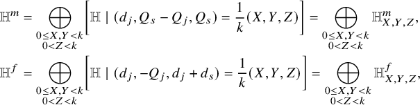 $$ \begin{align*}{\mathbb H}^m&= \bigoplus_{\substack{{0\le X,Y<k}\\{0< Z< k}}} \left[{\mathbb H}\mid (d_j,Q_s-Q_j,Q_s)=\frac1k(X,Y,Z)\right]=\bigoplus_{\substack{{0\le X,Y< k}\\{0< Z<k}}}{\mathbb H}^m_{X,Y,Z} ,\\ {\mathbb H}^f&= \bigoplus_{\substack{{0\le X,Y< k}\\{0< Z< k}}} \left[{\mathbb H}\mid (d_j,-Q_j,d_j+d_s)=\frac1k(X,Y,Z)\right] =\bigoplus_{\substack{{0\le X,Y< k}\\{0< Z< k}}}{\mathbb H}^f_{X,Y,Z},\end{align*} $$
where the choice of the three parameters in  $\{0,\dots , k-1\}$ modulo $k{\mathbb Z}$ are given by
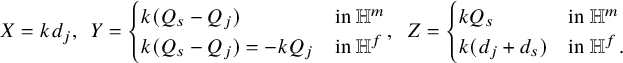 $$ \begin{align} X=kd_j,\ \ Y=\begin{cases}k(Q_s-Q_j)& {\text{in }{\mathbb H}^m}\\ k(Q_s-Q_j)=-kQ_j & {\text{in }{\mathbb H}^f}\end{cases}, \ \ Z =\begin{cases}kQ_s& {\text{in }{\mathbb H}^m}\\ k(d_j+d_s) & {\text{in }{\mathbb H}^f}. \end{cases} \end{align} $$
Note that the definition of Z depends on the sector. These choices are motivated by the following proposition.
Proposition 38 (twist)
For  $Z=1,\dots , k-1$, we have an isomorphism
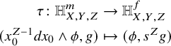 $$ \begin{align*} \tau\colon {\mathbb H}^m_{X,Y,Z}&\to {\mathbb H}^f_{X,Y,Z}\\ (x_0^{Z-1}dx_0\wedge\phi,g)&\mapsto (\phi,s^{Z}g) \end{align*} $$
transforming  $(p,q)$-classes into $(p-1+2Z/k,q)$-classes.
Proof. Indeed, the above homomorphism exchanges  $d_j+d_s$ with $Q_s$ and preserves $d_j$ and $Q_s-Q_j$. Note that $\tau $ only affects the $x_0$ part of W: The fact that $\tau $ is an isomorphism follows from the Thom–Sebastiani principle and the simple description of the state space for $P'=x_0^k.$
There are natural isomorphisms matching  ${\mathbb H}^f_{X,Y,1}\cong {\mathbb H}^f_{X,Y,2}\cong \dots \cong {\mathbb H}^f_{X,Y,k-1}$ and ${\mathbb H}^m_{X,Y,1}\cong {\mathbb H}^m_{X,Y,2}\cong \dots \cong {\mathbb H}^m_{X,Y,k-1}$. We refer to them as ‘elevators’.
Proposition 39 (elevators)
For any  $0\le X,Y< k$ and $0<Z'<Z''<k$, we have the isomorphisms
 $$ \begin{align*} e^m_{Z',Z''}\colon{\mathbb H}^m_{X,Y,Z'}&\to {\mathbb H}^m_{X,Y,Z''}&&&&&e^f_{Z',Z''}\colon{\mathbb H}^f_{X,Y,Z'}&\to {\mathbb H}^f_{X,Y,Z''}\\ (\phi, g)&\mapsto (x_0^{Z''-Z'}\phi, g)&&&&&(\phi, g)&\mapsto (\phi, s^{Z''-Z'}g), \end{align*} $$
with  $e^m_{Z',Z''}$ and $e^f_{Z',Z''}$ transforming $(p,q)$-classes into classes whose bidegrees equal $(p-(Z''-Z')/k,q+(Z''-Z')/k)$ and $(p+(Z''-Z')/k,q+(Z''-Z')/k)$, respectively. □
For  $0<Z'<Z''<k$, we set $e^m_{Z'',Z'}=(e^m_{Z',Z''})^{-1}$ and $e^f_{Z'',Z'}=(e^f_{Z',Z''})^{-1}$.
Proposition 34 specializes to the following statement.
Proposition 40. The mirror isomorphism M yields isomorphisms
 $$ \begin{align*} M\colon {\mathbb H}^f_{X,Y,Z}\xrightarrow{\sim} ({\mathbb H}^{\vee})^m_{Y,X,Z},\qquad \qquad M\colon {\mathbb H}^m_{X,Y,Z}&\xrightarrow{\sim} ({\mathbb H}^{\vee})^f_{Y,X,Z}. \end{align*} $$
Proof. Let us consider M as a morphism mapping  $U_W$ to $U_{W^{\vee }}$. For $W=(x_0)^k+f$, we have $W^{\vee }=((x_0)^k)^{\vee }+f^{\vee }=(x_0)^k+f^{\vee }$. Using equation (21) and Thom–Sebastiani, every state of the form $(\phi ,g)\in U_W$ can be regarded as an element of
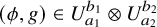 $$ \begin{align*} (\phi,g)\in U^{b_1}_{a_1}\otimes U^{b_2}_{a_2} \end{align*} $$
with  $a_1\in \operatorname {Aut}_{(x_0)^k}={\mathbb Z}/k$, $b_1\in \operatorname {Aut}_{((x_0)^k)^{\vee }}={\mathbb Z}/k$, $a_2\in \operatorname {Aut}_{f}$ and $b_2\in \operatorname {Aut}_{f^{\vee }}.$ Example 30 shows that there are only two possibilities: (1) $b_1$ is the identity element or (2) $a_1$ is the identity element. More precisely, in case (1), $(\phi ,g)$ is in ${\mathbb H}^f$, it is fixed by s, $b_1$ is the trivial symmetry $1\in \operatorname {Aut}_{(x_0)^k}$ and $a_1$ is the nontrivial character corresponding to $kd_s\in {\mathbb Z}/k\setminus \{0\}$. In case (2), $(\phi ,g)$ is in ${\mathbb H}^m$, it is not fixed by s and $a_1$ is trivial whereas $b_1$ is the nontrivial character $kQ_s \in {\mathbb Z}/k\setminus \{0\}$. Since M exchanges $a_1$ and $b_1$, this proves that M exchanges ${\mathbb H}^m$ and ${\mathbb H}^f$ and preserves the coordinate Z which coincides with $kd_s$ and $kQ_s$ within ${\mathbb H}^m$ and ${\mathbb H}^f$.
Furthermore, M maps  $U_{a_2}^{b_2}(f)$ to $U_{b_2}^{a_2}(f^{\vee })$ with $a_2\in \operatorname {SL}_f[j_f]$ and $b_2\in \operatorname {SL}_{f^{\vee }}[j_{f^{\vee }}]$. We recall that $j_f^k\in \operatorname {SL}$ on both sides; therefore, $\det a_2$ and $\det b_2$ are ${\pmb \mu }_k$-characters. The claim $(X,Y,Z)\mapsto (Y,X,Z)$ follows from
 $$ \begin{align*} \det a_2=-kd_j, \qquad \det b_2=-kQ_s+kQ_j, \end{align*} $$
where  ${\pmb \mu }_k$-characters are identified with elements of ${\mathbb Z}/k$. The first identity is immediate: $a_2$ is related to $(\phi ,g)\in U_W$ by $a_2=g\!\mid _{x_0=0}$. The identity follows from $\det (j\!\!\mid _{x_0=0})=\xi _k^{-1}$ by the Calabi–Yau condition. The second identity follows from the definition of
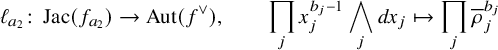 $$ \begin{align*} \ell_{a_2}\colon \operatorname{Jac}(f_{a_2})\to \operatorname{Aut}(f^{\vee}), \qquad \prod_j x_j^{b_j-1}\bigwedge_{j} dx_j\mapsto \prod_j \overline \rho_j^{b_j} \end{align*} $$
from equation (20): The determinant of  $\overline \rho _j$ is $\xi _d^{w_j}$; hence, $\det (\prod _j \overline \rho _j^{b_j})$ is identified with the $j_f$-charge $Q_{j_f}$ of the form $\phi $ restricted to $(x_0=0)$. This yields an identification between $\det b_2$ and the ${\pmb \mu }_k$-character $kQ_j-kQ_s$.
In view of the above proposition, mirror symmetry operates as a plane symmetry exchanging the two blocks; see Figure 1.
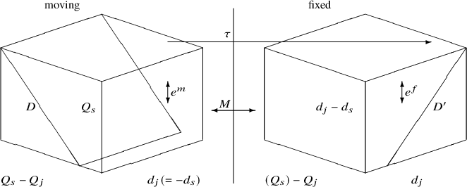
Figure 1 Two blocks (with elevators) representing the coordinates of the moving subspace  ${\mathbb H}^m$ and of the fixed subspace ${\mathbb H}^f$. The condition $Q_j=0$ defines a plane cutting the diagonal D of the left-hand side face of the moving block; D represents the moving part of $H^*_{\operatorname {id}}(\Sigma _{W,H};{\mathbb C})$. On the fixed block, the same condition $Q_j=0$ defines the face on the right-hand side; within it, the diagonal $D'$ is symmetrical to D and represents the fixed part of $H^*_{\operatorname {id}}(\Sigma _{W,H};{\mathbb C})$.
Remark 41. For Fermat potentials, all the above discussion can be carried out more explicitly because the group elements  $\pmb a=\prod _{i=1}^n \rho _i^{a_i}$ coincide with $\frac 1d[a_1w_1,\dots ,a_nw_n]$. By adopting this notation, the space $U_{a}^{b}(W)$ may be regarded as the one-dimensional space spanned by
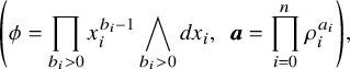 $$ \begin{align*} \left (\phi=\prod_{b_i>0} x_i^{b_i-1} \bigwedge_{b_i>0} dx_i, \ \ \pmb a=\prod_{i=0}^n\rho_i^{a_i}\right), \end{align*} $$
where
 $$ \begin{align} a_i=0 \Leftrightarrow b_i\neq 0. \end{align} $$
Mirror symmetry is simply an exchange of the  $w{\mathbb Z}/d{\mathbb Z}$-valued vectors $\pmb a$ and $\pmb b$. By unravelling Definition 23, the bidegree $(p,q)$ is given by
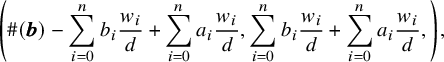 $$ \begin{align*} \left(\#(\pmb b)-\sum_{i=0}^n b_i \frac{w_i}d + \sum_{i=0}^n a_i \frac{w_i}d, \sum_{i=0}^n b_i \frac{w_i}d+ \sum_{i=0}^n a_i \frac{w_i}d,\right), \end{align*} $$
where  $\#(\pmb b)$ is the number of elements i such that $b_i\neq 0$. Notice that $Q_s$ is $b_0/k$ and $d_s+d_j$ is $a_0/k$; therefore, the equivalence in Proposition 37 reads $b_0=0$ is a special case of equation (26). Furthermore, we have
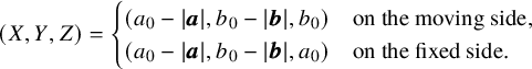 $$ \begin{align*}(X,Y,Z)=\begin{cases} (a_0-|\pmb a|,b_0-|\pmb b|,b_0)&\text {on the moving side,}\\ (a_0-|\pmb a|,b_0-|\pmb b|,a_0)&\text {on the fixed side.} \end{cases} \end{align*} $$
It is now clear that M exchanges the moving side with the fixed side,  $(X,Y,Z)$ with $(Y,X,Z)$ and $(p,q)$ with $(n+1-p,q)$.
In view of Proposition 35, we obtain the j-invariant contribution by setting  $Q_j=0$. By equation (25), this amounts to imposing $Y=Z$ within ${\mathbb H}^m$ and $Y=0$ within ${\mathbb H}^f$. We get
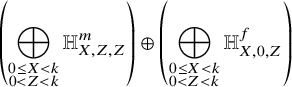 $$ \begin{align*} \left(\bigoplus_{\substack{{0\le X< k}\\{0< Z< k}}} {\mathbb H}^m_{X,Z,Z} \right)\oplus \left(\bigoplus_{\substack{{0\le X< k}\\{0< Z< k}}} {\mathbb H}^f_{X,0,Z} \right) \end{align*} $$
 We get a picture of the j-invariant state space  $\mathcal H_{W,K[j_W],\operatorname {id}}$ by setting $X=0$ within ${\mathbb H}^m$ and $X=Z$ within ${\mathbb H}^f$
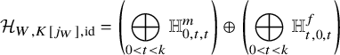 $$ \begin{align*} \mathcal H_{W,K[j_W],\operatorname{id}}=\left(\bigoplus_{\substack{{0< t< k}}} {\mathbb H}^m_{0,t,t} \right)\oplus\left(\bigoplus_{\substack{{0<t< k}}} {\mathbb H}^f_{t,0,t}\right) \end{align*} $$
(we refer to Figure 1). More generally, the  $(d_s=b)$-part of ${\mathbb H}^{j_W}$ is the state space $\mathcal H_{W,K[j_W],s^b}$ (see Proposition 35). By equation (25), we obtain it by setting $X=-b$ within ${\mathbb H}^m$ and $Z=X+b$ within ${\mathbb H}^f$
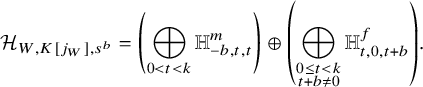 $$ \begin{align} \mathcal H_{W,K[j_W],s^b}=\left(\bigoplus_{\substack{{0< t< k}}} {\mathbb H}^m_{-b,t,t} \right)\oplus\left(\bigoplus_{\substack{{0\le t< k}\\t+b\neq 0}} {\mathbb H}^f_{t,0,t+b}\right). \end{align} $$
Notice that the second summand only depends on  ${\mathbb H}^f_{0,0,1}$ and ${\mathbb H}^f_{1,0,1},\dots {\mathbb H}^f_{k-1,0,k-1}$ since, for $b\neq 0$, it equals
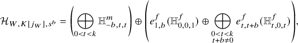 $$ \begin{align} \mathcal H_{W,K[j_W],s^b}= \left(\bigoplus_{\substack{{0< t< k}}} {\mathbb H}^m_{-b,t,t} \right)\oplus\left(e^f_{1,b}({\mathbb H}^f_{0,0,1})\oplus \bigoplus_{\substack{{0< t< k}\\t+b\neq 0}} e^f_{t,t+b}({\mathbb H}^f_{t,0,t})\right), \end{align} $$
with the convention  $(e^f_{i,j})=(e^f_{j,i})^{-1}$ if $j<i$. By Proposition 35, the above data correspond to $H_{s^b}^*(\Sigma _{W,K[j_W]};{\mathbb C})$ under the Calabi–Yau condition.
Proposition 9 relates it to the cohomology of an  $s^b$-fixed locus within a crepant resolution. Using this geometric picture, we can predict some vanishing conditions, which we prove in general, without relying on any Calabi–Yau condition in the next proposition. The first guess is immediate: Since $\langle s\rangle $ operates trivially on an s-fixed locus, it is natural to expect that ${\mathbb H}^m_{-1,t,t}$ vanishes for all t. More generally, since $\langle s^b\rangle $ operates trivially on an $s^b$-fixed locus, we expect that ${\mathbb H}^m_{-b,t,t}$ vanishes if $tb\equiv 0$ mod ${\mathbb Z}$. We prove that this holds true regardless of any Calabi–Yau condition or existence of crepant resolution.
Proposition 42. Let  $b\in \{0,\dots , k-1\}$. We have
 $$ \begin{align*} {\mathbb H}^m_{b,t,t}= 0, \end{align*} $$
unless t is a multiple of  $k/\gcd (b,k)$ in $k{\mathbb Z}$.
Proof. We prove that
 $$ \begin{align*} {\mathbb H}^m_{b,t,t}\neq 0 \end{align*} $$
implies  $bt\in k{\mathbb Z}$. Recall that $\frac {t}k$ equals $Q_s-Q_j$. For ${\mathbb H}^m_{b,t,t}\neq 0$, we can compute $Q_s-Q_j$ explicitly using $(\phi ,j^b g)\in {\mathbb H}^m_{b,t,t}$ with $g\in \operatorname {Aut}_f$ and $\phi $ a g-invariant form
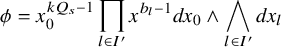 $$ \begin{align*} \phi=x_0^{kQ_s-1}\prod_{l\in I'}x^{b_l-1} dx_0\wedge\bigwedge_{l\in I'}dx_l \end{align*} $$
with  $I'=\{l\ge 1\mid j^b g\cdot x_l=x_l\}\subseteq \{1,\dots , N\}$. Using $w_0/d=1/k$, we get
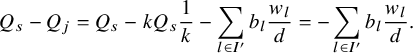 $$ \begin{align*} Q_s-Q_j=Q_s-kQ_s\frac1k-\sum_{l\in I'} b_l\frac{w_l}d=-\sum_{l\in I'} b_l\frac{w_l}d. \end{align*} $$
Let us write g as  $[0,p_1\dots , p_n]\in \operatorname {Aut}_f$; then we have $l\in I'$ if and only if
 $$ \begin{align*} b\frac{w_l}d + p_l\in {\mathbb Z}. \end{align*} $$
Now note that
 $$ \begin{align*} b\frac{t}k = -b\sum_{l\in I} b_l\frac{w_l}d= -\sum_{l\in I} b_l b\frac{w_l}d. \end{align*} $$
Up to an element of  ${\mathbb Z}$, this is
 $$ \begin{align*} \sum_{l\in I} b_l p_l\in {\mathbb Z}, \end{align*} $$
where the last relation holds since  $\phi $ is g-invariant. So k divides $bt$.
$bt$.
6.4 Mirror symmetry on the Landau–Ginzburg side
In this section, we derive an interpretation of Proposition 40 in terms of the Landau–Ginzburg state space. This amounts to expressing both sides of the isomorphism  ${\mathbb H}^m_{X,Y,Z}\cong {\mathbb H}^f_{Y,X,Z}$ in terms of $j_W$-invariant spaces.
Consider the  $j_W$-invariant summands
 $$ \begin{align*} {\mathbb H}^m_{X,Y,Y}\subset {\mathbb H}^m \ \ \text{and}\ \ {\mathbb H}^f_{X,0,Z}\subset {\mathbb H}^f. \end{align*} $$
Their mirrors (i.e., their image under M) are  $({\mathbb H}^{\vee })^f_{Y,X,Y}$ and $({\mathbb H}^{\vee })^m_{0,X,Z}$ and lie in the $j_W$-invariant part if and only if $X=0$ and $X=Z$. This happens if and only if we consider the mirror of $[{\mathbb H}\mid Q_j=d_s=0]$ (imposing $X=0$ in ${\mathbb H}^m$ and $X=Z$ in ${\mathbb H}^f$ is the same as requiring $d_s=0$).
We obtain the first consequence of Proposition 40. Let
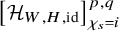 $$ \begin{align*} \left[\mathcal H_{W,H,\operatorname{id}}\right]^{p,q}_{\chi_s=i} \end{align*} $$
be the eigenspace on which s operates as the character  $i\in {\mathbb Z}/k{\mathbb Z}$. For any $H\in \operatorname {Aut}_W$ containing $j_W$, we have
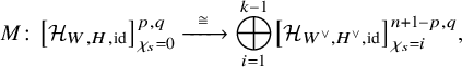 $$ \begin{align} M\colon \left[\mathcal H_{W,H,\operatorname{id}}\right]^{p,q}_{\chi_s=0}\xrightarrow{ \ \ \cong\ \ } \bigoplus_{i=1}^{k-1} \left[\mathcal H_{W^{\vee},H^{\vee},\operatorname{id}}\right]^{n+1-p,q}_{\chi_s=i}, \end{align} $$
where  $H=K[j]$.
We now study  ${\mathbb H}^f_{0,0,i}$. By Proposition 40, the subspace $({\mathbb H}^{\vee })^f_{0,0,i}$ mirrors ${\mathbb H}^m_{0,0,i}$ under M. By applying the twist $\tau $ from Proposition 38, we land again on $({\mathbb H}^{\vee })^f_{0,0,i}$ which is a part of the j-invariant state space $\mathcal H_{W^{\vee },H^{\vee },s^i}$.
Recall that the elevator maps for  $t \neq 0,k-i$
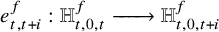 $$ \begin{align*} e^f_{t,t+i}:{\mathbb H}^f_{t,0,t} \xrightarrow{\ \ \ \ \ \ } {\mathbb H}^f_{t,0,t+i} \end{align*} $$
can be viewed as mapping into components of  $\mathcal H_{ W,H,s^i}^s$ (see equation (27)). We can conclude from equation (28) that the homomorphism
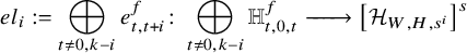 $$ \begin{align} el_i:=\bigoplus_{t\neq 0,k-i} e^f_{t,t+i} \colon \bigoplus_{\substack{{t \neq 0, k-i}}} {\mathbb H}^f_{t,0,t} \xrightarrow{\ \ \ \ \ \ } \left[\mathcal H_{ W,H,s^i}\right]^s \end{align} $$
has cokernel  ${\mathbb H}_{0,0,i}^f$. Here $t+i$ is understood to be mod k. This means that the effect of the map on grading can be described as
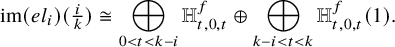 $$\begin{align*}\operatorname{im}(el_i)(\tfrac{i}{k})\cong \bigoplus_{0<t<k-i} {\mathbb H}^f_{t,0,t} \oplus \bigoplus_{k-i<t<k} {\mathbb H}^f_{t,0,t}(1).\end{align*}$$
We write  $el^{\vee }_i$ for the same construction on the mirror. We conclude
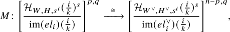 $$ \begin{align} M\colon \left[\frac{\mathcal H_{W,H,s^i}(\tfrac{i}{k})^s}{\operatorname{im}(el_i)(\tfrac{i}{k})}\right]^{p,q} \xrightarrow{\ \ \cong\ \ } \left[\frac{\mathcal H_{W^{\vee},H^{\vee},s^i}(\tfrac{i}{k})^s}{\operatorname{im}(el^{\vee}_i)(\tfrac{i}{k})}\right]^{n-p,q}, \end{align} $$
where the bidegrees have been computed using  $\mathcal H(\frac {i}{k})^{p,q}=\mathcal H^{p+i/k,q+i/k}$, the fact that $M_W$ transforms $(p,q)$-classes to $(n+1-p,q)$-classes and the twist $\tau $ maps $(p,q)$-classes to $(p-1+\frac {2i}{k},q)$-classes.
Note that using equation (29) (recalling that  $d_j$ and $d_s$ switch under mirror symmetry) we can write
 $$\begin{align*}[\operatorname{im}(el^{\vee}_i)(\tfrac{i}{k})]^{n-p,q}= \bigoplus_{0<j<k-i} \left[\mathcal H_{W,H,\operatorname{id}}(1,0)\right]^{p,q}_{\chi_s=j}\oplus \bigoplus_{k-i<j<k} \left[\mathcal H_{W,H,\operatorname{id}}(0,1)\right]^{p,q}_{\chi_s=j}.\end{align*}$$
Write  $\mathcal H_{g}$ for $\mathcal H_{W,H,g}$ and $\mathcal H^{\vee }_g$ for $\mathcal H_{W^{\vee },H^{\vee },g}.$ We obtain
 $$ \begin{align} \begin{aligned} M\colon & [\mathcal H_{s^i}\left(\tfrac{i}{k}\right)]_{\chi_s=0}^{p,q} \oplus \bigoplus_{j<k-i} \left[\mathcal H_{\operatorname{id}}(1,0)\right]^{p,q}_{\chi_s=j}\oplus \bigoplus_{j>k-i} \left[\mathcal H_{\operatorname{id}}(0,1)\right]^{p,q}_{\chi_s=j} \xrightarrow{\ \ \cong\ \ } \\ &\quad [\mathcal H^{\vee}_{s^i}\left(\tfrac{i}{k}\right)]_{\chi_s=0}^{n-p,q} \oplus \bigoplus_{j<k-i} \left[\mathcal H^{\vee}_{\operatorname{id}}(1,0)\right]^{n-p,q}_{\chi_s=j}\oplus \bigoplus_{j>k-i} \left[\mathcal H^{\vee}_{\operatorname{id}}(0,1)\right]^{n-p,q}_{\chi_s=j}, \end{aligned} \end{align} $$
where  $0<j<k.$ Finally, we focus on the moving part of $\mathcal H_{W,K[j_W],s^b}$ which, by equation (28) can be written as $\bigoplus _{0< t< k} {\mathbb H}^m_{k-b,t,t}$. This is the decomposition of $\mathcal H_{W,K[j],s^b}$ into eigenspaces corresponding to the s-action operating as the character $t\in {\mathbb Z}/k$. By applying the mirror map $M_W$, the twist $\tau ^{-1}$ and the elevator $e^f_{t,k-b}$ we get
 $$ \begin{align*} {\mathbb H}^m_{k-b,t,t}\xrightarrow{\ M_W\ } ({\mathbb H}^{\vee})^f_{t,k-b,t}\xrightarrow{\ \tau^{-1}\ } ({\mathbb H}^{\vee})^m_{t,k-b,t}\xrightarrow{\ e^m_{t,k-b}\ } ({\mathbb H}^{\vee})^m_{t,k-b,k-b}. \end{align*} $$
Therefore, we have
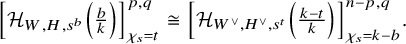 $$ \begin{align} \left[\mathcal H_{W,H,s^b}\left(\textstyle\frac{b}{k}\right)\right]^{p,q}_{\chi_s=t}\cong \left[\mathcal H_{W^{\vee},H^{\vee},s^t}\left(\textstyle\frac{k-t}{k}\right)\right]^{n-p,q}_{\chi_s=k-b}.\end{align} $$
Notice that the map on the bidegrees is the composite of
1. a shift
$(p,q)\mapsto (p+b/k,q+b/k)$,2. mirror symmetry
$(p,q)\mapsto (n+1-p,q)$,3.
$\tau ^{-1}$ yielding $(p,q)\mapsto (p+1-2t/k,q)$,4. the elevator yielding
$(p,q)\mapsto (p+(b-(k-t))/k,q+(b+(k-t))/k)$,5. a shift backwards
$(p,q)\mapsto (p-(k-t)/k,q-(k-t)/k)$,


inducing  $(p,q)\mapsto (n-p,q)$.
We now are almost ready to state the theorem, which will follow from applying equations (29), (32) and (33) to the geometric interpretation (18) of the Landau–Ginzburg state space in terms of relative cohomology of  $({\mathbb V}_H,{\mathbb F}_{W,H})$ (provided in §5.3).
Let  $W=x_0^k+f(x_1,\dots ,x_n)$ be a quasi-homogeneous nondegenerate polynomial of degree d and weights $w_1,\dots ,w_n$. Assume $j_W\in H\subseteq \operatorname {SL}_W$ (in particular, $\sum _j w_j$ is a positive multiple of $d\mathbb N$). Then W descends to ${\mathbb V}_{H}=[{\mathbb V}/H_0]\to {\mathbb C}$ and its generic fibre is ${\mathbb F}_{W,H}$. Consider the automorphism $s=[\frac 1k,0,\dots ,0]\colon {\mathbb V}_H\to {\mathbb V}_H$, the orbifold cohomology groups $H_{\operatorname {id}}^*({\mathbb V}_H,{\mathbb F}_{W,H})$ and $H_{s}^*({\mathbb V}_H,{\mathbb F}_{W,H})$.
For  $0<i<k$, define $\overline {H}^*_{\operatorname {id},i}({\mathbb V}_{H},{\mathbb F}_{W,H})$ to be the bigraded vector space
 $$\begin{align*}\bigoplus_{j<k-i}\left[H^*_{\operatorname{id}}({\mathbb V}_{H},{\mathbb F}_{W,H})\left(1,0\right)\right]_{\chi_s=j} \oplus \bigoplus_{j>k-i}\left[H^*_{\operatorname{id}}({\mathbb V}_{H},{\mathbb F}_{W,H})\left(0,1\right)\right]_{\chi_s=j};\end{align*}$$
here  $j \in \{1,\dots ,k-1\}.$ This is the padding needed to state the mirror theorem.
Theorem 43 (mirror theorem for Landau–Ginzburg models)
Let  $W=x_0^k+f(x_1,\dots ,x_n)$ be a quasi-homogeneous, nondegenerate, invertible polynomial and H a group of symmetries satisfying $j_W\in H\subseteq \operatorname {SL}_W$. As above, the polynomial W descends to ${\mathbb V}_{H}=[{\mathbb V}/H_0]\to {\mathbb C}$, and its generic fibre is ${\mathbb F}_{W,H}$.
Then, for b and  $t\neq 0$, we have
1.
$H^{p,q}_{\operatorname {id}}({\mathbb V}_{H},{\mathbb F}_{W,H})_{\chi _s=0}\cong \bigoplus _{i=1}^{k-1} H^{n+1-p,q}_{\operatorname {id}}({\mathbb V}_{H^{\vee }},{\mathbb F}_{W^{\vee },H^{\vee }})_{\chi _s=i};$2. Let
${\mathbb F}:={\mathbb F}_{W,H}$ and ${\mathbb F}^{\vee }:={\mathbb F}_{W^{\vee },H^{\vee }}$.For
$0<i<k$, $$\begin{align*}\left[H^{p,q}_{s^i}({\mathbb V}_H,{\mathbb F})\left(\tfrac{i}{k} \right)\right]^s \oplus \overline{H}^{p,q}_{\operatorname{id},i}({\mathbb V}_H,{\mathbb F}) \cong \left[H^{n-p,q}_{s^i}({\mathbb V}_{H^{\vee}},{\mathbb F}^{\vee})\left(\tfrac{i}{k}\right)\right]^s \oplus \overline{H}_{\operatorname{id},i}^{n-p,q}({\mathbb V}_{H^{\vee}},{\mathbb F}^{\vee}) ;\end{align*}$$3.
$H^{p,q}_{s^b}({\mathbb V}_{H},{\mathbb F}_{W,H})\left (\frac {b}k\right )_{\chi _s=t}\cong H^{n-p,q}_{s^{-t}}({\mathbb V}_{H^{\vee }},{\mathbb F}_{W^{\vee },H^{\vee }}) \left (\frac {k-t}k\right )_{\chi _s=-b}.$


Proof. Since H equals  $K[j_W]$ for a suitable $K\subseteq \operatorname {SL}_f$ containing $j_W^k$, we can conclude that $\mathcal H _{P,H,g}^{p,q} =H_{g}^{p,q}({\mathbb V}_H;{\mathbb F}_{P,H})$. Using this result, we can translate the results derived above into the form stated in the theorem. More precisely, equation (29) directly gives the first part, equation (32) the second and equation (33) the third.
7 Geometric mirror symmetry
If W is of Calabi–Yau type, via the Landau–Ginzburg/Calabi–Yau correspondence of Theorem 24 based on  $\Phi \colon H^*({\mathbb V};{\mathbb C})\to H^*({\mathbb L};{\mathbb C})$, we provide an equivalent statement on the Calabi–Yau side.
The existence of the isomorphism  $\Phi $ is guaranteed by the Calabi–Yau condition (ensuring K-equivalence). As before, for $0<i<k$, define $\overline {H}^*_{\operatorname {id},i}(\Sigma _{W,H})$ to be the bigraded vector space
 $$ \begin{align} \bigoplus_{j<k-i}\left[H^*_{\operatorname{id}}(\Sigma_{W,H})\left(1,0\right)\right]_{\chi_s=j} \oplus \bigoplus_{j>k-i}\left[H^*_{\operatorname{id}}(\Sigma_{W,H})\left(0,1\right)\right]_{\chi_s=j}, \end{align} $$
where again, j runs between  $1$ and $k-1$. Then we have the following statement.
Theorem 44 (mirror theorem for CY orbifolds with automorphism s)
Let  $W=x_0^k+f(x_1,\dots ,x_n)$ be a be a quasi-homogeneous, nondegenerate, invertible, Calabi–Yau polynomial and H a group of symmetries satisfying $j_W\in H\subseteq \operatorname {SL}_W$. Let $\Sigma =\Sigma _{W,H}$ and $\Sigma ^{\vee }=\Sigma _{W^{\vee },H^{\vee }}.$ Then the following holds for $b,t\neq 0$.
1. Let
$d=n-1$. Then $H^{p,q}_{\operatorname {id}}(\Sigma )_{\chi _s=0}\cong \bigoplus _{i=1}^{k-1} H^{d-p,q}_{\operatorname {id}}(\Sigma ^{\vee })_{\chi _s=i};$2. Let
$d=n-2$. For $0<i<k$, $$ \begin{align*} \left[H^{p,q}_{s^i}(\Sigma)\left(\tfrac{i}{k}\right)\right]^s \oplus \overline{H}^{p,q}_{\operatorname{id},i}(\Sigma)\cong \left[H^{d-p,q}_{s^i}(\Sigma^{\vee})\left(\tfrac{i}{k}\right)\right]^s \oplus \overline{H}_{\operatorname{id},i}^{d-p,q}(\Sigma^{\vee});\end{align*} $$3. Let
$d=n-2$. Then $H^{p,q}_{s^b}(\Sigma )_{\chi _s=t}\left (\frac {b}k\right )\cong H^{d-p,q}_{s^{-t}}(\Sigma ^{\vee })\left (\frac {k-t}k\right )_{\chi _s=-b}.$


Remark 45. In the theorem, d denotes the maximum of the dimensions of the components of the inertia stack considered in each case.
For  $k=2$, the second equation of the statement of Theorem 44 can be stated as a mirror symmetry statement involving the cohomology groups $H^{*}_s$. Notice that the first statement says that Berglund–Hübsch mirror symmetry exchanges invariant $(p,q)$-classes for $\Sigma _{W,H}$ and anti-invariant $(n-1-p,q)$-classes of $\Sigma _{W^{\vee },H^{\vee }}$ (and vice versa). Finally, the third statement is trivial because both sides vanish by Proposition 42. In this way, we recover the main theorem of [Reference Chiodo, Kalashnikov and Veniani12].
Corollary 46. Let  $W=x_0^2+f(x_1,\dots ,x_n)$ be a be a quasi-homogeneous, nondegenerate, invertible, Calabi–Yau polynomial and H a group of symmetries satisfying $j_W\in H\subseteq \operatorname {SL}_W$. Then, we have
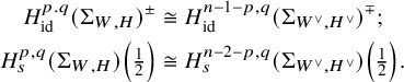 $$ \begin{align*} H^{p.q}_{\operatorname{id}}(\Sigma_{W,H})^{\pm}&\cong H^{n-1-p,q}_{\operatorname{id}}(\Sigma_{W^{\vee},H^{\vee}})^{\mp};\\ H^{p,q}_s(\Sigma_{W,H})\textstyle{\left(\frac{1}2\right)}&\cong H^{n-2-p,q}_s(\Sigma_{W^{\vee},H^{\vee}})\textstyle{\left(\frac{1}2\right)}.\end{align*} $$
Example 47. Let us consider  $E=(x^6+y^3+z^2=0)$ within ${\mathbb P}(1,2,3)$ with its order- $6$ symmetry $s=[\frac 16,0,0]$. In this case, the ‘Calabi–Yau orbifold’ is represented by an elliptic curve. The cohomology groups $H_{s^b}^*$ describe the cohomology of the $s^b$-fixed loci $E_b$, shifted by $(\frac {b}6,\frac {b}6)$. Furthermore, the mirror of E coincides with E because the defining equation is of Fermat type and J equals $\operatorname {SL}$ (the order of $\operatorname {SL}$ is $w_xw_yw_z/\deg $ and equals the order $\deg $ of J). This example allows us to test ${\mathbb H}$ as a state space computing the cohomology of E and the cohomology of its fixed spaces satisfying $E_1=E_{2}\cap E_{3}$ and $E_{2}=E_{4}$. Since E is the elliptic curve with order- $6$ complex multiplication, $E_1$ is the origin and the fixed spaces $E_{3}(=E[2])$ and $E_{2}$ are, respectively, a set of four points and three points intersecting at the origin. Clearly, $E_{3}\setminus E_1$ is the unique order- $3$ orbit and $E_{2}\setminus E_1$ is the unique order- $2$ orbit.
The bth row in the table below represents the ranks of contributions of  ${\mathbb H}[d_s=\frac {b}6]$, whereas the ath column represents the contributions to the state space of ${\mathbb H}[d_j=\frac {a}6]$. Notice that, by means of the elevators, all rows are identical except for the antidiagonal entries of the form ${\mathbb H}[d_j+d_s=0]$, which we underlined.
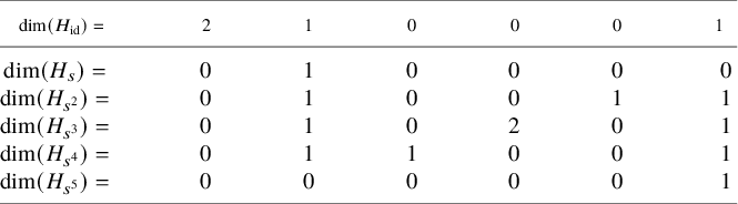
The  $0$th row is the four-dimensional cohomology of the elliptic curve E organised in its two-dimensional primitive part (spanned by the forms $dx\wedge dy\wedge dz$ and $x^4ydx\wedge dy\wedge dz$) and its two-dimensional ambient part arising in the state space ${\mathbb H}[d_s=0, d_j=a/6]$ for $a=1$ and $a=5$ (j and $j^5$ correspond to the only narrow sectors of the state space, i.e., the only powers of $[\frac 16,\frac 13,\frac 12]$ fixing only the origin). On the row corresponding to $H^*_s$, there is a single contribution for $d_j=1/5$. This happens because $E_1$ is a point. Furthermore, ${\mathbb H}[d_j=5/6, d_s=1/6]={\mathbb H}[d_j=1/6, d_s=5/6]$ vanish by Proposition 42. The remaining antidiagonal terms are ${\mathbb H}[d_j=4/6, d_s=2/6]={\mathbb H}[d_j=2/6, d_s=4/6]= \langle x^2dx\wedge dz\rangle $ and ${\mathbb H}[d_j=3/3, d_s=3/3]=\langle xydx\wedge dy,x^3dx\wedge dy\rangle $.
The above mirror symmetry statement (1) involves the first row and claims that all fixed cohomology classes appearing for  $d_j=\frac 16,\dots ,\frac 56$ match the classes of ${\mathbb H}[d_j=0, d_s=0]$; we already noticed that this identifies two two-dimensional spaces of ambient and primitive cohomology. Statement (2), for $i=1$, says that the one-dimensional space ${\mathbb H}[d_s=0, q_j=1,2,3,4]$ (spanned by the class $dx\wedge dy\wedge dz$) matches the cohomology class spanned by $x^4 dx \wedge dy \wedge dz$.
Statement (3) is a map  $M\colon xydx\wedge dy\mapsto x^2dx\wedge dz\in {\mathbb H}[d_j=\frac 26, d_s=\frac 46]$ and a map $M\colon x^3dx\wedge dy\mapsto x^2dx\wedge dz\in {\mathbb H}[d_j=\frac 46, d_s=\frac 26]$. In this way,
 $$ \begin{align*} M\colon {\mathbb H}\left[d_j=\frac36, d_s=\frac36\right]\xrightarrow {\ \ \ \cong\ \ \ }{\mathbb H}\left[d_j=\frac26, d_s=\frac46\right]\oplus {\mathbb H}\left[d_j=\frac46, d_s=\frac26\right]. \end{align*} $$
In geometric terms, mirror symmetry matches the order- $2$ orbit to the order- $3$ orbit. More precisely, the mirror statement (3) claims that there are as many eigenvectors of eigenvalue $(\chi _6)^2$ and $(\chi _6)^4$ in the cohomology of $E_{3}$ as eigenvectors of eigenvalue $(\chi _6)^3$ in the cohomology of $E_{2}$ and of $E_{4}$.
Example 48. We consider the genus- $3$ curve C defined by the degree- $4$ Fermat quartic $x_1^4+x_2^4+x_3^4=0$ in ${\mathbb P}^2$. The $4$-fold cover of ${\mathbb P}^2$ ramified on C is a K3 surface defined as the vanishing locus of the polynomial $W=x_0^4+x_1^4+x_2^4+x_3^4$. In this example, the Calabi–Yau orbifold $\Sigma _{W}$ is again representable and we can treat the cohomologies $H_{\operatorname {id}}^*$ and $H_s^*$ as ordinary cohomologies of the K3 surface and of the ramification locus. As in the previous example, we display the cohomological data in a table. The bth row in the table below represents the ranks of contributions of ${\mathbb H}[d_s=\frac {b}4]$, whereas the ath column represents the contributions to the state space of ${\mathbb H}[d_j=\frac {a}4]$.
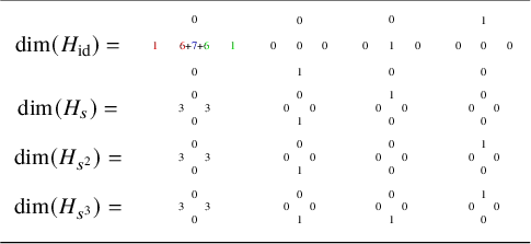
The colors in the table refer to the weight of s: Cohomology in red has character  $1$, blue has character $2$ and green has character $3$. Statement (2) involves, on one side, the cohomology of the curve C ( $H_s$) and the moving cohomology of the K3 surface with weights $1$ and $2$. The total cohomology on one side of statement (2) is thus
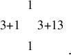
We notice that the only  $\operatorname {SL}$-invariant broad cohomology classes in the entire unprojected state space $U(W)$ are contained in $U(W)_{\operatorname {id}}$; this implies $U(W)_{sg}^{\operatorname {SL}}=0$. Hence, $ H^*_{\mathrm {prim},s}$ vanishes. One can compute the mirror table as
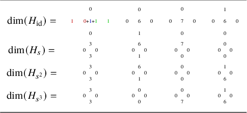
From this, we see that the mirror s-fixed locus is four projective curves and 12 isolated fixed points. The mirror Hodge diamond for statement (2) is

Note that despite being an order-2 automorphism, the Hodge diamonds of the fixed loci of  $s^2$ do not mirror each other.
Clearly, mirror symmetry should also yield a relation between the quantum invariants of the primitive classes of the curve and the orbifold quantum invariants of these sectors.
The structure of the of the above example is shared by all K3 orbifolds of this type with order-4 automorphism. Combining the mirror theorem with the fact that s and  $s^3$ have the same fixed locus (and hence cohomology of the same dimension), we can see that, for any $W=x_0^4+f(x_1,x_2,x_3)$ and group G, the table for $\Sigma _{W,G}$ is given by
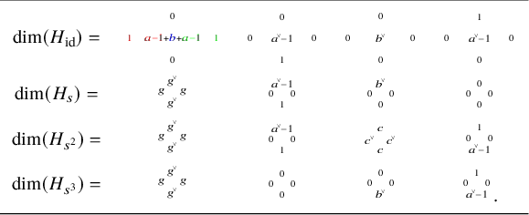
The table for the  $\Sigma _{W^{\vee },G^{\vee }}$ is obtained from this table by replacing $x \mapsto x^{\vee }.$
Using this table, we can find relationships between the topological invariants of the fixed loci of crepant resolutions of  ${\mathfrak X}:=\Sigma _{W,G}$ and its mirror ${\mathfrak X}^{\vee }$. Example 11 shows that there is an isomorphism between the $s^{3}$-orbifold cohomology of ${\mathfrak X}$ and the cohomology of the s fixed locus in the resolution $\widetilde X$. Recall that this is because for K3 surfaces, the age function is constant (of $3/4$) on the $s^3$-orbifold cohomology of the resolution. By similar reasoning, the $s^2$-orbifold cohomology of $\widetilde X$ also has a constant age function (of $1/2$).
Now consider the following invariants for  $i=1,2$:
•
$f_i,$ the number of isolated fixed points of $s^i$;•
$g_i,$ the sum of the genera of the fixed curves of $s^i$;•
$N_i,$ the number of curves in the fixed locus of $s^i$.


A superscript  $\vee $ indicates the invariants of the mirror K3.
Corollary 49. We have
1.
$N_1=g_1^{\vee }+1$;2.
$N_2+g_2+f_1=20-N_2^{\vee }-g_2^{\vee }-f_1^{\vee }.$


Proof. The table above implies that  $2a+b+2a^{\vee }+b^{\vee }=24$ and that $g_1=g$, $N_1=g^{\vee }+1$, and $f_1=a^{\vee }+b^{\vee }-2$. The statements for the mirror invariants are obtained by $x \leftrightarrow x^{\vee }$: For example, $N_1^{\vee }= g+1.$
Similarly,  $N_2-g_2^{\vee }=(g^{\vee }+c+a^{\vee })-(g^{\vee }+c)=a^{\vee }$, which implies the statement.
The same analysis also works for K3 surfaces with prime order automorphisms. Let W be a Calabi–Yau polynomial of the form  $W=x_0^p+f(x_1,x_2,x_3)$ for p prime. Then the Landau–Ginzburg state space breaks down as
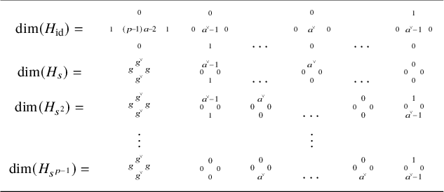
The following lemma follows immediately from considering this table.
Lemma 50. Suppose  $\Sigma _{W,H}$ is a K3 orbifold with $W=x_0^p +f(x_1,x_2,x_3)$. Then $p-1 | 24.$
Let  $\tilde {X}$ be a crepant resolution of ${\mathfrak X}=\Sigma (W,G)$ and $\tilde {X}^{\vee }$ a crepant resolution of the mirror. The fixed locus of s is a disjoint union of curves an isolated fixed points. As before, let $f_1$ be the number of isolated fixed points, $N_1$ the number of curves, and $g_1$ the sum of the genera of the curves.
Corollary 51. Suppose  $p>2$. Then $N_1=g_1^{\vee }+1$ and
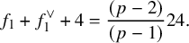 $$ \begin{align*} f_1+f_1^{\vee}+4=\frac{(p-2)}{(p-1)} 24. \end{align*} $$
Proof. Using the table, it is easy to see
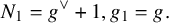 $$ \begin{align*} N_1=g^{\vee}+1, g_1=g. \end{align*} $$
Additionally,
 $$ \begin{align*} f_1=(p-2)a^{\vee}-2. \end{align*} $$
Combining this with  $(p-1)a+(p-1)a^{\vee }=24$, we obtain the statement in the theorem.
This corollary implies that Berglund–Hübsch mirror symmetry agrees with mirror symmetry for lattice polarised K3 surfaces. We briefly recall the latter.
Given a smooth K3 surface  $\Sigma $, $\Lambda =H^2(\Sigma ,{\mathbb Z})$ is equipped with a lattice structure via the cup product taking values in $H^4(\Sigma ;{\mathbb Z})={\mathbb Z}.$ Let $S_{\Sigma }:=\Lambda \cap H^{1,1}(\Sigma; {\mathbb C})$ be the Picard lattice of $\Sigma $.
Let M be a hyperbolic lattice with signature  $(1,t-1)$. A K3 surface $\Sigma $ is called M-polarized if there exists a primitive embedding $M \hookrightarrow S_{\Sigma }$. Given a nonsymplectic automorphism s of $\Sigma $, the invariant sublattice $S(s):=\Lambda ^s$ is in fact a primitive sublattice of the Picard lattice.
Definition 52. Given M a primitive hyperbolic sublattice of  $\Lambda =H^2(\Sigma ,{\mathbb Z})$ of rank at most 19 such that
 $$ \begin{align*} M^{\perp}=U \oplus M^{\vee}, \end{align*} $$ $M^{\vee }$ is defined to be the mirror lattice to M.
Recall that we have restricted to the case where s has prime order  $p>2$ (we have discussed $p=2$ in [Reference Chiodo, Kalashnikov and Veniani12]). We now show that if two K3 surfaces with prime order automorphisms arise as crepant resolutions of a mirror pair of Berglund–Hübsch orbifolds, they have mirror lattices. In this case, $M:=S(s)$ is p-elementary. That is, $M^*/M =({\mathbb Z}/p {\mathbb Z})^{\oplus a}$, and it is completely classified by its rank r and a. Then, by [Reference Artebani, Sarti and Taki3], the fixed locus of s is either just isolated points or a disjoint union of N curves, of which $N-1$ are rational and the remaining one has genus g and f isolated points. Set $m=\frac {22-r}{p-1}$. Moreover, [Reference Artebani, Sarti and Taki3] states (in a slightly different form) that, for $p=3,5,7,13$, if the fixed locus contains a curve,
•
$m=2g+a, -g+N=\frac {r-11+p}{p-1}.$

Notice that these are the only prime orders we need to consider as we have shown that  $p-1 | 24$.
Lattice mirror symmetry exchanges  $(r,a)$ with $(20-r,a)$.
Theorem 53. Let  $\Sigma _{W,H}$ and $\Sigma _{W^{\vee },H^{\vee }}$ be mirror K3 orbifolds with prime order $p>2$ automorphisms $s, s^{\vee }$, and let $\Sigma $ and $\Sigma ^{\vee }$ be crepant resolutions with automorphisms also denoted $s, s^{\vee }$. Then $\Sigma $ and $\Sigma ^{\vee }$ are mirror as lattice polarized K3 surfaces.
Proof. Corollary 51 relates the invariants  $(g,N,f)$ and $(g^{\vee },N^{\vee },f^{\vee })$. It is enough to show that these relations give the mirror relations on $(r,a)$, namely that
 $$ \begin{align*} (r^{\vee},a^{\vee})=(20-r,a). \end{align*} $$
Notice that there is always a fixed curve when the K3 is a hypersurface in weighted projective space of this form. Therefore, we see that
 $$ \begin{align*} r^{\vee}=(-g^{\vee}+N^{\vee})(p-1)&+(11-p)=(-N+g+2)(p-1)+(11-p)\\ &=(p-1)(2-\frac{r-11+p}{p-1})+11-p=20-r. \end{align*} $$
Finally, this implies
 $$ \begin{align*} a^{\vee}=2g^{\vee}-\frac{22-r^{\vee}}{p-1}=2(N-1)-\frac{2+r}{p-1}. \end{align*} $$
Using that  $N=\frac {r-11+p}{p-1}+g,$ we obtain that
 $$ \begin{align*} a^{\vee}=2g-\frac{22-r}{p-1}=a.\\[-36pt] \end{align*} $$
Acknowledgements
Alessandro Chiodo is supported by the ANR project ‘Categorification in Algebraic Geometry’, CANR-17-CE40-0014 and the ANR project ‘Enumerative Geometry’, PRC ENUMGEOM. Elana Kalashnikov is supported by Discovery Grant RGPIN-2022-03013 from the Natural Sciences and Engineering Research Council of Canada.
Conflicts of Interest
none


 Open access