


1 Introduction
The performance of a first-stage liquid propellant rocket engine is highly dependent on the behaviour of the flow as it expands through a supersonic nozzle. Given the mechanical power that is required for an Earth-to-orbit first stage to achieve mission-average specific impulse, large area ratios are desired. Therefore, because the flow is overexpanded at sea-level launch conditions, the structural design of the nozzle wall is driven by the maximum allowable buckling loads that form during startup. That is, the pressure ratio during startup is below the design pressure ratio of the nozzle, which causes the expanding gas to separate from the nozzle wall. High-area-ratio nozzles with wall-separated flows are incubators for shock wave–boundary layer interactions (SWBLI), thermal and material stresses and a turbulent recirculation zone. These complicated flow and shock patterns produce off-axis side loads, which couple with the nozzle to produce fluid–structure interactions with sufficient strength to cause structural failure of the nozzle (Nave & Coffey Reference Nave and Coffey1973). Many independent investigations (Chen, Chakravarthy & Hung Reference Chen, Chakravarthy and Hung1994; Nasuti & Onofri Reference Nasuti and Onofri1998; Hagemann, Frey & Koschel Reference Hagemann, Frey and Koschel2002; Ostlund Reference Ostlund2002) have identified the existence of two kinds of separated nozzle flow regimes. There are free shock separation (FSS) and restricted shock separation (RSS); a review of the literature describing these kinds of flow states is provided by Hadjadj & Onofri (Reference Hadjadj and Onofri2009). Thus, an understanding of the loads produced by these different flow separation regimes is paramount to the safety and reliability of current and future rocket launch systems.
The type of shock pattern (FSS or RSS) that forms inside the nozzle is dependent on the shape of the nozzle wall and the nozzle pressure ratio (NPR; ratio of plenum pressure $p_{0}$
to ambient pressure
$p_{0}$
to ambient pressure $p_{a}$
). Truncated ideal contour (TIC) nozzles display only the FSS type, which is shown in figure 1(a). For FSS flow, an adverse pressure gradient forms along the nozzle wall that causes the flow to separate, resulting in the consequent formation of compression waves that coalesce to form a conical separation shock. In conical nozzles, shock-induced separation occurs when the ratio of the wall pressure and the ambient pressure is between 0.2 and 0.4, depending on the design Mach number (Stark Reference Stark2013). In figure 1(a), reflection of the separation shock on the nozzle axis of symmetry is shown to produce a Mach disk and a second oblique leg (reflected shock). These three shocks meet at the so-called triple point. This type of interaction is named free since the separated shear layer never reattaches to the nozzle wall. In thrust optimized contour (TOC) and thrust optimized parabolic (TOP) nozzles, as the NPR increases, the flow transitions from FSS flow to RSS flow; the pressure ratio that governs the FSS to RSS transition is unique to each nozzle contour. Figure 1(b) identifies the general features of RSS flow, which is characterized by a cap-shock pattern (Nave & Coffey Reference Nave and Coffey1973) and the reattachment of the separated shear layer to the wall with a large recirculation bubble (not shown in the figure) on the nozzle centreline (Nasuti & Onofri Reference Nasuti and Onofri1998).
$p_{a}$
). Truncated ideal contour (TIC) nozzles display only the FSS type, which is shown in figure 1(a). For FSS flow, an adverse pressure gradient forms along the nozzle wall that causes the flow to separate, resulting in the consequent formation of compression waves that coalesce to form a conical separation shock. In conical nozzles, shock-induced separation occurs when the ratio of the wall pressure and the ambient pressure is between 0.2 and 0.4, depending on the design Mach number (Stark Reference Stark2013). In figure 1(a), reflection of the separation shock on the nozzle axis of symmetry is shown to produce a Mach disk and a second oblique leg (reflected shock). These three shocks meet at the so-called triple point. This type of interaction is named free since the separated shear layer never reattaches to the nozzle wall. In thrust optimized contour (TOC) and thrust optimized parabolic (TOP) nozzles, as the NPR increases, the flow transitions from FSS flow to RSS flow; the pressure ratio that governs the FSS to RSS transition is unique to each nozzle contour. Figure 1(b) identifies the general features of RSS flow, which is characterized by a cap-shock pattern (Nave & Coffey Reference Nave and Coffey1973) and the reattachment of the separated shear layer to the wall with a large recirculation bubble (not shown in the figure) on the nozzle centreline (Nasuti & Onofri Reference Nasuti and Onofri1998).

Figure 1. Schematic of the two common flow regimes that form inside the diverging section of high-area-ratio supersonic nozzles. (a) Free shock separation flow found in TIC, TOC and TOP nozzles. (b) Restricted shock separation flow found in TOC and TOP nozzles.
The earliest reports on nozzle side loads proposed that oscillations of the internal shock system inside the nozzle were the main drivers for off-axis side loads. For TOP and TOC nozzles, side loads peak when the flow undergoes FSS to RSS transition (Frey & Hagemann Reference Frey and Hagemann2000; Ostlund Reference Ostlund2002). Earlier efforts turned towards developing analytical and empirical tools capable of predicting the occurrence of side loads based on statistical models of the shock motion. For example, Schmucker (Reference Schmucker1984) developed a model based on the idea of a tilted separation line, while Dumnov (Reference Dumnov1996) considered oscillations of the separation line excited by random pressure pulsations in the separated flow region. These methods rely on many simplifications and are primarily tailored for use as design tools. As both numerical and experimental disciplines have made numerous advances in the past two decades, the focus is being directed towards developing a more physical understanding of the underlying mechanisms responsible for these lateral forces.
The present work focuses on the FSS pattern, which is common to all supersonic nozzles and is characterized by intense side-load activity (Ruf, McDaniels & Brown Reference Ruf, McDaniels and Brown2010). Numerous efforts have been made to characterize the unsteady wall pressure during FSS flow. In particular, Baars et al. (Reference Baars, Tinney, Ruf, Brown and McDaniels2012) and Baars & Tinney (Reference Baars and Tinney2013) showed that the unsteady wall pressure of a cold-gas, subscale parabolic nozzle during FSS flow is characterized by broad low- and high-frequency peaks associated with SWBLI and turbulent shear layer development, respectively. Those authors were able to isolate the effect of the asymmetric azimuthal mode, which is the mode responsible for generating side loads. More recently, Jaunet et al. (Reference Jaunet, Arbos, Lehnasch and Girard2017) observed the evolution of the FSS pattern and the associated Fourier azimuthal modes by varying NPR in a subscale TIC nozzle. They showed how low-frequency fluctuations in the pressure field are primarily asymmetric and are confined to the interior regions of the nozzle. However, the developing turbulent shear layer was shown to comprise high-frequency signatures in the pressure and velocity fields and were observed both inside and outside of the nozzle. Jaunet et al. (Reference Jaunet, Arbos, Lehnasch and Girard2017) also found highly organized pressure structures at an intermediate-frequency range, mainly associated with the asymmetric pressure mode, and argued that the structures were attributed to a screech-like mechanism (Raman Reference Raman1999; Edgington-Mitchell Reference Edgington-Mitchell2019) as opposed to transonic resonance (Wong Reference Wong2005).
Experimental efforts seem to suggest that the various frequency and azimuthal modes inside the nozzle are general features of the FSS pattern. However, experiments on axisymmetric nozzles suffer from the lack of flow measurements inside the nozzle itself, due to the challenging flow conditions and limited optical access. Therefore, numerical simulations can be leveraged as a complementary tool to gain insight into the internal flow physics of separated rocket nozzle flows, and to provide a pathway for addressing important outstanding questions. Of particular interest is a desire to better understand the kinds of frequencies and flow modes that characterize the vortices in the initial part of the supersonic shear layer. Furthermore, if a screech-like mechanism is present due to the interaction of the turbulent shear layer and the shock cell inside the jet, then it is of interest to understand the role of the Mack disk and subsonic flow region in the feedback loop.
Unsteady Reynolds-averaged Navier–Stokes (RANS) equations have been used in the past to evaluate the side loads produced by subscale models, and with rather accurate results being obtained (Deck & Guillen Reference Deck and Guillen2002; Deck & Nguyen Reference Deck and Nguyen2004). However, modelling the global effect of the turbulent scales, as done in the unsteady RANS approach, could mask some of the important features relevant to the formation of unsteady aerodynamic loads. On the other hand, a direct numerical simulation of this kind of flow, characterized by Reynolds numbers of the order of $10^{7}$
, is impractical given the extremely high computational expense. The same is true for a wall-resolved large-eddy simulation (LES). Therefore, a practical alternative to unsteady RANS equations, direct numerical simulation and LES is the use of the detached eddy simulation (DES) method described by Spalart et al. (Reference Spalart, Jou, Strelets and Allmaras1997). The DES method comprises a hybrid of RANS and LES methods and allows high-Reynolds-number flows comprising massive flow separation to be modelled. In fact, in the DES approach, attached boundary layers are treated in RANS mode (thus lowering the computational requirements), while the most energetic turbulent scales of the separated shear layers and turbulent recirculating zones are treated directly in LES mode. As shown by a series of recent studies (Martelli et al.
Reference Martelli, Ciottoli, Bernardini, Nasuti and Valorani2017, Reference Martelli, Ciottoli, Saccoccio, Nasuti, Valorani and Bernardini2019; Memmolo, Bernardini & Pirozzoli Reference Memmolo, Bernardini and Pirozzoli2018), the DES method has proven to be a powerful tool for investigating the flow physics of SWBLI involving massive flow separation where the dynamics is mainly characterized by the dominance of downstream effects (Clemens & Narayanaswamy Reference Clemens and Narayanaswamy2014; Estruch-Samper & Chandola Reference Estruch-Samper and Chandola2018). However, very few DES simulations of separated rocket nozzle flows are discussed in the open literature. Deck (Reference Deck2009) and Shams et al. (Reference Shams, Lehnasch, Comte, Deniau and Alziary de Roquefort2013) presented a delayed DES (DDES) of the end-effect regime in an axisymmetric nozzle flow characterized by RSS. While the simulation reproduced the main flow properties rather well, the most energetic frequency, as predicted by the simulation, was higher than that observed in the experiment. As far as FSS is concerned, to the best of the authors’ knowledge, the only DES available has been reported by Larusson, Andersson & Ostlund (Reference Larusson, Andersson and Ostlund2016), who exclusively focused on the prediction of the side-load magnitude.
$10^{7}$
, is impractical given the extremely high computational expense. The same is true for a wall-resolved large-eddy simulation (LES). Therefore, a practical alternative to unsteady RANS equations, direct numerical simulation and LES is the use of the detached eddy simulation (DES) method described by Spalart et al. (Reference Spalart, Jou, Strelets and Allmaras1997). The DES method comprises a hybrid of RANS and LES methods and allows high-Reynolds-number flows comprising massive flow separation to be modelled. In fact, in the DES approach, attached boundary layers are treated in RANS mode (thus lowering the computational requirements), while the most energetic turbulent scales of the separated shear layers and turbulent recirculating zones are treated directly in LES mode. As shown by a series of recent studies (Martelli et al.
Reference Martelli, Ciottoli, Bernardini, Nasuti and Valorani2017, Reference Martelli, Ciottoli, Saccoccio, Nasuti, Valorani and Bernardini2019; Memmolo, Bernardini & Pirozzoli Reference Memmolo, Bernardini and Pirozzoli2018), the DES method has proven to be a powerful tool for investigating the flow physics of SWBLI involving massive flow separation where the dynamics is mainly characterized by the dominance of downstream effects (Clemens & Narayanaswamy Reference Clemens and Narayanaswamy2014; Estruch-Samper & Chandola Reference Estruch-Samper and Chandola2018). However, very few DES simulations of separated rocket nozzle flows are discussed in the open literature. Deck (Reference Deck2009) and Shams et al. (Reference Shams, Lehnasch, Comte, Deniau and Alziary de Roquefort2013) presented a delayed DES (DDES) of the end-effect regime in an axisymmetric nozzle flow characterized by RSS. While the simulation reproduced the main flow properties rather well, the most energetic frequency, as predicted by the simulation, was higher than that observed in the experiment. As far as FSS is concerned, to the best of the authors’ knowledge, the only DES available has been reported by Larusson, Andersson & Ostlund (Reference Larusson, Andersson and Ostlund2016), who exclusively focused on the prediction of the side-load magnitude.
In this study, we present the results of a DES of a TIC nozzle with flow separation. The geometry has been tested at the University of Texas at Austin, where measurements of the unsteady wall-pressure signatures were recorded. The analysis focuses first on the behaviour of these wall-pressure signatures and on elucidating the underlying mechanisms responsible for generating aerodynamic loads. Numerical results are then used to investigate and characterize parts of the flow not easily accessible using conventional experiment instruments. These are the Mach disk region and the initial part of the annular supersonic shear layer.
The article is organized as follows. First, a description of the experimental apparatus and instrumentation is provided in § 2 followed by an overview of the DDES approach, the numerical solver and the computational set-up in § 3. The first set of results from the DDES model are then discussed in § 4 with an emphasis on the general features of the flow that forms inside a TIC nozzle. In § 5, the main features of the wall-pressure signatures are analysed by way of space–time correlations and spectral analysis. Section 6 focuses on a discussion of the dynamics of the annular shear layer and Mach disk, which play a key role in the existence of an aeroacoustic feedback loop, which we propose and discuss in § 7. A summary of the effort and conclusions are finally given in § 8.
2 Main features of the experimental campaign
2.1 Facility and nozzle test article
The reduced-scale nozzle studied here has a TIC and was designed by the Nozzle Test Facility team at NASA Marshall Space Flight Center (Ruf, McDaniels & Brown Reference Ruf, McDaniels and Brown2009). An illustration of the nozzle contour is shown in figure 2(a) and comprises a throat radius of $r_{t}=19.0$
mm, an exit radius of
$r_{t}=19.0$
mm, an exit radius of $r_{e}=117.43$
mm and a throat-to-exit length of
$r_{e}=117.43$
mm and a throat-to-exit length of $L=350.52$
mm. The nozzle’s exit-to-throat area ratio of
$L=350.52$
mm. The nozzle’s exit-to-throat area ratio of $A_{e}/A^{\ast }=38$
results in a design exit Mach number of
$A_{e}/A^{\ast }=38$
results in a design exit Mach number of $M_{d}=5.58$
at a NPR of 970. The length of the diverging nozzle contour is 79% of a 15
$M_{d}=5.58$
at a NPR of 970. The length of the diverging nozzle contour is 79% of a 15 $^{\circ }$
conical nozzle with the same area ratio and is a standard truncation length for TIC nozzles (Rao Reference Rao1958).
$^{\circ }$
conical nozzle with the same area ratio and is a standard truncation length for TIC nozzles (Rao Reference Rao1958).

Figure 2. (a) Schematic of the nozzle with coordinate system. (b) The TIC nozzle contour identifying the axial locations of the static and dynamic pressure ports.
All measurements were acquired in a fully anechoic chamber at the University of Texas at Austin. The chamber walls are treated with sound-absorbing material with a normal incidence sound absorption coefficient of 99 % above 100 Hz in order to minimize acoustic reflections from exciting the shear layer and internal flow. Interior dimensions (from wedge tip to wedge tip) are $5.8~\text{m}$
(length)
$5.8~\text{m}$
(length) $\times \,4.6~\text{m}$
(width)
$\times \,4.6~\text{m}$
(width) $\times \,3.7~\text{m}$
(height) with the nozzle centreline coinciding with the centreline of the chamber. Behind the nozzle is a
$\times \,3.7~\text{m}$
(height) with the nozzle centreline coinciding with the centreline of the chamber. Behind the nozzle is a $1.22~\text{m}\times 1.22~\text{m}$
opening that supplies ambient air to the chamber that then exhausts through a
$1.22~\text{m}\times 1.22~\text{m}$
opening that supplies ambient air to the chamber that then exhausts through a $1.83~\text{m}\times 1.83~\text{m}$
acoustically treated duct. Additional details of the facility, test article and data acquisition system are provided by Baars & Tinney (Reference Baars and Tinney2013), Baars et al. (Reference Baars, Tinney, Wochner and Hamilton2014) and Donald et al. (Reference Donald, Baars, Tinney and Ruf2014).
$1.83~\text{m}\times 1.83~\text{m}$
acoustically treated duct. Additional details of the facility, test article and data acquisition system are provided by Baars & Tinney (Reference Baars and Tinney2013), Baars et al. (Reference Baars, Tinney, Wochner and Hamilton2014) and Donald et al. (Reference Donald, Baars, Tinney and Ruf2014).
The nozzle test rig functions as a blow-down type that is supplied with unheated air from a tank with a storage capacity of $4.25~\text{m}^{3}$
of water volume at a pressure of 140 bar. The NPRs are monitored by a National Instruments CompactRIO system, which also controls a pneumatically actuated valve that regulates the plenum pressure during testing. Images of the TIC nozzle and test environment are shown in figure 3.
$4.25~\text{m}^{3}$
of water volume at a pressure of 140 bar. The NPRs are monitored by a National Instruments CompactRIO system, which also controls a pneumatically actuated valve that regulates the plenum pressure during testing. Images of the TIC nozzle and test environment are shown in figure 3.

Figure 3. (a) Photo of the anechoic test environment at the University of Texas at Austin where the experiments were performed. (b) Photo of a nozzle installed on the test rig highlighting the tubing and wiring associated with the static and dynamic pressure ports.
2.2 Operating conditions and instrumentation
For the current study, the TIC nozzle was operated at a constant NPR of nominally 30.7 for approximately 3 s. Both static and dynamic wall-pressure measurements were acquired during this run and will serve as the validation data for the DDES flow of the same nozzle contour and test conditions. Static wall pressures were measured using two Scanivalve DSA3218 gas pressure scanners, with a total of 34 static pressure ports sampled simultaneously at 500 Hz. These ports were oriented along the axial direction of the nozzle contour, between $x/r_{t}=1.60$
and 17.80, as shown in figure 2(b), and provide a reliable means by which to infer the location of the separation shock.
$x/r_{t}=1.60$
and 17.80, as shown in figure 2(b), and provide a reliable means by which to infer the location of the separation shock.
For the fluctuating wall pressure, a total of six time traces are acquired using Kulite XT-140 dynamic pressure transducers sampled at $f_{s}=100~\text{kHz}$
. These sensors have a dynamic range of 100 psia (
$f_{s}=100~\text{kHz}$
. These sensors have a dynamic range of 100 psia ( $\pm 0.1$
% full-scale output), and were installed so that their protective B-type screens, with a 2.62 mm outside diameter, were flush with the interior surface. The screens limit the effective frequency response up to
$\pm 0.1$
% full-scale output), and were installed so that their protective B-type screens, with a 2.62 mm outside diameter, were flush with the interior surface. The screens limit the effective frequency response up to ${\sim}10~\text{kHz}$
(personal communication with the manufacturer). All channels were sampled simultaneously using appropriate signal conditioning from a National Instruments PXI-based system and were processed accordingly, so that resolved spectra up to 10 kHz were inferred (in combination with the associated root-mean-square wall-pressure amplitudes). Transducers were installed at three axial stations in the nozzle:
${\sim}10~\text{kHz}$
(personal communication with the manufacturer). All channels were sampled simultaneously using appropriate signal conditioning from a National Instruments PXI-based system and were processed accordingly, so that resolved spectra up to 10 kHz were inferred (in combination with the associated root-mean-square wall-pressure amplitudes). Transducers were installed at three axial stations in the nozzle: $x/r_{t}=12.07$
, 14.40 and 16.73, with three transducers per axial location at two opposing azimuth angles. Figure 2 displays a schematic of the nozzle and the locations of the pressure ports.
$x/r_{t}=12.07$
, 14.40 and 16.73, with three transducers per axial location at two opposing azimuth angles. Figure 2 displays a schematic of the nozzle and the locations of the pressure ports.
3 Computational strategy
3.1 Physical model
The main body of this effort comprises a computational model of the flow produced by the same TIC nozzle contour as described in § 2. This model is constructed by solving the Reynolds averaged/filtered version of the three-dimensional Navier–Stokes equations for a compressible, viscous, heat-conducting gas:
 $$\begin{eqnarray}\left.\begin{array}{@{}c@{}}\displaystyle {\displaystyle \frac{\unicode[STIX]{x2202}\unicode[STIX]{x1D70C}}{\unicode[STIX]{x2202}t}}+{\displaystyle \frac{\unicode[STIX]{x2202}(\unicode[STIX]{x1D70C}\,u_{j})}{\unicode[STIX]{x2202}x_{j}}}=0,\\[5.0pt] \displaystyle {\displaystyle \frac{\unicode[STIX]{x2202}(\unicode[STIX]{x1D70C}\,u_{i})}{\unicode[STIX]{x2202}t}}+{\displaystyle \frac{\unicode[STIX]{x2202}(\unicode[STIX]{x1D70C}\,u_{i}u_{j})}{\unicode[STIX]{x2202}x_{j}}}+{\displaystyle \frac{\unicode[STIX]{x2202}p}{\unicode[STIX]{x2202}x_{i}}}-{\displaystyle \frac{\unicode[STIX]{x2202}\unicode[STIX]{x1D70F}_{ij}}{\unicode[STIX]{x2202}x_{j}}}=0,\\[5.0pt] \displaystyle {\displaystyle \frac{\unicode[STIX]{x2202}(\unicode[STIX]{x1D70C}\,E)}{\unicode[STIX]{x2202}t}}+{\displaystyle \frac{\unicode[STIX]{x2202}(\unicode[STIX]{x1D70C}\,Eu_{j}+pu_{j})}{\unicode[STIX]{x2202}x_{j}}}-{\displaystyle \frac{\unicode[STIX]{x2202}(\unicode[STIX]{x1D70F}_{ij}u_{i}-q_{j})}{\unicode[STIX]{x2202}x_{j}}}=0,\end{array}\right\}\end{eqnarray}$$
where $\unicode[STIX]{x1D70C}$
is the density,
$\unicode[STIX]{x1D70C}$
is the density, $u_{i}$
is the velocity component in the
$u_{i}$
is the velocity component in the $i$
th coordinate direction (
$i$
th coordinate direction ( $i=1,2,3$
),
$i=1,2,3$
), $E$
is the total energy per unit mass and
$E$
is the total energy per unit mass and $p$
is the thermodynamic pressure. According to the DES formulation, the variables in (3.1) can be interpreted as time-averaged or space-filtered quantities according to the branch (RANS or LES) assumed by the turbulence model. The total stress tensor
$p$
is the thermodynamic pressure. According to the DES formulation, the variables in (3.1) can be interpreted as time-averaged or space-filtered quantities according to the branch (RANS or LES) assumed by the turbulence model. The total stress tensor $\unicode[STIX]{x1D70F}_{ij}$
is the sum of the viscous and the Reynolds stress/subgrid-scale tensor:
$\unicode[STIX]{x1D70F}_{ij}$
is the sum of the viscous and the Reynolds stress/subgrid-scale tensor:
 $$\begin{eqnarray}\unicode[STIX]{x1D70F}_{ij}=2\,\unicode[STIX]{x1D70C}\left(\unicode[STIX]{x1D708}+\unicode[STIX]{x1D708}_{t}\right)\unicode[STIX]{x1D61A}_{ij}^{\ast }\quad \unicode[STIX]{x1D61A}_{ij}^{\ast }=\unicode[STIX]{x1D61A}_{ij}-{\textstyle \frac{1}{3}}\,\unicode[STIX]{x1D61A}_{kk}\,\unicode[STIX]{x1D6FF}_{ij},\end{eqnarray}$$
where the Boussinesq hypothesis is applied through the introduction of the eddy viscosity $\unicode[STIX]{x1D708}_{t}$
,
$\unicode[STIX]{x1D708}_{t}$
, $\unicode[STIX]{x1D61A}_{ij}$
is the strain-rate tensor and
$\unicode[STIX]{x1D61A}_{ij}$
is the strain-rate tensor and $\unicode[STIX]{x1D708}$
is a kinematic viscosity that depends on temperature
$\unicode[STIX]{x1D708}$
is a kinematic viscosity that depends on temperature $T$
through Sutherland’s law. Similarly, the total heat flux
$T$
through Sutherland’s law. Similarly, the total heat flux $q_{j}$
is the sum of molecular and turbulent contributions:
$q_{j}$
is the sum of molecular and turbulent contributions:
 $$\begin{eqnarray}q_{j}=-\unicode[STIX]{x1D70C}\,c_{p}\left({\displaystyle \frac{\unicode[STIX]{x1D708}}{Pr}}+{\displaystyle \frac{\unicode[STIX]{x1D708}_{t}}{Pr_{t}}}\right){\displaystyle \frac{\unicode[STIX]{x2202}T}{\unicode[STIX]{x2202}x_{j}}},\end{eqnarray}$$
where $Pr$
and
$Pr$
and $Pr_{t}$
are the molecular and turbulent Prandtl numbers, assumed to be 0.72 and 0.9, respectively.
$Pr_{t}$
are the molecular and turbulent Prandtl numbers, assumed to be 0.72 and 0.9, respectively.
3.2 Turbulence modelling
Because of the high Reynolds number of the flow produced by this TIC nozzle, the numerical methodology adopted here is the DDES (Spalart et al.
Reference Spalart, Deck, Shur, Squires, Strelets and Travin2006) belonging to the family of hybrid RANS/LES methods. Our implementation is based on the Spalart–Allmaras turbulence model, which solves a transport equation for a pseudo-eddy viscosity $\tilde{\unicode[STIX]{x1D708}}$
:
$\tilde{\unicode[STIX]{x1D708}}$
:
 $$\begin{eqnarray}{\displaystyle \frac{\unicode[STIX]{x2202}(\unicode[STIX]{x1D70C}\tilde{\unicode[STIX]{x1D708}})}{\unicode[STIX]{x2202}t}}+{\displaystyle \frac{\unicode[STIX]{x2202}(\unicode[STIX]{x1D70C}\,\tilde{\unicode[STIX]{x1D708}}\,u_{j})}{\unicode[STIX]{x2202}x_{j}}}=c_{b1}\tilde{S}\unicode[STIX]{x1D70C}\tilde{\unicode[STIX]{x1D708}}+{\displaystyle \frac{1}{\unicode[STIX]{x1D70E}}}\left[{\displaystyle \frac{\unicode[STIX]{x2202}}{\unicode[STIX]{x2202}x_{j}}}\!\left[\left(\unicode[STIX]{x1D70C}\unicode[STIX]{x1D708}+\unicode[STIX]{x1D70C}\tilde{\unicode[STIX]{x1D708}}\right){\displaystyle \frac{\unicode[STIX]{x2202}\tilde{\unicode[STIX]{x1D708}}}{\unicode[STIX]{x2202}x_{j}}}\right]\!+c_{b2}\,\unicode[STIX]{x1D70C}\left({\displaystyle \frac{\unicode[STIX]{x2202}\tilde{\unicode[STIX]{x1D708}}}{\unicode[STIX]{x2202}x_{j}}}\right)^{2}\right]-c_{w1}f_{w}\unicode[STIX]{x1D70C}\left({\displaystyle \frac{\tilde{\unicode[STIX]{x1D708}}}{\tilde{d}}}\right)^{2}\!,\end{eqnarray}$$
where $\tilde{d}$
is the model length scale,
$\tilde{d}$
is the model length scale, $f_{w}$
is a near-wall damping function,
$f_{w}$
is a near-wall damping function, $\tilde{S}$
is a modified vorticity magnitude and
$\tilde{S}$
is a modified vorticity magnitude and $\unicode[STIX]{x1D70E}$
,
$\unicode[STIX]{x1D70E}$
, $c_{b1}$
,
$c_{b1}$
, $c_{b2}$
and
$c_{b2}$
and $c_{w1}$
are model constants. The eddy viscosity in (3.2) is related to
$c_{w1}$
are model constants. The eddy viscosity in (3.2) is related to $\tilde{\unicode[STIX]{x1D708}}$
through
$\tilde{\unicode[STIX]{x1D708}}$
through $\unicode[STIX]{x1D708}_{t}=\tilde{\unicode[STIX]{x1D708}}\,f_{v1}$
, where
$\unicode[STIX]{x1D708}_{t}=\tilde{\unicode[STIX]{x1D708}}\,f_{v1}$
, where $f_{v1}$
is a correction function designed to guarantee the correct boundary-layer behaviour in the near-wall region. In DDES, the destruction term in (3.4) is tailored in such a way that the model reduces to pure RANS for attached boundary layers and to a LES subgrid-scale model for flow regions detached from walls. This is accomplished by defining the following length scale
$f_{v1}$
is a correction function designed to guarantee the correct boundary-layer behaviour in the near-wall region. In DDES, the destruction term in (3.4) is tailored in such a way that the model reduces to pure RANS for attached boundary layers and to a LES subgrid-scale model for flow regions detached from walls. This is accomplished by defining the following length scale $\tilde{d}$
so that
$\tilde{d}$
so that
 $$\begin{eqnarray}\tilde{d}=d_{w}-f_{d}\,\text{max}\left(0,d_{w}-C_{DES}\,\unicode[STIX]{x1D6E5}\right),\end{eqnarray}$$
where $d_{w}$
is the distance from the nearest wall,
$d_{w}$
is the distance from the nearest wall, $\unicode[STIX]{x1D6E5}$
is the subgrid length scale that controls the wavelengths resolved in LES mode and
$\unicode[STIX]{x1D6E5}$
is the subgrid length scale that controls the wavelengths resolved in LES mode and $C_{DES}$
is a calibration constant equal to 0.20. The function
$C_{DES}$
is a calibration constant equal to 0.20. The function $f_{d}$
, designed to be
$f_{d}$
, designed to be $0$
in boundary layers and
$0$
in boundary layers and $1$
in LES regions, is defined as
$1$
in LES regions, is defined as
 $$\begin{eqnarray}f_{d}=1-\tanh \left[\left(16r_{d}\right)^{3}\right],\quad r_{d}={\displaystyle \frac{\tilde{\unicode[STIX]{x1D708}}}{k^{2}\,d_{w}^{2}\,\sqrt{\unicode[STIX]{x1D61C}_{i,j}\unicode[STIX]{x1D61C}_{i,j}}}},\end{eqnarray}$$
where $\unicode[STIX]{x1D61C}_{i,j}$
is the velocity gradient tensor and
$\unicode[STIX]{x1D61C}_{i,j}$
is the velocity gradient tensor and $k$
the von Kármán constant. The introduction of
$k$
the von Kármán constant. The introduction of $f_{d}$
distinguishes DDES from the original DES approach (Spalart et al.
Reference Spalart, Jou, Strelets and Allmaras1997) (denoted as DES97). It guarantees that boundary layers are treated in RANS mode even in the presence of particularly fine grids, when spacings in the wall-parallel directions are smaller than the boundary-layer thickness. This precaution is needed to prevent the phenomenon of modelled stress depletion, consisting of the excessive reduction of the eddy viscosity in the region of switch (grey area) between RANS and LES, which in turn can lead to grid-induced separation.
$f_{d}$
distinguishes DDES from the original DES approach (Spalart et al.
Reference Spalart, Jou, Strelets and Allmaras1997) (denoted as DES97). It guarantees that boundary layers are treated in RANS mode even in the presence of particularly fine grids, when spacings in the wall-parallel directions are smaller than the boundary-layer thickness. This precaution is needed to prevent the phenomenon of modelled stress depletion, consisting of the excessive reduction of the eddy viscosity in the region of switch (grey area) between RANS and LES, which in turn can lead to grid-induced separation.
The subgrid length scale in this work depends on the flow itself through $f_{d}$
such that
$f_{d}$
such that
 $$\begin{eqnarray}\unicode[STIX]{x1D6E5}={\displaystyle \frac{1}{2}}\left[\left(1+{\displaystyle \frac{f_{d}-f_{d0}}{|\,f_{d}-f_{d0}|}}\right)\,\unicode[STIX]{x1D6E5}_{max}+\left(1-{\displaystyle \frac{f_{d}-f_{d0}}{|\,f_{d}-f_{d0}|}}\right)\,\unicode[STIX]{x1D6E5}_{vol}\right],\end{eqnarray}$$
where $f_{d0}=0.8$
,
$f_{d0}=0.8$
, $\unicode[STIX]{x1D6E5}_{max}=\max (\unicode[STIX]{x0394}x,\unicode[STIX]{x0394}y,\unicode[STIX]{x0394}z)$
and
$\unicode[STIX]{x1D6E5}_{max}=\max (\unicode[STIX]{x0394}x,\unicode[STIX]{x0394}y,\unicode[STIX]{x0394}z)$
and $\unicode[STIX]{x1D6E5}_{vol}=(\unicode[STIX]{x0394}x\cdot \unicode[STIX]{x0394}y\cdot \unicode[STIX]{x0394}z)^{1/3}$
. This definition is taken from Deck (Reference Deck2012) and is different from the original DDES formulation. The idea is to employ the
$\unicode[STIX]{x1D6E5}_{vol}=(\unicode[STIX]{x0394}x\cdot \unicode[STIX]{x0394}y\cdot \unicode[STIX]{x0394}z)^{1/3}$
. This definition is taken from Deck (Reference Deck2012) and is different from the original DDES formulation. The idea is to employ the $f_{d}$
function as a switch between
$f_{d}$
function as a switch between $\unicode[STIX]{x1D6E5}_{max}$
(needed to shield the boundary layer) and
$\unicode[STIX]{x1D6E5}_{max}$
(needed to shield the boundary layer) and $\unicode[STIX]{x1D6E5}_{vol}$
(needed to ensure a rapid destruction of modelled viscosity). Suppressing modelled viscosity unlocks the Kelvin–Helmholtz instability and accelerates the switch to resolved turbulence in the separated shear layer. The problem of modelled stress depletion, the need of avoiding the delay in the onset of shear-layer instabilities and, more generally, the management of the hybridization strategy of RANS and LES are well-known challenges. These kinds of strategies are the subject of modelling efforts today (Haering, Oliver & Moser Reference Haering, Oliver and Moser2019).
$\unicode[STIX]{x1D6E5}_{vol}$
(needed to ensure a rapid destruction of modelled viscosity). Suppressing modelled viscosity unlocks the Kelvin–Helmholtz instability and accelerates the switch to resolved turbulence in the separated shear layer. The problem of modelled stress depletion, the need of avoiding the delay in the onset of shear-layer instabilities and, more generally, the management of the hybridization strategy of RANS and LES are well-known challenges. These kinds of strategies are the subject of modelling efforts today (Haering, Oliver & Moser Reference Haering, Oliver and Moser2019).
3.3 Flow solver description
Simulations were carried out by means of an in-house compressible flow solver that solves the compressible Navier–Stokes equations on structured grids. For flow regions away from shocks, the spatial discretization consists of a centred, second-order, finite-volume scheme (Pirozzoli Reference Pirozzoli2011). The approach is based on an energy-consistent formulation that makes the numerical method extremely robust without the addition of numerical dissipation (Pirozzoli Reference Pirozzoli2011). This feature is particularly useful in the flow regions treated in LES mode, where in addition to the molecular viscosity, the only relevant viscosity should be the one provided by the turbulence model. Near discontinuities, identified by the Ducros shock sensor (Ducros et al. Reference Ducros, Ferrand, Nicoud, Darracq, Gacherieu and Poinsot1999), the scheme switches to third-order Weno reconstructions for cell-faced flow variables. Gradients normal to the cell faces, which are needed for viscous fluxes, are evaluated using second-order central-difference approximations that obtain compact stencils and avoid numerical odd–even decoupling phenomena. A low-storage, third-order Runge–Kutta algorithm (Bernardini & Pirozzoli Reference Bernardini and Pirozzoli2009) is used for time advancement of the semi-discretized ordinary differential equation system. The code is written in Fortran 90 and uses domain decomposition while fully exploiting the message-passing interface paradigm for the parallelism. The accuracy and reliability of the DDES flow solver were addressed in recent SWBLI studies (Martelli et al. Reference Martelli, Ciottoli, Bernardini, Nasuti and Valorani2017, Reference Martelli, Ciottoli, Saccoccio, Nasuti, Valorani and Bernardini2019; Memmolo et al. Reference Memmolo, Bernardini and Pirozzoli2018).
3.4 Test case description and computational set-up
Simulation parameters were selected to reproduce the experimental conditions described in § 2.2 comprising a nozzle pressure ratio of 30.35, based on total and ambient pressures of $p_{0}=3.035$
MPa and
$p_{0}=3.035$
MPa and $p_{a}=0.1$
MPa, respectively. The total
$p_{a}=0.1$
MPa, respectively. The total $T_{0}$
and ambient
$T_{0}$
and ambient $T_{a}$
temperatures were both valued at 300 K while the nozzle Reynolds number, evaluated with the throat radius, density
$T_{a}$
temperatures were both valued at 300 K while the nozzle Reynolds number, evaluated with the throat radius, density $\unicode[STIX]{x1D70C}_{0}$
, speed of sound
$\unicode[STIX]{x1D70C}_{0}$
, speed of sound $a_{0}$
and molecular viscosity taken at the stagnation chamber condition
$a_{0}$
and molecular viscosity taken at the stagnation chamber condition $\unicode[STIX]{x1D707}_{0}=\unicode[STIX]{x1D707}(T_{0})$
, is
$\unicode[STIX]{x1D707}_{0}=\unicode[STIX]{x1D707}(T_{0})$
, is
 $$\begin{eqnarray}Re={\displaystyle \frac{\unicode[STIX]{x1D70C}_{0}a_{0}r_{t}}{\unicode[STIX]{x1D707}_{0}}}={\displaystyle \frac{\sqrt{\unicode[STIX]{x1D6FE}}}{\unicode[STIX]{x1D707}_{0}}}{\displaystyle \frac{p_{0}r_{t}}{\sqrt{R_{air}T_{0}}}}=1.7\times 10^{7}.\end{eqnarray}$$
The three-dimensional computational domain was designed to include both the nozzle and an extended portion of the external ambient (for flow entrainment), as shown in figure 4. Starting from the nozzle throat, the outflow boundary is shown to extend 150 throat radii in the longitudinal direction and $76r_{t}$
in the radial direction, relative to the nozzle axis. As for boundary conditions, total pressure, total temperature and flow direction are imposed at the nozzle inflow. A downstream pressure equal to
$76r_{t}$
in the radial direction, relative to the nozzle axis. As for boundary conditions, total pressure, total temperature and flow direction are imposed at the nozzle inflow. A downstream pressure equal to $p_{a}$
is prescribed on the outside boundaries, except for the outflow boundary to the right of the computational domain, where non-reflecting boundary conditions are imposed. Nozzle walls are treated by prescribing the no-slip adiabatic condition.
$p_{a}$
is prescribed on the outside boundaries, except for the outflow boundary to the right of the computational domain, where non-reflecting boundary conditions are imposed. Nozzle walls are treated by prescribing the no-slip adiabatic condition.

Figure 4. Schematic of the computational mesh used in the DDES model of the TIC nozzle flow.
Mesh resolution was selected following a preliminary sensitivity study comprising steady-state axisymmetric RANS computations, for which convergence of the separation location was obtained. The number of cells in the azimuthal direction ( $N_{z}=192$
) was then selected to guarantee approximately isotropic, cubic cells in the LES zone, leading to a final three-dimensional grid with approximately 85 million cells (see figure 4). The converged RANS solution was also used to initialize the three-dimensional DDES computation. It is worth pointing out that, due to the specific form of the DDES blending functions to switch between RANS and LES branches, the flow region including the separation point in the present three-dimensional computation is treated in RANS mode. To promote the development of turbulent structures and the switch from modelled to resolved turbulence, the streamwise velocity was seeded with random perturbations at the onset of the simulation with a maximum magnitude of
$N_{z}=192$
) was then selected to guarantee approximately isotropic, cubic cells in the LES zone, leading to a final three-dimensional grid with approximately 85 million cells (see figure 4). The converged RANS solution was also used to initialize the three-dimensional DDES computation. It is worth pointing out that, due to the specific form of the DDES blending functions to switch between RANS and LES branches, the flow region including the separation point in the present three-dimensional computation is treated in RANS mode. To promote the development of turbulent structures and the switch from modelled to resolved turbulence, the streamwise velocity was seeded with random perturbations at the onset of the simulation with a maximum magnitude of $3\,\%$
of the inflow velocity.
$3\,\%$
of the inflow velocity.
The computation ran with a time step $\unicode[STIX]{x0394}t=6.2\times 10^{-8}~\text{s}$
for a total duration of
$\unicode[STIX]{x0394}t=6.2\times 10^{-8}~\text{s}$
for a total duration of $T=0.083~\text{s}$
, which guarantees coverage of frequencies down to
$T=0.083~\text{s}$
, which guarantees coverage of frequencies down to $f_{min}\approx 12$
Hz. A total of 500 fully three-dimensional fields were then recorded at time intervals of
$f_{min}\approx 12$
Hz. A total of 500 fully three-dimensional fields were then recorded at time intervals of $1.66\times 10^{-4}~\text{s}$
for post-processing purposes. On the contrary, wall pressures and pressure fields along discrete azimuthal planes were recorded at shorter time intervals of
$1.66\times 10^{-4}~\text{s}$
for post-processing purposes. On the contrary, wall pressures and pressure fields along discrete azimuthal planes were recorded at shorter time intervals of $3.1\times 10^{-6}$
s in order to resolve a broader range of frequencies needed in subsequent analysis. The cost of the simulation was approximately 3.17 Mio CPU hours and used 2304 processors on the Tier-0 system Marconi (Cineca supercomputing facility).
$3.1\times 10^{-6}$
s in order to resolve a broader range of frequencies needed in subsequent analysis. The cost of the simulation was approximately 3.17 Mio CPU hours and used 2304 processors on the Tier-0 system Marconi (Cineca supercomputing facility).
4 Flowfield characteristics
The salient features of the FSS pattern are illustrated in figure 5 using Mach number contours obtained by averaging the simulated flow in both azimuth and time. Because the flow is in an overexpanded state, a shock system appears inside the nozzle, which adapts the exhaust pressure to the ambient pressure. Consequently, the strong adverse pressure gradient induced by the shock causes the flow to separate from the wall thereby resulting in the formation of a detached shear layer. Downstream of this shock-induced separation, the wall region is dominated by a subsonic recirculating flow that continuously entrains ambient air. This shock system comprises a conical shock, which is reflected as a Mach disk on the nozzle axis. The reflection is completed by a second conical shock, which deflects the inclined supersonic annular jet in a direction nearly parallel to the nozzle axis. Immediately following the Mach disk, the flow is initially subsonic, before it eventually expands and, through a fluid-dynamic throat, accelerates up to supersonic velocities resulting in the occurrence of a new shock that adapts the jet flow to ambient pressure. The flow pattern resembles that of a classical overexpanded jet but, contrary to lower-Mach-number nozzles (e.g. aeronautical propulsion systems), the jet starts well inside the nozzle as opposed to a shock system emanating from the nozzle lip under full-flowing conditions. The wall boundary-layer thickness (based on 99 % of the external velocity $u_{e}$
) just ahead of the separation point is
$u_{e}$
) just ahead of the separation point is $\unicode[STIX]{x1D6FF}_{99}=0.098r_{t}$
, while the edge Mach number is
$\unicode[STIX]{x1D6FF}_{99}=0.098r_{t}$
, while the edge Mach number is $M_{e}=3.38$
(
$M_{e}=3.38$
( $u_{e}=623.83~\text{m}~\text{s}^{-1}$
).
$u_{e}=623.83~\text{m}~\text{s}^{-1}$
).

Figure 5. Contours of the averaged Mach number field from DDES. The white solid line denotes the sonic level. Streamtraces are also reported to highlight the open recirculation region.
The unsteady nature of this flow is demonstrated in figure 6 by showing contours of the instantaneous density-gradient magnitude along a slice through the centre of the nozzle, and in figure 7 using isosurfaces of the $Q$
criterion (Hunt, Wray & Moin Reference Hunt, Wray and Moin1988). The latter is a well-known qualitative method used to identify tube-like vortical structures and in this analysis it has been modified to account for the effect of compressibility (Pirozzoli, Bernardini & Grasso Reference Pirozzoli, Bernardini and Grasso2008). Let
$Q$
criterion (Hunt, Wray & Moin Reference Hunt, Wray and Moin1988). The latter is a well-known qualitative method used to identify tube-like vortical structures and in this analysis it has been modified to account for the effect of compressibility (Pirozzoli, Bernardini & Grasso Reference Pirozzoli, Bernardini and Grasso2008). Let $A=\unicode[STIX]{x1D735}\boldsymbol{u}$
be the gradient velocity tensor and
$A=\unicode[STIX]{x1D735}\boldsymbol{u}$
be the gradient velocity tensor and $A^{\ast }=(A-{\textstyle \frac{1}{3}}\unicode[STIX]{x1D735}\boldsymbol{\cdot }\boldsymbol{u}I)$
its traceless part. Turbulent structures are extracted by visualizing regions with a positive iso-value of the second invariant of
$A^{\ast }=(A-{\textstyle \frac{1}{3}}\unicode[STIX]{x1D735}\boldsymbol{\cdot }\boldsymbol{u}I)$
its traceless part. Turbulent structures are extracted by visualizing regions with a positive iso-value of the second invariant of $A^{\ast }$
, defined as
$A^{\ast }$
, defined as $Q^{\ast }=-{\textstyle \frac{1}{2}}\unicode[STIX]{x1D608}_{ij}^{\ast }\unicode[STIX]{x1D608}_{ji}^{\ast }$
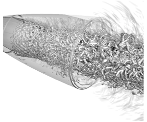
, since in these regions rotation exceeds the strain. Various patterns are visible in figures 6 and 7, including the generation of large turbulence structures in the annular supersonic shear layer, the sudden break-up of the jet core downstream and the radiation of weak Mach waves at shallow angles to the jet axis. These Mach waves are observed in the shadowgraphy images of Canchero et al. (Reference Canchero, Tinney, Murray and Ruf2016) and corroborate the findings shown here. The isosurfaces also demonstrate how the initial part of the shear layer is not dominated by azimuthally coherent rollers, which are typical of low-Reynolds-number incompressible mixing layers. In the present case, oblique modes are shown to dominate the initial part of the shear layer, leading to small-scale three-dimensional structures. This change is due to the large local convective Mach number (
$Q^{\ast }=-{\textstyle \frac{1}{2}}\unicode[STIX]{x1D608}_{ij}^{\ast }\unicode[STIX]{x1D608}_{ji}^{\ast }$
, since in these regions rotation exceeds the strain. Various patterns are visible in figures 6 and 7, including the generation of large turbulence structures in the annular supersonic shear layer, the sudden break-up of the jet core downstream and the radiation of weak Mach waves at shallow angles to the jet axis. These Mach waves are observed in the shadowgraphy images of Canchero et al. (Reference Canchero, Tinney, Murray and Ruf2016) and corroborate the findings shown here. The isosurfaces also demonstrate how the initial part of the shear layer is not dominated by azimuthally coherent rollers, which are typical of low-Reynolds-number incompressible mixing layers. In the present case, oblique modes are shown to dominate the initial part of the shear layer, leading to small-scale three-dimensional structures. This change is due to the large local convective Mach number ( $M_{c}\approx 1.03$
) at the beginning of the shear layer, in agreement with the findings of Sandham & Reynolds (Reference Sandham and Reynolds1991), who demonstrated that when
$M_{c}\approx 1.03$
) at the beginning of the shear layer, in agreement with the findings of Sandham & Reynolds (Reference Sandham and Reynolds1991), who demonstrated that when $M_{c}>1$
, oblique modes dominate the instability process in planar compressible shear layers. Similar structures were observed by Simon et al. (Reference Simon, Deck, Guillen, Sagaut and Merlen2007) in the supersonic annular shear layer past an axisymmetric trailing edge, characterized by a convective Mach number greater than one.
$M_{c}>1$
, oblique modes dominate the instability process in planar compressible shear layers. Similar structures were observed by Simon et al. (Reference Simon, Deck, Guillen, Sagaut and Merlen2007) in the supersonic annular shear layer past an axisymmetric trailing edge, characterized by a convective Mach number greater than one.

Figure 6. Visualization of the instantaneous density-gradient magnitude (numerical schlieren) along a slice through the centre of the nozzle.

Figure 7. Visualization of turbulent structures using isosurfaces of the $Q^{\ast }$
criterion.
$Q^{\ast }$
criterion.
5 Wall-pressure characteristics
5.1 Mean and standard deviation distribution
The mean wall-pressure distribution $(\,\overline{p}_{w})$
, averaged in azimuth and time, is shown in figure 8(a) alongside static wall-pressure data from the experiment. Wall pressures are shown to decrease until the incipient separation point, after which the separation shock causes an abrupt increase up to a plateau value close to ambient pressure. Data from the simulation illustrate the same findings as the experiment, except for the subtle discrepancy in the average separation shock location. This small discrepancy is attributed to two factors. The first is the unavoidable delay in the transition from RANS to LES mode (Shur et al.
Reference Shur, Spalart, Strelets and Travin2015) in the simulation, whereas the second is attributed to experimental uncertainties in the pressure-sensing system that measures NPR; these errors are estimated to be around 1 %.
$(\,\overline{p}_{w})$
, averaged in azimuth and time, is shown in figure 8(a) alongside static wall-pressure data from the experiment. Wall pressures are shown to decrease until the incipient separation point, after which the separation shock causes an abrupt increase up to a plateau value close to ambient pressure. Data from the simulation illustrate the same findings as the experiment, except for the subtle discrepancy in the average separation shock location. This small discrepancy is attributed to two factors. The first is the unavoidable delay in the transition from RANS to LES mode (Shur et al.
Reference Shur, Spalart, Strelets and Travin2015) in the simulation, whereas the second is attributed to experimental uncertainties in the pressure-sensing system that measures NPR; these errors are estimated to be around 1 %.
As for the fluctuating wall pressure, the standard deviations ( $\unicode[STIX]{x1D70E}$
) from both the simulation and experiment are shown in figure 8(b). The solid line corresponds to the DDES data and reflects the axial behaviour of
$\unicode[STIX]{x1D70E}$
) from both the simulation and experiment are shown in figure 8(b). The solid line corresponds to the DDES data and reflects the axial behaviour of $\unicode[STIX]{x1D70E}$
that is typical of a SWBLI footprint (Dolling & Or Reference Dolling and Or1985; Baars, Ruf & Tinney Reference Baars, Ruf and Tinney2015). That is, wall-pressure fluctuations are characterized by a dominant sharp peak at the separation shock location (due to shock foot oscillations that result in high and low pressures found downstream and upstream of the shock, respectively). Downstream of this oscillating shock region, pressure fluctuations relax, followed by gradual increases in fluctuation intensity with downstream distance along the nozzle wall; this is the consequence of increased intensity from Mach waves emanating from the developing separated turbulent shear layer. In order to validate the magnitude of the pressure fluctuations with the experimental data, a dashed line has been inserted in figure 8(b), whereby only the fluctuating energy up to 10 kHz is used to compute
$\unicode[STIX]{x1D70E}$
that is typical of a SWBLI footprint (Dolling & Or Reference Dolling and Or1985; Baars, Ruf & Tinney Reference Baars, Ruf and Tinney2015). That is, wall-pressure fluctuations are characterized by a dominant sharp peak at the separation shock location (due to shock foot oscillations that result in high and low pressures found downstream and upstream of the shock, respectively). Downstream of this oscillating shock region, pressure fluctuations relax, followed by gradual increases in fluctuation intensity with downstream distance along the nozzle wall; this is the consequence of increased intensity from Mach waves emanating from the developing separated turbulent shear layer. In order to validate the magnitude of the pressure fluctuations with the experimental data, a dashed line has been inserted in figure 8(b), whereby only the fluctuating energy up to 10 kHz is used to compute $\unicode[STIX]{x1D70E}$
. That is, spectra are only integrated up to 10 kHz, following Parseval’s theorem. This dashed line is in close agreement with the three experimental data points (only those pressure fluctuations below 10 kHz are considered accurate in the experiment). Since the standard deviation is an integral measure of the spectrum, it will be commented on further in § 5.2 where spectral signatures are considered.
$\unicode[STIX]{x1D70E}$
. That is, spectra are only integrated up to 10 kHz, following Parseval’s theorem. This dashed line is in close agreement with the three experimental data points (only those pressure fluctuations below 10 kHz are considered accurate in the experiment). Since the standard deviation is an integral measure of the spectrum, it will be commented on further in § 5.2 where spectral signatures are considered.

Figure 8. Distribution of $(a)$
mean wall pressure and (b) standard deviation of the wall-pressure fluctuations. Solid line, DDES; open circles, reference experimental data. For the standard deviation of the DDES, a dashed line is representative of the pressure fluctuations below 10 kHz; experimental data are resolved up to that frequency.
$(a)$
mean wall pressure and (b) standard deviation of the wall-pressure fluctuations. Solid line, DDES; open circles, reference experimental data. For the standard deviation of the DDES, a dashed line is representative of the pressure fluctuations below 10 kHz; experimental data are resolved up to that frequency.
5.2 Frequency spectra
Premultiplied wall-pressure power spectral densities, $G_{pp}(f)\cdot f/\unicode[STIX]{x1D70E}^{2}$
, are shown in figure 9 as functions of both the longitudinal coordinate
$G_{pp}(f)\cdot f/\unicode[STIX]{x1D70E}^{2}$
, are shown in figure 9 as functions of both the longitudinal coordinate $x$
and frequency
$x$
and frequency $f$
. Doing so provides a more complete picture of the spatial distribution of the energy along the nozzle wall and of the contribution of the different frequencies to the total energy of the signal. Power spectral densities are estimated using Welch’s method, i.e. subdividing the overall pressure record into 12 segments with 50 % overlap that are then individually Fourier-transformed. Frequency spectra are then obtained by averaging the periodograms of the various segments, thus minimizing the variance of the power spectral density estimator. For visualization purposes, a bandwidth moving filter, based on Konno–Ohmachi smoothing (Konno & Ohmachi Reference Konno and Ohmachi1998), has been applied, which results in a constant bandwidth on a logarithmic scale.
$f$
. Doing so provides a more complete picture of the spatial distribution of the energy along the nozzle wall and of the contribution of the different frequencies to the total energy of the signal. Power spectral densities are estimated using Welch’s method, i.e. subdividing the overall pressure record into 12 segments with 50 % overlap that are then individually Fourier-transformed. Frequency spectra are then obtained by averaging the periodograms of the various segments, thus minimizing the variance of the power spectral density estimator. For visualization purposes, a bandwidth moving filter, based on Konno–Ohmachi smoothing (Konno & Ohmachi Reference Konno and Ohmachi1998), has been applied, which results in a constant bandwidth on a logarithmic scale.

Figure 9. Contours of the premultiplied power spectral densities, $G_{pp}(f)\cdot f/\unicode[STIX]{x1D70E}^{2}$
, of the wall-pressure signals as a function of the streamwise location and frequency. Sixteen contour levels are shown in exponential scale between
$G_{pp}(f)\cdot f/\unicode[STIX]{x1D70E}^{2}$
, of the wall-pressure signals as a function of the streamwise location and frequency. Sixteen contour levels are shown in exponential scale between $10^{-4}$
and 1.
$10^{-4}$
and 1.
The spectral map in figure 9 reveals two regions with high fluctuating energy. The first region is located at the separation point ( $x/r_{t}=5.6$
), where the signature of the shock motion is visible and is characterized by a broad peak in the low-frequency range and a narrow footprint in the spatial direction. The second region is located downstream in the high-frequency range (
$x/r_{t}=5.6$
), where the signature of the shock motion is visible and is characterized by a broad peak in the low-frequency range and a narrow footprint in the spatial direction. The second region is located downstream in the high-frequency range ( $f\approx 10~\text{kHz}$
) and is associated with the developing separated shear layer, whose convected vortical structures radiate pressure disturbances that increase in intensity downstream. The overall spatial-spectral distribution of the fluctuating pressure along the expanding wall of this TIC nozzle is shown in figure 9 to be qualitatively similar to the canonical SWBLI measurements of Dupont, Haddad & Debiève (Reference Dupont, Haddad and Debiève2006), despite the significant differences in the geometrical configuration and shock topology (open separation bubble) of the present flow case.
$f\approx 10~\text{kHz}$
) and is associated with the developing separated shear layer, whose convected vortical structures radiate pressure disturbances that increase in intensity downstream. The overall spatial-spectral distribution of the fluctuating pressure along the expanding wall of this TIC nozzle is shown in figure 9 to be qualitatively similar to the canonical SWBLI measurements of Dupont, Haddad & Debiève (Reference Dupont, Haddad and Debiève2006), despite the significant differences in the geometrical configuration and shock topology (open separation bubble) of the present flow case.

Figure 10. (a–d) Premultiplied power spectral densities of the wall-pressure signals at four different $x$
locations. The solid grey line corresponds to the DDES, whereas the blue/orange lines correspond to the two experimental transducers at different azimuthal angles. Experimental data are only available for the locations of (b–d).
$x$
locations. The solid grey line corresponds to the DDES, whereas the blue/orange lines correspond to the two experimental transducers at different azimuthal angles. Experimental data are only available for the locations of (b–d).
To assist with the experimental–numerical validation of this TIC nozzle flow, premultiplied spectra of the fluctuating wall-pressure footprint are shown in figure 10(a–d) for the four representative axial stations corresponding to the vertical lines in figure 9. Note that, for the purpose of comparison, the curves are normalized by the integral of the spectra over the range of frequencies that are being resolved by the experiment (10 kHz). The first position is located immediately downstream of the separation point ( $x/r_{t}=5.6$
), whereas the other three correspond to positions where experimental data from the dynamic Kulite transducers are available (
$x/r_{t}=5.6$
), whereas the other three correspond to positions where experimental data from the dynamic Kulite transducers are available ( $x/r_{t}=12.07$
,
$x/r_{t}=12.07$
, $x/r_{t}=14.40$
and
$x/r_{t}=14.40$
and $x/r_{t}=16.73$
). At
$x/r_{t}=16.73$
). At $x/r_{t}=5.6$
in figure 10(a), the spectrum corresponding to the shock motion shows the presence of a broad, high-amplitude bump between 100 Hz and 2 kHz, with a maximum at
$x/r_{t}=5.6$
in figure 10(a), the spectrum corresponding to the shock motion shows the presence of a broad, high-amplitude bump between 100 Hz and 2 kHz, with a maximum at $f\approx 320~\text{kHz}$
and a secondary peak at intermediate frequencies around
$f\approx 320~\text{kHz}$
and a secondary peak at intermediate frequencies around $f\approx 1~\text{kHz}$
. Baars et al. (Reference Baars, Ruf and Tinney2015) ascribed the low-frequency peak to an acoustic resonance (e.g. Wong Reference Wong2005; Zaman et al.
Reference Zaman, Dahl, Bencic and Loh2002). This resonance equates to a one-quarter acoustic standing wave whose fundamental frequency can be modelled using an open-ended pipe of length
$f\approx 1~\text{kHz}$
. Baars et al. (Reference Baars, Ruf and Tinney2015) ascribed the low-frequency peak to an acoustic resonance (e.g. Wong Reference Wong2005; Zaman et al.
Reference Zaman, Dahl, Bencic and Loh2002). This resonance equates to a one-quarter acoustic standing wave whose fundamental frequency can be modelled using an open-ended pipe of length $L$
as follows:
$L$
as follows:
 $$\begin{eqnarray}f_{ac}={\displaystyle \frac{a_{\infty }(1-M_{NE}^{2})}{4L}}\approx 340~\text{Hz},\end{eqnarray}$$
where $a_{\infty }=345~\text{m}~\text{s}^{-1}$
is the ambient speed of sound and
$a_{\infty }=345~\text{m}~\text{s}^{-1}$
is the ambient speed of sound and $M_{NE}$
is the Mach number in the separated region at the nozzle exit. Here the pipe length is replaced by the distance between the incipient separation shock and the nozzle exit plane so that
$M_{NE}$
is the Mach number in the separated region at the nozzle exit. Here the pipe length is replaced by the distance between the incipient separation shock and the nozzle exit plane so that $L=0.247$
m. The value of
$L=0.247$
m. The value of $f_{ac}$
compares favourably with the 320 Hz spectral peak in figure 10(a). Moving downstream, a different picture emerges, where spectra are characterized by high frequencies (
$f_{ac}$
compares favourably with the 320 Hz spectral peak in figure 10(a). Moving downstream, a different picture emerges, where spectra are characterized by high frequencies ( $f\approx 10~\text{kHz}$
) attributed to signatures from the formation of turbulent structures in the developing shear layer. As expected, the peak frequency is shown to shift towards lower frequencies with increasing downstream position along the wall. A peak located at intermediate frequencies (
$f\approx 10~\text{kHz}$
) attributed to signatures from the formation of turbulent structures in the developing shear layer. As expected, the peak frequency is shown to shift towards lower frequencies with increasing downstream position along the wall. A peak located at intermediate frequencies ( $f\approx 1~\text{kHz}$
) is still visible in the spectra downstream of the shock foot. These peaks are imprints of the 1 kHz frequency peak observed in figure 10(a) at
$f\approx 1~\text{kHz}$
) is still visible in the spectra downstream of the shock foot. These peaks are imprints of the 1 kHz frequency peak observed in figure 10(a) at $x/r_{t}=5.6$
.
$x/r_{t}=5.6$
.
The nature of this 1 kHz tone observed in both the numerical and experimental spectra is shown to agree reasonably well up to the maximum reliable frequency threshold of the measurements. Likewise, the main features of the power spectral densities in figure 10(a–d) are also found in previous experiments involving different TIC nozzle contours (Jaunet et al. Reference Jaunet, Arbos, Lehnasch and Girard2017), or TOP nozzles operating at NPRs corresponding to FSS flow (Nguyen et al. Reference Nguyen, Deniau, Girard and Alziary de Roquefort2003; Baars et al. Reference Baars, Tinney, Ruf, Brown and McDaniels2012; Verma & Haidn Reference Verma and Haidn2014). To better characterize this 1 kHz intermediate peak, it is useful to introduce a Strouhal number, defined as (Tam, Seiner & Yu Reference Tam, Seiner and Yu1986; Canchero et al. Reference Canchero, Tinney, Murray and Ruf2016)
 $$\begin{eqnarray}St=f{\displaystyle \frac{D_{j}}{U_{j}}},\end{eqnarray}$$
where $U_{j}$
is the fully expanded jet velocity, given by
$U_{j}$
is the fully expanded jet velocity, given by
 $$\begin{eqnarray}U_{j}=\sqrt{\unicode[STIX]{x1D6FE}RT_{0}}{\displaystyle \frac{M_{j}}{\sqrt{1+{\displaystyle \frac{\unicode[STIX]{x1D6FE}-1}{2}}M_{j}^{2}}}},\end{eqnarray}$$
where $T_{0}$
is the stagnation temperature,
$T_{0}$
is the stagnation temperature, $\unicode[STIX]{x1D6FE}$
is the specific heat ratio,
$\unicode[STIX]{x1D6FE}$
is the specific heat ratio, $R$
is the air constant and
$R$
is the air constant and $M_{j}$
is the fully adapted Mach number which is a function of the NPR through the isentropic relation
$M_{j}$
is the fully adapted Mach number which is a function of the NPR through the isentropic relation
 $$\begin{eqnarray}M_{j}^{2}={\displaystyle \frac{2}{\unicode[STIX]{x1D6FE}-1}}\left[(NPR)^{(\unicode[STIX]{x1D6FE}-1)/\unicode[STIX]{x1D6FE}}-1\right].\end{eqnarray}$$
The length scale $D_{j}$
is computed as a function of
$D_{j}$
is computed as a function of $M_{j}$
, the design Mach number
$M_{j}$
, the design Mach number $M_{d}$
and the nozzle exit diameter
$M_{d}$
and the nozzle exit diameter $D$
through the mass flux conservation:
$D$
through the mass flux conservation:
 $$\begin{eqnarray}{\displaystyle \frac{D_{j}}{D}}=\left({\displaystyle \frac{1+{\displaystyle \frac{\unicode[STIX]{x1D6FE}-1}{2}}M_{j}^{2}}{1+{\displaystyle \frac{\unicode[STIX]{x1D6FE}-1}{2}}M_{d}^{2}}}\right)^{\frac{(\unicode[STIX]{x1D6FE}+1)}{(4(\unicode[STIX]{x1D6FE}-1))}}\left({\displaystyle \frac{M_{d}}{M_{j}}}\right)^{1/2}.\end{eqnarray}$$

Figure 11. Strouhal number of the intermediate peak in the frequency spectrum at the shock position as a function of the fully adapted Mach number $M_{j}$
for different geometries and NPRs.
$M_{j}$
for different geometries and NPRs.
The non-dimensional frequencies of the intermediate peak from the different experimental flow cases cited above are reported in figure 11 as a function of $M_{j}$
. A decreasing trend of
$M_{j}$
. A decreasing trend of $St$
with the fully adapted Mach number emerges, which was also identified by Jaunet et al. (Reference Jaunet, Arbos, Lehnasch and Girard2017). They proposed that this peak could be attributed to a screech-like mechanism (Raman Reference Raman1999) resulting from an aeroacoustic feedback loop involving downstream-propagating disturbances in the shear layer interacting with the shock cells to form upstream-propagating acoustic waves that excite the shear layer. According to Tam et al. (Reference Tam, Seiner and Yu1986) the screech frequency
$St$
with the fully adapted Mach number emerges, which was also identified by Jaunet et al. (Reference Jaunet, Arbos, Lehnasch and Girard2017). They proposed that this peak could be attributed to a screech-like mechanism (Raman Reference Raman1999) resulting from an aeroacoustic feedback loop involving downstream-propagating disturbances in the shear layer interacting with the shock cells to form upstream-propagating acoustic waves that excite the shear layer. According to Tam et al. (Reference Tam, Seiner and Yu1986) the screech frequency $f_{sc}$
can be evaluated as
$f_{sc}$
can be evaluated as
 $$\begin{eqnarray}St_{sc}=f_{sc}{\displaystyle \frac{D_{j}}{U_{j}}}=0.67(M_{j}^{2}-1)^{-1/2}\left[1+0.7M_{j}\left(1+{\displaystyle \frac{\unicode[STIX]{x1D6FE}-1}{2}}M_{j}^{2}\right)^{-1/2}\left({\displaystyle \frac{T_{a}}{T_{0}}}\right)^{-1/2}\right],\end{eqnarray}$$
where $T_{a}$
is the ambient temperature. The trend from the correlation in figure 11 shows that the characteristic screech frequency decreases with increasing
$T_{a}$
is the ambient temperature. The trend from the correlation in figure 11 shows that the characteristic screech frequency decreases with increasing $M_{j}$
(or equivalently with increasing NPR), mainly due to the increase in shock cell spacing. Despite a certain level of dispersion, the proximity of the experimental data and of the DDES prediction to the theoretical correlation suggests that the intermediate peak could be attributed to a screech-like phenomenon associated with the shock cell structure present within the nozzle. Nevertheless, it must be pointed out that the shock cell spacing used in Tam’s model, which is derived from a parallel flow assumption (Pack Reference Pack1950), is
$M_{j}$
(or equivalently with increasing NPR), mainly due to the increase in shock cell spacing. Despite a certain level of dispersion, the proximity of the experimental data and of the DDES prediction to the theoretical correlation suggests that the intermediate peak could be attributed to a screech-like phenomenon associated with the shock cell structure present within the nozzle. Nevertheless, it must be pointed out that the shock cell spacing used in Tam’s model, which is derived from a parallel flow assumption (Pack Reference Pack1950), is $L/D_{j}=2.81$
. This model is usually adopted to study under- and overexpanded jets, without flow separation. Instead, the configuration investigated here manifests a large recirculation region inside the nozzle, with a Mach reflection characterized by the angle of the oblique shock, which is very different from
$L/D_{j}=2.81$
. This model is usually adopted to study under- and overexpanded jets, without flow separation. Instead, the configuration investigated here manifests a large recirculation region inside the nozzle, with a Mach reflection characterized by the angle of the oblique shock, which is very different from $\unicode[STIX]{x03C0}/2$
(with respect to the nozzle longitudinal axis). As a consequence we have two characteristic distances
$\unicode[STIX]{x03C0}/2$
(with respect to the nozzle longitudinal axis). As a consequence we have two characteristic distances $L_{s,1}=2.38D_{j}$
and
$L_{s,1}=2.38D_{j}$
and $L_{s,2}=3.35D_{j}$
, corresponding to the distances from the Mach disk and separation shock foot to the second normal shock, respectively. A feedback-loop model adapted to accommodate the unique flow and shock pattern produced by this TIC nozzle is proposed and discussed in § 7. There it will be shown that the larger length scales of the present configuration are partially compensated by characteristic velocities that differ from what was applied in Tam’s model, thereby offering good agreement with the corollary of (5.6) for the present flow case.
$L_{s,2}=3.35D_{j}$
, corresponding to the distances from the Mach disk and separation shock foot to the second normal shock, respectively. A feedback-loop model adapted to accommodate the unique flow and shock pattern produced by this TIC nozzle is proposed and discussed in § 7. There it will be shown that the larger length scales of the present configuration are partially compensated by characteristic velocities that differ from what was applied in Tam’s model, thereby offering good agreement with the corollary of (5.6) for the present flow case.
5.3 Space–time correlations and convection velocity
Additional insights into the propagation of pressure disturbances, in terms of direction and velocity, can be gained by inspection of the space–time correlation coefficient, defined as
 $$\begin{eqnarray}C_{pp}(x,\unicode[STIX]{x0394}x,\unicode[STIX]{x0394}\unicode[STIX]{x1D703},\unicode[STIX]{x0394}\unicode[STIX]{x1D70F})={\displaystyle \frac{R_{pp}(x,\unicode[STIX]{x0394}x,\unicode[STIX]{x0394}\unicode[STIX]{x1D703},\unicode[STIX]{x0394}\unicode[STIX]{x1D70F})}{\left[R_{pp}(x,0,0,0)\right]^{1/2}\,\left[R_{pp}(x,\unicode[STIX]{x0394}x,0,0)\right]^{1/2}}},\end{eqnarray}$$
where
 $$\begin{eqnarray}R_{pp}(x,\unicode[STIX]{x0394}x,\unicode[STIX]{x0394}\unicode[STIX]{x1D703},\unicode[STIX]{x0394}\unicode[STIX]{x1D70F})=\langle p_{w}^{^{\prime }}(x,\unicode[STIX]{x1D703},t)\,p_{w}^{^{\prime }}(x+\unicode[STIX]{x0394}x,\unicode[STIX]{x1D703}+\unicode[STIX]{x0394}\unicode[STIX]{x1D703},t+\unicode[STIX]{x0394}\unicode[STIX]{x1D70F})\rangle\end{eqnarray}$$
is the space–time correlation function, $\unicode[STIX]{x0394}x$
and
$\unicode[STIX]{x0394}x$
and $\unicode[STIX]{x0394}\unicode[STIX]{x1D703}$
are the spatial separations in the streamwise and azimuthal directions,
$\unicode[STIX]{x0394}\unicode[STIX]{x1D703}$
are the spatial separations in the streamwise and azimuthal directions, $\unicode[STIX]{x0394}\unicode[STIX]{x1D70F}$
is the time delay and
$\unicode[STIX]{x0394}\unicode[STIX]{x1D70F}$
is the time delay and $\langle ~\rangle$
denotes averaging with respect to the azimuthal direction (exploiting homogeneity) and time. Figure 12(a,b) reports contours of this space–time correlation coefficient
$\langle ~\rangle$
denotes averaging with respect to the azimuthal direction (exploiting homogeneity) and time. Figure 12(a,b) reports contours of this space–time correlation coefficient $C_{pp}(x,\unicode[STIX]{x0394}x,0,\unicode[STIX]{x0394}\unicode[STIX]{x1D70F})$
taken at two stations along the nozzle wall at
$C_{pp}(x,\unicode[STIX]{x0394}x,0,\unicode[STIX]{x0394}\unicode[STIX]{x1D70F})$
taken at two stations along the nozzle wall at $x/r_{t}=8$
and
$x/r_{t}=8$
and $x/r_{t}=14$
. At both positions, the shapes of the contours reflect the convective nature of the pressure field. Albeit, the pressure signal is mainly characterized by a coherent downstream propagation of pressure-carrying eddies at the downstream station (
$x/r_{t}=14$
. At both positions, the shapes of the contours reflect the convective nature of the pressure field. Albeit, the pressure signal is mainly characterized by a coherent downstream propagation of pressure-carrying eddies at the downstream station ( $x/r_{t}=14$
), while at the upstream location (
$x/r_{t}=14$
), while at the upstream location ( $x/r_{t}=8$
) the presence of upstream-propagating disturbances is well visible.
$x/r_{t}=8$
) the presence of upstream-propagating disturbances is well visible.

Figure 12. (a,b) Space–time contours of the pressure correlation coefficient $C_{pp}(\unicode[STIX]{x0394}x,0,\unicode[STIX]{x0394}\unicode[STIX]{x1D70F})$
using 11 contour levels in the range
$C_{pp}(\unicode[STIX]{x0394}x,0,\unicode[STIX]{x0394}\unicode[STIX]{x1D70F})$
using 11 contour levels in the range $-0.1<C_{pp}<0.9$
. (c,d) Local convection velocity of wall-pressure fluctuations as a function of the time separation
$-0.1<C_{pp}<0.9$
. (c,d) Local convection velocity of wall-pressure fluctuations as a function of the time separation $\unicode[STIX]{x0394}\unicode[STIX]{x1D70F}$
.
$\unicode[STIX]{x0394}\unicode[STIX]{x1D70F}$
.
From the maps of the space–time correlation coefficient it is possible to evaluate the convection velocities of the pressure-carrying eddies. Following Bernardini & Pirozzoli (Reference Bernardini and Pirozzoli2011), the convection speed corresponding to a given time delay $\unicode[STIX]{x0394}\unicode[STIX]{x1D70F}$
is defined as the ratio
$\unicode[STIX]{x0394}\unicode[STIX]{x1D70F}$
is defined as the ratio $\unicode[STIX]{x0394}x/\unicode[STIX]{x0394}\unicode[STIX]{x1D70F}$
taken at the spatial separation value
$\unicode[STIX]{x0394}x/\unicode[STIX]{x0394}\unicode[STIX]{x1D70F}$
taken at the spatial separation value $\unicode[STIX]{x0394}x$
where a local maximum of
$\unicode[STIX]{x0394}x$
where a local maximum of $C_{pp}$
is attained. The resulting convection speeds are displayed in figure 12(c,d), as a function of the time separation
$C_{pp}$
is attained. The resulting convection speeds are displayed in figure 12(c,d), as a function of the time separation $\unicode[STIX]{x0394}\unicode[STIX]{x1D70F}$
. We see that the convection speeds range from
$\unicode[STIX]{x0394}\unicode[STIX]{x1D70F}$
. We see that the convection speeds range from $0.6u_{j}$
to
$0.6u_{j}$
to $0.7u_{j}$
, in agreement with the value quoted by Tam et al. (Reference Tam, Seiner and Yu1986). There is also an absence of upstream-propagating disturbances in the space–time map of figure 12(b) which reinforces the notion that the unsteady pressure field at
$0.7u_{j}$
, in agreement with the value quoted by Tam et al. (Reference Tam, Seiner and Yu1986). There is also an absence of upstream-propagating disturbances in the space–time map of figure 12(b) which reinforces the notion that the unsteady pressure field at $x/r_{t}=14$
is dominated by signatures from energetic, high-frequency, downstream-travelling vortices in the separated shear layer.
$x/r_{t}=14$
is dominated by signatures from energetic, high-frequency, downstream-travelling vortices in the separated shear layer.
For a more rigorous inspection of the propagation speeds of these disturbances, a frequency-dependent convection velocity $u_{c}(f)$
is computed according to the formulation proposed by Renard & Deck (Reference Renard and Deck2015):
$u_{c}(f)$
is computed according to the formulation proposed by Renard & Deck (Reference Renard and Deck2015):
 $$\begin{eqnarray}u_{c}(f)={\displaystyle \frac{-2\unicode[STIX]{x03C0}f\,G_{pp}(f)}{\text{Im}\left(G_{pp^{\prime }}(f)\right)}},\end{eqnarray}$$
where $G_{pp^{\prime }}$
is the cross-spectrum between the pressure signal and its streamwise derivative (
$G_{pp^{\prime }}$
is the cross-spectrum between the pressure signal and its streamwise derivative ( $p^{\prime }=\unicode[STIX]{x2202}p/\unicode[STIX]{x2202}x$
). In the case of a simple monochromatic wave, equation (5.9) can be interpreted as the phase velocity, whereas in the general case its interpretation relies on the least-squares minimization of the convection equation residual, consistent with del Álamo & Jiménez (Reference del Álamo and Jiménez2009). This spectral approach is a generalization of previous methods based on the phase between signals taken at two streamwise points (Romano Reference Romano1995). The upside to this approach is that it offers a direct assessment of scale dependence without having to band-pass filter the signals, thus preventing aliasing and/or phase alterations. Moreover, the method inherently includes the definition of a global convection velocity:
$p^{\prime }=\unicode[STIX]{x2202}p/\unicode[STIX]{x2202}x$
). In the case of a simple monochromatic wave, equation (5.9) can be interpreted as the phase velocity, whereas in the general case its interpretation relies on the least-squares minimization of the convection equation residual, consistent with del Álamo & Jiménez (Reference del Álamo and Jiménez2009). This spectral approach is a generalization of previous methods based on the phase between signals taken at two streamwise points (Romano Reference Romano1995). The upside to this approach is that it offers a direct assessment of scale dependence without having to band-pass filter the signals, thus preventing aliasing and/or phase alterations. Moreover, the method inherently includes the definition of a global convection velocity:
 $$\begin{eqnarray}C_{u}=-{\displaystyle \frac{\int _{0}^{\infty }\left(2\unicode[STIX]{x03C0}f\right)^{2}\,G_{pp}(f)\,\text{d}f}{\int _{0}^{\infty }2\unicode[STIX]{x03C0}f\,\text{Im}(G_{pp^{\prime }}(f))\,\text{d}f}},\end{eqnarray}$$
which can be shown to coincide with derived methods based on space–time correlations (Renard & Deck Reference Renard and Deck2015). The distribution of $u_{c}$
as a function of frequency
$u_{c}$
as a function of frequency $f$
is reported in figure 13 for the probe at
$f$
is reported in figure 13 for the probe at $x/r_{t}=14$
. The illustration clearly reveals how all frequencies leading up to the intermediate frequency of 1 kHz (
$x/r_{t}=14$
. The illustration clearly reveals how all frequencies leading up to the intermediate frequency of 1 kHz ( $St=0.12$
) correspond to upstream-travelling waves. At this intermediate frequency,
$St=0.12$
) correspond to upstream-travelling waves. At this intermediate frequency, $u_{c}(f)$
diverges before switching to positive values. Such divergence could be explained by the formation of a standing wave arising from the interference of two travelling waves moving in the opposite direction that produce a zero phase value in the denominator of equation (5.9). This behaviour reinforces the postulation that the intermediate-frequency peak in the spectra is related to a screech-like process, which is classically associated with the formation of a standing wave generated by downstream-propagating hydrodynamic and upstream-propagating acoustic fluctuations (Tam Reference Tam1995). Consistent with the results of the broadband analysis, the convection velocity associated with the high-frequency range in figure 13 is approximately equal to
$u_{c}(f)$
diverges before switching to positive values. Such divergence could be explained by the formation of a standing wave arising from the interference of two travelling waves moving in the opposite direction that produce a zero phase value in the denominator of equation (5.9). This behaviour reinforces the postulation that the intermediate-frequency peak in the spectra is related to a screech-like process, which is classically associated with the formation of a standing wave generated by downstream-propagating hydrodynamic and upstream-propagating acoustic fluctuations (Tam Reference Tam1995). Consistent with the results of the broadband analysis, the convection velocity associated with the high-frequency range in figure 13 is approximately equal to $0.7u_{j}$
.
$0.7u_{j}$
.

Figure 13. Frequency-dependent convection velocity at $x/r_{t}=14$
. The red horizontal dashed line denotes the value
$x/r_{t}=14$
. The red horizontal dashed line denotes the value $0.7u_{j}$
.
$0.7u_{j}$
.

Figure 14. Contours of the premultiplied azimuthal wavenumber–frequency spectra $\unicode[STIX]{x1D719}_{pp}(f)\cdot f/\unicode[STIX]{x1D70E}^{2}$
at two different axial locations. Twenty contour levels are shown in exponential scale between 0.005 and 5.
$\unicode[STIX]{x1D719}_{pp}(f)\cdot f/\unicode[STIX]{x1D70E}^{2}$
at two different axial locations. Twenty contour levels are shown in exponential scale between 0.005 and 5.
5.4 Azimuthal decomposition of the pressure field
In order to gain insights into the origins of the aerodynamic loads acting on the TIC nozzle wall, and to characterize the wavenumbers that make up the unsteady wall-pressure footprint, then it is natural to carry out a Fourier-azimuthal decomposition of the fluctuating wall-pressure signatures. To that end, we consider the azimuthal wavenumber–frequency spectrum, defined as
 $$\begin{eqnarray}\unicode[STIX]{x1D719}_{pp}(x,m,f)=\int _{-\infty }^{\infty }\int _{0}^{2\unicode[STIX]{x03C0}}R_{pp}(x,0,\unicode[STIX]{x0394}\unicode[STIX]{x1D703},\unicode[STIX]{x0394}\unicode[STIX]{x1D70F})\,\text{e}^{-\text{i}(m\unicode[STIX]{x0394}\unicode[STIX]{x1D703}+f\unicode[STIX]{x0394}\unicode[STIX]{x1D70F})}\text{d}(\unicode[STIX]{x0394}\unicode[STIX]{x1D703})\,\text{d}(\unicode[STIX]{x0394}\unicode[STIX]{x1D70F}),\end{eqnarray}$$
where $m$
is the Fourier-azimuthal wavenumber (or mode number). We remind ourselves that, according to symmetry, only the non-axisymmetric mode
$m$
is the Fourier-azimuthal wavenumber (or mode number). We remind ourselves that, according to symmetry, only the non-axisymmetric mode $m=1$
will contribute to off-axis aerodynamic side loads.
$m=1$
will contribute to off-axis aerodynamic side loads.
The azimuthal wavenumber–frequency spectrum $\unicode[STIX]{x1D719}_{pp}$
is reported in figure 14 for two representative stations, corresponding to the location immediately downstream of the separation shock at
$\unicode[STIX]{x1D719}_{pp}$
is reported in figure 14 for two representative stations, corresponding to the location immediately downstream of the separation shock at $x/r_{t}=5.6$
(figure 14
a) and in the upstream-travelling entrained flow region at
$x/r_{t}=5.6$
(figure 14
a) and in the upstream-travelling entrained flow region at $x/r_{t}=14.4$
(figure 14
b). One can see that the preponderance of energy is confined to the first few Fourier-azimuthal modes, and is complementary to the experimental analysis of Baars & Tinney (Reference Baars and Tinney2013). To better quantify the spectral make-up of the dominant azimuthal modes along the nozzle wall, slices through the wavenumber–frequency maps for the first two discrete azimuthal modes (
$x/r_{t}=14.4$
(figure 14
b). One can see that the preponderance of energy is confined to the first few Fourier-azimuthal modes, and is complementary to the experimental analysis of Baars & Tinney (Reference Baars and Tinney2013). To better quantify the spectral make-up of the dominant azimuthal modes along the nozzle wall, slices through the wavenumber–frequency maps for the first two discrete azimuthal modes ( $m=0$
and
$m=0$
and $m=1$
) are reported in figure 15. This figure reveals how the shock motion at
$m=1$
) are reported in figure 15. This figure reveals how the shock motion at $x/r_{t}=5.6$
in figure 15(a) has a clear organization in the azimuthal direction with a dominant peak at
$x/r_{t}=5.6$
in figure 15(a) has a clear organization in the azimuthal direction with a dominant peak at $f\approx 320$
Hz (
$f\approx 320$
Hz ( $St=0.038$
) exclusively associated with the axisymmetric (breathing) mode
$St=0.038$
) exclusively associated with the axisymmetric (breathing) mode $m=0$
. The secondary peak at
$m=0$
. The secondary peak at $f\approx 1~\text{kHz}$
(
$f\approx 1~\text{kHz}$
( $St=0.12$
) is then shown in figure 15(b) to be linked to the first (
$St=0.12$
) is then shown in figure 15(b) to be linked to the first ( $m=1$
) Fourier mode. The emerging picture is that of a separation shock characterized by a low-frequency piston-like motion coupled with excitation from the off-axis mode at intermediate frequencies. Moving downstream to
$m=1$
) Fourier mode. The emerging picture is that of a separation shock characterized by a low-frequency piston-like motion coupled with excitation from the off-axis mode at intermediate frequencies. Moving downstream to $x/r_{t}=14.4$
, the contribution of the breathing mode at low frequencies becomes less significant, whereas the peak located at
$x/r_{t}=14.4$
, the contribution of the breathing mode at low frequencies becomes less significant, whereas the peak located at $f\approx 1~\text{kHz}$
(
$f\approx 1~\text{kHz}$
( $St\approx 0.12$
) for
$St\approx 0.12$
) for $m=1$
still persists, suggesting the presence of helical/flapping modes in the separated shear layer, also highlighted by the dominant
$m=1$
still persists, suggesting the presence of helical/flapping modes in the separated shear layer, also highlighted by the dominant $m=1$
dynamics of the high-frequency fluctuations. This observation provides additional support to the screech-like nature of the intermediate peak frequency, since previous experimental and theoretical analyses have shown that at high fully adapted Mach numbers (
$m=1$
dynamics of the high-frequency fluctuations. This observation provides additional support to the screech-like nature of the intermediate peak frequency, since previous experimental and theoretical analyses have shown that at high fully adapted Mach numbers ( $M_{j}>1.3$
) the helical instability wave mode has larger total growth at frequencies close to the screech tone (Tam Reference Tam1995; Seiner, Manning & Ponton Reference Seiner, Manning and Ponton1987). As previously observed in the spectra at this location (
$M_{j}>1.3$
) the helical instability wave mode has larger total growth at frequencies close to the screech tone (Tam Reference Tam1995; Seiner, Manning & Ponton Reference Seiner, Manning and Ponton1987). As previously observed in the spectra at this location ( $x/r_{t}=14.4$
) in figure 10(c), most of the energy is a manifestation of high-frequency activity spread over a broad range of azimuthal modes thereby reflecting the turbulent character of the wall-pressure fluctuations in this subsonic recirculation region.
$x/r_{t}=14.4$
) in figure 10(c), most of the energy is a manifestation of high-frequency activity spread over a broad range of azimuthal modes thereby reflecting the turbulent character of the wall-pressure fluctuations in this subsonic recirculation region.

Figure 15. Premultiplied spectra of the (a) zeroth and (b) first Fourier azimuthal mode at two axial locations.

Figure 16. Contour of $\unicode[STIX]{x2202}\unicode[STIX]{x1D70C}/\unicode[STIX]{x2202}x$
from the TIC nozzle flow simulation showing pressure waves radiating from vortical structures in the separated shear layers.
$\unicode[STIX]{x2202}\unicode[STIX]{x1D70C}/\unicode[STIX]{x2202}x$
from the TIC nozzle flow simulation showing pressure waves radiating from vortical structures in the separated shear layers.
6 Annular supersonic shear layer and Mach disk region
Instantaneous snapshots of the simulated flow are now scrutinized to assess the existence and evolution of coherent vortices along the detached shear layer. Beginning with figure 16, the streamwise derivative of the density field, $\unicode[STIX]{x2202}\unicode[STIX]{x1D70C}/\unicode[STIX]{x2202}x$
, is illustrated for the upstream regions of the separated shear layer where black and white contrasts correspond to compressions (or shocks) and expansions of the gas, respectively. Apparent from this illustration is the formation of coherent vortices that interact with both the separation and reflected shocks. These vortices form at the beginning of the shear layer and are highlighted by the presence of pressure waves extending towards the core of the nozzle where the flow is supersonic. The latter of these shocks is reflected as an expansion fan as it interacts with the upper boundary of the annular shear layer. A close inspection of the evolution of these shear-layer structures is then tracked in figure 17 using a sequence of snapshots of the streamwise component of the density gradient. The eddies comprise elliptical-shaped patterns that remain, for the most part, unchanged and without merging with neighbouring structures, until they interact with the reflected shock. These observations are complementary to those reported by Simon et al. (Reference Simon, Deck, Guillen, Sagaut and Merlen2007) in their analysis of vortex dynamics in a compressible shear layer past an axisymmetric trailing edge. Simon et al. (Reference Simon, Deck, Guillen, Sagaut and Merlen2007) reported instances of merging between vortices, but without the well-known rotational pairing that contributes to the growth rate of subsonic shear layers.
$\unicode[STIX]{x2202}\unicode[STIX]{x1D70C}/\unicode[STIX]{x2202}x$
, is illustrated for the upstream regions of the separated shear layer where black and white contrasts correspond to compressions (or shocks) and expansions of the gas, respectively. Apparent from this illustration is the formation of coherent vortices that interact with both the separation and reflected shocks. These vortices form at the beginning of the shear layer and are highlighted by the presence of pressure waves extending towards the core of the nozzle where the flow is supersonic. The latter of these shocks is reflected as an expansion fan as it interacts with the upper boundary of the annular shear layer. A close inspection of the evolution of these shear-layer structures is then tracked in figure 17 using a sequence of snapshots of the streamwise component of the density gradient. The eddies comprise elliptical-shaped patterns that remain, for the most part, unchanged and without merging with neighbouring structures, until they interact with the reflected shock. These observations are complementary to those reported by Simon et al. (Reference Simon, Deck, Guillen, Sagaut and Merlen2007) in their analysis of vortex dynamics in a compressible shear layer past an axisymmetric trailing edge. Simon et al. (Reference Simon, Deck, Guillen, Sagaut and Merlen2007) reported instances of merging between vortices, but without the well-known rotational pairing that contributes to the growth rate of subsonic shear layers.

Figure 17. Convection of coherent structures in the separated shear layer, shown by means of contours of $\unicode[STIX]{x2202}\unicode[STIX]{x1D70C}/\unicode[STIX]{x2202}x$
. Instantaneous snapshots
$\unicode[STIX]{x2202}\unicode[STIX]{x1D70C}/\unicode[STIX]{x2202}x$
. Instantaneous snapshots $\unicode[STIX]{x0394}t=1.3\times 10^{-5}$
s apart from left to right.
$\unicode[STIX]{x0394}t=1.3\times 10^{-5}$
s apart from left to right.
A spectral characterization of the static pressure within the shear layer is now examined using six probe locations, denoted by $P_{1}$
–
$P_{1}$
– $P_{6}$
in figure 18(a). The power spectral densities of the six time series are shown in figure 18(b,c). The first four probes are located before the interaction of the reflected shock with the shear layer, whereas the last two probes are placed downstream of this interaction. The signal from probe
$P_{6}$
in figure 18(a). The power spectral densities of the six time series are shown in figure 18(b,c). The first four probes are located before the interaction of the reflected shock with the shear layer, whereas the last two probes are placed downstream of this interaction. The signal from probe $P_{1}$
is characterized by a small peak centred around 320 Hz (
$P_{1}$
is characterized by a small peak centred around 320 Hz ( $St=0.038$
), which is clearly linked to the shock movement. The second high-frequency and high-energy broad peak is centred around 20 kHz (
$St=0.038$
), which is clearly linked to the shock movement. The second high-frequency and high-energy broad peak is centred around 20 kHz ( $S_{t}=2.41$
) and corresponds to the signature of the dominant shear-layer instability, a feature also visible in the spectra at the downstream probes. From the numerical schlieren images (e.g. figure 17) it is also evident that acoustic disturbances from the region spanned by
$S_{t}=2.41$
) and corresponds to the signature of the dominant shear-layer instability, a feature also visible in the spectra at the downstream probes. From the numerical schlieren images (e.g. figure 17) it is also evident that acoustic disturbances from the region spanned by $P_{1}$
–
$P_{1}$
– $P_{3}$
propagate towards the nozzle wall. This is coupled to the spectra imprint on the wall around 10–20 kHz and starting from
$P_{3}$
propagate towards the nozzle wall. This is coupled to the spectra imprint on the wall around 10–20 kHz and starting from $x_{r_{t}}\approx 12$
, as was described in the discussion of figure 9. Moving to
$x_{r_{t}}\approx 12$
, as was described in the discussion of figure 9. Moving to $P_{5}$
and
$P_{5}$
and $P_{6}$
in figure 18(b,c), it is observed that the high-frequency component spreads to lower frequencies while the spectral peaks broaden due to the growth of the turbulent structures in the developing shear layer. The contribution of the 320 Hz low-frequency peak reduces moving in the downstream direction and the spectra appear relatively flat in the low-/intermediate-frequency range. This behaviour is consistent with a screech-like scenario where the mixing layer may represent the first path for the downstream propagation of disturbances.
$P_{6}$
in figure 18(b,c), it is observed that the high-frequency component spreads to lower frequencies while the spectral peaks broaden due to the growth of the turbulent structures in the developing shear layer. The contribution of the 320 Hz low-frequency peak reduces moving in the downstream direction and the spectra appear relatively flat in the low-/intermediate-frequency range. This behaviour is consistent with a screech-like scenario where the mixing layer may represent the first path for the downstream propagation of disturbances.

Figure 18. (a) Positions of the numerical pressure probes. (b,c) Pressure spectra along the separated shear layer (from $P_{1}$
to
$P_{1}$
to $P_{6}$
).
$P_{6}$
).
Downstream of the Mach disk, the flow is characterized by intense vortex shedding activity and consequent production of vorticity, as highlighted by the sequence of snapshots of $\unicode[STIX]{x2202}\unicode[STIX]{x1D70C}/\unicode[STIX]{x2202}x$
reported in figure 19. In figure 19(a), the Mach disk is bent upstream while two counter-rotating vortices are emitted. According to Nasuti & Onofri (Reference Nasuti and Onofri2009), the bending of the Mach disk is caused by two factors. Foremost, the Mach number field upstream of the shock region is not uniform, especially in the radial direction, as is clearly shown in figure 5. Therefore, in order for the flow to adapt to the new static pressure in the subsonic flow after the Mach disk (which is nearly uniform in a time- and space-average sense) the shock has to adjust its curvature radially in order to change intensity. Secondly, the flow unsteadiness causes a continuous variation in the static pressure behind the shock, which causes the Mach disk to oscillate and its curvature to vary. The change in shock intensity along the radial direction causes an entropy gradient downstream and, as described by the Crocco theorem (Crocco Reference Crocco1937), vorticity to be produced. These vortical structures then convect downstream and impinge on both the annular supersonic shear layer and the second shock cell, in a non-symmetric way. In the last snapshot in figure 19(d),
$\unicode[STIX]{x2202}\unicode[STIX]{x1D70C}/\unicode[STIX]{x2202}x$
reported in figure 19. In figure 19(a), the Mach disk is bent upstream while two counter-rotating vortices are emitted. According to Nasuti & Onofri (Reference Nasuti and Onofri2009), the bending of the Mach disk is caused by two factors. Foremost, the Mach number field upstream of the shock region is not uniform, especially in the radial direction, as is clearly shown in figure 5. Therefore, in order for the flow to adapt to the new static pressure in the subsonic flow after the Mach disk (which is nearly uniform in a time- and space-average sense) the shock has to adjust its curvature radially in order to change intensity. Secondly, the flow unsteadiness causes a continuous variation in the static pressure behind the shock, which causes the Mach disk to oscillate and its curvature to vary. The change in shock intensity along the radial direction causes an entropy gradient downstream and, as described by the Crocco theorem (Crocco Reference Crocco1937), vorticity to be produced. These vortical structures then convect downstream and impinge on both the annular supersonic shear layer and the second shock cell, in a non-symmetric way. In the last snapshot in figure 19(d), $t=3.46\times 10^{-2}$
s, two new counter-rotating vortices have formed, but are now located below the centreline of the nozzle, thus indicating the non-symmetric behaviour of this shedding phenomenon. An inspection of the flow field along the simulation time also reveals that this activity is not continuous but rather intermittent, as clearly highlighted by the accompanying movie available online at https://doi.org/10.1017/jfm.2020.280.
$t=3.46\times 10^{-2}$
s, two new counter-rotating vortices have formed, but are now located below the centreline of the nozzle, thus indicating the non-symmetric behaviour of this shedding phenomenon. An inspection of the flow field along the simulation time also reveals that this activity is not continuous but rather intermittent, as clearly highlighted by the accompanying movie available online at https://doi.org/10.1017/jfm.2020.280.

Figure 19. Contours of $\unicode[STIX]{x2202}\unicode[STIX]{x1D70C}/\unicode[STIX]{x2202}x$
showing convection of coherent structures downstream of the Mach disk. Instantaneous snapshots at (a)
$\unicode[STIX]{x2202}\unicode[STIX]{x1D70C}/\unicode[STIX]{x2202}x$
showing convection of coherent structures downstream of the Mach disk. Instantaneous snapshots at (a) $t=3.36\times 10^{-2}~\text{s}$
, (b)
$t=3.36\times 10^{-2}~\text{s}$
, (b) $t=3.39\times 10^{-2}~\text{s}$
, (c)
$t=3.39\times 10^{-2}~\text{s}$
, (c) $t=3.43\times 10^{-2}~\text{s}$
and
$t=3.43\times 10^{-2}~\text{s}$
and $(d)$
$(d)$ $t=3.46\times 10^{-2}~\text{s}$
.
$t=3.46\times 10^{-2}~\text{s}$
.
To further investigate the dynamics of the simulated flow, several additional probes have been placed downstream of the Mach disk (near the nozzle axis) and in the inner shear layer that originates from the triple point of the separation shock reflection, as shown by figure 18(a). Figure 20(a) shows the premultiplied spectra of the static pressure downstream of the Mach disk. The signal from the first probe ( $D_{1}$
) is characterized by a very broad bump, with the highest peak residing at 905 Hz (
$D_{1}$
) is characterized by a very broad bump, with the highest peak residing at 905 Hz ( $St=0.11$
). The energy associated with this peak originates from unsteady motions of the Mach disk, whose energy decreases rapidly downstream, as shown by the spectra at
$St=0.11$
). The energy associated with this peak originates from unsteady motions of the Mach disk, whose energy decreases rapidly downstream, as shown by the spectra at $D_{2}$
and
$D_{2}$
and $D_{3}$
. The internal vortices shed by the Mach disk radiate pressure waves as they convect, stretch and break apart into smaller scales, which explains the broad shape in the spectra. Concerning the probe at
$D_{3}$
. The internal vortices shed by the Mach disk radiate pressure waves as they convect, stretch and break apart into smaller scales, which explains the broad shape in the spectra. Concerning the probe at $TP_{1}$
, located in the initial part of the inner shear layer (see figure 18
a), the spectrum reported in figure 20(b) reveals the presence of a dominant peak in the intermediate range (
$TP_{1}$
, located in the initial part of the inner shear layer (see figure 18
a), the spectrum reported in figure 20(b) reveals the presence of a dominant peak in the intermediate range ( $St=0.11$
), with significant energy at the resonant frequency of 1 kHz, associated with the first Fourier-azimuthal mode (see the discussion in § 5). Moving downstream (probe
$St=0.11$
), with significant energy at the resonant frequency of 1 kHz, associated with the first Fourier-azimuthal mode (see the discussion in § 5). Moving downstream (probe $TP_{2}$
), the relative importance of the intermediate peak reduces due to the development of the turbulent shear layer, highlighted by a broad peak around 7 kHz (
$TP_{2}$
), the relative importance of the intermediate peak reduces due to the development of the turbulent shear layer, highlighted by a broad peak around 7 kHz ( $St=0.843$
).
$St=0.843$
).

Figure 20. Premultiplied frequency spectra of the pressure signal downstream of the Mach disk (a) from $D_{1}$
to
$D_{1}$
to $D_{3}$
and (b) along the internal shear layer past the triple point (
$D_{3}$
and (b) along the internal shear layer past the triple point ( $TP_{1}$
and
$TP_{1}$
and $TP_{2}$
).
$TP_{2}$
).
To characterize the spatial development of the turbulent structures in the core and inner shear-layer regions of this TIC nozzle flow, a global value of the convection velocity has been computed according to (5.10), using the velocity signals taken along a series of probes shown in figure 21(a), ranging from the Mach disk up to the second shock. The distribution of $C_{u}$
is reported in figure 21(b) as a function of the streamwise coordinate of the probes. In this region, the flow is characterized by strong accelerations and so it is not surprising to see variations in the convection velocity ranging from a minimum value of
$C_{u}$
is reported in figure 21(b) as a function of the streamwise coordinate of the probes. In this region, the flow is characterized by strong accelerations and so it is not surprising to see variations in the convection velocity ranging from a minimum value of $C_{u}=0.3u_{j}$
upstream at
$C_{u}=0.3u_{j}$
upstream at $x/r_{t}=10.2$
to a maximum value of
$x/r_{t}=10.2$
to a maximum value of $C_{u}\approx u_{j}$
downstream. If the total time
$C_{u}\approx u_{j}$
downstream. If the total time $T_{s,1}$
needed by a turbulent structure to cover the distance between the Mach disk and the second normal shock (
$T_{s,1}$
needed by a turbulent structure to cover the distance between the Mach disk and the second normal shock ( $L_{s,1}$
) is computed by integrating the distribution of
$L_{s,1}$
) is computed by integrating the distribution of $C_{u}(x)$
along the streamwise direction, then an average value of the convection velocity for the downstream-propagating disturbances is found to be
$C_{u}(x)$
along the streamwise direction, then an average value of the convection velocity for the downstream-propagating disturbances is found to be $\overline{C}_{u}=L_{s,1}/T_{s,1}=0.72\,u_{j}$
.
$\overline{C}_{u}=L_{s,1}/T_{s,1}=0.72\,u_{j}$
.
7 Aeroacoustic feedback loop mechanism
It has been shown that the wall-pressure signatures are characterized by the presence of a peak at an intermediate frequency around $f\approx 1~\text{kHz}$
(
$f\approx 1~\text{kHz}$
( $St\approx 0.12$
), which is visible both at the shock location and in the downstream region of the nozzle wall where the developing shear layer resides. It has also been shown how this intermediate frequency agrees with the correlation proposed by Tam et al. (Reference Tam, Seiner and Yu1986) and is associated with the first Fourier-azimuthal mode (
$St\approx 0.12$
), which is visible both at the shock location and in the downstream region of the nozzle wall where the developing shear layer resides. It has also been shown how this intermediate frequency agrees with the correlation proposed by Tam et al. (Reference Tam, Seiner and Yu1986) and is associated with the first Fourier-azimuthal mode ( $m=1$
), which happens to be the only mode contributing to the generation of off-axis side loads. Similar results were also observed in the experiments of Jaunet et al. (Reference Jaunet, Arbos, Lehnasch and Girard2017). In that, screech tones were not observed in the external ambient field and the existence was postulated of a screech-like mechanism inside the nozzle that was sustained by the presence of the internal subsonic flow region downstream of the Mach disk as the pathway for upstream-propagating waves. The numerical findings from the current DDES model support the existence of an internal feedback loop.
$m=1$
), which happens to be the only mode contributing to the generation of off-axis side loads. Similar results were also observed in the experiments of Jaunet et al. (Reference Jaunet, Arbos, Lehnasch and Girard2017). In that, screech tones were not observed in the external ambient field and the existence was postulated of a screech-like mechanism inside the nozzle that was sustained by the presence of the internal subsonic flow region downstream of the Mach disk as the pathway for upstream-propagating waves. The numerical findings from the current DDES model support the existence of an internal feedback loop.

Figure 21. $(a)$
Visualization of the proposed feedback loop in the shock cell within the nozzle. The horizontal red line denotes the position of the probes for the computation of the convection velocity. (b) Distribution of the convection velocity
$(a)$
Visualization of the proposed feedback loop in the shock cell within the nozzle. The horizontal red line denotes the position of the probes for the computation of the convection velocity. (b) Distribution of the convection velocity $C_{u}$
(solid line) as a function of the streamwise coordinate in the core/inner shear-layer region. The distribution of the mean velocity (dash-dotted line) is also given for reference. The horizontal dashed line denotes the average value
$C_{u}$
(solid line) as a function of the streamwise coordinate in the core/inner shear-layer region. The distribution of the mean velocity (dash-dotted line) is also given for reference. The horizontal dashed line denotes the average value $\overline{C}_{u}=0.72u_{j}$
.
$\overline{C}_{u}=0.72u_{j}$
.
To show that this is the case, the screech model of Powell (Reference Powell1953) is explored, which describes the temporal period of the screech tone as being equal to the time taken by a flow disturbance to propagate downstream by one shock cell plus the time required by an acoustic wave outside the jet to propagate back towards the nozzle lip by the same distance. Following this model, we propose a path for the feedback loop as shown in figure 21. Here, a vortical structure ejected from the Mach disk and triple point translates by a distance $L_{s,1}=2.38D_{j}$
(0.176 m) before interacting with the second shock. The interaction perturbs the shock and causes an acoustic wave to be emitted. Since the flow upstream of the second shock is supersonic, the acoustic disturbance can travel upstream, with velocity
$L_{s,1}=2.38D_{j}$
(0.176 m) before interacting with the second shock. The interaction perturbs the shock and causes an acoustic wave to be emitted. Since the flow upstream of the second shock is supersonic, the acoustic disturbance can travel upstream, with velocity $u-a$
, only through the turbulent recirculating zone external to the annular supersonic shear layer and adjacent to the nozzle wall. This path involves the length
$u-a$
, only through the turbulent recirculating zone external to the annular supersonic shear layer and adjacent to the nozzle wall. This path involves the length $L_{s,2}=3.35D_{j}$
(0.247 m) between the second shock and the separation line. Once the acoustic wave reaches the separation line, the oblique shock is perturbed and a new instability wave is emitted in the external annular detached shear layer. Shock foot perturbations propagate in the supersonic detached jet along the oblique shock, reaching the triple point, the internal annular shear layer and the Mach disk. A characteristic time can be evaluated considering the length of the oblique shock
$L_{s,2}=3.35D_{j}$
(0.247 m) between the second shock and the separation line. Once the acoustic wave reaches the separation line, the oblique shock is perturbed and a new instability wave is emitted in the external annular detached shear layer. Shock foot perturbations propagate in the supersonic detached jet along the oblique shock, reaching the triple point, the internal annular shear layer and the Mach disk. A characteristic time can be evaluated considering the length of the oblique shock $L_{os}=0.98D_{j}$
(0.072 m) and a propagation speed equal to
$L_{os}=0.98D_{j}$
(0.072 m) and a propagation speed equal to $a_{dj}+v_{os}$
, where
$a_{dj}+v_{os}$
, where $a_{dj}=0.35u_{j}$
is an average speed of sound in the detached jet and
$a_{dj}=0.35u_{j}$
is an average speed of sound in the detached jet and $v_{os}=0.99u_{j}$
is the average velocity component parallel to the oblique shock. Therefore, as a first approximation, the total period of the loop,
$v_{os}=0.99u_{j}$
is the average velocity component parallel to the oblique shock. Therefore, as a first approximation, the total period of the loop, $T_{sc}$
, can be modelled by taking into account the distance
$T_{sc}$
, can be modelled by taking into account the distance $L_{s,1}$
for the convective downstream movement, the distance
$L_{s,1}$
for the convective downstream movement, the distance $L_{s,2}$
for the acoustic upstream movement and the distance
$L_{s,2}$
for the acoustic upstream movement and the distance $L_{os}$
:
$L_{os}$
:
 $$\begin{eqnarray}T_{sc}={\displaystyle \frac{L_{s,1}}{\overline{C}_{u}}}+{\displaystyle \frac{L_{s,2}}{|u-a|}}+{\displaystyle \frac{L_{os}}{|a_{dj}+v_{os}|}}\end{eqnarray}$$
resulting in a screech frequency $f_{sc}$
:
$f_{sc}$
:
 $$\begin{eqnarray}f_{sc}={\displaystyle \frac{\overline{C}_{u}}{L_{s,1}+L_{s,2}{\displaystyle \frac{\overline{C}_{u}}{|u-a|}}+L_{os}{\displaystyle \frac{\overline{C}_{u}}{|a_{dj}+v_{os}|}}}}.\end{eqnarray}$$
Considering a speed of sound in the subsonic separated region $a=345~\text{m}~\text{s}^{-1}$
, an average value of the back flow in the upstream path
$a=345~\text{m}~\text{s}^{-1}$
, an average value of the back flow in the upstream path $u=-80~\text{m}~\text{s}^{-1}$
and a convective velocity
$u=-80~\text{m}~\text{s}^{-1}$
and a convective velocity $\overline{C}_{u}=0.72u_{j}$
, the screech frequency is valued at
$\overline{C}_{u}=0.72u_{j}$
, the screech frequency is valued at $f_{sc}=940$
Hz. This value is close to the intermediate peak frequency of
$f_{sc}=940$
Hz. This value is close to the intermediate peak frequency of $f\approx 1~\text{kHz}$
, as predicted by the model.
$f\approx 1~\text{kHz}$
, as predicted by the model.
8 Conclusions
A DDES of an overexpanded TIC nozzle flow that features FSS was carried out. The aim of the effort was to identify the driving mechanisms that govern the self-sustained shock motions leading to unsteady wall pressures and ultimately off-axis side loads that form during startup of large-area-ratio nozzles. For these kinds of nozzles, the shock system that forms during overexpanded states causes the flow to separate from the nozzle wall, and occurs well inside the nozzle in regions that are not easily accessible with conventional experimental instruments. Thus the DDES model developed here was proven to be a necessary resource for investigating the flow dynamics associated with a real engineering system under relevant operating conditions (Reynolds number $Re=1.7\times 10^{7}$
,
$Re=1.7\times 10^{7}$
, $\text{NPR}=30.35$
). The accuracy of the model was validated using laboratory measurements of the static and dynamic wall pressure of the same TIC nozzle contour and operating pressure ratio performed at the University of Texas at Austin.
$\text{NPR}=30.35$
). The accuracy of the model was validated using laboratory measurements of the static and dynamic wall pressure of the same TIC nozzle contour and operating pressure ratio performed at the University of Texas at Austin.
Analysis of the unsteady wall pressure, comprising Fourier transforms in time and azimuth, identified the wavenumber–frequency makeup of the signatures produced by the shock system and wall-separated flow. Wall-pressure spectra of the dominant azimuthal mode ( $m=0$
) at the separation point were shown to be characterized by a peak at
$m=0$
) at the separation point were shown to be characterized by a peak at $f\approx 320~\text{Hz}$
(
$f\approx 320~\text{Hz}$
( $St\approx 0.038$
), implying a low-frequency breathing (piston-like) motion of the shock system. It was postulated that this breathing mode is driven by an acoustic resonance, since its peak frequency falls on the frequency associated with a one-quarter standing wave that forms between the nozzle lip and the separation shock foot. A secondary peak, at intermediate frequencies around
$St\approx 0.038$
), implying a low-frequency breathing (piston-like) motion of the shock system. It was postulated that this breathing mode is driven by an acoustic resonance, since its peak frequency falls on the frequency associated with a one-quarter standing wave that forms between the nozzle lip and the separation shock foot. A secondary peak, at intermediate frequencies around $f\approx 1~\text{kHz}$
(
$f\approx 1~\text{kHz}$
( $St=0.12$
), was also observed and is associated with the first azimuthal mode (
$St=0.12$
), was also observed and is associated with the first azimuthal mode ( $m=1$
); this mode is responsible for the off-axis side loads that act on the nozzle wall and was also found to persist at the same frequency in the wall-pressure spectra of the turbulent entrainment region. The characteristic frequency (
$m=1$
); this mode is responsible for the off-axis side loads that act on the nozzle wall and was also found to persist at the same frequency in the wall-pressure spectra of the turbulent entrainment region. The characteristic frequency ( $f\approx 1~\text{kHz}$
) of this phenomenon agrees with the screech model described by Tam et al. (Reference Tam, Seiner and Yu1986), suggesting the presence of a feedback loop inside the TIC nozzle with features similar to that observed in overexpanded external jets. Motivated by this observation, a feedback-loop model was proposed that identifies the physical driving mechanisms in high-area-ratio supersonic nozzle flows characterized by the FSS pattern. The loop starts with the turbulent structures in the detached shear layer and past the triple point, along with the intermittent vortex shedding activity of the Mach disk occurring at a frequency of
$f\approx 1~\text{kHz}$
) of this phenomenon agrees with the screech model described by Tam et al. (Reference Tam, Seiner and Yu1986), suggesting the presence of a feedback loop inside the TIC nozzle with features similar to that observed in overexpanded external jets. Motivated by this observation, a feedback-loop model was proposed that identifies the physical driving mechanisms in high-area-ratio supersonic nozzle flows characterized by the FSS pattern. The loop starts with the turbulent structures in the detached shear layer and past the triple point, along with the intermittent vortex shedding activity of the Mach disk occurring at a frequency of $f\approx 1~\text{kHz}$
. These vortices meander along the streamwise direction before eventually interacting with the second shock cell at which point acoustic waves are emitted, which propagate upstream through the outer subsonic regions of the flow inside the nozzle wall. The acoustic waves then trigger the birth of new shear-layer instabilities and unsteady shock motions, thereby closing the loop. The findings from this experimentally validated DDES model thus provide support to the speculation recently made by Jaunet et al. (Reference Jaunet, Arbos, Lehnasch and Girard2017) on the importance of the internal subsonic region in the feedback loop and underline the key role of both the annular shear layer and the vortex shedding activity of the Mach disk.
$f\approx 1~\text{kHz}$
. These vortices meander along the streamwise direction before eventually interacting with the second shock cell at which point acoustic waves are emitted, which propagate upstream through the outer subsonic regions of the flow inside the nozzle wall. The acoustic waves then trigger the birth of new shear-layer instabilities and unsteady shock motions, thereby closing the loop. The findings from this experimentally validated DDES model thus provide support to the speculation recently made by Jaunet et al. (Reference Jaunet, Arbos, Lehnasch and Girard2017) on the importance of the internal subsonic region in the feedback loop and underline the key role of both the annular shear layer and the vortex shedding activity of the Mach disk.
Acknowledgements
M.B. was supported by the Scientific Independence of Young Researchers programme 2014 (Active Control of Shock-Wave/Boundary-Layer Interactions project, grant RBSI14TKWU), which is funded by the Ministero Istruzione Università e Ricerca. The authors are especially grateful for the computational resources provided by the Cineca Italian Computing Center under the Italian Super Computing Resource Allocation initiative (ISCRA B/DDES-TIC/HP10BZR88R) and to J. Valdez for his assistance with the experimental campaign.
Declaration of interests
The authors report no conflict of interest.
Supplementary movie
Supplementary movie is available at https://doi.org/10.1017/jfm.2020.280.


 Open access