


INTRODUCTION
Measurements of carbon-14 (14C, or radiocarbon) are primarily made for the age estimation of archaeological objects, such as wood, bones and shells. Currently, the most comprehensive dataset of atmospheric 14C measurements is the IntCal13 Reimer et al. (Reference Reimer, Bard, Bayliss, Beck, Blackwell, Ramsey, Buck, Cheng, Edwards and Friedrich2013) which comprises measurements of carbon-14 in known-age tree-rings over the Holocene and varved lake sediments during earlier periods. This dataset underpins the calibration of radiocarbon dates on materials of unknown age. However, using these data, researchers also investigate several solar processes, such as the periodicity of solar activity, Miyake Events, and atmospheric responses to environmental events. Another cosmogenic isotope that is used for similar tasks is beryllium-10 (10Be), which is preserved in polar and high-altitude ice-cores.
Graphical interfaces are useful tools for several tasks such as data visualization and processing. In the literature, one can find interesting applications in environmental science for modelling, prediction, visualization and analysis of different data (Finkel and Nishiizumi (Reference Finkel and Nishiizumi1997); Horiuchi et al. (Reference Horiuchi, Uchida, Sakamoto, Ohta, Matsuzaki, Shibata and Motoyama2008); Berggren et al. (Reference Berggren, Beer, Possnert, Aldahan, Kubik, Christl, Johnsen, Abreu and Vinther2009); Delaygue and Bard (Reference Delaygue and Bard2011); Heikkilä and Smith (Reference Heikkilä and Smith2012); Pedro et al. (Reference Pedro, McConnell, van Ommen, Fink, Curran, Smith, Simon, Moy and Das2012); Hu et al. (Reference Hu, Cai and DuPont2015); Arundel et al. (Reference Arundel, Winter, Gui and Keatley2016); Rolph et al. (Reference Rolph, Stein and Stunder2017); Hossard et al. (Reference Hossard, Bregaglio, Philibert, Ruget, Resmond, Cappelli and Delmotte2017); Arvesen et al. (Reference Arvesen, Luderer, Pehl, Bodirsky and Hertwich2018)).
In this paper, we present an interface for visualization of the atmospheric IntCal13 dataset, for both the raw (individual laboratory) and modelled (consensus) data, and functions for processing and analyzing such as linear and non-linear data interpolation. In addition, we include 10Be data, obtained from two key ice-core records, the NGRIP core in Greenland (Berggren et al. (Reference Berggren, Beer, Possnert, Aldahan, Kubik, Christl, Johnsen, Abreu and Vinther2009)) and Dome Fuji, Antarctica (Horiuchi et al. (Reference Horiuchi, Uchida, Sakamoto, Ohta, Matsuzaki, Shibata and Motoyama2008)). This software is available on the website of our ERC research project Footnote 1 .
SOFTWARE AVAILABILITY
Name of software: CHRONOscope
Developer: Andreas Neocleous
Contact Address: Center for Isotope Research, University of Groningen, Groningen, the Netherlands.
Email: neocleous.andreas@gmail.com
Link: https://www.rug.nl/research/esrig/echoes/chronoscope
Program Language: MATLAB
Year first official release: 2018
License: Free for non-commercial use.
SOFTWARE FUNCTIONALITY
Overview
The proposed software illustrates atmospheric data from available datasets and allows for interactive and detailed visualization of radiocarbon (14C), Delta carbon-14 (Δ14C) and beryllium-10 (10Be). Navigation between different dates is easily achieved with the use of markers or by manual set-up of desired dates. A function for linear and nonlinear interpolation of the data is embedded and the new data can be exported in Microsoft Excel format. Finally, external data can be imported and superimposed on the existing ones.
Figure Tools
At the top of the application we introduce a number of plot tools that are the default for MATLAB figures. Using these, one can save the whole graph as a figure, zoom in or out, manually move the plot right or left, view particular data points and annotate data points.
Navigation
In the “navigation” panel, there are three edit boxes and two pushbuttons below every edit box. In the first two edit boxes, the user can set the date limits of the x-axis, and in the pushbuttons below, the user can select either Before Common Era (BCE) or Common Era (CE). In the third edit box, the user can add a locator (shown as a red vertical line in Figure 1). Below the pushbuttons, there is a radiobutton that centers the plot around the locator. The range of years that are encompassed is a parameter (default = 100 years) that can be set in the edit box next to the radiobutton. Finally, the “refresh” button will bring the figure back to the initial range.
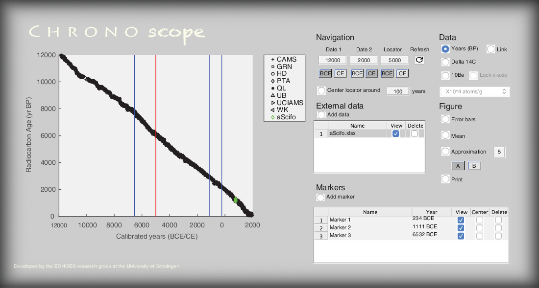
Figure 1 Software interface.
Data Types
On the top right side of the application, we introduce five radiobuttons. The user can use these to navigate between the three data types: 14C (yr BP), Δ14C (‰) and 10Be (X103 atoms/g or X104 atoms/g or X105 atoms/cm2/year (flux)). The “link” radiobutton will plot the two data types of 14C and Δ14C in a subplot. The legend of the 10Be, is interactive. All the data types that are illustrated can be selected or de-selected with a mouse click on their name in the legend. The ones that are de-selected are not shown in the figure. The x-axis can stay at its current limits by choosing the “Lock x-axis” radiobutton on the right. If this button is de-selected, the axis will be rescaled to the new range of the data that are plotted.
Data Processing and Visualization
The radiocarbon data typically have a 1 σ uncertainty expressed around each value (y-axis). The sample frequency (x-axis) is usually between 5 and 10 years, and on some occasions interpolation is needed. Another particularity of these datasets is that for the same years there are sometimes multiple values. This is because measurements are done by several laboratories that use trees from different parts of the world.
In CHRONOscope, in the “Figure” panel, one can visualize the uncertainty in the data by setting the “Error bars” radiobutton to “true” mode. In the same panel, we introduce the functions “Mean” and “Approximation”. The functions interpolate the data linearly and non-linearly, respectively. One example of how the error bars and the approximations are shown in the application is illustrated in Figure 2. We call the linear interpolation “Mean” because before the interpolation, we compute an average between the highest and the lowest error values of the respective highest and the lowest data points, where multiple values occur. In the “Approximation” function we apply the “spline” non-linear interpolation method Reinsch (Reference Reinsch1967). We provide the option for the user to set some interpolation parameters manually, such as the number of breaks (resolution) that are used by the spline, and which data points are to be considered by the method. In the “Figure” panel below the “Approximation”, we provide two options for the number of data points to be approximated. In option “A” we consider the entire dataset, while in option “B” we consider only the ones that are shown in the plot.
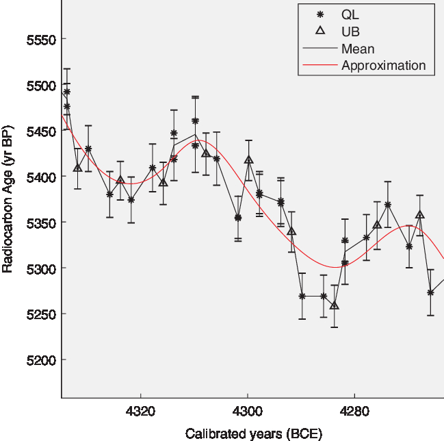
Figure 2 Example of how the error bars and the approximations are shown in the interface.
In this panel there is an option to print the current plot in an external figure and to save the plot in any available MATLAB graphics format.
External Data
In the “External data” panel, the user can import other data of their own. These data have to be in Microsoft Excel format and are uploaded from the menu (File / Import / Data). The data in the Microsoft Excel file should have the form described in the example shown in Table 1. The data here have been acquired by the Center for Isotope Research in the University of Groningen, Scifo (Reference Scifo2017).
Table 1 Example on how the data should be ordered in the Microsoft Excel file for importing them to the CHRONOscope. These data have been acquired in the Center for Isotope Research at the University of Groningen.

A list of external data is shown in the same panel, where the user has the option to superimpose them on IntCal13 or to remove them entirely.
The data that are shown in the figure, including the interpolations, can be exported using File / Export / Data. They will be saved in Microsoft Excel format.
Markers
In the “Markers” panel, one can add markers for quick navigation between data of interest. The markers are shown in the Figure panel as vertical blue lines. A list of markers is shown in the same panel and the user can navigate between them by choosing the respective buttons on this list. The list of markers can be exported using File / Export / Markers.
CONCLUSIONS
CHRONOscope is a useful tool for the visualization and processing of atmospheric 14C, Δ14C and 10Be data and it can be used in a wide range of analyses.
ACKNOWLEDGMENTS
This work is funded by an ERC research project (ECHOES) with grant number 714679.


 Open access