


1. Introduction
Mild-slope equations (MSE) address the problem of linearly propagating waves in an irrotational flow of an incompressible, inviscid, homogeneous fluid. These equations describe the combined effect of diffraction and refraction of linear surface waves propagating over a variable bathymetry. The waves being addressed are monochromatic and therefore a narrow wavenumber spectrum is achieved. This justifies the use of an approximate vertical velocity profile in order to reduce the original three-dimensional (3-D) problem to a two-dimensional (2-D) one.
The original mild-slope assumption states that the change in the water depth over the wave wavelength is small. This assumption is represented by the introduction of a small parameter into the equations, allowing higher-order terms in the bottom slope and curvature to be discarded. This approach was introduced by Berkhoff (Reference Berkhoff1973, Reference Berkhoff1976). An MSE is introduced by a vertical-averaging procedure to reduce the governing equations of the full 3-D problem to the depth-integrated equations in the horizontal plane. The vertical structure utilized fits that of waves on a horizontal bottom.
The MSE may be unsuccessful in producing adequate approximations to certain types of topography, such as rippled beds, which present higher-order phenomena due to steeper bottom slopes. Equations with higher-order bottom derivatives are required to overcome this difficulty.
Chamberlain & Porter (Reference Chamberlain and Porter1995) addressed this issue by adding the second-order bottom derivative terms which were neglected in the MSE. The same vertical profile of the velocity field is assumed and, when averaged over the depth, the second-order terms in derivatives of the depth  $(\nabla ^2 h$ and $(\nabla h)^2)$ are retained. This equation, which is referred to as the modified MSE (MMSE), successfully predicts known scattering phenomena which were undetected by Berkhoff by retaining the higher-order terms. These second-order terms were first introduced by Smith & Sprinks (Reference Smith and Sprinks1975). Miles & Chamberlain (Reference Miles and Chamberlain1998) expanded the MMSE and derived a fourth-order equation. Porter (Reference Porter2003) used transformation of variables to derive a model that accounted for Bragg scattering using only first-order bottom derivatives.
Kirby (Reference Kirby1986) addressed the problem of nearly resonant Bragg scattering due to small oscillatory depth variations around a mildly sloped reference depth. The same vertical structure of the velocity field was employed along with Green's second identity for a vertical-averaging technique. The resulting equation is applicable both to the case of resonant scattering by an undulating bottom and to the case of slow, non-resonant scattering. The scattering is defined by detuned undulations or by the slow change in the average depth, which is important in the absence of strong resonant scattering. The emphasis of the equation is for small deviations in relation to the wave amplitude on a mean, slowly varying depth.
All the equations mentioned so far take the potential function as the unknown which is to be determined. Kim & Bai (Reference Kim and Bai2004) derived an MSE in terms of the streamfunction vector. In this formulation, referred to as the complementary MSE (CMSE), the bottom condition is satisfied exactly and not only on a horizontal bottom as in the potential formulations. The continuity equation and kinematic free-surface condition are satisfied as well while the irrotational condition is satisfied only in the averaged sense. The CMSE was shown to give a better agreement with exact linear theory compared with other mild-slope type equations. The drawback in this formulation is that a vector equation is derived for the general case. This was somewhat alleviated by Toledo & Agnon (Reference Toledo and Agnon2010) who formulated an equivalent scalar equation to the vector equation using a pseudo-potential formulation. The equation performed especially well for sinusoidal beds and bottom mounds and is an efficient tool to predict wave diffraction over steep bathymetries. A unified approach to MSE was recently presented by Porter (Reference Porter2020).
Ehrenmark (Reference Ehrenmark2005) derived an improved linear dispersion relation which accounts for the first-order bottom slope as well as for the depth. The relation is derived from an asymptotic analysis of the exact solution of the linear wave problem combined with the method of steepest descent.
The modified dispersion relation appears to have significantly increased accuracy over sloping beds when tested on the plane beach problem with various forms of the MSE (Ehrenmark & Williams Reference Ehrenmark and Williams2010). It provides a global error reduction of the order of 50 per cent in some ‘from deep to shore’ computations. Specifically, this dispersion relation is utilized to obtain modified coefficients in the MMSE for the case of small bottom slopes. Belibassakis & Athanassoulis (Reference Belibassakis and Athanassoulis2006) have addressed normally incident waves on a sloping plane beach using polar coordinates. By doing so they have derived the modified dispersion relation and a polar MSE, exhibiting very good agreement with exact solutions.
In this paper, the steps to derive a 3-D MSE in cylindrical-Cartesian coordinates on a sloping plane beach are outlined. In addition, a quasi-3-D equation of oblique incidence is derived along with a 2-D MSE in polar-Cartesian coordinates. All equations are derived as a function of the streamfunction. The advantage of using the cylindrical coordinates is that the profile is formulated by using the boundary conditions at the bottom given as a constant-angle line, whereas the Cartesian coordinate formulation is a better fit for the bottom located along a horizontal line. This is a significant distinction since it increases the order of the bottom slope contribution in the formulation while maintaining the same order of expansion to the equation. This is manifested in the 2-D polar linear dispersion relation which is a function of the bottom slope to first order, as well as the bottom location as first derived by Ehrenmark (Reference Ehrenmark2005).
The streamfunction vertical profile is constructed based on the polar coordinate formulation. A combined polar-Cartesian (PC) MSE (PCMSE) is then derived by taking a variation of the Lagrangian functional. The functional represents the energy of the system and is generally equal to the difference between its kinetic and potential energies. Hamilton's principle states that the solution to the equations of motion is obtained where the time-averaged Lagrangian has a stationary value for the solutions satisfying the kinematic constraints. The equation is developed in § 2 by taking variations of the Cartesian Lagrangian formulation while substituting the polar vertical profile to the variables. Finally, the PCMSE is compared with the benchmark MSE models in § 3 for several test cases. Conclusions are drawn in § 4.
2. Mathematical formulation
In the following subsections, the vertical profile of a two-component vector streamfunction in a 3-D fluid domain, is determined. The vector function represents an extension to the 2-D streamfunction and is derived by using the cylindrical coordinate formulation. In this formulation, the flow domain is subdivided into stripes of constant-radius arcs which connect the corresponding points on the free surface and the bottom. The bottom gradient defines the arc function and the corresponding linear mean free-surface point. This approach was used successfully by Belibassakis & Athanassoulis (Reference Belibassakis and Athanassoulis2006) who derived a polar MSE and applied it to a wedge geometry with a constant slope. However, on a non-planar beach, when stratifying the fluid domain in this manner, there are crossings and overlaps between different arcs depending on the bottom gradient in the region. This results in a solution which is not determined continuously along the flow direction, but in a more sporadic manner. In addition, some free-surface regions will have a stronger impact than others. Due to this, we found that a cylindrical MSE does not provide good results for a general bathymetry. In order to overcome this difficulty and still exploit the advantages of the cylindrical representation, only the vertical profile of the vector streamfunction is determined using cylindrical coordinates. This profile is then translated to an equivalent Cartesian profile for the remainder of the solution.
In § 2.1, the cylindrical vertical profile is presented. In § 2.2 we derive the 2-D PCMSE and in § 3.3, the quasi-3-D equation for obliquely incident waves.
2.1. The angular profile
2.1.1. Cylindrical coordinates – problem definition
The governing equations and boundary conditions are presented in cylindrical coordinates in order to provide an approximate angular profile for the two-component vector streamfunction in a 3-D fluid domain. This domain is contained in the polar plane for which  $r$ and $\theta$ are the radial distance and the angle, respectively, and the longitudinal $y$-axis is normal to the polar plane. The ray $\theta =0$ represents the mean location of the free surface, and $r=0$ corresponds to the shore, as depicted in figure 1.

Figure 1. Polar coordinates – problem description.
Introducing the complex-valued vector streamfunction
 \begin{equation} \boldsymbol{\boldsymbol{\varPsi}}(x,y,z) \equiv \int_{{-}h}^z \boldsymbol{u}(x,y,z_0) \,{\rm d} z_0, \end{equation}
which defines the time harmonic streamfunction by  ${\rm Re}(\boldsymbol {\varPsi } \exp ({-{\rm i}\omega t}))$, with $\omega$ being the angular frequency of the incoming wave, and $z=-h$ being the location of the bottom. The horizontal and vertical velocity components are denoted by $\boldsymbol {u}$ and $w$, respectively, and are determined via
 \begin{equation} \boldsymbol{u} = \frac{\partial \boldsymbol{\varPsi}}{\partial z},\quad w ={-}\boldsymbol{\nabla} \boldsymbol{\cdot} \boldsymbol{\varPsi}, \end{equation}
with  $\boldsymbol {\nabla } = ({\partial }/{\partial x}, {\partial }/{\partial y})$. The vector streamfunction $\boldsymbol {\varPsi }$ satisfies the Laplace equation formulated in cylindrical coordinates in the flow domain
 \begin{gather} \frac{1}{r} \frac{\partial}{\partial r} \left( r \frac{\partial \boldsymbol{\varPsi}}{\partial r} \right) + \frac{1}{r^2} \frac{\partial^2 \boldsymbol{\varPsi}}{\partial \theta^2}+ \frac{\partial^2 \boldsymbol{\varPsi}}{\partial y^2}= 0 \quad {\rm in}\ 0< r<\infty,\quad -\alpha<\theta<0,\enspace -\infty< y<\infty. \end{gather}
The bottom boundary condition is formulated in terms of the vector streamfunction (2.1)
 \begin{equation} \boldsymbol{\varPsi} = 0 \quad {\rm at}\ \theta ={-}\alpha, \end{equation}
and the Cartesian free-surface condition is translated to cylindrical coordinates. At the undisturbed free surface
 \begin{equation} r {\rm d} \theta = {\rm d} z \rightarrow \frac{1}{r} \frac{\partial \boldsymbol{\varPsi}}{\partial \theta} = \frac{\partial \boldsymbol{\varPsi}}{\partial z},\quad \boldsymbol{\nabla} \boldsymbol{\cdot} \boldsymbol{\varPsi} = \boldsymbol{\nabla}_{cy} \boldsymbol{\cdot} \boldsymbol{\varPsi}, \end{equation}
with  $\boldsymbol {\nabla }_{cy} = ({\partial }/{\partial r},{\partial }/{\partial y})$.
These relations are then substituted into the boundary condition to be satisfied at the undisturbed location  $z=0$ of the free surface. These conditions arise from the minimization of the energy functional (Kim & Bai Reference Kim and Bai2004) in terms of the vector streamfunction $\boldsymbol {\varPsi }$. They are then written in the Cartesian frame in order to derive the equivalent cylindrical condition
 \begin{equation} \frac{\partial \boldsymbol{\varPsi}}{\partial z} +\frac{1}{\sigma} \boldsymbol{\nabla} (\boldsymbol{\nabla}\boldsymbol{\cdot} \boldsymbol{\varPsi}) = 0 \quad {\rm at}\ z = 0, \end{equation}
where  $\sigma \equiv {\omega ^2}/{g}$. In cylindrical coordinates, (2.6) is written as
 \begin{equation} \frac{1}{r} \frac{\partial \boldsymbol{\varPsi}}{\partial \theta} + \frac{1}{\sigma} \boldsymbol{\nabla}_{cy} (\boldsymbol{\nabla}_{cy} \boldsymbol{\cdot} \boldsymbol{\varPsi})= 0 \quad {\rm at} \theta = 0. \end{equation}
Equations (2.3)–(2.7) constitute a closed set of equations to find a solution for the vector streamfunction  $\boldsymbol {\varPsi }$, when supplemented by lateral boundary conditions. This solution can then be utilized to determine the free-surface location by resolving it from the kinematic boundary condition
 \begin{equation} \eta = \frac{1}{{\rm i} \omega} \boldsymbol{\nabla}_{cy} \boldsymbol{\cdot} \boldsymbol{\varPsi} \quad {\rm at}\ \theta = 0. \end{equation}
2.1.2. The  $\theta$-dependent profile

The set of equations (2.3)–(2.7) is solved by assuming a solution to the vector streamfunction,  $\boldsymbol {\varPsi }$, in a separable form. It is noted that this variable separation will provide an approximate solution to the problem when solved on the cylinder segment. The segment is composed of a circle sector in the polar plane, defined between the free surface and the planar bottom and along the shore in the longitudinal plane
 \begin{equation} \boldsymbol{\varPsi}(r,\theta,y) = \sum_{n=0}^{\infty} R_n(r) F_n(\theta) Y_n(y), \end{equation}
and  $F_n(\theta )$ will be utilized as the approximation for the angular profile of the vector streamfunction.
Substituting this expression into (2.3) yields
 \begin{equation} \left.\begin{gathered} \frac{1}{F_n} \frac{{\rm d}^2 F_n}{{\rm d} \theta^2} = \gamma_n^2,\\ \frac{1}{Y_n} \frac{{\rm d}^2 Y_n}{{{\rm d}y}^2} ={-}\delta_n^2,\\ \frac{{\rm d}^2 R_n}{{\rm d} r^2} + \frac{1}{r} \frac{{\rm d} R_n}{{\rm d} r} + \left(\frac{\gamma_n^2}{r^2} - \delta_n^2\right)R_n = 0, \end{gathered}\right\} \end{equation}
where  $\gamma _n$ and $\delta _n$ are positive constants, analogous to the components of the vector wavenumber $k$, normally used in the Cartesian formulation.
Defining the solution around a local wavenumber expressed by the constants  $\gamma _n$ and $\delta _n$, an oscillating solution is chosen in the $y$ direction. In the $r$ direction, Bessel functions are obtained. The solution in the angular direction has exponential form
 \begin{equation} F(\theta) = A \sinh({\gamma \theta}) + B \cosh({\gamma \theta}). \end{equation}
This solution is then substituted into the boundary condition at the bottom and then normalized with the value at the free surface ( $\theta =0$) to yield
 \begin{equation} F(\theta) = \frac{\sinh(\gamma(\theta+\alpha))}{\sinh(\gamma \alpha)}. \end{equation}
The  $\sinh (\gamma (\theta +\alpha ))$ shape will serve in what follows as an approximated profile and will be utilized to derive the mild-slope equation in the horizontal direction.
This profile is then substituted into the time-averaged cylindrical Lagrangian in order to provide a solution for the case of a 3-D planar beach
 \begin{equation} \left.\begin{gathered} \bar{L} = \int \int L \,{\rm d} r \,{{\rm d}y},\\ \bar{L} = \frac{\rho}{2} \int_{-\alpha}^0 \left(|\boldsymbol{\nabla}_{cy} \boldsymbol{\cdot} \boldsymbol{\varPsi}|^2 + \frac{1}{r^2} \left|\frac{\partial \boldsymbol{\varPsi}}{\partial \theta}\right|^2 \right) r \,{\rm d}\theta - \frac{\rho}{2 \sigma} |\boldsymbol{\nabla}_{cy} \boldsymbol{\cdot} \boldsymbol{\varPsi}(r,y,0)|^2. \end{gathered}\right\} \end{equation}
Here,  $L$ is the Lagrangian density and the double integration is made in the domain defined by lateral boundary conditions which appropriately depict the problem at hand. Since the wave field is harmonic, the (quadratic) Lagrangian has a zeroth harmonic component and a second harmonic one. Hence, there are two alternative applications of the Lagrangian: the present, time-averaged component, utilized by Kim & Bai (Reference Kim and Bai2004), or the oscillatory component, utilized by Chamberlain & Porter (Reference Chamberlain and Porter1995).
The extension of this formulation to a full 3-D bathymetry will be provided in future work.
For the case of a general 2-D bathymetry, the Cartesian equivalent to the angular profile is substituted into the Cartesian Lagrangian
 \begin{equation} \left.\begin{gathered} \bar{L} = \int L {{\rm d}x},\\ L = \frac{\rho}{2} \int_{{-}h(x)}^0 \left(\left|\frac{\partial \boldsymbol{\varPsi}}{\partial x}\right|^2 + \left|\frac{\partial \boldsymbol{\varPsi}}{\partial z}\right|^2 \right) {\rm d} z - \frac{\rho}{2 \sigma} \left|\frac{\partial \boldsymbol{\varPsi}(x,0)}{\partial x}\right|^2, \end{gathered}\right\} \end{equation}
after which the first variation is equated to zero to derive a 2-D MSE.
2.2. The 2-D PC mild-slope equation
In two dimensions, the problem is constructed in the polar plane and the vector streamfunction reduces to a scalar streamfunction  $\boldsymbol {\varPsi } = (\psi,0)$. The set of equations (2.3)–(2.7) reduces to
 \begin{gather} \frac{1}{r} \frac{\partial}{\partial r} \left(r \frac{\partial \psi}{\partial r} \right) + \frac{1}{r^2} \frac{\partial^2 \psi}{\partial \theta^2} = 0 \quad {\rm in}\ 0< r<\infty,\quad -\alpha<\theta<0. \end{gather}
 \begin{gather}\psi = 0 \quad {\rm at}\ \theta ={-}\alpha, \end{gather}
 \begin{gather}\frac{1}{r} \frac{\partial \psi}{\partial \theta} +\frac{1}{\sigma} \frac{\partial^2 \psi}{\partial r^2}= 0 \quad {\rm at}\ \theta = 0. \end{gather}
The solution form for variable separation around a local wavenumber
 \begin{gather} F(\theta) = A \sinh(\gamma {\theta}) + B \cosh({\gamma \theta}), \end{gather}
 \begin{gather}R(r) = C \cos(\gamma \ln r) + D \sin(\gamma \ln r), \end{gather}
where the constants are determined by substitution into the boundary conditions. A localized dispersion relation is derived when substituting the solution form into the free-surface boundary condition (2.17)
 \begin{equation} \sigma r = \gamma \tanh(\gamma\alpha). \end{equation}
This is simply a reconstruction of the relation derived by Ehrenmark (Reference Ehrenmark2005), as stated above.
When solving for a general bathymetry, the local bed gradient defines the angle  $\alpha$. The origin of the polar reference frame is located where the corresponding ray intersects with the line of the undisturbed free surface. Therefore, at each local point the axis origin shifts according to the bottom gradient.
The relations between the polar and Cartesian parameters, as depicted in figure 2, are provided by the following:
 \begin{equation} \theta = \arctan\left(\frac{z h'}{h}\right),\quad \alpha = \arctan(h'). \end{equation}
The following form of  $\psi$ is substituted into the Lagrangian
 \begin{equation} \psi(r,\theta) = \psi_0(r) F(\theta), \end{equation}
and the problem is then to be solved for the unknown function  $\psi _0(r)$.

Figure 2. Polar-Cartesian relations.
The Cartesian equivalent profile of (2.12) is given by
 \begin{equation} F \left(h(x),h'(x),z \right) = \frac{\sinh\left(\gamma \left(\arctan\left(\dfrac{z h'}{h}\right) + \arctan(h') \right)\right)}{\sinh \left(\gamma \arctan(h') \right)}. \end{equation}
A solution for  $\psi (x,z)$ is sought in the form of
 \begin{equation} \psi(x,z) = \psi_0(x) F \left(h(x),h'(x),z \right). \end{equation}
Substituting the profile into the Lagrangian (2.14), yields
 \begin{equation} L = \left(a - \frac{1}{\sigma} \right) | \psi_{0_x} |^2 + (c+d) | \psi_0 |^2 + 2b \,{\rm Re} \left(\psi_0 \psi_{0_x}^* \right), \end{equation}
where  $\textrm {Re}(x)$ denotes the real part of $x$,
$x$,  $*$ denotes the complex conjugate and the coefficients $a,b,c$ and $d$ are real-valued functions of $h(x)$ and $h'(x)$ defined by
 \begin{equation} a = \int_{{-}h}^0 F^2 \,{\rm d} z \quad b = \int_{{-}h}^0 F F_x \,{\rm d} z \quad c = \int_{{-}h}^0 F_x^2 \,{\rm d} z \quad d = \int_{{-}h}^0 F_z^2 \,{\rm d} z. \end{equation}
 Following the substitution, the Lagrangian becomes a functional of a single variable,  $\psi _0$, and the Euler–Lagrange equation is derived in the form
 \begin{equation} -\left[ \left(a-\frac{1}{\sigma}\right) \psi_{0_{x}} + b \psi_{0} \right]_x + b \psi_{0_x} + (c+d) \psi_0 = 0. \end{equation}
Its solution will provide the stationary point of the Lagrangian and the solution to the original system of equations. Note that the coefficients of (2.27) depend on  $x$, so the $b$-term does not cancel out.
This is the PCMSE and the main result presented in the paper. The structure of the equation is similar to that of the CMSE and the fundamental difference is in the order of the bottom derivative in the coefficients. This is up to third order here as opposed to second order in the CMSE.
We note that numerical issues arise with evaluation of the coefficients  $a,b$ and $c$ defined in (2.26a–d) when solving (2.27) in a horizontal or close to horizontal bed. The values of $\alpha$ and $\theta$ both tend to zero at the limit where $h^\prime \to 0$. In order to obtain a smooth solution in the entire range from a steep slope to a horizontal bottom, the variables are normalized in the following form:
 \begin{equation} \alpha_0 = \alpha r_0,\quad \theta_0 = \theta r_0,\quad \gamma_0 = \frac{\gamma}{r_0},\quad r_0 \equiv \frac{h}{h^\prime}. \end{equation}
Under this transformation, the vertical velocity profile remains unchanged. The polar coordinate variables reduce to the equivalent Cartesian variables in the limit of a horizontal bottom, and this resolves the numerical complications
 \begin{equation} \lim_{h^\prime \to 0} \alpha_0 = h,\quad \lim_{h^\prime \to 0} \theta_0 = z, \end{equation}
and the polar dispersion relation reduces to its Cartesian version
 \begin{equation} \sigma = \gamma_0 \tanh(\mu \gamma_0 h),\quad \mu \equiv \alpha \cot(\alpha),\quad \lim_{h^\prime \to 0} \mu = 1. \end{equation}
This representation reduces the PCMSE to the CMSE for bottom slopes which tend to zero. Effectively, this means that when solving horizontal or close to horizontal bottom profiles the CMSE and PCMSE will provide similar results. For relatively steep gradients the results will differ according to the coefficient terms of each equation.
In terms of the normalized variables, the streamfunction profile is now given as
 \begin{equation} F(\gamma_0,h,h^\prime) = \frac{\sinh\left[\gamma_0(\theta_0+\alpha_0)\right]}{\sinh(\gamma_0\alpha_0)} = \frac{\sinh\left[\dfrac{\gamma_0 h}{h^\prime}\left(\arctan\left(\dfrac{z h^\prime}{h}\right) + \arctan(h^\prime) \right)\right]}{\sinh \left(\dfrac{\gamma_0 h}{h^\prime} \arctan(h^\prime) \right)}. \end{equation}
This profile and its derivatives are integrated with respect to the vertical coordinate in order to obtain the coefficients of (2.27). Due to the complexity of the terms derived by analytical integration, this task is accomplished in two ways. The first one is by a Taylor expansion, assuming a small  $\alpha$, which reduces the complexity of the terms derived from the analytical integration. The challenge is that using $\alpha$ as the expansion parameter requires taking several orders to obtain values that warrant a satisfactory approximation. This leads to lengthy and cumbersome expressions. To overcome this difficulty and to simplify the coefficients resulting from (2.26a–d), the following parameter is utilized:
 \begin{equation} p \equiv 1-\mu. \end{equation}
With  $p$ as the expansion parameter, accurate simulations are derived by expanding (2.31) to first order. Also, $\alpha$ is expanded into powers of $p$ by using successive approximations $\alpha = \sqrt {3 p} (1-{p}/{10} + O(p^2) )$ and subsequently used in the integration (2.26a–d) to obtain the coefficients of the PCMSE. The coefficient terms to first order in $p$ are provided in Appendix A. This is referred to in the following as the PCMSE.
The second is by numerical integration of the full coefficients in what will be referred to as the ‘steep-slope’ equation. In this equation, no approximations have been imposed on the bottom slope and therefore it exceeds the mild-slope approximation and provides a first ‘steep-slope’ equation. This is referred to in the following as the PCSSE (PC steep-slope equation).
2.3. The quasi-3-D equation of oblique incidence
The case of an incoming wave which is incident to the bottom gradient at a varying angle is considered. A local axis system is defined such that the  $x$ axis is oriented in the direction of the gradient at each point. The PC vertical profile is utilized in this direction of varying depth topography (2.31). This profile is denoted as $f_1$ in the following derivation. The corresponding local $y$ axis is that of a horizontal bottom which specifies a harmonic solution dependence. The profile in this direction is defined as
 \begin{equation} f_2 = \frac{\sinh\left(\gamma_0(z+h)\right)}{\sinh(\gamma_0 h)}. \end{equation}
Where  $\gamma _0$ is the solution of the PC dispersion relation (2.30a–c), as stated previously. The vector streamfunction is approximated by a separation of variables. This is expressed as a multiplication of a $y$ dependent harmonic function, an approximated vertical profile and an unknown horizontal function. The horizontal function represents the stream value at the undisturbed free surface
 \begin{equation} \boldsymbol{\varPsi}(x,y,z) = \exp({{\rm i} \beta_0 y}) \left(f_1(h,h',z) \psi_1(x), f_2(h,z) \psi_2(x)\right), \end{equation}
with  $\beta _0$ being the $y$ component of the wavenumber vector. This is then substituted into the 3-D time-averaged Lagrangian
 \begin{equation} L = \int_{{-}h}^0 \left( | u |^2 + | v |^2 + | w |^2 \right) {\rm d} z - g |\zeta|^2, \end{equation}
where  $u,v$ and $w$ are the complex-valued local velocities in the $x,y$ and $z$ directions and $\zeta$ is the complex-valued free-surface location. The velocities are calculated according to the streamfunction definition
 \begin{equation} \left.\begin{gathered} {}[u,v] = \boldsymbol{\varPsi}_z = \exp({{\rm i} \beta_0 y}) \left(f_{1_z} \psi_1, f_{2_z} \psi_2 \right)\\ w ={-}\boldsymbol{\nabla} \boldsymbol{\cdot} \boldsymbol{\varPsi} ={-}\exp({{\rm i} \beta_0 y}) (f_{1_x} \psi_1 + f_1 \psi_{1_x} + {\rm i} \beta_0 f_2 \psi_2 ), \end{gathered}\right\} \end{equation}
and the free-surface location is calculated according to the kinematic linear free-surface condition
 \begin{equation} \zeta = \frac{1}{{\rm i}\omega} \boldsymbol{\nabla} \boldsymbol{\cdot} \boldsymbol{\varPsi}_0 = \frac{1}{{\rm i} \omega} \exp({{\rm i} \beta_0 y})(\psi_{1_x} + {\rm i}\beta_0 \psi_2). \end{equation}
These expressions are substituted into the Lagrangian
 \begin{align} L &= (c_1+d_1) | \psi_1 |^2 + a_2 (\beta_0^2 - \gamma_0^2) | \psi_2 |^2 + a_1 | \psi_{1_x} |^2 \nonumber\\ &\quad + 2 b_1 (\psi_1 \psi_{1_x}^* + \psi_1^* \psi_{1_x}) + {\rm i} \beta_0 b_{12} (\psi_2 \psi_1^* - \psi_1\psi_2^*) \nonumber\\ &\quad + {\rm i}\beta_0 a_{12} (\psi_2 \psi_{1_x}^* - \psi_{1_x} \psi_2^*), \end{align}
where
 \begin{equation} \left.\begin{gathered} a_1 = \int_{{-}h}^0 f_1^2 \,{\rm d} z - \frac{1}{\sigma} \quad b_1 = \int_{{-}h}^0 f_1 f_{1_x} \,{\rm d} z \quad c_1 = \int_{{-}h}^0 f_{1_x}^2 \,{\rm d} z\\ d_1 = \int_{{-}h}^0 f_{1_z}^2 \,{\rm d} z \quad a_2 = \int_{{-}h}^0 f_2^2 \,{\rm d} z - \frac{1}{\sigma} \quad a_{12} = \int_{{-}h}^0 f_1 f_2 \,{\rm d} z - \frac{1}{\sigma}\\ b_{12} = \int_{{-}h}^0 f_2 f_{1_x} \,{\rm d} z. \end{gathered}\right\} \end{equation}
Variations are taken with respect to both parameters,  $\psi _1$ and $\psi _2$, and equated to 0. The variation with respect to $\psi _2$ provides
 \begin{equation} \psi_2 = \frac{{\rm i} \beta_0 \left( b_{12} \psi_1 + a_{12} \psi_{1_x} \right)}{a_2 (\beta_0^2 - \gamma_0^2)} \equiv {\rm i}\beta_0 (r_1 \psi_1+r_2 \psi_{1_x}), \end{equation}
and with respect to  $\psi _1$, after substituting for $\psi _2$ and rearranging
 \begin{equation} \psi_{1_{xx}} + \frac{R_1}{L_1} \psi_{1_x} + \frac{R_2}{L_1} \psi_1 = 0 \end{equation}
where
 \begin{equation} \left.\begin{gathered} R_1 ={-}a_{1_x}-\beta_0^2(b_{12}-a_{{12}_x}) r_2 + \beta_0^2 a_{12} (r_1+r_{2_x})\\ R_2 = c_1+d_1-b_{1_x}-\beta_0^2(b_{12}-a_{{12}_x}) r_2 + \beta_0^2 a_{12} (r_1+r_{2_x})\\ L_1 ={-}a_1+\beta_0^2 a_{12} r_2. \end{gathered}\right\} \end{equation}
3. Simulations
Numerical results are presented for the simulation of four 2-D test cases in the following subsections: the Roseau bathymetry, a constant-slope bottom, a benchmark example known as Booij's ramp and a doubly sinusoidal bottom which allows us to test the case of a class II Bragg resonance. A simulation of the quasi-3-D case of obliquely incident waves is performed as well. The numerical simulations for all MSE models presented here are solved by using the NDsolve function of Mathematica and the ODE45 function of Matlab. The spatial step size is of the order of 0.01. These results are then presented along with the results of other benchmark MSE models in comparison with known analytical solutions of these test cases.
3.1. Roseau's bathymetry
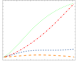
Roseau (Reference Roseau1976) derived the only analytical solution for waves propagating over a non-constant-slope bathymetry. In his solution, the bed location is defined by
 \begin{gather} \left.\begin{gathered} \frac{x(\xi)}{h_0} = \xi - (2 \varPi \beta)^{{-}1} \left(1-\frac{h_L}{h_0}\right) \ln \left(1+\exp({2\beta \varPi \xi}) + 2\exp({\beta \varPi \xi}) \cos(\beta \varPi) \right),\\ \frac{z(\xi)}{h_0} ={-}1 + (\varPi \beta)^{{-}1} \left(1-\frac{h_L}{h_0}\right) \arctan \left(\frac{\sin(\beta \varPi)}{\exp({-\beta \varPi \xi}) +\cos(\beta \varPi)} \right), \end{gathered}\right\} \end{gather}
where  $\beta \in (0,1)$ is a shoaling parameter and the bed is defined parametrically as $z(\xi ) = -h(x(\xi ))$. The bed function tends to two flat semi-infinite sections at the limits $x \to \pm \infty$, as depicted in figure 3.

Figure 3. Roseau's bed function for  ${h_L}/{h_0}=0.25$. The $x$ axis is the horizontal distance. The $z$ axis is the vertical location of the bottom. The values are normalized with respect to $h_0$. Green (dotted) curve – $\beta = 0.5$; red (dashed) curve – $\beta = 0.45$; blue (solid) curve – $\beta = 0.4$.
The reflection coefficient, defined as the ratio of the amplitude of a reflected wave to that of a corresponding incident wave, is as given by Roseau
 \begin{equation} | R| = \left| \frac{\sinh\left((k_0h_0-k_Lh_L)/\beta \right)}{\sinh\left((k_0h_0+k_Lh_L)/\beta \right)} \right|, \end{equation}
where  $k_0$ and $k_L$ are the wavenumbers at the constant depth locations, $h_0$ and $h_L$, respectively. A solution to the case of reflection and transmission of temporally harmonic waves as presented by Porter (Reference Porter2019) is utilized here. The waves are of frequency $\omega$, incident from $x=-\infty$ over a finite region of variable 2-D bathymetry between two flat semi-infinite sections defined by $h = h_0\ \textrm {at}\ x<0$ and $h = h_L\ \textrm {at}\ x>L$,
This method is applied to the MSE models and the reflection coefficient is solved for numerically. The results are presented in comparison with the exact solution of Roseau for three values of  $\beta$ and two relations between the depths at the flat regions ${h_L}/{h_0}$. The maximum slopes of the simulations which are presented here are $0.75,0.68$ and $0.62$ for $\beta = 0.5,0.45$ and $0.4$, respectively.
In addition, the conservation of energy flux (as presented by Massel Reference Massel1993) is tested for the steepest bathymetry case by equating net energy flux values on both sides of the variable region. This is stated by the following relation between the reflection and transmission coefficients and the relevant group velocity:
 \begin{equation} (C_g)_{h = h_0} (1-| R |^2) = (C_g)_{h = h_L} | T |^2 .\end{equation}
 Figure 4 displays the reflection coefficient  $R$ as a function of the non-dimensional $\sigma h_0$ for $\beta = 0.5$ for the CMSE, MMSE, PCMSE and the PCSSE in comparison with the analytical result of Roseau. In panel (b), $({h_l}/{h_0} = 0.25$) the results obtained from the PC equations are almost identical to the exact result and outperform the other models. In panel (a), ( ${h_l}/{h_0} = 0.1$) the differences are more significant and clearly the PC equations provide a better match than the other model equations. The PCSSE outperforms the PCMSE by a significant amount and is very close to the exact solution. In figure 5, the relative error ( $E_r = {(R_m-R_r)}/{R_r}$, where $R_m$ and $R_r$ are the MSE model and Roseau reflection coefficients, respectively) is presented for the PCMSE and PCSSE in comparison with the MMSE and CMSE (a,c) and with the MSE with the standard Cartesian dispersion relation and with Ehrenmark's dispersion relation (b,d) for $\beta = 0.5$ as well. The energy flux conservation (3.3) was tested for the case of ${h_L}/{h_0} = 0.25$. The maximum relative income–outcome energy flux value
 \begin{equation} \left(E_f = \frac{(C_g)_{h = h_0} (1-| R |^2) - (C_g)_{h = h_L} | T |^2}{(C_g)_{h = h_0} (1-| R |^2) + (C_g)_{h = h_L} | T |^2}\right), \end{equation}
is  $4\times 10^{-7}$ for all $\sigma h_0$ values which were tested. Figure 6 compares the relative error of the CMSE, MMSE and the PCMSE for $\beta$ values of $0.45$ and $0.4$. In panel (c), the PCMSE and the CMSE models provide indistinguishable results. The PCMSE can be seen to provide smaller relative errors in comparison with all models in an overall observation.

Figure 4. Simulation of the reflection coefficient vs  $\sigma h_0$ for the Roseau bathymetry. Here, $\beta = 0.5$. Panels show (a) ${h_L}/{h_0} = 0.1$, (b) ${h_L}/{h_0} = 0.25$. Blue (smaller dashed) curve – PCMSE; orange (larger dashed) curve – PCSSE; red (dot dashed) curve – CMSE; green (dotted) curve – MMSE; black (solid) curve - exact solution.

Figure 5. Simulation of the relative error vs  $\sigma h_0$ for the Roseau bathymetry. Here, $\beta = 0.5$. Panels show (a,b) ${h_L}/{h_0} = 0.1$, (c,d) ${h_L}/{h_0} = 0.25$. (a,c) Blue (smaller dashed) curve – PCMSE; orange (larger dashed) curve – PCSSE; red (dot dashed) curve – CMSE; green (dotted) curve – MMSE. (b,d) Blue (smaller dashed) curve – PCMSE; orange (larger dashed) curve – PCSSE; red (dot dashed) curve – MSE; green (dotted) curve – MSE with Ehrenmark's dispersion.

Figure 6. Simulation of the relative error vs  $\sigma h_0$ for the Roseau bathymetry. Panels show (a,c) ${h_L}/{h_0} = 0.1$, (b,d) ${h_L}/{h_0} = 0.25$, for (a,b) $\beta = 0.45$, (b,d) $\beta = 0.4$. Blue (smaller dashed) curve – PCMSE; orange (larger dashed) curve – PCSSE; red (dot dashed) curve – CMSE; green (dotted) curve – MMSE.
3.2. Constant-slope bathymetry
An exact solution to waves normally incident to the bottom gradient can be found in Stoker (Reference Stoker1957). The solution is limited to bottom slopes of  ${{\rm \pi} }/{2n}$, where $n$ is an integer. Simulations were performed for the bed slopes of $45,30,22.5,18$ and $15$ degrees. The analytical solution (Stoker Reference Stoker1957) is compared with the results of numerical simulations for the PCMSE, CMSE and a full polar MSE in figure 7 for slopes of $45^{\circ }$ and $30^{\circ }$ degrees. For $45^{\circ }$, the polar equation agrees slightly better than the PCMSE with the analytical result, and both provide better agreement than the CMSE, as observed in the figure. For $30^{\circ }$, all models are effectively indistinguishable from the exact solution, as is for all angles smaller than $30^{\circ }$. This strengthens the result from the previous test case for which the PCMSE has an advantage for steep slopes. The polar model, which is specifically designed for this test case, has a small advantage over the PC equations. The results of the CMSE matched those of the PC equations for milder slopes.

Figure 7. Normalized free-surface values for a normal incidence simulation for two values of the bed slope. Panels show (a)  $45^{\circ }$, (b) $30^{\circ }$. Blue (smaller dashed) curve – PCMSE; orange (larger dashed) curve – PCSSE; red (dot dashed) curve – CMSE; green (dotted) curve – polar MSE; black (solid) curve – exact solution.
3.3. Booij's ramp
The bed shape in the form of a ramp tested by Booij (Reference Booij1983) is simulated in what follows. The bathymetry is given by
 \begin{equation} h(x) = h_m - \left(\frac{h_p-h_m}{L}\right) x,\quad 0< x< L, \end{equation}
where  $h_m$ and $h_p$ are the constant depths upstream and downstream of the ramp, respectively. Following the studies by Kim & Bai (Reference Kim and Bai2004), we use the values
 \begin{equation} \frac{h_p}{h_m} = \frac{1}{3},\quad \frac{\omega^2 h_m}{g} = 0.6, \end{equation}
with the non-dimensional ramp length  ${\omega ^2 L}/{g}$ in the range between $0.1$ and $5$. In figure 8, the values of the reflection coefficient obtained using the PCMSE, CMSE and MMSE are compared with the result of the full linear theory of Bai & Yeung (Reference Bai and Yeung1974) using the localized finite-element method. The CMSE was solved in the domain containing the two points of a discontinuous bed slope by using the jump conditions suggested by Kim & Bai (Reference Kim and Bai2004). The PCMSE was solved using the same jump conditions extended to include the second-order slope discontinuity, as detailed below.

Figure 8. Comparison of the reflection coefficient derived using the exact solution and computed using various model equations for Booij's ramp. Blue (smaller dashed) curve – PCMSE; orange (larger dashed) curve – PCSSE; red (dot dashed) curve – CMSE; green (dotted) curve – MMSE; black (solid) curve – exact solution.
The streamfunction solution over the horizontal bed on both sides of the ramp is provided by (43) and (44) in Kim & Bai (Reference Kim and Bai2004) as
 \begin{equation} \left.\begin{gathered} \psi_0(x) \equiv \psi_0^-(x) = \frac{\omega A}{k_m}(\exp({{\rm i}k_mx})-R\exp({-{\rm i}k_mx})),\quad x<0,\\ \psi_0(x) \equiv \psi_0^+(x) = \frac{\omega A}{k_p}T\exp({{\rm i}k_px}),\quad x>L, \end{gathered}\right\} \end{equation}
with  $T$ being the amplitude-transmission coefficient, $k_m$ and $k_p$ are the wavenumbers of the wave upstream and downstream of the ramp, respectively. At the points of discontinuity in the bottom slope, namely, $x=0$ and $x=L$, a continuity of both $(a-{1}/{\sigma }) \psi _{0_{x}} + b \psi _{0}$ and $\psi _0$ is required
 \begin{equation} \left.\begin{gathered} \psi_0 = \psi_0^-,\quad \left(a(h^-, {h^\prime}^+)-\frac{1}{\sigma}\right) \psi_{0_{x}} + b(h^-, {h^\prime}^+,{h^{\prime \prime}}^+) \psi_{0} \\ =\left(a(h^-,0)-\frac{1}{\sigma}\right) \psi_{0_{x}}^- \quad {\rm at}\ x=0,\\ \psi_0 = \psi_0^+,\quad \left(a(h^+, {h^\prime}^-)-\frac{1}{\sigma}\right) \psi_{0_{x}} + b(h^+, {h^\prime}^-,{h^{\prime \prime}}^-) \psi_{0} \\ =\left(a(h^+,0)-\frac{1}{\sigma}\right) \psi_{0_{x}}^+ \quad {\rm at}\ x=L, \end{gathered}\right\} \end{equation}
equating the terms on both sides of the discontinuity points. The  $(+)$ and $(-)$ signs indicate taking a limit downstream and upstream of the discontinuity. Normalizing and substituting the streamfunction solution in the flat region into the equations above yields
 \begin{gather} \psi_{0_x} + \left({\rm i}k_m \frac{a(h^-,0)-\dfrac{1}{\sigma}}{a(h^-, h'^+)-\dfrac{1}{\sigma}} + \frac{b(h^-, h'^+,h''^+)}{a(h^-, h'^+)-\dfrac{1}{\sigma}} \right) \psi_0 = 2{\rm i}\omega A \frac{a(h^-,0)-\dfrac{1}{\sigma}}{a(h^-, h'^+)-\dfrac{1}{\sigma}},\quad x=0, \end{gather}
 \begin{gather}\psi_{0_x} - \left(ik_p \frac{a(h^+,0)-\dfrac{1}{\sigma}}{a(h^+, h'^-)-\dfrac{1}{\sigma}} + \frac{b(h^+, h'^-,h''^-)}{a(h^+, h'^-)-\dfrac{1}{\sigma}}\right) \psi_0 = 0,\quad x=L. \end{gather}
These are the jump conditions utilized in the numerical solution of the PCMSE.
Figure 8 demonstrates that the reflection coefficient obtained using the PCMSE shows a better agreement with the exact solution than that obtained using the CMSE in the range  ${\omega ^2 L}/{g}<0.6$. The MMSE provides the best results in this region. All models are almost indistinguishable in the rest of the region. This result shows yet again the compatibility of the PCMSE to the CMSE for milder slopes and a clearly improved solution for steeper slopes. All in all, the PCMSE solution provides a relatively good agreement in the entire region. It is noted that the left edge of the figure depicts very large bottom slopes which are outside the scope of relevance of these models.
3.4. Bragg resonance – class II
Bragg resonance refers to the interaction of free-surface incident waves with periodic bottom undulations satisfying resonant conditions. This phenomenon plays an important role in the evolution of nearshore waves. The class I Bragg resonance involves interactions of two surface waves and one bottom undulation satisfying the conditions
 \begin{equation} \left.\begin{gathered} k_1-k_2-k_b = 0,\\ \omega_1 - \omega_2 = 0. \end{gathered}\right\} \end{equation}
The subscript indices refer to the number of the free-surface wave, whereas  $b$ refers to the bed. This type of resonance has a significant effect on linear waves. The class II Bragg resonance involves the interaction of two surface waves and two bottom undulations satisfying the conditions
 \begin{equation} \left.\begin{gathered} k_1-k_2-(k_{b_1} \pm k_{b_2}) = 0,\\ \omega_1 - \omega_2 = 0. \end{gathered}\right\} \end{equation}
This type of resonance has a weaker effect on linear waves than the class I Bragg resonance, but can still have significant effects due to undulating bottom components. The classical MSE, which account for second-order terms, generally provide a good agreement with the class I Bragg resonance. On the other hand, they fail to capture the results of the higher-order conditions of the class II and higher.
The consideration of higher-order bed slopes in the PCMSE is expected to provide a better match to the class II Bragg resonance as compared with the classical MSE. The leading-order term for this class in the bottom slope is the  $(\nabla h)^2$ term. The comparison is performed below for small values of the dispersion parameter, $kh$, which is where the PCMSE equation is expected to provide the most accurate results.
Figures 9 and 10 depict the simulation results for the PCMSE, CMSE and MMSE in modelling the class II Bragg resonance reflection coefficient  $R$ on a doubly sinusoidal bottom as a function of $\sigma h_0$. The range of $\sigma h_0$ values is $0.02$ to $0.58$ in figure 10 which is within the range where the PCMSE is expected to work well. The range in figure 9 is $0.35$ to $2.15$ which extends well beyond this range and is therefore expected to provide more of a challenge to the models. The simulations of the MSE models are compared with the ‘linear exact’ result, as displayed in figure 3 of Kim et al. (Reference Kim, Ertekin and Bai2010) in figure 9. The first peak located at ${2 k}/{k_{b_1}} \approx 0.3$ in the figure is a result of the class II Bragg resonance. The result of the PCMSE is significantly closer to the linear exact result than the CMSE. The MMSE provides the closest value for this peak. It is noted that Kim et al. (Reference Kim, Ertekin and Bai2010) obtained slightly different results for the CMSE which are closer to the PCMSE results presented here.

Figure 9. Comparison of the values of the reflection coefficient  $R$ obtained from simulations of the analytical PCMSE (blue – smaller dashed curve), PCSSE (orange – larger dashed curve), CMSE (red – dot dashed curve) and MMSE (green – dotted curve) along with the result arising from the ‘linear exact’ solution presented by Kim, Ertekin & Bai (Reference Kim, Ertekin and Bai2010) (black – solid curve) taken from figure 3 there. The bed wavenumbers are $k_{b_1} = 2 {\rm \pi}$ cm $^{-1}$ and $k_{b_2} = {4 {\rm \pi}}/{3}$ cm $^{-1}$. The patch length is $L = 12$ cm, the amplitude ratio is ${{\rm \Delta} H}/{H_0} = 0.25$ and $H_0 = 2.5$ cm.

Figure 10. Comparison of the values of the reflection coefficient  $R$ obtained from simulations of the analytical PCMSE (blue – smaller dashed curve), PCSSE (orange – larger dashed curve), CMSE (red – dot dashed curve) and MMSE (green – dotted curve) along with the numerical results of Guazzelli, Rey & Belzons (Reference Guazzelli, Rey and Belzons1992) (black – solid curve) taken from figure 2 there. The bed wavenumbers are $k_{b_1} = {{\rm \pi} }/{6}$ cm $^{-1}$ and $k_{b_2} = {{\rm \pi} }/{3}$ cm $^{-1}$. The patch length is $L = 48$ cm, the amplitude ratio ${{\rm \Delta} H}/{H_0} = 0.25$ and $H_0 = 2.5$ cm. (a) An entire domain. (b) Blowup of class II resonance peak.
Figure 10 presents a comparison between the numerical results obtained by Guazzelli et al. (Reference Guazzelli, Rey and Belzons1992) accounting for three evanescent modes on one hand and the results obtained from the MSE on the other hand. The black curve is a reconstruction of the results presented in figure 2 in Guazzelli et al. (Reference Guazzelli, Rey and Belzons1992). The first major peak at  $f \approx 1.7$ Hz is a result of the class II Bragg resonance. Figure 10(b) displaying a blowup of this peak shows that the PCMSE-based result is significantly closer to the ‘linear exact’ result than those of the other models.
3.5. Obliquely incident waves
Ehrenmark (Reference Ehrenmark1998) presented an exact solution to obliquely incident waves over a plane beach. The solution is limited, as is the solution of Stoker (Reference Stoker1957), to bottom slopes of  ${{\rm \pi} }/{2n}$, where $n$ is an integer. Simulations were performed for a 45 degree bottom slope along with a deep water, 45 degree, oblique incidence angle. Equation (2.41) is utilized for this simulation. The exact solution is compared with the results of numerical simulations for the PCSSE, PCMSE and CMSE in figure 11. A blowup of the wave peak is presented in the bottom part of the figure. Both PC models provide a closer approximation to the peak value than the CMSE when comparing with the exact solution. Closer to the shore, the CMSE provides a slightly better result than the PCSSE with the PCMSE farther off. This difference is diminished among approaching the shore. As an overall observation it seems that the PCSSE provides the most accurate description out of all the simulated MSE models. This simulation provides an initial insight as to the performance of the PC equations for the 3-D case. A more thorough examination is required.

Figure 11. Normalized free-surface values for an oblique incidence simulation for a  $45^{\circ }$ bottom plane and a $45^{\circ }$, deep water, incidence angle. (a) The full domain. (b) Blowup of the wave peak. Blue (smaller dashed) curve – PCMSE; orange (larger dashed) curve – PCSSE; red (dot dashed) curve – CMSE; black (solid) curve – exact solution.
4. Conclusions
The formulation of a 3-D cylindrical-Cartesian equation on a planar beach bathymetry is outlined. In addition, a quasi-3-D equation for obliquely incident waves is derived. A full 3-D formulation will be presented in a future publication. A 2-D MSE is derived here using the variational principle and based on a manipulation of polar and Cartesian coordinates. The vertical profile of the streamfunction is derived from the Polar coordinate formulation accommodating the bottom boundary condition along a constant-slope line. This is in contrast to the Cartesian coordinate formulation which is defined along a horizontal line. This profile in then transformed to the equivalent Cartesian profile and substituted into the time-averaged Lagrangian to which the variational principle is applied. This operation incorporates coefficients of the derivatives of the bottom profile up to third order while maintaining the same basic structure as other MSE models. Two forms of the equation, which differ by the calculation of the coefficients, are provided. In the first, referred to as the PCMSE, the coefficients are expanded to first order in a parameter which represents the bottom slope and integrated analytically. In the second, referred to as the PCSSE, the integration of the full coefficients is performed numerically.
The PC models are compared with the benchmark MSE models as well as to the known analytical and numerical results for four 2-D test cases and a quasi-3-D case. They provide more accurate results for a majority of the presented test cases, with the differences more pronounced for steeper bottom slopes. This is due to the normalization of the coefficients which reduces the PC equations to the CMSE for a horizontal bottom. The results are similar to those of the CMSE for mild bottom slopes and the distinction is for the steep bathymetries.
The improved results show the strength of the proposed models in the prediction of wave diffraction over steep bathymetries. The class II Bragg resonance presents distinct results which in one case are better than those of the CMSE, but not as good as those of the MMSE; whereas in the other case the performance of the PCMSE was slightly better than those of the CMSE and the MMSE, being far from accurate.
Funding
The research was supported by grant no. 356/18 from the Israel Science Foundation (ISF). We thank the referees for their helpful comments and suggestions.
Declaration of interests
The authors report no conflict of interest.
Appendix A
The PCMSE coefficients from (2.26a–d) to first order in the expansion parameter  $p$ used in the simulations presented here are
 \begin{align} a &= \frac{\coth(\gamma_0h)-\gamma_0 h \, {\rm cosech}^2(\gamma_0h)}{2\gamma_0} \nonumber\\ &\quad + p \frac{\gamma_0h({-}3+2h^2\gamma_0^2){\rm cosech}^2(\gamma_0h)+ \coth(\gamma_0h)\left(3-4h^4\gamma_0^4 {\rm cosech}^2(\gamma_0h)\right)}{4 h^2 \gamma_0^3} + O(p^2) \end{align}
 \begin{align} b &= \sqrt{p} \frac{\sqrt{3} \left(\gamma_0 h - \coth(\gamma_0 h) + \gamma_0 h \, \coth^2(\gamma_0h) \right)}{2 \left( 2 \gamma_0 h + \sinh(2 \gamma_0 h) \right)} \nonumber\\ &\quad - p_x \frac{{\rm cosech}^2(\gamma_0 h) \left(3 + 24 \gamma_0^2 h^2 + 16 \gamma_0^4 h^4 (1 + \cosh(2 \gamma_0 h)) - 3 \cosh(4 \gamma_0 h) \right)}{32 h^2 \gamma_0^3 \left(2 \gamma_0 h + \sinh(2 \gamma_0 h) \right)} \nonumber\\ &\quad + O(p^{3/2},p_x^2) \end{align}
 \begin{align} c &= p \frac{\gamma_0 {\rm cosech}^2(\gamma_0 h) \left({-}12 \gamma_0 h + 8 \gamma_0^3 h^3 + 12 \gamma_0^2 h^2 \sinh(2 \gamma_0 h) + 3 \sinh(4 \gamma_0 h) \right)}{4 \left(2 \gamma_0 h + \sinh(2 \gamma_0 h) \right)^2} + O(p^2) \end{align}
 \begin{align} d & = \frac{\gamma_0}{4} {\rm cosech}^2(\gamma_0 h) \left(2 \gamma_0 h + \sinh(2 \gamma_0 h) \right) + p \frac{{\rm cosech}^2(\gamma_0 h)}{16 \gamma_0 h^2} \nonumber\\ &\quad \times\left(12 \gamma_0 h - 8 \gamma_0^3 h^3 + (3 + 16 \gamma_0^4 h^4) \coth(\gamma_0 h) - 3 \cosh(3 \gamma_0 h) {\rm cosech}(\gamma_0 h) \right) + O(p^2) \end{align}


 Open access