


1. Introduction
In a supercritical open-channel flow, turbulent stresses next to the free surface can be large enough to overcome surface tension and gravity effects, thus leading to air bubble entrainment (Brocchini & Peregrine Reference Brocchini and Peregrine2001; Valero & Bung Reference Valero and Bung2018) and their subsequent breakdown (Deane & Stokes Reference Deane and Stokes2002; Chan, Johnson & Moin Reference Chan, Johnson and Moin2021). This process is called self-aeration (figure 1a), and the location of the so-called inception point of air entrainment has been associated with the interaction of a developing boundary layer with the free surface (Lane Reference Lane1939; Straub & Anderson Reference Straub and Anderson1958; Wood Reference Wood1984), as well as with an unstable state of free-surface perturbations (Brocchini & Peregrine Reference Brocchini and Peregrine2001; Valero & Bung Reference Valero and Bung2018). Air–water multiphase flows are of key interest because entrained air affects flow properties, thereby leading to (i) flow bulking, which may compromise overtopping safety of spillways (Straub & Anderson Reference Straub and Anderson1958; Hager Reference Hager1991; Boes Reference Boes2000), (ii) drag reduction, which can lead to flow velocities of twice or thrice the counter-part single-phase flow (Wood Reference Wood1984; Chanson Reference Chanson1994; Kramer et al. Reference Kramer, Felder, Hohermuth and Valero2021), (iii) cavitation protection of solid surfaces (Falvey Reference Falvey1990; Frizell, Renna & Matos Reference Frizell, Renna and Matos2013), (iv) enhanced gas transfer (Gulliver, Thene & Rindels Reference Gulliver, Thene and Rindels1990; Bung Reference Bung2009) and (v) total dissolved gas super-saturation, that can mortally affect fish (Pleizier et al. Reference Pleizier, Algera, Cooke and Brauner2020). Therefore, the accurate description of the air concentration distribution has been a topic of sustained research interest since the second half of the twentieth century, and two different schools of thought can be distinguished (figure 1b).

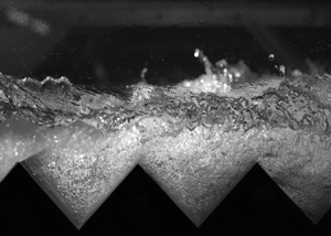
Figure 1. Characteristic regions and modelling approaches of self-aerated open-channel flows: (a) snapshot of the self-aerated flow down a stepped chute (The University of Queensland) with clear distinction of the bubbly flow region and the wavy free-surface region; specific water discharge  $q = 0.143$ m $^2$ s $^{-1}$, chute angle $\theta = 45^\circ$; step edges 5 to 7; (b) schools of thought in the modelling of air concentration distributions in self-aerated flows.
The first group of researchers conceptualized the air concentration distribution using a single-layer approach, thus assuming a ‘homogeneous’ mixing process between the channel bottom and  $y_{90}$, except Valero & Bung (Reference Valero and Bung2016), who described air concentrations within a turbulent–wavy region. Here, $y_{90}$ is the flow depth where the time-averaged air concentration is $\bar {c} = 0.9$, with $\bar {c}$ being defined as volume of air per volume of air–water mixture. Rao & Gangadharaiah (Reference Rao and Gangadharaiah1971) and Wood (Reference Wood1984) derived expressions for the air concentration distribution based on mass conservation considerations, while Chanson (Reference Chanson1995), Chanson & Toombes (Reference Chanson and Toombes2001) and Zhang & Chanson (Reference Zhang and Chanson2017) presented solutions of the advection–diffusion equation for air in water under the assumption of variable turbulent diffusivity across the water depth (up to $y_{90}$). We argue that the assumption of a ‘homogeneous’ bubbly air–water mixture does not contemplate the real structure of a self-aerated flow, as depicted in figure 1(a), although we acknowledge that single-layer approaches can show a good data-driven agreement with typical S-shaped concentration profiles, which is, however, at the expense of empirically fitted coefficients.
Based on flow visualization, Killen (Reference Killen1968) discerned several distinct flow regions of a self-aerated flow (figure 1a), comprising:
(i) a single-phase (water) region next to the channel bottom (not always present);
(ii) a bubbly flow region;
(iii) a free-surface region, characterized by free-surface perturbations/waves; and
(iv) a spray/droplet region.
Wilhelms & Gulliver (Reference Wilhelms and Gulliver2005) identified that measured air concentrations typically comprise entrained air in the form of bubbles and entrapped air between surface roughness/waves, corresponding to regions (ii) and (iii), while very fine droplets, forming region (iv), have only been observed at prototype scale and in near-full-scale facilities (see Table 1 of Hohermuth, Felder & Boes Reference Hohermuth, Felder and Boes2021a; Bai, Tang & Wang Reference Bai, Tang and Wang2022). Further, it is known that the single-phase region (i) vanishes for depth-averaged (mean) air concentrations  $\langle \bar {c} \rangle \gtrapprox 0.25$, which is because the bubbly flow layer protrudes to the channel bottom (Straub & Anderson Reference Straub and Anderson1958; Hager Reference Hager1991; Wei et al. Reference Wei, Xu, Deng and Guo2022). Here, the mean air concentration is defined as
 \begin{equation} \langle \bar{c} \rangle = \frac{1}{y_{90}} \int_{y = 0}^{y_{90}} \bar{c} \, \text{d}y, \end{equation}
where  $y$ is the bed-normal coordinate with $y$ = 0 at the channel invert.
The second group of researchers differentiated between the aforementioned regions using multi-layer approaches, mostly in the form of double-layer models (figure 1b), such as those from Straub & Anderson (Reference Straub and Anderson1958) and Killen (Reference Killen1968), consisting of a lower layer where air bubbles are transported by turbulence throughout the flow, and an upper layer with a heterogeneous mixture of water droplets ejected from the flowing stream. The transition point between the two regions, defined by the depth  $y_\star$ with corresponding air concentration $\bar {c}_\star$, was determined based on the maximum gradient $(\text {d}\bar {c}/\text {d}y)_{max}$ by Straub & Anderson (Reference Straub and Anderson1958). In contrast, Wei & Deng (Reference Wei and Deng2022) argued that the flow depth $y_{50}$, i.e. the depth where $\bar {c} = 0.5$, can be used as interior transition depth, and Wei et al. (Reference Wei, Xu, Deng and Guo2022) proposed some additive concepts to model the air concentration distribution. Generally, a double-layer (or multi-layer) approach better reflects the physical nature of an air–water flow, but an in-depth understanding of the flow transition is currently missing. Furthermore, none of the double-layer models have established a link between the air concentration and the velocity distribution, i.e. a coupling of mass and momentum transfer.
Here, we propose a novel double-layer conceptualization of the air transport, which builds on two canonical flow layers of momentum, namely a turbulent boundary layer (TBL) and a turbulent wavy layer (TWL). We note that the TBL and the TWL conceptually feature a log-law and a constant free-stream velocity distribution, respectively. The air concentration of these layers is modelled using a modified Rouse profile (TBL, corresponds to regions i and ii) and a Gaussian error function (TWL, corresponds to region iii); both layers are convoluted using a two-state principle, which is detailed in § 2. Through analysis of concentration profiles from the literature, we show that the transition between TBL and TWL is closely linked to the boundary layer thickness ( $\delta$), and that other model parameters, such as the Rouse number (Rouse Reference Rouse1961; Dey Reference Dey2014), are unequivocally determined by the mean air concentration (§ 3). For $\langle \bar {c} \rangle \lessapprox 0.25$, the Gaussian error function alone is able to predict the measured air concentration distributions, which suggests that entrapped air (within wave troughs) is prevalent in those flows. In § 4, we quantify the turbulent Schmidt number for aerated flows, followed by a discussion on model limitations.
2. Methodology: two-state air concentration distribution
The general principle of decomposing the streamwise velocity profile (and other flow statistics) into a pure wall flow state and a free-stream state was first introduced by Krug, Philip & Marusic (Reference Krug, Philip and Marusic2017). Here, we hypothesize that the two-state concept can be extended to describe turbulent mass transport, such as the air concentration distribution in supercritical open-channel flows (figure 2). In the following, we seek expressions for the air concentration distribution within the TBL and the TWL.

Figure 2. Two-state model for air concentration distribution: (a) representation of the TBL air concentration (teal line, (2.1)), TWL air concentration (blue line, (2.2)), interface position  $y_i$ and two-state model $\hat {c}$; (b) probability distribution of interface position, centred around $y_\star$; (c) comparison of the convoluted profile (convolution operation indicated by the $\boldsymbol {*}$ symbol) with data from Straub & Anderson (Reference Straub and Anderson1958, specific discharge $q=0.322$ m $^2$ s $^{-1}$; streamwise position $x = 13.88$ m).
2.1. Air concentration within the TBL
We note that the TBL features a log-law velocity distribution and turbulent air bubble diffusion. Assuming a parabolic distribution of turbulent diffusivity ( $D_{t,y}$) up to half the boundary layer thickness, as well as a constant turbulent diffusivity for $y > \delta /2$ (also known as parabolic-constant diffusivity distribution), we obtain a modified Rouse equation by solving the advection–diffusion equation for air in water. The expression for the air concentration $\bar {c}_{TBL}$ within the TBL reads (Appendix A, figure 2a)
 \begin{equation} \bar{c}_{TBL} =\begin{cases} \bar{c}_{\delta/2} \left({\dfrac{y}{\delta-y}} \right)^{\beta}, & y \leq \delta/2,\\ \bar{c}_{\delta/2} \exp \left(\dfrac{4\beta}{\delta} \left(y - \dfrac{\delta}{2} \right) \right), & y > \delta/2, \end{cases} \end{equation}
where  $\bar {c}_{\delta /2}$ is the air concentration at half the boundary layer thickness, $\bar {v}_r$ is the bed-normal bubble rise velocity, $\kappa$ is the von Kármán constant, $u_*$ is the friction velocity and $\beta = \bar {v}_r S_c /\kappa u_*$ is a modified Rouse number, which encapsulates the turbulent Schmidt number $S_c$, the latter defined as the ratio of eddy viscosity and turbulent mass diffusivity. Here, we adopt the classical definition of the boundary layer thickness as the bed-normal distance at which 99 % of the free-stream velocity is attained, as well as a constant value of $\kappa = 0.41$, while we acknowledge that slightly different values of the von Kármán constant have been discussed (Marusic et al. Reference Marusic, McKeon, Monkewitz, Nagib, Smits and Sreenivasan2008; Nagib & Chauhan Reference Nagib and Chauhan2008; Morrill-Winter, Philip & Klewicki Reference Morrill-Winter, Philip and Klewicki2017).
2.2. Air concentration within the TWL
We emphasize that the air concentration of the TWL comprises surface waves/ perturbations (entrapped air) as well as some entrained air bubbles. An analytical solution for the air concentration  $\bar {c}_{TWL}$ involves the Gaussian error function (Valero & Bung Reference Valero and Bung2016); (figure 2a)
 \begin{equation} \bar{c}_{TWL} = \frac{1}{2} \left( 1 + {\rm erf} \left( \frac{y - y_{50_{TWL}}}{ \sqrt{2} \mathcal{H} } \right) \right), \end{equation}
where  $y_{50_{TWL}}$ is the mixture flow depth where the free-surface air concentration is $\bar {c}_{TWL} = 0.5$, $\mathcal {H}$ is a characteristic length scale that describes the thickness/height of the aerated wavy layer and ${\rm erf}$ is the Gaussian error function. In single-phase flows, $\mathcal {H}$ is defined as the root mean square wave height (Valero & Bung Reference Valero and Bung2016). The air concentration of the TWL results from a superposition of entrapped air, transported between wave crests and troughs, and entrained air in the form of air bubbles travelling within the waves (Killen Reference Killen1968; Wilhelms & Gulliver Reference Wilhelms and Gulliver2005). Because the volume of entrapped air within the TWL is typically much larger than the volume of entrained air, $\mathcal {H}$ still provides a clear indication of the root mean square wave height. However, for the sake of accuracy, we hereafter refer to $\mathcal {H}$ as the length scale of the TWL.
2.3. Two-state convolution
Consistent with the two-state formulation of Krug et al. (Reference Krug, Philip and Marusic2017), we introduce the concept of an interface position  $y_i$ separating the TBL and TWL. The air concentration profile $\hat {c}$ is defined for every position of $y_i$
$y_i$
 \begin{equation} \hat{c} =\begin{cases} \bar{c}_{TBL} \ (2.1), & y \leq y_i,\\ \bar{c}_{TWL} \ (2.2), & y > y_i.\\ \end{cases} \end{equation}
Using the Heaviside step function
 \begin{equation} H(y-y_i) =\begin{cases} 0, & y - y_i \leq 0,\\ 1, & y - y_i > 0 ,\\ \end{cases} \end{equation}
we can write (2.3) as
 \begin{equation} \hat{c} = \bar{c}_{TBL} (1-H) + \bar{c}_{TWL}H. \end{equation}
 Equations (2.3) and (2.5) correspond to the discontinuous profile shown in figure 2(a), i.e. the two-state model. It is implied that the flow below the interface level  $y_i$ is fully explained by turbulent air bubble diffusion, whereas turbulent waves describe the air concentration above $y_i$. The interface position is now assumed to follow a random independent process, which is governed by a Gaussian probability distribution shown in figure 2(b)
 \begin{equation} p(y_i; y_\star, \sigma_\star) = \frac{1}{\sigma_\star \sqrt{2{\rm \pi}}} \exp \left( \frac{-(y_i - y_\star)^2}{2\sigma_\star^2} \right), \end{equation}
where the transition depth  $y_\star$ can be interpreted as the time-averaged $y$-location of the interface, and $\sigma _\star$ describes the standard deviation of $y_i$. To obtain a complete, time-averaged expression for the double-layer air concentration (figure 2c), we convolute $\hat {c}$ (2.5) with the interface probability $p$ (2.6), which leads to (Krug et al. Reference Krug, Philip and Marusic2017)
 \begin{equation} \bar{c}(y) = \int_{-\infty}^{\infty} \hat{c} p \, \text{d}y_i = \bar{c}_{TBL} \int_{-\infty}^{\infty} (1-H) p \, \text{d}y_i + \bar{c}_{TWL} \int_{-\infty}^{\infty} H p \, \text{d}y_i, \end{equation}
where  $\bar {c}_{TBL}$ and $\bar {c}_{TWL}$ are independent of $y_i$, thus allowing us to simplify
 \begin{equation} \bar{c}(y) = \bar{c}_{TBL}(1-\varGamma) + \bar{c}_{TWL} \varGamma, \end{equation}
with
 \begin{equation} \varGamma(y; y_\star, \sigma_\star) = \frac{1}{2} \left( 1+{\rm erf} \left(\frac{y - y_\star }{ \sqrt{2} \sigma_\star} \right) \right). \end{equation}
 We note that the lower limit of the integral in (2.7) was extended to  $- \infty$, which, however, did not affect the results as $p(y_i< 0) \ll 1$. From a physical point of view, the convolution can be interpreted as a weighted-averaging operation, which lumps concentration discontinuities between the TBL and TWL, such as the jump shown in figure 2(a), into a smooth, continuous profile. Finally, the interface distribution of the two-state model is not expected to be the same as the turbulent/non-turbulent interface in TBLs; see discussion in Krug et al. (Reference Krug, Philip and Marusic2017).
2.4. Determination of model parameters
The convoluted two-state air concentration model (2.8) has four free physical parameters, including the Rouse number ( $\beta$), the length scale of the TWL ( $\mathcal {H}$) and two transition/interface parameters ( $y_\star$, $\sigma _\star$). We note that the parameters $\delta$, $\bar {c}_{\delta /2}$ and $y_{50_{TWL}}$ are regarded as fixed, as they are directly available from measurements. The free model parameters were derived through a two-step fitting procedure to an extensive experimental data set of air concentration profiles. It is noted that both layers (TBL and TWL) allowed for an independent (simultaneous) fit away from the mean interface position $y_\star$, thus preserving the physical significance of their parameters.
In a first step, the Rouse number  $\beta$ was obtained by minimizing the sum of squared differences between measurements up to $\delta /2$ and (2.1). Here, the boundary layer thickness was computed from measured velocities; if such velocity measurements were not available, we assumed $\delta = 1.25 \, y_\star$ (see § 3.2). At the same time, the length scale $\mathcal {H}$ was obtained by minimizing the sum of squared differences between the measurements and modelled air concentrations within the upper flow region. We note that $y_{50_{TWL}}$ corresponds to $y_{50}$, which is a physical quantity that can be directly measured. However, this was not the case for 46 out of 571 re-analysed profiles with $\langle \bar {c} \rangle \gtrapprox 0.5$, where $y_{50_{TWL}}$ was also obtained through fitting; in this case, the number of free parameters increased by one. In a second step, the mean interface position $y_\star$ was determined at the location where (2.2) departed from the measured air concentrations, which yielded better results when compared with using the maximum gradient $(\text {d}\bar {c}/\text {d}y)_{max}$. Subsequently, the standard deviation $\sigma _\star$ of the interface position was determined using a best-fit approach.
3. Results
We apply our air concentration model to 571 concentration profiles from different data sets, as presented in the supplementary material (available at https://doi.org/10.1017/jfm.2023.440), comprising smooth chute data from Straub & Anderson (Reference Straub and Anderson1958, 74 profiles), Killen (Reference Killen1968, 17 profiles), Bung (Reference Bung2009, 28 profiles) and Severi (Reference Severi2018, 261 profiles), and stepped chute data from Bung (Reference Bung2009, 151 profiles), Zhang (Reference Zhang2017, 6 profiles) and Kramer & Chanson (Reference Kramer and Chanson2018, 34 profiles). The terms ‘smooth’ and ‘stepped’ chute are commonly used in accordance with different roughness heights ( $k_s$) of chute inverts, see figure 1 for an example of a stepped macro-roughness. The category ‘smooth’ also comprises micro-rough inverts, and laboratory spillways are often considered as micro-rough for $k_s \gtrapprox 0.1$ mm (Felder, Severi & Kramer Reference Felder, Severi and Kramer2022). We note that this description slightly differs from the classic smooth/rough classification of wall flows (Pope Reference Pope2000, chap. 7).
3.1. Representative application
We demonstrate the application of our theory using a seminal series of measurements by Straub & Anderson (Reference Straub and Anderson1958), who sampled air concentrations in the uniform region of a smooth chute ( $k_s = 6.1$ mm) for chute angles from $\theta = 7.5^\circ$ to $75^\circ$, covering a wide range of flow rates from $q = 0.13$ to 0.92 m $^2$ s $^{-1}$. These measurements remain among the most comprehensive and complete data sets to date, allowing us to illustrate the relative importance of each of the two states considered.
Figure 3 shows measured air concentrations from Straub & Anderson (Reference Straub and Anderson1958) for  $q = 0.322$ m $^2$ s $^{-1}$, together with the theoretical air concentration profiles of the TBL, TWL and their convolution through the two-state model. For mean air concentrations $\langle \bar {c} \rangle \lessapprox 0.25$ (figure 3a), entrained air bubbles did not reach the channel bottom and aeration was mostly confined to the TWL. Such flows are dominated by entrapped air (free-surface perturbations and turbulent waves), and the air concentration was well described by (2.2); see discussion in Felder et al. (Reference Felder, Severi and Kramer2022). For larger $\langle \bar {c} \rangle$ (figure 3b–h), the air concentration of the TWL (indicated by the blue line) deviated from the measurements at the transition point. Here, the two-state model (2.8) excellently detailed the air concentration measurements, and the corresponding model parameters are presented in table 1.

Figure 3. Measured air concentration distributions in flows down a laboratory smooth chute; data from Straub & Anderson (Reference Straub and Anderson1958,  $q = 0.322$ m $^2$ s $^{-1}$; $x = 13.88$ m); (a–h) comparison of (2.1), (2.2) and (2.8) with measurements.
Table 1. Normalized parameters of the two-state convolution model for profiles shown in figure 3; as no detailed velocity measurements were available from Straub & Anderson (Reference Straub and Anderson1958), we determined  $y_\star$ first, and subsequently assumed $\delta = 1.25 y_\star$ (see § 3.2); measurements taken at $x = 13.88$ m from the flume inlet.

3.2. Profile transition
Next, we focus our attention on the flow transition between TBL and TWL. Figure 4(a,b) shows a measured air concentration profile within the flow centreline of a stepped chute, together with the corresponding streamwise interfacial velocities ( $\bar {u}$) and fluctuations from Kramer & Chanson (Reference Kramer and Chanson2018). Here, $u'_{rms}$ is the root mean square of velocity fluctuations and $\bar {u}_{max}$ is the free-stream velocity. The chute angle was $\theta = 45^\circ$ and measurements were taken at step edge 11, at a specific flow rate of $q = 0.067$ m $^2$ s $^{-1}$. The transition depth $y_\star$ (or mean interface position) was determined through the procedure described in § 2.4 and is shown in figure 4(a).

Figure 4. Determination of the transition point parameters  $y_\star$ and $c_\star$: (a) exemplary air concentration profile, measured within the flow down a stepped spillway; $\theta = 45^\circ$; $q = 0.067$ m $^2$ s $^{-1}$; step edge 11; (b) corresponding normalized velocity profile and velocity fluctuations in the bed-normal direction; (c) ratio of $y_\star$ and boundary layer thickness $\delta$; and (d) air concentration at transition point vs mean air concentration.
A comparison of figure 4(a,b) confirms that the layer below  $y_\star$ (i.e. mainly TBL) was characterized by high flow shearing, whereas the layer above $y_\star$ (TWL) corresponds to a uniform free-stream velocity and, in this instance, the ratio between the transition depth and the boundary layer thickness is $y_\star /\delta = 0.83$. This finding supports our hypothesis that the air concentration distribution is intrinsically connected to the flow momentum layers, both separated by a fluctuating TBL–TWL interface. We find that $y_\star / \delta$ ranges between 0.6 and 0.9 (figure 4c), which is consistent with interface positions reported in Krug et al. (Reference Krug, Philip and Marusic2017). The dimensionless standard deviation of the interface position remains constant at $\sigma _\star /\delta = 0.1$ to 0.2, which yields a good description of all concentration profiles. Our expression for $\sigma _\star$ assumes that the interface position $y_i$ is linked to the underlying TBL edge, while we consider that the waves/perturbations of the TWL – described via $\mathcal {H}$ – are a reflection of that turbulent process. Figure 4(d) shows that the air concentration at the transition point is linearly dependent on the mean air concentration, and can be estimated through the empirical relationship $\bar {c}_\star = 1.37 \langle \bar {c} \rangle - 0.14$, valid for smooth and stepped chutes.
Finally, we acknowledge the scatter in figure 4(c), which likely stems from measurement uncertainties of dual-tip phase-detection probes related to air concentration and interfacial velocity (Kramer et al. Reference Kramer, Hohermuth, Valero and Felder2020; Hohermuth et al. Reference Hohermuth, Kramer, Felder and Valero2021b). We also note that the smooth chute data of Straub & Anderson (Reference Straub and Anderson1958), Killen (Reference Killen1968) and Severi (Reference Severi2018) were not added to figure 4(c), which is because no velocity information was available or because flows were dominated by entrapped air, implying that no profile transition occurred.
3.3. Model parameters related to  $\bar{c}_{TBL}$ and $\bar {c}_{TWL}$


Here, we present estimations of the model parameters related to the air concentration within the TBL and the TWL. An inspection of (2.1) shows that  $\bar {c}_{TBL} = f(\beta, \delta, \bar {c}_{\delta /2})$, of which $\delta$ and $\bar {c}_{\delta /2}$ were directly determined from velocity and air concentration measurements, respectively. The Rouse number $\beta$ reflects the ratio of bubble rise velocity and the strength of turbulence (shear velocity) acting on the entrained air bubbles, and consequently defines the mode of entrained air transport. For example, a small Rouse number implies dominant turbulent forces, which thereof results in a large quantity of small air bubbles being transported close to the channel bed, whereas a large Rouse number implies that large air bubbles are being transported next to the free surface. We find that the described transport modes are dependent on the mean air concentration and that the $\beta$-parameters for stepped chutes were slightly larger than those for smooth chutes (figure 5a), which could be associated with the entrainment of larger air bubbles.

Figure 5. Model parameters are a function of the mean air concentration: (a) Rouse number  $\beta$; (b) relation of TWL mixture flow depth $y_{50_{TWL}}$ to $y_{90}$; (c) relation of TWL length scale $\mathcal {H}$ to $y_{90}$.
The air concentration of the TWL is described by two parameters  $\bar {c}_{TWL} = f(y_{50_{TWL}}, \mathcal {H})$, compare (2.2), of which the mixture flow depth $y_{50_{TWL}}$ was extracted directly from measurements for most of the data sets. Here, we normalize $y_{50_{TWL}}$ and the length scale $\mathcal {H}$ with $y_{90}$, showing their functional dependence on the mean air concentration (figure 5b,c). We note that the normalization with $y_{90}$ provided the most clear relationship, which may simply be because $\langle \bar {c} \rangle$ is defined in terms of $y_{90}$ (1.1). Further, the unique dependence between model parameters and mean air concentration is not completely unexpected, as previous researchers have fitted empirical parameters that only depend on $\langle \bar {c} \rangle$, see for example Chanson (Reference Chanson1995) and Chanson & Toombes (Reference Chanson and Toombes2001). However, it is remarkable that model parameters of the TWL are similarly well behaved for smooth and stepped chutes, and data scatter is only observed beyond $\langle \bar {c} \rangle \gtrapprox 0.5$ to $0.6$. For stepped chutes, the deviation from the linear trend is likely to result from a change in flow regime, i.e. the flow changes from skimming flow to transition flow (Kramer & Chanson Reference Kramer and Chanson2018).
4. Discussion
4.1. Turbulent Schmidt number
In § 3.3, we have discussed the dependence of the depth-averaged parameter  $\beta$ on the mean air concentration. From a Reynolds-averaged modelling perspective, quantifying the turbulent Schmidt number is of interest since it enables a direct relationship between turbulent momentum diffusivity and turbulent mass diffusivity (Pope Reference Pope2000; Gualtieri et al. Reference Gualtieri, Angeloudis, Bombardelli, Jha and Stoesser2017). Hence, we adopt a Reynolds-averaged form of the advection–diffusion equation for air in water (see also Appendix A, (A3))
 \begin{equation} \bar{v}_r \bar{c} = D_{t,y} \frac{\partial \bar{c}}{\partial y}, \end{equation}
which can be conveniently re-arranged
 \begin{equation} D_{t,y} = \frac{\bar{v}_r \bar{c}}{\partial \bar{c} / \partial y}. \end{equation}
 Equation (4.2) allows for a direct evaluation of  $D_{t,y}$ from measurements, given that the local air concentrations, their gradients and the bubble rise velocities are known. For selected profiles from Severi (Reference Severi2018), Kramer & Chanson (Reference Kramer and Chanson2018) and Felder, Hohermuth & Boes (Reference Felder, Hohermuth and Boes2019), we evaluate $\partial \bar {c}/\partial y$ using a central differences approach, and we characterize bubble sizes from intrusive phase-detection probe measurements by adopting the Sauter diameter $d = 6 \bar {c}/a = 1.5 \bar {u} \bar {c}/F$ (Ishii & Hibiki Reference Ishii and Hibiki2011; Hohermuth et al. Reference Hohermuth, Kramer, Felder and Valero2021b), where $a = 4F/\bar {u}$ is the interfacial area per volume of air water mixture (Cummings Reference Cummings1996, equation 4.6.13), and $F$ is the particle count rate. We estimate still water rise velocities ( $\bar {v}_0$) for bubbles with $1\ {\rm mm} < d < 10\ {\rm mm}$ using the approach of Clift, Grace & Weber (Reference Clift, Grace and Weber1978, equation 7-3), which we correct for gravity slope and concentration effects after Chanson (Reference Chanson1995, Reference Chanson1996) as $\bar {v}_r = \bar {v}_0 \cos (\theta ) \sqrt {1-\bar {c}}$. In a next step, we compute turbulent diffusivities through (4.2), which are compared against the boundary layer thickness in figure 6.

Figure 6. Measured turbulent diffusivities vs theoretical parabolic distribution for different turbulent Schmidt numbers.
We consider the classical parabolic turbulent diffusivity distribution (A5) for different  $S_c$-values, which allows us to conclude that the turbulent Schmidt number for air water flows ranges between 0.2 and 1.0 (compare figure 6), which is well in accordance with the published literature values for turbulent mass transfer in other environmental flows (Gualtieri et al. Reference Gualtieri, Angeloudis, Bombardelli, Jha and Stoesser2017). Lastly, the re-analysed smooth chute data suggest that the turbulent diffusivity becomes constant for $y > \delta /2$ (red dotted line), similar to other open-channel flows (Coleman Reference Coleman1970; Dey Reference Dey2014). Based on this finding and reasons outlined in Appendix A, we had already adopted a parabolic-constant diffusivity distribution, splitting the expression for the air concentration within the TBL into two parts, separated by $\delta /2$ (see (2.1)).
4.2. Comparison with other models and limitations
The determination of the four (five) free physical parameters of the convoluted two-state air concentration profile was outlined in § 2.4. Naturally, the number of free parameters is larger than for commonly used single-layer models, e.g. Chanson & Toombes (Reference Chanson and Toombes2001, equation 4.1, two free parameters), and comparable to other double-layer models, e.g. Straub & Anderson (Reference Straub and Anderson1958, four free parameters). However, the introduced parameters respond to physical properties of the flow, and they allow us to assess the relative contribution of individual physical momentum processes on the air concentration profile.
Our theoretical profile ((2.2) for  $\langle \bar {c} \rangle \lessapprox 0.25$ and (2.8) for $\langle \bar {c} \rangle \gtrapprox 0.25$) was able to characterize the air concentration distribution of all tested data sets (see supplementary material), including different flow rates ( $q = 0.03$ to 0.92 m $^2$ s $^{-1}$) and flow regimes over smooth and stepped chutes (transition vs skimming flow), with angles ranging from $\theta = 7.5^\circ$ to $75^\circ$. Model parameters of the TBL and TWL were between $\beta = 0.05$ to $1.2$ (figure 5a) and $\mathcal {H}/y_{90} = 0$ to 1 (figure 5c), both showing a unique dependence on the mean air concentration. The transition/interface parameters were determined as $y_\star /\delta = 0.6$ to 0.9 (figure 4c) and $\sigma _\star /\delta = 0.1$ to 0.2. Given a measured air concentration distribution, $y_\star$ can also be obtained from $\bar {c}_\star$, where the latter followed an empirical relationship $\bar {c}_\star = 1.37 \langle \bar {c} \rangle - 0.14$ (figure 4d).
When compared with previous models, one of the main advantages of the two-state model is its universal applicability, together with physically interpretable model parameters. Previous models rely more heavily on empirical fitting parameters, with application domains being limited to certain chute geometries (smooth vs stepped) or to certain flow regimes (transition vs skimming flow), see for example Chanson & Toombes (Reference Chanson and Toombes2001, Table III-3). Figure 7 compares the convoluted two-state model with common single-layer models for stepped chute data from Bung (Reference Bung2009). All models describe the air concentration reasonably well for  $y/y_{90} \gtrapprox 0.4$, while the models of Wood (Reference Wood1984) and Chanson & Toombes (Reference Chanson and Toombes2001) are upper bounded by $y/y_{90} = 1$. Below $y/y_{90} \lessapprox 0.4$, only the two-state model is able to capture the region which has traditionally been referred to as concentration boundary layer (Chanson Reference Chanson1996), which is due to the novel representation of underlying physical processes.

Figure 7. Comparison of the proposed two-state formulation with common air concentration models for stepped chutes; data from Bung (Reference Bung2009) with  $q = 0.07$ m $^2$ s $^{-1}$; step height $h = 0.06$ m; measurements taken at step edge 16.
The present two-state air concentration model has some limitations, which are herein discussed. The parameters  $\bar {c}_{\delta /2}$ and $\delta$ were directly extracted from original measurements, i.e. no predictive formulas exist, which, however, does not hinder the physical interpretation of mass transport parameters in self-aerated flows. In our derivations related to the modified Rouse profile for air bubbles in water (Appendix A), we have assumed a constant bubble rise velocity as well as uniform flow conditions. To estimate the effect of a concentration-dependent rise velocity, we derive alternative solutions of the advection–diffusion equation using $\bar {v}_r = \bar {v}_0 \cos {(\theta )} \sqrt {1-\bar {c}}$ (Chanson Reference Chanson1995, Reference Chanson1996, Appendix C), where $\bar {v}_0$ is the rise velocity for clear/still water conditions, i.e. $\bar {c} \approx 0$ (similar to § 4.1). Although only marginal differences in resulting concentration profiles were observed (not shown), we cannot rule out that a more detailed assessment of bubble size distributions would help to improve our understanding of the air concentration distribution within the TBL. Related to the uniform equilibrium assumption, our data indicate that (2.1) is also applicable within the gradually varied flow region, which is in agreement with previous findings (Chanson Reference Chanson1995).
5. Conclusion
In this research, we formulate a two-state model to describe air concentration distributions in self-aerated free-surface flows. The rationale behind the model is that the flow can be decomposed into a TBL and a TWL, featuring a log law and a constant free-stream velocity, respectively. The corresponding air concentration distributions are mathematically described by a modified Rouse profile and a Gaussian error function, which conceptually implies that the bubbly flow (within the TBL) is driven by high shear and turbulent diffusion, whereas free-surface waves/perturbations of the TWL lead to large concentrations due to voids within wave troughs.
The transition point between the two layers was previously discussed in the aerated flow literature (Straub & Anderson Reference Straub and Anderson1958), but no physical reasoning was given. Here, we argue that the flow transition corresponds to a time-averaged TBL–TWL interface position that is closely related to the boundary layer thickness. From an instantaneous point of view, the flow takes either a TBL or a TWL state, and the interface position is described by a Gaussian probability density function. Subsequently, a convolution of the two states with the interface probability provides the time-averaged air concentration profile. As such, our model is the first to establish a connection between air concentration and velocity distribution based on physically explainable model parameters.
We test our theoretical air concentration profile against more than 500 experimental concentration profiles from smooth and stepped chute literature data sets. We show that, regardless of the data set, the model is able to capture the profiles and to discern the different air concentration regions contained within. It is noted that laboratory flows with  $\langle \bar {c} \rangle \lessapprox 0.25$ are dominated by free-surface aeration/entrapped air, and the air concentration distribution is confined to the TWL. For larger $\langle \bar {c} \rangle$, air bubbles are diffused deeper into the water column, implying that the time-averaged air concentration is described by the convolution of the Rouse profile and the Gaussian error function with the interface probability. We characterize different transport modes of entrained air bubbles (within the TBL) based on the ratio of bubble rise velocity and shear velocity, expressed through the Rouse number $\beta$, and we show that the transport mode is a function of the mean air concentration. Model parameters related to the TWL were also explained via the mean air concentration and behaved similarly for smooth and stepped chutes. Finally, we present values of the turbulent Schmidt number in highly aerated flows, which we anticipate to be of high relevance for future numerical model applications based on Reynolds-averaged Navier–Stokes equations.
Supplementary material
Supplementary material is available at https://doi.org/10.1017/jfm.2023.440. All data, models or code that support the findings of this study are available from the corresponding author upon reasonable request.
Acknowledgements
We would like to acknowledge fruitful discussions with Dr G. Zhang, AECOM, Australia. We further would like to thank Professor D. Bung (F.H. Aachen), A/Professor S. Felder (UNSW Sydney), Dr B. Hohermuth (ETH Zurich) and Dr A. Severi (Manly Hydraulics Laboratory) for sharing their data sets. At last, we would like to thank the Editor for handling our manuscript, and the anonymous reviewers, whose comments have helped to improve our work.
Funding
This research received no specific grant from any funding agency, commercial or not-for-profit sectors.
Declaration of interests
The authors report no conflict of interest.
Author contributions
Conceptualization, M.K., D.V.; data curation, M.K.; formal analysis, M.K.; methodology, M.K.; investigation, M.K.; visualization, M.K.; software, M.K.; writing – original draft, M.K.; writing – review and editing, M.K., D.V.
Appendix A. Modified Rouse profile for air bubbles in water
A governing equation for the bed-normal air concentration distribution can be written by simplifying the advection–diffusion equation for air in water. We assume a two-dimensional steady flow, where the air concentration only varies in the bed-normal, but not in the streamwise ( $x$) or transverse ( $z$) direction. Therefore, the following gradients can be neglected $\partial ({\cdot })/ \partial t = 0$, $\partial ({\cdot })/ \partial x = 0$, $\partial ({\cdot })/ \partial z = 0$, and the advection–diffusion equation reduces to
 \begin{equation} \frac{\partial (\bar{v}_r \bar{c})}{\partial y} = \frac{\partial }{\partial y} \left( D_{t,y} \frac{\partial \bar{c}}{\partial y} \right), \end{equation}
where  $\bar {v}_r$ is the rise velocity of air bubbles, which is defined positive in bed-normal direction, $\bar {c}$ is the volumetric air concentration (volume of air/total volume) and $D_{t,y}$ is the turbulent diffusivity. We note that the full derivation of the generalized advection–diffusion equation, including Reynolds averaging and gradient diffusion theory, is presented, amongst others, in Dey (Reference Dey2014). A first integration of (A1) leads to
 $$\begin{gather} \int \frac{\partial}{\partial y} (\bar{v}_r \bar{c} ) \,\text{d}y = \int \frac{\partial }{\partial y} \left(D_{t,y} \frac{\partial \bar{c}}{\partial y} \right) \text{d}y, \end{gather}$$
 $$\begin{gather}\bar{v}_r \bar{c} = D_{t,y} \frac{\partial \bar{c}}{\partial y} + \mathcal{K}_1. \end{gather}$$
 To simplify (A3), the partial differential is replaced by the total differential, only the first set of solutions ( $\mathcal {K}_1=0$) is considered and a constant rise velocity is assumed. Separating variables and performing a second integration from an arbitrary elevation $y$ to $\delta /2$ yields
 \begin{equation} \int_{\bar{c}}^{\bar{c}_{{\delta/2}}} \frac{1}{\bar{c}} \, \text{d} \bar{c} = \bar{v}_r \int_{y}^{{\delta/2}} \frac{1}{D_{t,y}} \,\text{d} y. \end{equation}
Now, we invoke a parabolic distribution of turbulent diffusivity (likewise Rouse Reference Rouse1961)
 \begin{equation} D_{t,y} = \frac{\kappa u_* y}{S_c} \left(1 - \frac{y}{\delta}\right), \end{equation}
where  $\kappa$ is the von Kármán constant, $u_*$ is the friction velocity and $S_c$ (= $\nu _t/D_{t,y}$) is the turbulent Schmidt number, defined as the ratio of eddy viscosity $\nu _t$ (i.e. momentum diffusivity) and turbulent mass diffusivity. Substitution and integration of (A4) gives
 \begin{equation} \frac{\bar{c}}{\bar{c}_{{\delta/2}} }= \exp \left( \frac{\bar{v}_r S_c}{\kappa u_*} \ln \left[ \frac{{1}}{\frac{\delta}{y}-1}\right] \right), \end{equation}
which simplifies to
 \begin{equation} \bar{c}(y) = \bar{c}_{{\delta/2}} \left({\frac{y}{\delta-y}} \right)^{\beta}, \quad y \leq \delta/2, \end{equation}
where  $\beta = \bar {v}_r S_c/(\kappa u_* )$ is the Rouse number. It is noted that $S_c$ is assumed constant and (A7) is similar to the well-known Rouse equation for sediment transport but incorporating subtle differences, which are (i) a positively defined bubble rise velocity, (ii) a change of integration limits and (iii) a use of the boundary layer thickness $\delta$ instead of the water depth. The parameter $S_c$ was encapsulated within $\beta$, for convenience.
We note that a purely parabolic diffusivity profile (A5) becomes negative for  $y_i/\delta > 1$, which could occasionally happen if $\sigma _*$ is large. The next appropriate choice is a parabolic-constant diffusivity distribution, which has been used for suspended sediment transport (Coleman Reference Coleman1970; Dey Reference Dey2014), and which we also observe in figure 6, where the turbulent diffusivity $D_{t,y}$ becomes independent of $y$. Adopting a constant $D_{t,y}{(\delta /2)} = \kappa u_* \delta /(4 S_c)$ for $y > \delta /2$, we integrate (A3) between $\delta /2$ and an arbitrary elevation
 \begin{equation} \int_{\bar{c}_{{\delta/2}}}^{\bar{c}} \frac{1}{\bar{c}} \, \text{d} \bar{c} = \bar{v}_r \int_{{\delta/2}}^{y} \frac{4 S_c}{ \kappa u_* \delta} \,\text{d} y, \end{equation}
yielding the following exponential distribution:
 \begin{equation} \bar{c}(y) = \bar{c}_{{\delta/2}} \exp \left(\frac{4 \beta}{\delta} \left(y - {\frac{\delta}{2}} \right) \right), \quad y > \delta/2. \end{equation}


