


1 Introduction
Bedload transport, i.e. the coarser sediment load transported by a flowing fluid in contact with the mobile stream bed by rolling, sliding and/or saltating, has major consequences for public safety, water resources and environmental sustainability. In mountains, steep slopes drive an intense transport of a wide range of grain sizes implying size sorting or segregation (see e.g. Gray Reference Gray2018), which is largely responsible for our limited ability to predict sediment flux and river morphology (Bathurst Reference Bathurst2007; Frey & Church Reference Frey and Church2011; Dudill et al. Reference Dudill, Lafaye de Micheaux, Frey and Church2018). Sediment grain interactions can produce vertical, longitudinal or lateral sorting, which lead to very complex and varied morphologies of bed surface and subsurface (such as armouring, bedload sheet, etc.) (Dietrich et al. Reference Dietrich, Kirchner, Ikeda and Iseya1989; Recking et al. Reference Recking, Frey, Paquier and Belleudy2009; Frey & Church Reference Frey and Church2011; Bacchi et al. Reference Bacchi, Recking, Eckert, Frey, Piton and Naaim2014), and can drastically modify the fluvial geomorphological equilibrium (Dudill, Frey & Church Reference Dudill, Frey and Church2017; Dudill et al. Reference Dudill, Lafaye de Micheaux, Frey and Church2018, Reference Dudill, Venditti, Church and Frey2020).
The present study focuses on vertical size segregation. For large size ratios, the small particles can percolate spontaneously by gravity, without external forcing, into the bed of larger particles (Bridgwater & Ingram Reference Bridgwater and Ingram1971; Dudill et al. Reference Dudill, Frey and Church2017). For the smaller size ratios, spontaneous percolation is not possible without deformation of the bed, which can be achieved by shearing or vibrating. This dynamic segregation results from the combination of kinetic sieving (Middleton Reference Middleton and Lajoie1970) and squeeze expulsion (Savage & Lun Reference Savage and Lun1988). When sheared, the granular material dilates and creates gaps, as the layers of particles flow past one another. Kinetic sieving is based on the idea that, under the action of gravity, small particles are more likely to fall down into the created gaps than the large particles, because they are more likely to fit into the available space. This process competes against squeeze expulsion, which tends to push all particles upwards with the same probability. The combination of both processes, which for brevity will just be called gravity driven segregation (Gray Reference Gray2018), results in a net downward flux of small particles and an upward flux of large grains, leading to an inversely graded bed. Gravity driven segregation has been studied experimentally and numerically in multiple configurations, such as dry granular avalanches (Savage & Lun Reference Savage and Lun1988; Dolgunin & Ukolov Reference Dolgunin and Ukolov1995; Wiederseiner et al. Reference Wiederseiner, Andreini, Epely-Chauvin, Moser, Monnereau, Gray and Ancey2011; Fan et al. Reference Fan, Schlick, Umbanhowar, Ottino and Lueptow2014; Jones et al. Reference Jones, Isner, Xiao, Ottino, Umbanhowar and Lueptow2018), shear cells (Golick & Daniels Reference Golick and Daniels2009; May et al. Reference May, Golick, Phillips, Shearer and Daniels2010; Fan & Hill Reference Fan and Hill2015; Van der Vaart et al. Reference Van der Vaart, Gajjar, Epely-Chauvin, Andreini, Gray and Ancey2015; Fry et al. Reference Fry, Umbanhowar, Ottino and Lueptow2018), annular rotating drums (Gray & Ancey Reference Gray and Ancey2011) and bedload configurations (Ferdowsi et al. Reference Ferdowsi, Ortiz, Houssais and Jerolmack2017; Lafaye de Micheaux, Ducottet & Frey Reference Lafaye de Micheaux, Ducottet and Frey2018; Frey et al. Reference Frey, Lafaye de Micheaux, Bel, Maurin, Rorsman, Martin and Ducottet2020).
Particle-size segregation has strong implications for the study of both geomorphology and granular media in general. It has been studied in many configurations but no general description has been proposed yet. In order to identify the mechanisms and comment on the literature on gravity driven segregation, a dimensional analysis is performed. This analysis is made in the dry limit case, consistent with the results of Maurin, Chauchat & Frey (Reference Maurin, Chauchat and Frey2016) showing that the fluid just acts as a forcing mechanism in turbulent bedload transport and is expected to have only secondary effects on the granular behaviour. Therefore, the fluid is not considered as an influencing parameter for this segregation configuration. The different variables of the problem are
 $$\begin{eqnarray}\begin{array}{@{}cccccccc@{}}d_{s}, & d_{l}, & \unicode[STIX]{x1D70C}_{p}, & g, & \unicode[STIX]{x1D719}_{s}, & \dot{\unicode[STIX]{x1D6FE}}_{p}, & P_{p}, & w_{s},\end{array}\end{eqnarray}$$
 where  $d_{s}$ (respectively $d_{l}$) is the diameter of small (respectively large) particles, $\unicode[STIX]{x1D719}_{s}$ is the local concentration in small particles, $\unicode[STIX]{x1D70C}_{p}$ is the particle density, $g=9.81~\text{ms}^{-2}$ is the gravitational acceleration, $\dot{\unicode[STIX]{x1D6FE}}_{p}$ is the particle shear rate, $P_{p}$ is the granular pressure and $w_{s}$ is the segregation velocity of the small particles. These eight variables involve only three units (length, time and mass), so the problem depends on five dimensionless groups. Choosing $d_{l}$, $\sqrt{d_{l}/g}$ and $\unicode[STIX]{x1D70C}_{p}d_{l}^{3}$ as reference length, time and mass units, respectively, the following relation is obtained:
 $$\begin{eqnarray}{\displaystyle \frac{w_{s}}{\sqrt{gd_{l}}}}={\mathcal{G}}\left(r,\unicode[STIX]{x1D719}_{s},\sqrt{\frac{d_{l}}{g}}\dot{\unicode[STIX]{x1D6FE}}_{p},\frac{P_{p}}{\unicode[STIX]{x1D70C}_{p}d_{l}g}\right),\end{eqnarray}$$
 where  $r=d_{l}/d_{s}$ is the size ratio between large and small particles and ${\mathcal{G}}$ is an unknown function. It is assumed that relation (1.2) can be written in a power law form,
 $$\begin{eqnarray}{\displaystyle \frac{w_{s}}{\sqrt{gd_{l}}}}\propto \left(\sqrt{\frac{d_{l}}{g}}\dot{\unicode[STIX]{x1D6FE}}_{p}\right)^{\unicode[STIX]{x1D701}}\left(\frac{P_{p}}{\unicode[STIX]{x1D70C}_{p}d_{l}g}\right)^{\unicode[STIX]{x1D702}}{\mathcal{G}}_{1}(r){\mathcal{G}}_{2}(\unicode[STIX]{x1D719}_{s}),\end{eqnarray}$$
 where the function  ${\mathcal{G}}_{1}$ should vanish when $r=1$ in order to cancel segregation in the monodisperse limit.
In the theory of Savage & Lun (Reference Savage and Lun1988), the shear rate  $\dot{\unicode[STIX]{x1D6FE}}_{p}$ is predicted to be an important controlling parameter for the rate of particle-size segregation. This is based on the observation that as particles flow downslope, the shear allows each layer of particles in the flow to move faster than the one beneath and hence the rate of finding gaps to fall into is expected to be proportional to the shear rate. Savage & Lun (Reference Savage and Lun1988) showed that this assumption produced good agreement between the theory and bidisperse experimental flows down inclined planes. More recent discrete element method (DEM) simulations of dry bidisperse mixtures in heap flow (Fan et al. Reference Fan, Schlick, Umbanhowar, Ottino and Lueptow2014) have also found there to be a linear relation between the percolation velocity and the shear rate. However, the annular shear cell experiments of Golick & Daniels (Reference Golick and Daniels2009) suggest that the segregation rate is also pressure dependent since the segregation rate dramatically slowed when a large pressure was applied on the top plate of their shear cell. This pressure dependence has also been observed in the DEM simulations of Fry et al. (Reference Fry, Umbanhowar, Ottino and Lueptow2018), who found a power law relating the segregation velocity and the inertial number $I$ (GDR MiDi 2004). A scaling with the inertial number represents an extension of the Savage & Lun (Reference Savage and Lun1988) theory in order to take into account both the effects of the shear rate and pressure on segregation. It corresponds in (1.3) to $\unicode[STIX]{x1D702}=-\unicode[STIX]{x1D701}/2$, which can be rewritten as
 $$\begin{eqnarray}{\displaystyle \frac{w_{s}}{\sqrt{gd_{l}}}}\propto I^{\unicode[STIX]{x1D701}}{\mathcal{G}}_{1}(r){\mathcal{G}}_{2}(\unicode[STIX]{x1D719}_{s}),\end{eqnarray}$$
 with  $I$ the large particle inertial number defined as
 $$\begin{eqnarray}I={\displaystyle \frac{d_{l}\dot{\unicode[STIX]{x1D6FE}}_{p}}{\sqrt{P_{p}/\unicode[STIX]{x1D70C}_{p}}}},\end{eqnarray}$$
suggesting that the segregation velocity is a function of the inertial number, the size ratio and the local concentration.
The size ratio between large and small particles  $r$ is also a key parameter for size segregation. In the annular shear cell, Golick & Daniels (Reference Golick and Daniels2009) showed that the segregation velocity is an increasing function of the size ratio with a maximum around $r=2$. This effect was also observed in both two-dimensional (2-D) and three-dimensional (3-D) DEM simulations of sheared granular flows (Thornton et al. Reference Thornton, Weinhart, Luding and Bokhove2012; Guillard, Forterre & Pouliquen Reference Guillard, Forterre and Pouliquen2016).
The effect of the small particle concentration  $\unicode[STIX]{x1D719}_{s}$ has also been widely studied, and different forms for ${\mathcal{G}}_{2}$ have been proposed (Bridgwater, Foo & Stephens Reference Bridgwater, Foo and Stephens1985; Savage & Lun Reference Savage and Lun1988; Dolgunin & Ukolov Reference Dolgunin and Ukolov1995; Gray & Thornton Reference Gray and Thornton2005; May et al. Reference May, Golick, Phillips, Shearer and Daniels2010; Fan et al. Reference Fan, Schlick, Umbanhowar, Ottino and Lueptow2014; Gajjar & Gray Reference Gajjar and Gray2014; Van der Vaart et al. Reference Van der Vaart, Gajjar, Epely-Chauvin, Andreini, Gray and Ancey2015). The small particles have been shown to segregate less easily if they are more concentrated and the downward velocity should vanish for a pure phase of small particles. For this purpose, the simplest form ${\mathcal{G}}_{2}(\unicode[STIX]{x1D719}_{s})=1-\unicode[STIX]{x1D719}_{s}$, has been proposed by Dolgunin & Ukolov (Reference Dolgunin and Ukolov1995). In oscillating shear cell experiments, Van der Vaart et al. (Reference Van der Vaart, Gajjar, Epely-Chauvin, Andreini, Gray and Ancey2015) measured the time necessary to achieve complete segregation with an initial mixture ranging from one small particle percolating into a bed of large particles, to a single large particle rising up through a small particle bed. They observed that both extreme cases were not symmetric, resulting in an asymmetry of the vertical velocity with the concentration, and Gajjar & Gray (Reference Gajjar and Gray2014) proposed a quadratic dependence of ${\mathcal{G}}_{2}$ on $\unicode[STIX]{x1D719}_{s}$. Fan et al. (Reference Fan, Schlick, Umbanhowar, Ottino and Lueptow2014) and Jones et al. (Reference Jones, Isner, Xiao, Ottino, Umbanhowar and Lueptow2018) also observed this nonlinearity in dry bidisperse avalanche simulations, but concluded that the form of Dolgunin & Ukolov (Reference Dolgunin and Ukolov1995) is a still good first-order approximation.
The literature review on dry granular flows given above underlines the qualitative understanding of size segregation for simple flows. Bedload transport can be seen as a granular flow, where the coupling with the fluid induces strong gradients in the vertical direction and a complex forcing, which could challenge the classical picture of segregation. Few studies have been made on gravity driven segregation in bedload transport and more remains to be done for a clear understanding of the processes at play. Ferdowsi et al. (Reference Ferdowsi, Ortiz, Houssais and Jerolmack2017) experimentally studied size segregation in laminar bedload transport and performed dry granular flow simulations. They studied the formation of armour, i.e. the segregation of large particles to the top, starting from a mixture of small and large particles. They showed that the process seems to be a granular phenomenon and reproduced their experimental results in the framework of continuum segregation modelling, using a generalization of the Gray & Thornton (Reference Gray and Thornton2005) segregation model. Hergault et al. (Reference Hergault, Frey, Métivier, Barat, Ducottet, Böhm and Ancey2010) and Frey et al. (Reference Frey, Lafaye de Micheaux, Bel, Maurin, Rorsman, Martin and Ducottet2020) studied size segregation in turbulent bedload transport, considering a quasi-2-D channel enabling particle tracking. They found that the particles move down as a layer into the bed, and related the segregation velocity to the granular shear rate.
Modelling turbulent bedload transport with segregation phenomenon at the particle scale is computationally demanding and can only be achieved for very small domains. In this context, one of the main goals for segregation in turbulent bedload transport is to be able to do up-scaling to the framework of macroscopic continuum modelling. In this case, it includes the modelling of the fluid phase, the granular phase and the evolution of the different classes of particles with respect to one another. Such a segregation model has been developed by Gray & Thornton (Reference Gray and Thornton2005), Thornton, Gray & Hogg (Reference Thornton, Gray and Hogg2006) and Gray & Chugunov (Reference Gray and Chugunov2006). This three phase model is based on the assumption that the granular overburden pressure is not shared equally between large and small particles (Gray & Thornton Reference Gray and Thornton2005). Substituting this into the momentum conservation equation of each constituent and placing the problem within the framework of the mixture theory, an evolution equation for the phase of small particles is found:
 $$\begin{eqnarray}{\displaystyle \frac{\unicode[STIX]{x2202}\unicode[STIX]{x1D719}_{s}}{\unicode[STIX]{x2202}t}}+\unicode[STIX]{x1D735}\boldsymbol{\cdot }\left(\unicode[STIX]{x1D719}_{s}\boldsymbol{u}\right)-{\displaystyle \frac{\unicode[STIX]{x2202}F_{s}}{\unicode[STIX]{x2202}z}}=\unicode[STIX]{x1D735}\boldsymbol{\cdot }\left(D\unicode[STIX]{x1D735}\unicode[STIX]{x1D719}_{s}\right),\end{eqnarray}$$
 where  $\boldsymbol{u}$ is the bulk velocity field, $F_{s}$ the segregation flux and $D$ the diffusive remixing coefficient of the phase of small particles into the phase of large ones. In this model the fluid has only a passive role and acts through buoyancy to reduce gravity. The physics relies on the expression of the segregation flux and of the diffusion flux. The former is defined as $F_{s}=\unicode[STIX]{x1D719}_{s}w_{s}$ and can therefore directly be linked to the discussion above. Introducing the dimensional analysis (1.4) and considering the simplest form of Dolgunin & Ukolov (Reference Dolgunin and Ukolov1995) for ${\mathcal{G}}_{2}$ the following segregation flux is obtained:
 $$\begin{eqnarray}F_{s}\propto {\mathcal{G}}_{1}(r)I^{\unicode[STIX]{x1D701}}\unicode[STIX]{x1D719}_{s}(1-\unicode[STIX]{x1D719}_{s}).\end{eqnarray}$$
In granular flows, diffusion has been mainly studied in the case of self-diffusion. By analogy to the thermal diffusion of molecules, Campbell (Reference Campbell1997) tracked the random motion of particles in numerical simulations of dilute monodisperse sheared flows, and showed that the diffusion coefficient should scale with the shear rate. In dense 2-D granular Couette flow experiments, Utter & Behringer (Reference Utter and Behringer2004) also observed that the diffusion coefficient was dependent on the shear rate. The diffusion mechanism considered in this paper is the mixing of one class of particles into another. This kind of diffusion is expected to be related to self-diffusion, but to the best of our knowledge, no study has been done in order to determine the physical mechanism controlling this diffusion.
While the literature review above underlines the progress in the understanding and modelling of gravity driven segregation, more physically based parameterizations of the continuum segregation model are still lacking, in particular in the complex turbulent bedload transport configuration. In addition, no general description of size segregation, that would be valid in all configurations, has been proposed yet. From a geomorphological point of view, the impact of size segregation on transport rate is not well understood and an effort is still needed in the development of a model able to represent size segregation at the river scale.
In the present contribution, size segregation in turbulent bedload transport is studied numerically considering fluid-DEM simulations. The aim is to understand size segregation in the quasi-static part of the flow and to improve the continuum modelling parameterizations. In particular, the influence of the three main parameters which are the size ratio  $r$, the inertial number $I$, the small particle concentration $\unicode[STIX]{x1D719}_{s}$, will be investigated through numerical experiments in the bedload configuration.
After presenting the numerical model (§ 2), simulations of turbulent bedload transport will be presented and analysed based on the different expected dependencies from the dimensional analysis (§ 3). The results will then be studied, through a theoretical analysis, in the framework of macroscopic continuum modelling and will highlight the local segregation mechanisms. This analysis shows that diffusion and segregation should have the same dependence on the inertial number and enables quantitatively reproducing the DEM results (§ 4).
2 Fluid-DEM model for bidisperse system
The numerical model used to simulate size segregation in turbulent bedload transport is a three-dimensional DEM using the open-source code YADE (Smilauer et al. Reference Smilauer2015) coupled with a one-dimensional turbulent fluid model. This code has been validated with particle-scale experiments (Frey Reference Frey2014) in Maurin et al. (Reference Maurin, Chauchat, Chareyre and Frey2015) for mono-disperse situations. It was used to study bedload rheology (Maurin et al. Reference Maurin, Chauchat and Frey2016) and the slope influence (Maurin, Chauchat & Frey Reference Maurin, Chauchat and Frey2018). A brief summary of the model formulation as well as a description of its adaptation to bi-disperse situations is now given.
2.1 Granular phase
The DEM is a Lagrangian method based on the resolution of contacts between particles. For each spherical particle  $p$, the motion of the particle is obtained from Newton’s second law, and a momentum equation and an angular momentum conservation equation are solved:
 $$\begin{eqnarray}\displaystyle & \displaystyle m^{p}{\displaystyle \frac{\text{d}^{2}\boldsymbol{x}^{p}}{\text{d}t^{2}}}=\boldsymbol{f}_{g}^{p}+\boldsymbol{f}_{c}^{p}+\boldsymbol{f}_{f}^{p}, & \displaystyle\end{eqnarray}$$
 $$\begin{eqnarray}\displaystyle & \displaystyle {\mathcal{I}}^{p}{\displaystyle \frac{\text{d}\unicode[STIX]{x1D74E}^{p}}{\text{d}t}}=\boldsymbol{{\mathcal{T}}}=\boldsymbol{x}_{c}\times \boldsymbol{f}_{c}^{p}, & \displaystyle\end{eqnarray}$$
 where  $m^{p}$, $\boldsymbol{x}^{p}$, $\unicode[STIX]{x1D74E}^{p}$ and ${\mathcal{I}}^{p}$ are respectively the mass, position, angular velocity and moment of inertia of particle $p$. The three major forces are: $\boldsymbol{f}_{g}^{p}$ the gravitational force, $\boldsymbol{f}_{c}^{p}$ the inter-particle contact forces and $\boldsymbol{f}_{f}^{p}$ the interaction forces with the fluid. The inter-particle contact forces are classically defined as a spring-dashpot system (Schwager & Poschel Reference Schwager and Poschel2007) composed of a spring of stiffness $k_{n}$ in parallel with a viscous damper of coefficient $c_{n}$ in the normal direction; and a spring of stiffness $k_{s}$ associated with a slider of friction coefficient $\unicode[STIX]{x1D707}_{p}$ in the tangential direction. The normal and tangential contact forces read accordingly:
 $$\begin{eqnarray}\left.\begin{array}{@{}c@{}}F_{n}=-k_{n}\unicode[STIX]{x1D6FF}_{n}-c_{n}\dot{\unicode[STIX]{x1D6FF}}_{n},\\ F_{t}=-\text{min}(k_{s}\unicode[STIX]{x1D6FF}_{t},\unicode[STIX]{x1D707}_{p}F_{n}),\end{array}\right\}\end{eqnarray}$$
 where  $\unicode[STIX]{x1D6FF}_{n}$ (respectively $\unicode[STIX]{x1D6FF}_{t}$) is the overlap between particles in the normal (respectively tangential) direction. For each class of particles, the values of $k_{n}$ and $k_{s}$ are computed in order to stay in the rigid limit of grains (Roux & Combe Reference Roux and Combe2002; Maurin et al. Reference Maurin, Chauchat, Chareyre and Frey2015). The normal stiffness, in parallel with the viscous damper, defines a restitution coefficient representative of the loss of energy during collisions, which is fixed to $e_{n}=0.5$ for each contact. Finally, considering glass beads, the friction coefficient is fixed to $\unicode[STIX]{x1D707}_{p}=0.4$ for all particles independently of their diameter.
The third type of forces concern the interactions with the fluid which are restricted in this model to the buoyancy force and the drag force (Maurin et al. Reference Maurin, Chauchat, Chareyre and Frey2015). They are defined as
 $$\begin{eqnarray}\displaystyle & \displaystyle \boldsymbol{f}_{b}^{p}=-{\displaystyle \frac{\unicode[STIX]{x03C0}d^{p3}}{6}}\unicode[STIX]{x1D735}P_{\boldsymbol{x}^{p}}^{\,\,f}, & \displaystyle\end{eqnarray}$$
 $$\begin{eqnarray}\displaystyle & \displaystyle \boldsymbol{f}_{D}^{p}={\displaystyle \frac{1}{2}}\unicode[STIX]{x1D70C}_{f}{\displaystyle \frac{\unicode[STIX]{x03C0}d^{p2}}{4}}C_{D}\Vert \langle \boldsymbol{u}\rangle _{\boldsymbol{x}^{p}}^{f}-\boldsymbol{v}^{p}\Vert \left(\langle \boldsymbol{u}\rangle _{\boldsymbol{x}^{p}}^{f}-\boldsymbol{v}^{p}\right), & \displaystyle\end{eqnarray}$$
 where  $d^{p}$ denotes the diameter of particle $p$,
$p$,  $\langle \boldsymbol{u}\rangle _{\boldsymbol{x}^{p}}^{f}$ is the mean fluid velocity at the position of particle $p$,
$p$,  $P_{\boldsymbol{x}^{p}}^{f}$ is the hydrostatic fluid pressure at the position of particle $p$ and $\boldsymbol{v}^{p}$ is the velocity of particle $p$. The drag coefficient takes into account hindrance effects (Richardson & Zaki Reference Richardson and Zaki1954) as $C_{D}=(0.4+24.4/Re_{p})(1-\unicode[STIX]{x1D6F7})^{-3.1}$, with $\unicode[STIX]{x1D6F7}$ the total solid phase (small and large particle) volume fraction and $Re_{p}=\Vert \langle \boldsymbol{u}\rangle _{\boldsymbol{x}^{p}}^{f}-\boldsymbol{v}^{p}\Vert d^{p}/\unicode[STIX]{x1D708}^{f}$ the particle Reynolds number.
2.2 Fluid model
At transport steady state, the total granular phase (of small and large particles) only has a streamwise component with no main transverse or vertical motion. In such a case, it can be shown (Revil-Baudard & Chauchat Reference Revil-Baudard and Chauchat2013) that the 3-D volume-averaged equation for the fluid velocity reduces to a one-dimensional (1-D) vertical equation, in which the fluid velocity is only a function of the wall-normal component,  $z$, and is aligned with the streamwise direction. The fluid pressure $P^{f}$, is in this case given by the hydrostatic fluid pressure, as shown in Revil-Baudard & Chauchat (Reference Revil-Baudard and Chauchat2013). The proposed fluid model is therefore a one-dimensional turbulent model in the streamwise $x$-direction with variables only depending on $z$ and is inspired from the Euler–Euler model proposed by Revil-Baudard & Chauchat (Reference Revil-Baudard and Chauchat2013) and Chauchat (Reference Chauchat2018). The volume-averaged momentum balance for the fluid phase is as follows:
 $$\begin{eqnarray}\unicode[STIX]{x1D70C}_{f}(1-\unicode[STIX]{x1D6F7}){\displaystyle \frac{\unicode[STIX]{x2202}\langle u_{x}\rangle ^{f}}{\unicode[STIX]{x2202}t}}={\displaystyle \frac{\unicode[STIX]{x2202}S_{xz}}{\unicode[STIX]{x2202}z}}+{\displaystyle \frac{\unicode[STIX]{x2202}R_{xz}}{\unicode[STIX]{x2202}z}}+\unicode[STIX]{x1D70C}_{f}(1-\unicode[STIX]{x1D6F7})g_{x}-n\langle f_{f_{x}}^{p}\rangle ^{s},\end{eqnarray}$$
 where  $\unicode[STIX]{x1D70C}_{f}$ is the density of the fluid, $S_{xz}$ is the effective fluid viscous shear stress of a Newtonian fluid, $R_{xz}$ is the turbulent fluid shear stress and $n\langle f_{f_{x}}^{p}\rangle ^{s}$ represents the momentum transfer associated with the interaction forces between fluid and particles.
The viscous shear stress  $S_{xz}$ is taken as
 $$\begin{eqnarray}S_{xz}=\unicode[STIX]{x1D70C}_{f}(1-\unicode[STIX]{x1D6F7})\unicode[STIX]{x1D708}^{f}{\displaystyle \frac{\unicode[STIX]{x2202}\langle u_{x}\rangle ^{f}}{\unicode[STIX]{x2202}z}},\end{eqnarray}$$
 with  $\unicode[STIX]{x1D708}^{f}$ the pure fluid viscosity. The Reynolds shear stress $R_{xz}$ is based on an eddy viscosity concept,
 $$\begin{eqnarray}R_{xz}=\unicode[STIX]{x1D70C}_{f}(1-\unicode[STIX]{x1D6F7})\unicode[STIX]{x1D708}_{t}{\displaystyle \frac{\unicode[STIX]{x2202}\langle u_{x}\rangle ^{f}}{\unicode[STIX]{x2202}z}}.\end{eqnarray}$$
 The turbulent viscosity  $\unicode[STIX]{x1D708}_{t}$ follows a mixing length approach that depends on the integral of the solid volume fraction profile to account for the presence of particles (Li & Sawamoto Reference Li and Sawamoto1995),
 $$\begin{eqnarray}\unicode[STIX]{x1D708}_{t}=l_{m}^{2}|{\displaystyle \frac{\unicode[STIX]{x2202}\langle u_{x}\rangle ^{f}}{\unicode[STIX]{x2202}z}}|,\quad l_{m}(z)=\unicode[STIX]{x1D705}\displaystyle \int _{0}^{z}{\displaystyle \frac{\unicode[STIX]{x1D6F7}_{max}-\unicode[STIX]{x1D6F7}(\unicode[STIX]{x1D701})}{\unicode[STIX]{x1D6F7}_{max}}}\,\text{d}\unicode[STIX]{x1D701},\end{eqnarray}$$
 with  $\unicode[STIX]{x1D705}=0.41$ the von Kármán constant and $\unicode[STIX]{x1D6F7}_{max}=0.61$ the maximal packing of the granular medium (random close packing).
The total momentum  $n\langle f_{f_{x}}^{p}\rangle ^{s}$ transmitted by the fluid to the particles is computed as the sum over each class of the horizontal solid-phase average (denoted $\langle .\rangle ^{s}$) of the momentum transmitted by the drag force on each particle
 $$\begin{eqnarray}n\langle f_{f_{x}}^{p}\rangle ^{s}={\displaystyle \frac{\unicode[STIX]{x1D6F7}_{s}}{\unicode[STIX]{x03C0}d_{s}^{3}/6}}\langle f_{f_{x}}^{p_{s}}\rangle ^{s}+{\displaystyle \frac{\unicode[STIX]{x1D6F7}_{l}}{\unicode[STIX]{x03C0}d_{l}^{3}/6}}\langle f_{f_{x}}^{p_{l}}\rangle ^{s},\end{eqnarray}$$
and introducing the expression of the drag force (2.5),
 $$\begin{eqnarray}\displaystyle n\langle f_{f_{x}}^{p}\rangle ^{s} & = & \displaystyle {\displaystyle \frac{3}{4}}{\displaystyle \frac{\unicode[STIX]{x1D6F7}_{s}\unicode[STIX]{x1D70C}_{f}}{d_{s}}}\langle C_{D}\Vert \langle \boldsymbol{u}\rangle _{\boldsymbol{x}^{p_{s}}}^{f}-\boldsymbol{v}^{p_{s}}\Vert (\langle \boldsymbol{u}\rangle _{\boldsymbol{x}^{p_{s}}}^{f}-\boldsymbol{v}^{p_{s}})\rangle ^{s}\nonumber\\ \displaystyle & & \displaystyle +\,{\displaystyle \frac{3}{4}}{\displaystyle \frac{\unicode[STIX]{x1D6F7}_{l}\unicode[STIX]{x1D70C}_{f}}{d_{l}}}\langle C_{D}\Vert \langle \boldsymbol{u}\rangle _{\boldsymbol{x}^{p_{l}}}^{f}-\boldsymbol{v}^{p_{l}}\Vert (\langle \boldsymbol{u}\rangle _{\boldsymbol{ x}^{p_{l}}}^{f}-\boldsymbol{v}^{p_{l}})\rangle ^{s},\end{eqnarray}$$
 where  $p_{s}$ (respectively $p_{l}$) denotes the ensemble of the small (respectively large) particles, $\unicode[STIX]{x1D6F7}_{s}$ (respectively $\unicode[STIX]{x1D6F7}_{l}$) the volume fraction of small (respectively large) particles and $d_{s}$ (respectively $d_{l}$) the diameter of small (respectively large) particles.
The solid-phase volume average  $\langle \cdot \rangle ^{s}$ is defined following Jackson (Reference Jackson2000) for which a cuboid weighting function ${\mathcal{F}}$ with the same length and width as the 3-D domain is applied. In the vertical direction, in order to capture the strong vertical gradient of the mean flow, the vertical thickness $l_{z}$ of the box is chosen as $l_{z}=d_{s}/30$. This choice of weighting function has been validated by comparison with mono-disperse turbulent bedload transport experiments in Maurin et al. (Reference Maurin, Chauchat, Chareyre and Frey2015). Therefore the mean values at position $z$ are computed as
 $$\begin{eqnarray}\displaystyle & \displaystyle \unicode[STIX]{x1D6F7}_{s}(z)=\mathop{\sum }_{p_{s}}\int _{V_{p_{s}}}{\mathcal{F}}(|z-z^{\prime }|)\,\text{d}z^{\prime }, & \displaystyle\end{eqnarray}$$
 $$\begin{eqnarray}\displaystyle & \displaystyle \unicode[STIX]{x1D6F7}_{l}(z)=\mathop{\sum }_{p_{l}}\int _{V_{p_{l}}}{\mathcal{F}}(|z-z^{\prime }|)\,\text{d}z^{\prime }, & \displaystyle\end{eqnarray}$$
 $$\begin{eqnarray}\displaystyle & \displaystyle \langle \unicode[STIX]{x1D6FE}\rangle ^{s}={\displaystyle \frac{1}{\unicode[STIX]{x1D6F7}_{s}(z)}}\mathop{\sum }_{p_{s}}\int _{V_{p_{s}}}\unicode[STIX]{x1D6FE}(z^{\prime }){\mathcal{F}}(|z-z^{\prime }|)\,\text{d}z^{\prime }+{\displaystyle \frac{1}{\unicode[STIX]{x1D6F7}_{l}(z)}}\mathop{\sum }_{p_{l}}\int _{V_{p_{l}}}\unicode[STIX]{x1D6FE}(z^{\prime }){\mathcal{F}}(|z-z^{\prime }|)\,\text{d}z^{\prime }, & \displaystyle \nonumber\\ \displaystyle & & \displaystyle\end{eqnarray}$$
 where  $\unicode[STIX]{x1D6FE}$ is a scalar quantity.
The fluid model, which is classical in sediment transport (e.g. Drake & Calantoni Reference Drake and Calantoni2001; Hsu & Liu Reference Hsu and Liu2004; Durán, Andreotti & Claudin Reference Durán, Andreotti and Claudin2012; Revil-Baudard & Chauchat Reference Revil-Baudard and Chauchat2013; Maurin et al. Reference Maurin, Chauchat, Chareyre and Frey2015; Chauchat Reference Chauchat2018) is only closed using a mixing length model and a closure for the drag force formulation. The latter are usual in the literature, and it has been shown in Maurin (Reference Maurin2015) and Maurin et al. (Reference Maurin, Chauchat, Chareyre and Frey2015) that the results obtained in terms of granular behaviour are very weakly sensitive to the fluid closure adopted. In this paper, the model is used for a bi-disperse situation to study size segregation in bedload sediment transport.
3 DEM simulations of segregation dynamics
In this section, the infiltration of fine particles into the bed made of larger particles is studied during turbulent bedload transport using the numerical model described in the previous section.
3.1 Numerical set-up
The numerical set-up is presented in figure 1. In the following, subscripts  $l$ and $s$ denote quantities for large and small particles, respectively. Initially, large particles of diameter $d_{l}=6$ mm and fine particles of diameter $d_{s}=4$ mm (size ratio $r=1.5$) are deposited by gravity over a rough fixed bed made of large particles. The particle and fluid densities are fixed respectively to $\unicode[STIX]{x1D70C}^{p}=2500~\text{kg}~\text{m}^{-3}$ and $\unicode[STIX]{x1D70C}^{f}=1000~\text{kg}~\text{m}^{-3}$. The size of the 3-D domain is $30d_{l}\times 30d_{l}$ in the horizontal plane in order to have converged average values (Maurin et al. Reference Maurin, Chauchat, Chareyre and Frey2015) and is periodic in the streamwise and spanwise directions. The number of particles of each class is assimilated into a number of layers, $N_{l}$ and $N_{s}$. The number of layers represents in terms of particle diameters the height that would be occupied by the particles if the packing fraction was exactly 0.61. Equivalently, the volume occupied by large particles (respectively small particles) is $0.61\times 30d_{l}\times 30d_{l}\times N_{l}d_{l}$ (respectively $0.61\times 30d_{l}\times 30d_{l}\times N_{s}d_{s}$). Therefore, fixing $N_{l}$ or $N_{s}$ fixes the number of particles of each class. The height of the bed at rest is defined by $H=N_{l}d_{l}+N_{s}d_{s}$ and $H$ is fixed to $10d_{l}$ in all the simulations. The number of layers of fine particles $N_{s}$ varies from $0.01$ (only a few small particles) up to $2$ layers (corresponding to figure 1), while $N_{l}$ changes accordingly in order to keep $H=10d_{l}$. The bed slope is fixed to $10\,\%$ ( $5.7^{\circ }$), representative of mountain streams. The Shields number is defined as the dimensionless fluid bed shear stress $\unicode[STIX]{x1D703}=\unicode[STIX]{x1D70F}_{f}/[(\unicode[STIX]{x1D70C}_{p}-\unicode[STIX]{x1D70C}_{f})gd_{l}]$ and simulations are performed at $\unicode[STIX]{x1D703}\simeq 0.1$. For this purpose, the free surface position is fixed and corresponds to a water depth of $h=3.1d_{l}$.
At the beginning of each simulation, the fluid flows by gravity and sets particles into motion. A first transient phase takes place, during which fluid and particles are accelerating. During this period, segregation is very fast and at the end of the transient phase, the small particles have already infiltrated into the first layers of the bed. In this paper, the study focuses on the dynamics of segregation once the system is at transport equilibrium and small particles have reached the quasi-static layer.

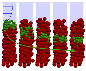
Figure 1. A typical numerical set-up for  $N_{s}=2$. Initially, $N_{s}$ layers of small particles ( $d_{s}=3$ mm) are deposited by gravity above $N_{l}$ layers of large particles ( $d_{l}=6$ mm). $N_{s}$ varies from $0.01$ until $2$ with $N_{l}$ varying accordingly in order to always have $N_{l}d_{l}+N_{s}d_{s}=10d_{l}$.
The horizontal-averaged volume fraction per unit granular volume of small (respectively large) particles is defined as  $\unicode[STIX]{x1D719}_{s}$ (respectively $\unicode[STIX]{x1D719}_{l}$). By definition, the two volume fractions sum to unity,
 $$\begin{eqnarray}\unicode[STIX]{x1D719}_{s}+\unicode[STIX]{x1D719}_{l}={\displaystyle \frac{\unicode[STIX]{x1D6F7}_{s}}{\unicode[STIX]{x1D6F7}_{s}+\unicode[STIX]{x1D6F7}_{l}}}+{\displaystyle \frac{\unicode[STIX]{x1D6F7}_{l}}{\unicode[STIX]{x1D6F7}_{s}+\unicode[STIX]{x1D6F7}_{l}}}=1,\end{eqnarray}$$
 where  $\unicode[STIX]{x1D6F7}_{s}$ (respectively $\unicode[STIX]{x1D6F7}_{l}$) is the volume fraction of small (respectively large) particles defined per unit mixture volume as in the previous section. Lastly, $z_{c}$ is defined as the vertical position of the centre of mass of small particles and $\text{d}z_{c}/\text{d}t$ as its velocity.
The results are presented without dimension and the following dimensionless variables are considered:
 $$\begin{eqnarray}\tilde{z}={\displaystyle \frac{z}{d_{l}}},\quad \tilde{t}=t\sqrt{g/d_{l}},\quad \widetilde{\langle v_{x}\rangle ^{p}}={\displaystyle \frac{\langle v_{x}\rangle ^{p}}{\sqrt{gd_{l}}}}.\end{eqnarray}$$
In the following, the tildes are dropped for sake of clarity.
3.2 Results

Figure 2. (a) Typical temporal evolution of fine particle concentration profile  $\unicode[STIX]{x1D719}_{s}$ for the case $N_{s}=2$, (b) concentration profiles in small particles for different times for the case $N_{s}=2$ and (c) time evolution of the maximal value of $\unicode[STIX]{x1D719}_{s}$ for all simulations.
Simulations have been performed for different numbers of layers of small particles  $N_{s}$. Figure 2(a) shows the temporal evolution of fine particle concentration profiles for the case $N_{s}=2$, corresponding to two layers of small particles deposited on top of a layer made of large particles. At the beginning, the small particles infiltrate rapidly into the first few layers of large particles. As small particles infiltrate downward, large particles rise to the surface. The DEM simulations exhibit a two-layer structure, with small particles sandwiched between two layers of large particles. While infiltrating, the thickness of the small particle layer gets slightly larger. Profiles of concentration for different times are presented in figure 2(b). The concentration profiles exhibit a Gaussian-like shape. After the transient phase, neither the maximal value (see figure 2c) nor the width of the profiles evolve in time, suggesting that the small particles infiltrate the bed as a layer having a constant thickness and that this layer is just convected downward by segregation inside the layer of large particles.

Figure 3. (a) Streamwise space–time-averaged particle velocity as a function of the height, (b) time-averaged volume fraction of the granular mixture and (c) evolution of the vertical position of the mass centre of small particles with time.
The vertical time- and volume-averaged streamwise velocity profile of the particle mixture is plotted in figure 3(a) for all the simulations. All the curves are superimposed meaning that the response of the granular medium to the fluid flow forcing is not modified by the number of small particles. The granular forcing is therefore the same for all the simulations independently of the number of small particles in the initial condition. In the quasi-static region (i.e. between  $z=3$ and $8$ approximately), the linearity of the profiles in the semi-log plot indicates that the velocity is exponentially decreasing in the bed. Due to the presence of a fixed layer of particles at the bottom of the domain, the velocity goes to zero there. It is interesting to note that the entire bed is in motion, even if the velocity can be very low at the bottom of the quasi-static region. This is characteristic of a creeping flow. The time mean solid volume fraction of the mixture is plotted in figure 3(b) for all the simulations. The quasi-static region is characterized by the bed at random close packing ( $\unicode[STIX]{x1D6F7}\sim 0.61$). Above $z\sim 8$, the packing fraction decreases to zero, corresponding to a transition zone between a quasi-static region and a pure fluid phase. Note that due to this decompaction of the bed at the surface, the total height of the bed is slightly larger than $10d_{l}$.
Since the small particles infiltrate the bed as a layer, the centre of mass of the small particles,  $z_{c}$, is a representative position of the entire layer. Figure 3(c) shows the temporal evolution of this position for all the simulations, in a semi-logarithmic plot. After the initial transient phase, the curves become linear, meaning that $z_{c}$ is a logarithmic function of time
 $$\begin{eqnarray}z_{c}=-a\ln (t)+b.\end{eqnarray}$$
 In (3.3), the coefficient  $a$ corresponds to the absolute slope of the curve and characterizes the segregation velocity ( $\text{d}z_{c}/\text{d}t=-a/t$). Whatever the number of small particles in the simulation, figure 3(c) shows that all the curves are parallel to one another, meaning that $a$ is independent of the number of layers of small particles, $N_{s}$. Therefore the segregation velocity $\text{d}z_{c}/\text{d}t$ is also independent of the number of layers of small particles.
In the following, these simulations will be analysed using the dimensional analysis presented in the introduction (1.4) with the aim to confirm the dependence of the segregation flux on the inertial number  $I$ and on the local concentration $\unicode[STIX]{x1D719}_{s}$.
3.3 Dependence on the inertial number
In figure 4(a), the dimensionless segregation velocity is plotted against the large particle inertial number  $I=\dot{\unicode[STIX]{x1D6FE}}_{p}d_{l}/\sqrt{P_{p}/\unicode[STIX]{x1D70C}_{p}}$, where $\dot{\unicode[STIX]{x1D6FE}}_{p}$ is the time mean fluid shear rate and $P_{p}$ is the time mean lithostatic granular pressure. The segregation velocity is higher for larger inertial number. The linearity of the curves shows that the segregation velocity is indeed a power law of the inertial number. For all the simulations a similar exponent is obtained, ranging from $0.81$ to $0.88$, and a best fit gives a value of $0.85$ for the mean exponent,
 $$\begin{eqnarray}{\displaystyle \frac{\text{d}z_{c}(t)}{\text{d}t}}\propto I^{0.85}(z_{c}(t)).\end{eqnarray}$$
 Interestingly, Fry et al. (Reference Fry, Umbanhowar, Ottino and Lueptow2018) obtained a very similar result for dry granular flows at higher inertial numbers ( $I\in [10^{-2},1]$). They obtained an exponent $0.84$, very close to the $0.85$ exponent obtained in the present configuration. Our results suggest that the behaviour observed by Fry et al. (Reference Fry, Umbanhowar, Ottino and Lueptow2018) is valid in a wider range of inertial numbers, in particular, in the quasi-static regime ( $I\in [10^{-5},10^{-1}]$).

Figure 4. (a) Segregation velocity dependence on the local inertial number, (b) inertial number profile.
The scaling with the inertial number (3.4) is in line with the theory of Savage & Lun (Reference Savage and Lun1988) who suggested relating the segregation velocity to the shear rate. Indeed the inertial number is the dimensionless ratio between the shear rate and the square root of pressure. In the bedload configuration, the pressure increases linearly with depth while the shear rate exponentially decreases in the bed. Therefore, most of the variation of the inertial number is contained in the shear rate. A scaling with the inertial number allows the effect of pressure  $P_{p}$ to be taken into account, which is small in this configuration, but the similarity with the results of Fry et al. (Reference Fry, Umbanhowar, Ottino and Lueptow2018) is encouraging in the understanding of size segregation in general.
Equation (3.4) allows the temporal evolution of the fine particles centre of mass to be understood. Figure 4(b) shows the inertial number profile for all simulations. The linearity of the curves, for  $z\leqslant 8$, in the semi-log plot indicates that the inertial number is an exponential function of $z$ in the quasi-static part of the bed. Taking an exponential profile to the power $0.85$, $I^{0.85}$ is also an exponential function of $z$ and can be written as
 $$\begin{eqnarray}I^{0.85}(z)=I_{0}\text{e}^{z/c}.\end{eqnarray}$$
Introducing (3.5) into expression (3.4) leads to
 $$\begin{eqnarray}{\displaystyle \frac{\text{d}z_{c}(t)}{\text{d}t}}=-b_{1}\text{e}^{z_{c}(t)/c},\end{eqnarray}$$
 with  $b_{1}$ a positive constant. Equation (3.6) can be integrated
 $$\begin{eqnarray}\int \text{e}^{-z_{c}/c}\,\text{d}z_{c}=\int -b_{1}\,\text{d}t,\end{eqnarray}$$
leading to
 $$\begin{eqnarray}c\text{e}^{-z_{c}/c}=b_{1}t+\text{Const}\sim b_{1}t,\end{eqnarray}$$
for long times. It can be rewritten as
 $$\begin{eqnarray}z_{c}(t)=-c\ln (t)+b_{2},\end{eqnarray}$$
 where  $b_{2}=-c\ln (b_{1}/c)$ is a constant. This analysis shows that the logarithmic descent of the small particle centre of mass is a consequence of the dependence of the segregation velocity on the inertial number. This is confirmed by the comparison between the coefficients $a$ in (3.3) and $c$ in (3.5), that should be equal. Fitting of the elevation of the centre of mass (figure 3c) and of $I^{0.85}$ yields coefficients $a$ and $c$ (see table 1). The maximal difference between $a$ and $c$ is approximately $3\,\%$ confirming the present analysis and showing that the inertial number is indeed the controlling parameter.
Table 1. Values of coefficients  $a$ (slope of the centre of mass) and $c$ (exponential decay of the inertial number to the power $0.85$) obtained from fitting the curves of figures 3(c) and 4(b) and the error in percentage.


Figure 5. (a) Centre of mass velocity dependence on the inertial number at the bottom of the layer of small particles, (b) small particle concentration profiles at time  $t=40\,435$ and vertical position of the bottom of the layer ( $\times$).
3.4 Bottom controlled segregation
While this analysis clearly explains the trends observed, figure 4(a) shows that for a given value of the inertial number, different segregation velocities are obtained depending on the initial number of small particles,  $N_{s}$.
Since the inertial number follows an exponential profile, it varies importantly throughout the layer of small particles. Thus according to (3.4) the segregation velocity should be lower at the bottom than at the top of the layer. This lower segregation velocity at the bottom of the layer implies that all the small particles above cannot move downward faster than the lowest particles in the layer. Defining the position of the bottom of the layer as  $z_{b}=z_{c}-W/2$, with $W=2N_{s}d_{s}/d_{l}$ the small particle layer thickness, figure 5(a) shows the dependence of the segregation velocity on the inertial number at the bottom of the layer. All the curves collapse on a master curve and a power law relationship is found between the segregation velocity and the inertial number at the bottom of the layer $I_{b}(z_{c})=I(z_{b})$,
 $$\begin{eqnarray}{\displaystyle \frac{\text{d}z_{c}(t)}{\text{d}t}}=-\unicode[STIX]{x1D6FC}_{0}I_{b}^{0.85}(z_{c}(t)),\end{eqnarray}$$
 where  $\unicode[STIX]{x1D6FC}_{0}$ is a positive constant independent of the number of layers of small particles. This result shows that the segregation velocity of the layer is indeed completely controlled by the inertial number at the bottom of the layer and it does not contain any dependence on the number of small particle layers, $N_{s}$.
The layer thickness has been chosen to be two times the thickness it would occupy if only small particles were present,  $W=2N_{s}d_{s}/d_{l}$. This choice is motivated by the fact that the layer is formed of a mixture of both large and small particles. Figure 5(a) shows that, for the different cases, the width obtained is indeed consistent with the actual thickness. Note that when $N_{s}$ tends to zero, $z_{b}$ tends to $z_{c}$ the centre of mass of the small particles. In the extreme case where only one small particle is present, this position corresponds to its centre. Figure 5(b) shows, at time $t=40\,435$, the profiles of small particle concentration, where the crosses denote the position of the bottom of the layer. The lower limbs of the concentration profiles are superimposed and the position of the bottom of the layer is identical for all tested values of $N_{s}$. Whatever the number of small particles, they pile up above the bottom position, where the segregation dynamics is controlled.
It is remarkable that the continuum description (3.10) is applicable even for the cases  $N_{s}=0.01$ and $N_{s}=0.05$, corresponding to very few non-interacting particles and for which a continuum vision seems at first hardly relevant. This can be explained by the bottom controlled dynamics. The isolated particles are placed at the bottom position which is a stable position. Since for cases $N_{s}=0.01$ and $N_{s}=0.05$, $z_{b}$ and $z_{c}$ are located at the same elevation, the continuum description captures the dynamics of isolated particles.
This analysis highlights the dependence of segregation on the inertial number in bedload transport. Furthermore, the bottom of the small particles layer is shown to be a key position that controls segregation. In particular, it explains why the small particles infiltrate the bed as a layer of constant thickness.
3.5 Size ratio influence
The analysis presented above provides a reference position that describes the segregation dynamics. In the following, the effect of the size ratio is investigated. The previous simulations were all performed at the same size ratio,  $r=1.5$. According to the dimensional analysis, the following relationship is expected:
 $$\begin{eqnarray}{\displaystyle \frac{\text{d}z_{c}(t)}{\text{d}t}}=-\unicode[STIX]{x1D6FC}_{0}{\mathcal{G}}_{1}(r)I_{b}^{0.85}(z_{c}(t)).\end{eqnarray}$$
 A set of simulations in which the diameter of the small particles is varied has been performed. It covers a range of size ratios from  $r=1.15$ to $3$. In all these simulations, the number of small particles layer is fixed to $N_{s}=1$. The dependence of the centre of mass velocity on the inertial number at the bottom of the layer of small particles is plotted in figure 6(a). A similar power law relationship is recovered, showing that the inertial number is still the controlling parameter. The best fit provides a $0.82$ exponent, which is in the range of values found previously. However, to remain consistent with the previous analysis an exponent of $0.85$ is used in what follows. The curves are parallel but not superimposed, which implies that, as expected, the size ratio plays an important role in the segregation dynamics. The dependence with the size ratio is presented in figure 6(b) where the ratio between the segregation velocity and the inertial number to the power $0.85$ is plotted as a function of the size ratio minus one. The dependence with the size ratio tends to zero when $r$ is close to unity, cancelling segregation in the monodisperse limit, and increases strongly when the size ratio increases. The following functional form for ${\mathcal{G}}_{1}$ is proposed:
 $$\begin{eqnarray}{\mathcal{G}}_{1}(r)=0.45(\text{e}^{(r-1)/1.59}-1),\end{eqnarray}$$
empirically fitted from the data points of figure 6(b), and plotted in dashed line in figure 6(b).

Figure 6. (a) Centre of mass velocity dependence on the inertial number at the bottom of the layer of small particles for different size ratio. Note that for  $r=2.5$, $r=2.75$ and $r=3$, simulations were performed with a $15d_{l}\times 15d_{l}$ box in order to gain computation time. (b) Best fit coefficient between the segregation velocity and the inertial number to the power $0.85$ times $\unicode[STIX]{x1D6FC}_{0}$ as a function of the size ratio minus one (for each curve of figure 6a, one point is obtained). The function ${\mathcal{G}}_{1}$ is plotted as dashed line.
The maximal efficiency at  $r=2$ reported by Golick & Daniels (Reference Golick and Daniels2009), Thornton et al. (Reference Thornton, Weinhart, Luding and Bokhove2012) and Guillard et al. (Reference Guillard, Forterre and Pouliquen2016) is not recovered in this configuration as the segregation velocity still increases for $r>2$. Further research is necessary to gain better understanding of the size ratio effect on segregation.
To summarize, the results presented here suggest that the segregation dynamics in bedload transport can be described, to leading order, by the following relationship:
 $$\begin{eqnarray}{\displaystyle \frac{\text{d}z_{c}}{\text{d}t}}=-\unicode[STIX]{x1D6FC}_{0}{\mathcal{G}}_{1}(r)I_{b}^{0.85},\end{eqnarray}$$
 where  $\unicode[STIX]{x1D6FC}_{0}$ can be computed from figure 5(a) and ${\mathcal{G}}_{1}(r)$ is given by (3.12).
3.6 Dependence on the local concentration  $\unicode[STIX]{x1D719}_{s}$

It is remarkable that the trends observed for the evolution of the centre of mass and for the segregation velocity are independent of the number of small particle layers,  $N_{s}$. Indeed, as the latter is increased from 0.01 to 2, the configuration moves from a few isolated (non-interacting) small particles to two consistent layers of small particles infiltrating collectively inside the coarse bed. Therefore, it is expected that the increase of $N_{s}$, would increase the local particle concentration and reduce the segregation velocity due to particle hindrance effects.
This independence of the trend observed in the segregation velocity seems in contradiction with the literature (e.g. Savage & Lun Reference Savage and Lun1988; Dolgunin & Ukolov Reference Dolgunin and Ukolov1995; Van der Vaart et al. Reference Van der Vaart, Gajjar, Epely-Chauvin, Andreini, Gray and Ancey2015; Jones et al. Reference Jones, Isner, Xiao, Ottino, Umbanhowar and Lueptow2018), in which a major influence of the local small particle concentration on the segregation velocity has been evidenced. In order to explain this apparent contradiction and get more insight into the physical processes at play, the results are discussed in the following as a function of local mechanisms within the framework of the continuum model of Gray & Thornton (Reference Gray and Thornton2005), Thornton et al. (Reference Thornton, Gray and Hogg2006) and Gray & Chugunov (Reference Gray and Chugunov2006).
4 Discussion in the framework of continuum modelling
4.1 Local mechanism interpretation
In order to explain the apparent independence of the results on the concentration of small particles, a local analysis in the theoretical framework of continuum modelling is considered. The model of Thornton et al. (Reference Thornton, Gray and Hogg2006) (1.6), presented briefly in the introduction, will be used as a baseline. In the present configuration, the velocity field has only a streamwise component (along  $x$) and all quantities only depend on $z$. As a first step, diffusion is not considered and (1.6) simplifies to a purely hyperbolic equation,
 $$\begin{eqnarray}{\displaystyle \frac{\unicode[STIX]{x2202}\unicode[STIX]{x1D719}_{s}}{\unicode[STIX]{x2202}t}}-{\displaystyle \frac{\unicode[STIX]{x2202}F_{s}}{\unicode[STIX]{x2202}z}}=0.\end{eqnarray}$$
Combining the form proposed in the introduction (1.7), the analysis of the DEM simulations (3.13) and the inertial number functional form (3.5), the segregation flux can be written as
 $$\begin{eqnarray}F_{s}=\unicode[STIX]{x1D6FC}_{0}{\mathcal{G}}_{1}(r)I^{0.85}\unicode[STIX]{x1D719}_{s}(1-\unicode[STIX]{x1D719}_{s})=S_{r0}\text{e}^{z/c}\unicode[STIX]{x1D719}_{s}(1-\unicode[STIX]{x1D719}_{s}),\end{eqnarray}$$
 with  $S_{r0}=\unicode[STIX]{x1D6FC}_{0}{\mathcal{G}}_{1}(r)I_{0}$. The inertial number does not depend on the number of small particles (figure 4b) so $S_{r0}$ is independent on the initial number of small particles and only depends on the response of the granular mixture to the fluid flow forcing through $I_{0}$ and $c$. For $r=1.5$, the corresponding value of $S_{r0}$ obtained from the DEM simulations is: $S_{r0}=3.70\times 10^{-8}$. Due to the exponential decrease of the inertial number in the bed, the form of the segregation flux, $F_{s}$, is also exponential with $z$. May et al. (Reference May, Golick, Phillips, Shearer and Daniels2010) already proposed an analytical solution for an exponential flux, but the flow was shear driven from the bottom. Proceeding similarly, the analytical solution can be derived using the method of characteristics (appendix A) for which the initial condition is simply a step of concentration representing an initial pure layer of small particles lying on a bed made of large particles,
 $$\begin{eqnarray}\unicode[STIX]{x1D719}_{s}(z,t=0)=\left\{\begin{array}{@{}ll@{}}0,\quad & z<z_{i},\\ 1,\quad & z\geqslant z_{i},\end{array}\right.\end{eqnarray}$$
 with  $z_{i}=N_{l}d_{l}$. The solution is plotted in figure 7(a) for the case $N_{s}=1$ and $r=1.5$. The initial discontinuity leads to an expansion fan delimited by two characteristics (see appendix A). The first, denoted $z_{1}$, is going down and meets the bottom of the domain at time $t_{1}$, which is not reached during the simulations. The second is going up and is denoted $z_{2}$. When it meets the top of the domain at time $t_{2}$ (i.e. when the first large particle reaches the top boundary, which happens very rapidly), a shock is created that travels downward. It can be shown (see appendix A) that the analytical solution for time $t_{2}\leqslant t\leqslant t_{1}$ is
 $$\begin{eqnarray}\unicode[STIX]{x1D719}_{s}(z,t)=\left\{\begin{array}{@{}ll@{}}0,\quad & z<z_{1},\\ \unicode[STIX]{x1D719}_{fan}(z,t),\quad & z_{1}\leqslant z\leqslant z_{2},\\ 0,\quad & z>z_{2},\end{array}\right.\end{eqnarray}$$
 where  $z_{1}$ is the characteristic curve (4.5) delimiting the bottom of the rarefaction zone, $z_{2}$ is given by the shock (4.6) delimiting the top of the rarefaction zone and $\unicode[STIX]{x1D719}_{fan}$ is the solution in the expansion fan given by (4.7):
 $$\begin{eqnarray}\displaystyle & \displaystyle z_{1}(t)=z_{i}-c\ln \left(1+\frac{S_{r0}}{c}\text{e}^{z_{i}/c}t\right), & \displaystyle\end{eqnarray}$$
 $$\begin{eqnarray}\displaystyle & \displaystyle {\displaystyle \frac{\text{d}z_{2}}{\text{d}t}}=-S_{r0}\text{e}^{z_{2}/c}\left(1-\unicode[STIX]{x1D719}_{s}(z_{2},t)\right), & \displaystyle\end{eqnarray}$$
 $$\begin{eqnarray}\displaystyle & \displaystyle \unicode[STIX]{x1D719}_{fan}(z,t)={\displaystyle \frac{1}{2}}-{\displaystyle \frac{c}{S_{r0}t}}\text{e}^{-z/c}+{\displaystyle \frac{c}{S_{r0}t}}\text{e}^{-(z+z_{i})/(2c)}\sqrt{1+\left({\displaystyle \frac{S_{r0}t}{2c}}\right)^{2}\text{e}^{(z+z_{i})/c}}. & \displaystyle\end{eqnarray}$$
Figure 7. (a) Case  $N_{s}=1$, $r=1.5$ space–time evolution of the concentration in fine particles $\unicode[STIX]{x1D719}_{s}$, and (b) profiles of concentration at time $t=80\,870$ with the continuum model without diffusion for several values of $N_{s}$. Long time expression (4.9) is indicated as dashed line. The same values of $S_{r0}$ and $c$ have been used.
Despite the complexity of the solution (4.4), some simplifications can be made for long times (smaller than  $t_{1}$). Indeed for $t\gg 4c/S_{r0}\text{e}^{z_{i}/c}\sim 1000$, it can be shown (see appendix A) that the square root term in (4.7) simplifies to
 $$\begin{eqnarray}1+\left({\displaystyle \frac{S_{r0}t}{2c}}\right)^{2}\text{e}^{(z+z_{i})/c}\sim \left({\displaystyle \frac{S_{r0}t}{2c}}\right)^{2}\text{e}^{(z+z_{i})/c},\end{eqnarray}$$
 and the volume fraction profile  $\unicode[STIX]{x1D719}_{s}$ in the rarefaction fan simplifies as
 $$\begin{eqnarray}\unicode[STIX]{x1D719}_{fan}(z,t)=1-{\displaystyle \frac{c}{S_{r0}t}}\text{e}^{-z/c}.\end{eqnarray}$$
 Some simplifications can also be done on the boundary curves of the rarefaction zone  $z_{1}$ and $z_{2}$. Introducing the long time solution (4.9) in the shock equation of $z_{2}$ (4.6), a much more simple equation of $z_{2}$ is obtained for long times
 $$\begin{eqnarray}{\displaystyle \frac{\text{d}z_{2}}{\text{d}t}}=-{\displaystyle \frac{c}{t}},\end{eqnarray}$$
for which the solution is
 $$\begin{eqnarray}z_{2}(t)=-c\ln (t)+\unicode[STIX]{x1D6FD},\end{eqnarray}$$
 where  $\unicode[STIX]{x1D6FD}$ is an integration constant. Concerning the characteristic curve $z_{1}$, the term in the logarithm in (4.5) simplifies for long times to
 $$\begin{eqnarray}1+\frac{S_{r0}}{c}\text{e}^{z_{i}/c}t\sim \frac{S_{r0}}{c}\text{e}^{z_{i}/c}t,\end{eqnarray}$$
 and the following expression is obtained for  $z_{1}$:
 $$\begin{eqnarray}z_{1}(t)=-c\ln (t)-c\ln \left(\frac{S_{r0}}{c}\right).\end{eqnarray}$$
 Therefore, the upper and lower bounds of the small particle layer,  $z_{2}$ and $z_{1}$, both move down asymptotically as $-c\ln (t)$, and the layer thickness $z_{2}(t)-z_{1}(t)$ is constant. Lastly, the form of the flux considered in the continuum model $F_{s}\propto I^{0.85}\unicode[STIX]{x1D719}_{s}(1-\unicode[STIX]{x1D719}_{s})$ implies that the vertical velocity of the small particles $w_{s}=-F_{s}/\unicode[STIX]{x1D719}_{s}$ is
 $$\begin{eqnarray}w_{s}(z,t)=-{\displaystyle \frac{S_{r0}}{I_{0}}}I^{0.85}(z)(1-\unicode[STIX]{x1D719}_{s}(z,t)).\end{eqnarray}$$
Using (4.9), the vertical velocity can be expressed for long times as
 $$\begin{eqnarray}w_{s}(z)=-{\displaystyle \frac{S_{r0}}{I_{0}}}I^{0.85}{\displaystyle \frac{c}{S_{r0}t}}\text{e}^{-z/c},\end{eqnarray}$$
 and remembering that  $I^{0.85}=I_{0}\text{e}^{z/c}$,
 $$\begin{eqnarray}w_{s}(z)=-{\displaystyle \frac{c}{t}}.\end{eqnarray}$$
 Considering long time solutions and an imposed forcing by the inertial number, the model exhibits the exact same behaviour observed in the DEM simulations. First, the small particles move down as a layer into the coarse particles, with the lower and upper bounds of the small particle layer showing a logarithmic decrease with time (4.11) and (4.13). This decrease, at a common slope  $-c$ related to the forcing, imposes a constant layer thickness with time, as observed in the DEM simulations. The consequence is that the segregation velocity of the small particles is the same throughout the layer (4.16). Considering the formulation of the downward velocity of small particles (4.14), this means that the product of the small particle concentration and the inertial number is constant within the small particle layer,
 $$\begin{eqnarray}w_{s}(z,t)=-{\displaystyle \frac{S_{r0}}{I_{0}}}I^{0.85}(z)(1-\unicode[STIX]{x1D719}_{s}(z,t))=-c/t.\end{eqnarray}$$
 Therefore, at a given time, the shape of the small particle concentration profile responds directly to the variation of the inertial number as a function of  $z$. At a point within the layer, the decrease of inertial number observed when going inside the bed is compensated for by an increase of the term $1-\unicode[STIX]{x1D719}_{s}$, and so a decrease of the small particle concentration. This competition between the effect of the inertial number and the local concentration results in the shape of solution profiles presented in figure 7(b) for which the expression is given by (4.9).
In order to corroborate the explanation of the mechanisms at play, the lower bound of the small particle layer  $z_{1}$ for which $\unicode[STIX]{x1D719}_{s}=0$ is considered. It corresponds, in figure 7(b), to the position where all profiles collapse to zero at the bottom. At this position, the segregation velocity is only a function of the inertial number at the bottom of the layer
 $$\begin{eqnarray}w_{s}(z,t)=-{\displaystyle \frac{S_{r0}}{I_{0}}}I^{0.85}(z_{1})=-c/t.\end{eqnarray}$$
 This corresponds exactly to the observations in the DEM simulations in § 3.4, where the segregation velocity was shown to collapse as a function of the inertial number at a position considered to be the bottom of the small particle layer. The correspondence between the inertial number at the bottom position  $z_{b}$ observed in DEM and the one calculated from the analytical continuum model $z_{1}$ (table 2) confirms that the mechanisms described here are indeed the ones at play in the DEM simulations.
Table 2. Mean error between the bottom position from the DEM simulations  $z_{b}$ and from the continuum model $z_{1}$. The maximal error of less than $1\,\%$ between both positions suggests that they correspond.


Figure 8. Comparison between DEM simulations (- - - -) and segregation model (——) of the profile of concentration  $\unicode[STIX]{x1D719}_{s}$ for the case $N_{s}=1$ at time $t=80\,870$.
Finally, it is interesting to remark on figure 7(b), that all the profiles tend to zero at the same position, meaning that the bottom position is the same whatever the quantity of small particles. This confirms the DEM result that the segregation velocity is independent of  $N_{s}$. Indeed, if there are more small particles, they pile up above the others without changing the position of the bottom where the segregation dynamics is controlled.
The continuum model without diffusion enabled understanding of the local segregation mechanisms and gave insights into the underlying physical mechanisms. While this model gives a good agreement at first order, as shown in figure 8, it clearly lacks diffusion in order to reproduce quantitatively the DEM simulations.
4.2 Diffusion and upscaling in a continuous framework
The continuum model used in the previous subsection can be expanded to account for diffusion (Gray & Chugunov Reference Gray and Chugunov2006), in order to quantitatively reproduce the DEM results. The equation to be solved is given by
 $$\begin{eqnarray}{\displaystyle \frac{\unicode[STIX]{x2202}\unicode[STIX]{x1D719}_{s}}{\unicode[STIX]{x2202}t}}-{\displaystyle \frac{\unicode[STIX]{x2202}F_{s}}{\unicode[STIX]{x2202}z}}={\displaystyle \frac{\unicode[STIX]{x2202}}{\unicode[STIX]{x2202}z}}\left(D{\displaystyle \frac{\unicode[STIX]{x2202}\unicode[STIX]{x1D719}_{s}}{\unicode[STIX]{x2202}z}}\right),\end{eqnarray}$$
 with a segregation flux of the form  $F_{s}=S_{r0}\text{e}^{z/c}\unicode[STIX]{x1D719}_{s}(1-\unicode[STIX]{x1D719}_{s})$, with $S_{r0}=3.70\times 10^{-8}$ computed from the DEM simulations, and a diffusion coefficient $D(z)$ which is supposed to depend only on the vertical coordinate $z$. In this paper, a long time asymptotical solution is presented. At long times, DEM simulations have shown that the shape of the concentration profile $\unicode[STIX]{x1D719}_{s}$ is self-similar and is only advected downward like a travelling wave. Indeed, the layer of small particles moves down as a layer of constant thickness as $-c\ln (t)$ (see (3.9)) and the shape of the concentration profile does not evolve with time. The following change of variable is proposed to place the problem in the moving frame of the small particles:
 $$\begin{eqnarray}\unicode[STIX]{x1D70F}=t,\quad \unicode[STIX]{x1D709}=z+c\ln (t).\end{eqnarray}$$
Equation (4.19) in the moving frame becomes
 $$\begin{eqnarray}{\displaystyle \frac{\unicode[STIX]{x2202}\unicode[STIX]{x1D719}_{s}}{\unicode[STIX]{x2202}\unicode[STIX]{x1D70F}}}+{\displaystyle \frac{c}{\unicode[STIX]{x1D70F}}}{\displaystyle \frac{\unicode[STIX]{x2202}\unicode[STIX]{x1D719}_{s}}{\unicode[STIX]{x2202}\unicode[STIX]{x1D709}}}-{\displaystyle \frac{\unicode[STIX]{x2202}}{\unicode[STIX]{x2202}\unicode[STIX]{x1D709}}}\left({\displaystyle \frac{S_{r0}}{\unicode[STIX]{x1D70F}}}\text{e}^{\unicode[STIX]{x1D709}/c}\unicode[STIX]{x1D719}_{s}(1-\unicode[STIX]{x1D719}_{s})\right)={\displaystyle \frac{\unicode[STIX]{x2202}}{\unicode[STIX]{x2202}\unicode[STIX]{x1D709}}}\left(D(\unicode[STIX]{x1D709}-c\ln (\unicode[STIX]{x1D70F})){\displaystyle \frac{\unicode[STIX]{x2202}\unicode[STIX]{x1D719}_{s}}{\unicode[STIX]{x2202}\unicode[STIX]{x1D709}}}\right).\end{eqnarray}$$
 For a travelling wave, the solution to (4.21) should not depend on time  $\unicode[STIX]{x1D70F}$. Assuming $\unicode[STIX]{x2202}\unicode[STIX]{x1D719}_{s}/\unicode[STIX]{x2202}\unicode[STIX]{x1D70F}=0$, this requires that $\unicode[STIX]{x1D70F}D(\unicode[STIX]{x1D709}-c\ln (\unicode[STIX]{x1D70F}))$ is independent of $\unicode[STIX]{x1D70F}$. This implies
 $$\begin{eqnarray}{\displaystyle \frac{\unicode[STIX]{x2202}}{\unicode[STIX]{x2202}\unicode[STIX]{x1D70F}}}\left(\unicode[STIX]{x1D70F}D(\unicode[STIX]{x1D709}-c\ln (\unicode[STIX]{x1D70F}))\right)=0,\end{eqnarray}$$
 and distributing the derivative with  $\unicode[STIX]{x1D70F}$, the following differential equation is obtained:
 $$\begin{eqnarray}D^{\prime }(\unicode[STIX]{x1D709}-c\ln (\unicode[STIX]{x1D70F}))-{\displaystyle \frac{1}{c}}D(\unicode[STIX]{x1D709}-c\ln (\unicode[STIX]{x1D70F}))=0,\end{eqnarray}$$
for which the solution is
 $$\begin{eqnarray}D=D_{0}\text{e}^{(\unicode[STIX]{x1D709}-c\ln (\unicode[STIX]{x1D70F}))/c}=D_{0}\text{e}^{z/c}.\end{eqnarray}$$
 This shows that the only way to obtain a time-independent solution is that the diffusion coefficient has an exponential structure with the same vertical dependence as the advection flux  $F_{s}$. In other words, the diffusion coefficient should also be proportional to the inertial number to the power $0.85$ in order to have a concentration profile of constant thickness. Under this assumption, equation (4.21) becomes
 $$\begin{eqnarray}c{\displaystyle \frac{\unicode[STIX]{x2202}\unicode[STIX]{x1D719}_{s}}{\unicode[STIX]{x2202}\unicode[STIX]{x1D709}}}-{\displaystyle \frac{\unicode[STIX]{x2202}}{\unicode[STIX]{x2202}\unicode[STIX]{x1D709}}}\left(S_{r0}\text{e}^{\unicode[STIX]{x1D709}/c}\unicode[STIX]{x1D719}_{s}(1-\unicode[STIX]{x1D719}_{s})\right)={\displaystyle \frac{\unicode[STIX]{x2202}}{\unicode[STIX]{x2202}\unicode[STIX]{x1D709}}}\left(D_{0}\text{e}^{\unicode[STIX]{x1D709}/c}{\displaystyle \frac{\unicode[STIX]{x2202}\unicode[STIX]{x1D719}_{s}}{\unicode[STIX]{x2202}\unicode[STIX]{x1D709}}}\right).\end{eqnarray}$$
 By integration, and imposing  $\unicode[STIX]{x1D719}_{s}\rightarrow 0$ when $\unicode[STIX]{x1D709}\rightarrow \pm \infty$, the following equation is obtained:
 $$\begin{eqnarray}{\displaystyle \frac{\unicode[STIX]{x2202}\unicode[STIX]{x1D719}_{s}}{\unicode[STIX]{x2202}\unicode[STIX]{x1D709}}}-{\displaystyle \frac{S_{r0}}{D_{0}}}\unicode[STIX]{x1D719}_{s}\left[\unicode[STIX]{x1D719}_{s}-\left(1-{\displaystyle \frac{c}{S_{r0}}}\text{e}^{-\unicode[STIX]{x1D709}/c}\right)\right]=0,\end{eqnarray}$$
for which the solution is
 $$\begin{eqnarray}\unicode[STIX]{x1D719}_{s}={\displaystyle \frac{\text{e}^{-(S_{r0}/D_{0})\unicode[STIX]{x1D709}-(c^{2}/D_{0})\text{e}^{-\unicode[STIX]{x1D709}/c}}}{\displaystyle C-{\displaystyle \frac{S_{r0}}{D_{0}}}\int _{-\infty }^{\unicode[STIX]{x1D709}}(\text{e}^{-(S_{r0}/D_{0})\unicode[STIX]{x1D709}^{\prime }-(c^{2}/D_{0})\text{e}^{-\unicode[STIX]{x1D709}^{\prime }/c}})\,\text{d}\unicode[STIX]{x1D709}^{\prime }}},\end{eqnarray}$$
 where  $C$ is a constant satisfying the mass conservation $\int _{-\infty }^{+\infty }\unicode[STIX]{x1D719}_{s}\,\text{d}\unicode[STIX]{x1D709}$. The travelling wave solution has a complex dependency on $\unicode[STIX]{x1D709}$ and contains an integral which cannot be computed analytically. A semi-analytical approach is developed where the integral is computed numerically and a numerical optimization is performed on the $C$ coefficient so that $\int _{-\infty }^{+\infty }\unicode[STIX]{x1D719}_{s}\,\text{d}\unicode[STIX]{x1D709}$ corresponds to the initial mass of small particles introduced in the model. Figure 9 compares the travelling wave solution (4.27) with concentration profiles from the DEM simulations (case $N_{s}=1$, $r=1.5$) at different times. The $D_{0}$ coefficient was computed in order to minimize the root mean square of the difference between the DEM and the travelling wave solution. The travelling wave solution agrees very well with all DEM profiles. The width and the height of the profile are correctly predicted. However the latter is slightly below the DEM profiles. This may be explained by the uncertainties when computing the value of $S_{r0}$ from the DEM simulations.

Figure 9. (a) Travelling wave solution (——) and concentration profiles in the moving frame from DEM simulations at different times for the case  $N_{s}=1$, $r=1.5$, $Pe=3.86$. $t=40\,435$ (- - - -), $t=50\,543$ (— ⋅ —, orange), $t=60\,652$ ( $\cdots \cdots$, green), $t=70\,761~\text{s}$ (- $\cdot$- $\cdot$- $\cdot$- $\cdot$-, red), $t=80\,870$ (- $\cdot \cdot$- $\cdot \cdot$-, violet). (b) Value of the Péclet number as a function of the number of layers of small particles.
In order to keep the thickness of the small particles layer constant, both the advection and the diffusion coefficients must have the same exponential vertical structure. Defining a Péclet number by the ratio between the segregation intensity and the diffusion coefficient,  $Pe=S_{r}(z)/D(z)=S_{r0}/D_{0}$, the travelling wave solution leads to a constant Péclet number with depth. The relative effect of segregation and diffusion fluxes is constant and independent of $z$. At each depth, the balance between advection and diffusion has to be the same in order to be consistent with the constant layer thickness observed in the DEM simulations.
The value of the Péclet number depends on the number of layers of small particles  $N_{s}$ and is plotted in figure 9(b). The value of $Pe$ increases almost linearly with $N_{s}$. Since the value of $S_{r0}$ is the same whatever the number of layers of small particles, this result suggests that the value of the diffusion coefficient decreases with $N_{s}$. This would indicate that diffusion is more efficient when there are fewer small particles. In addition, the mean value of the local concentration in small particles $\unicode[STIX]{x1D719}_{s}$ globally increases with $N_{s}$ (see figure 5b). Therefore, the dependence of the diffusion coefficient with $N_{s}$ could be a global manifestation of a dependence of the diffusion coefficient with the local concentration $\unicode[STIX]{x1D719}_{s}$.
This study has shown that both the segregation flux and diffusion need to be proportional to the inertial number to the power  $0.85$ in order to represent the dynamics of segregation in bedload transport.
5 Conclusion
Vertical size segregation in bedload transport has been studied with a discrete and continuum approach. Focusing on the quasi-static region – common to any granular flow on a pile – it has been shown with DEM simulations that small particles infiltrate the coarse quasi-static bed with the same behaviour, irrespective of whether there are just a few isolated particles or two coherent layers of small particles. All the different configurations exhibit the same segregation velocity, related to a power law of the inertial number, generalizing the results observed for moderate inertial numbers in confined granular mixture without fluid (Fry et al. Reference Fry, Umbanhowar, Ottino and Lueptow2018). The dynamics of the infiltration of small particles is totally controlled by the bottom of the small particle layer, as the inertial number decreases exponentially from the top to the bottom of the layer. As a consequence, the small particles segregate down as a layer of constant thickness.
The continuum size-segregation model of Gray & Thornton (Reference Gray and Thornton2005), Thornton et al. (Reference Thornton, Gray and Hogg2006) and Gray & Chugunov (Reference Gray and Chugunov2006) has been shown to reproduce quantitatively the DEM simulations, with a small particle layer of constant thickness segregating at a velocity independent of the thickness of the layer. In the continuum model, this comes from a perfect balance at any elevation between the effect of the inertial number and the local small particle concentration. This analysis demonstrates that the macroscopic segregation behaviour always results from a local equilibrium between the inertial number forcing and the local small particle concentration. Moreover, based on the derivation of an analytical solution with a travelling wave approach, the results show that the diffusion coefficient and the segregation flux in the continuum model should have the same dependency on the inertial number.
This paper represents an original contribution on segregation processes in bedload transport, and more generally in dense granular flows. This is a first step toward upscaling grain size segregation in continuum models for sediment transport. In the future, it would be interesting to use DEM simulations to infer the different grain–grain forces involved in size segregation as well as collective effects related to particle concentration.
Acknowledgements
IRSTEA is member of Labex TEC21 (Investissements dAvenir Grant Agreement ANR-11-LABX-0030) and Labex Osug@2020 (Investissements dAvenir Grant Agreement ANR-10-LABX-0056). This research was funded by the French ‘Agence nationale de la recherche’, project ANR-16-CE01-0005 SegSed ‘size segregation in sediment transport’. The authors acknowledge the support of Irstea (now INRAE, formerly Cemagref). This research was supported by NERC grants NE/E003206/1 and NE/K003011/1as well as EPSRC grants EP/I019189/1, EP/K00428X/1 and EP/M022447/1. J.M.N.T.G. is a Royal Society Wolfson ResearchMerit Award holder (WM150058) and an EPSRC Established Career Fellow(EP/M022447/1).
Declaration of interests
The authors report no conflict of interest.
Appendix A. Solution of the purely advective segregation model
May et al. (Reference May, Golick, Phillips, Shearer and Daniels2010) already derived a solution to the model of Thornton et al. (Reference Thornton, Gray and Hogg2006) with an exponential dependence of the segregation flux with  $z$. In this appendix, the full solution is presented in the bedload configuration. The segregation equation to solve is
 $$\begin{eqnarray}{\displaystyle \frac{\unicode[STIX]{x2202}\unicode[STIX]{x1D719}_{s}}{\unicode[STIX]{x2202}t}}-{\displaystyle \frac{\unicode[STIX]{x2202}F_{s}}{\unicode[STIX]{x2202}z}}=0,\end{eqnarray}$$
 with the flux  $F_{s}=S_{r0}\text{e}^{z/c}\unicode[STIX]{x1D719}_{s}(1-\unicode[STIX]{x1D719}_{s})$ and an initial step condition in concentration
 $$\begin{eqnarray}\unicode[STIX]{x1D719}_{s0}=\unicode[STIX]{x1D719}_{s}(z,0)=\left\{\begin{array}{@{}ll@{}}0,\quad & z<z_{i},\\ 1,\quad & z\geqslant z_{i}.\end{array}\right.\end{eqnarray}$$
 The boundary conditions ensure that there is no flux at  $z=0,H$, which requires that
 $$\begin{eqnarray}\unicode[STIX]{x1D719}_{s}=0\text{ or }1,\quad \text{at}\quad z=0\text{ and }H.\end{eqnarray}$$
Substituting the flux into (A 1) implies
 $$\begin{eqnarray}{\displaystyle \frac{\unicode[STIX]{x2202}\unicode[STIX]{x1D719}_{s}}{\unicode[STIX]{x2202}t}}+W(z,\unicode[STIX]{x1D719}_{s}){\displaystyle \frac{\unicode[STIX]{x2202}\unicode[STIX]{x1D719}_{s}}{\unicode[STIX]{x2202}z}}=S(z,\unicode[STIX]{x1D719}_{s}),\end{eqnarray}$$
where
 $$\begin{eqnarray}\displaystyle & \displaystyle W(z,\unicode[STIX]{x1D719}_{s})=S_{r0}\text{e}^{z/c}\left(2\unicode[STIX]{x1D719}_{s}-1\right), & \displaystyle\end{eqnarray}$$
 $$\begin{eqnarray}\displaystyle & \displaystyle S(z,\unicode[STIX]{x1D719}_{s})={\displaystyle \frac{S_{r0}}{c}}\text{e}^{z/c}\unicode[STIX]{x1D719}_{s}(1-\unicode[STIX]{x1D719}_{s}). & \displaystyle\end{eqnarray}$$
 Due to dependence of the flux both on  $z$ and $\unicode[STIX]{x1D719}_{s}$, the equation to solve has a nonlinear advective velocity and a source term. In the following, this problem is solved using the method of characteristics.
On a characteristic curve  $(Z(s),t(s))$,
 $$\begin{eqnarray}{\displaystyle \frac{\text{d}\unicode[STIX]{x1D719}_{s}}{\text{d}s}}={\displaystyle \frac{\unicode[STIX]{x2202}\unicode[STIX]{x1D719}_{s}}{\unicode[STIX]{x2202}t}}{\displaystyle \frac{\text{d}t}{\text{d}s}}+{\displaystyle \frac{\unicode[STIX]{x2202}\unicode[STIX]{x1D719}_{s}}{\unicode[STIX]{x2202}z}}{\displaystyle \frac{\text{d}z}{\text{d}s}}=S.\end{eqnarray}$$
Comparing coefficients of (A 4) and (A 7)
 $$\begin{eqnarray}\displaystyle & \displaystyle {\displaystyle \frac{\text{d}\unicode[STIX]{x1D719}_{s}}{\text{d}s}}=S, & \displaystyle\end{eqnarray}$$
 $$\begin{eqnarray}\displaystyle & \displaystyle {\displaystyle \frac{\text{d}t}{\text{d}s}}=1, & \displaystyle\end{eqnarray}$$
 $$\begin{eqnarray}\displaystyle & \displaystyle {\displaystyle \frac{\text{d}Z}{\text{d}s}}=W. & \displaystyle\end{eqnarray}$$
 Eliminating  $s$ implies
 $$\begin{eqnarray}\displaystyle & \displaystyle {\displaystyle \frac{\text{d}\unicode[STIX]{x1D719}_{s}}{\text{d}t}}=S & \displaystyle\end{eqnarray}$$
 $$\begin{eqnarray}\displaystyle & \displaystyle {\displaystyle \frac{\text{d}Z}{\text{d}t}}=W. & \displaystyle\end{eqnarray}$$
The problem (A 4) is thus equivalent to the following system:
 $$\begin{eqnarray}\left.\begin{array}{@{}c@{}}{\displaystyle \frac{\text{d}}{\text{d}t}}\unicode[STIX]{x1D719}_{s}(Z(t),t)=S(Z(t),\unicode[STIX]{x1D719}_{s}(Z(t),t)),\\ {\displaystyle \frac{\text{d}Z(t)}{\text{d}t}}=W(Z(t),\unicode[STIX]{x1D719}_{s}(Z(t),t)),\\ Z(0)=z_{0}.\end{array}\right\}\end{eqnarray}$$
 The first equation indicates that  $\unicode[STIX]{x1D719}_{s}$ is not constant along a characteristic curve and the second equation that the characteristic curves are not linear. The method of characteristics consists in solving the value of $\unicode[STIX]{x1D719}_{s}$ along the characteristics curves. If a characteristic curve passing by each time and space position exists, then the problem can be fully resolved. In order to compute the value of $\unicode[STIX]{x1D719}_{s}$ along a characteristic curve, the first equation of (A 13) is differentiated with time
 $$\begin{eqnarray}{\displaystyle \frac{\text{d}^{2}}{\text{d}t^{2}}}\unicode[STIX]{x1D719}_{s}(Z(t),t)={\displaystyle \frac{\text{d}}{\text{d}t}}[S(Z(t),\unicode[STIX]{x1D719}_{s}(Z(t),t))],\end{eqnarray}$$
distributing the derivative
 $$\begin{eqnarray}{\displaystyle \frac{\text{d}^{2}}{\text{d}t^{2}}}\unicode[STIX]{x1D719}_{s}(Z(t),t)={\displaystyle \frac{\text{d}Z}{\text{d}t}}{\displaystyle \frac{\unicode[STIX]{x2202}S}{\unicode[STIX]{x2202}z}}+{\displaystyle \frac{\text{d}\unicode[STIX]{x1D719}_{s}\left(Z(t),t\right)}{\text{d}t}}{\displaystyle \frac{\unicode[STIX]{x2202}S}{\unicode[STIX]{x2202}\unicode[STIX]{x1D719}_{s}}},\end{eqnarray}$$
and introducing the first and second equations of (A 13) it implies
 $$\begin{eqnarray}{\displaystyle \frac{\text{d}^{2}}{\text{d}t^{2}}}\unicode[STIX]{x1D719}_{s}(Z(t),t)=W{\displaystyle \frac{\unicode[STIX]{x2202}S}{\unicode[STIX]{x2202}z}}+S{\displaystyle \frac{\unicode[STIX]{x2202}S}{\unicode[STIX]{x2202}\unicode[STIX]{x1D719}_{s}}}.\end{eqnarray}$$
 Using (A 5) and (A 6), one can remark that  $\unicode[STIX]{x2202}S/\unicode[STIX]{x2202}z=S/c$ and $\unicode[STIX]{x2202}S/\unicode[STIX]{x2202}\unicode[STIX]{x1D719}_{s}=-W/c$. Introducing this in (A 16), the second derivation with time of $\unicode[STIX]{x1D719}_{s}$ along a characteristic curve is identically null,
 $$\begin{eqnarray}{\displaystyle \frac{\text{d}^{2}}{\text{d}t^{2}}}\unicode[STIX]{x1D719}_{s}(Z(t),t)=0.\end{eqnarray}$$
 Integrating twice with time, a linear dependence on time of  $\unicode[STIX]{x1D719}_{s}$ is obtained:
 $$\begin{eqnarray}\unicode[STIX]{x1D719}_{s}(Z(t),t)=\unicode[STIX]{x1D719}_{s0}(z_{0})+S(z_{0},\unicode[STIX]{x1D719}_{s0}(z_{0}))t.\end{eqnarray}$$
 The value of  $\unicode[STIX]{x1D719}_{s}$ along the characteristic curve is entirely determined by its initial value and therefore by the initial condition $\unicode[STIX]{x1D719}_{s0}$. It is now possible to compute the position with time of a characteristic curve. Introducing (A 18) in the second equation of (A 13) and integrating, a relation for the characteristic curves is obtained:
 $$\begin{eqnarray}\displaystyle & \displaystyle \text{e}^{-Z(t)/c}-\text{e}^{-z_{0}/c}=-{\displaystyle \frac{S_{r0}}{c}}(2\unicode[STIX]{x1D719}_{s0}(z_{0})-1)t-{\displaystyle \frac{S_{r0}}{c}}S(z_{0},\unicode[STIX]{x1D719}_{s0}(z_{0}))t^{2}, & \displaystyle\end{eqnarray}$$
 $$\begin{eqnarray}\displaystyle & \displaystyle \Leftrightarrow \quad Z(t)=z_{0}-c\ln \left(1-{\displaystyle \frac{1}{c}}W(z_{0},\unicode[STIX]{x1D719}_{s0}(z_{0}))t-{\displaystyle \frac{S_{r0}}{c}}\text{e}^{z_{0}/c}S(z_{0},\unicode[STIX]{x1D719}_{s0}(z_{0}))t^{2}\right), & \displaystyle\end{eqnarray}$$
 and the characteristic curve is entirely determined by the value of the initial solution  $\unicode[STIX]{x1D719}_{s0}$ in its origin position $z_{0}$. Finally the solution to system (A 13) is
 $$\begin{eqnarray}\left.\begin{array}{@{}c@{}}\unicode[STIX]{x1D719}_{s}(Z(t),t)=\unicode[STIX]{x1D719}_{s0}(z_{0})+S\left(z_{0},\unicode[STIX]{x1D719}_{s0}(z_{0})\right)t,\\ Z(t)=z_{0}-c\ln \left(1-{\displaystyle \frac{1}{c}}W\left(z_{0},\unicode[STIX]{x1D719}_{s0}(z_{0})\right)t-{\displaystyle \frac{S_{r0}}{c}}\text{e}^{z_{0}/c}S(z_{0},\unicode[STIX]{x1D719}_{s0}(z_{0}))t^{2}\right).\end{array}\right\}\end{eqnarray}$$
Equation (A 21) is a general solution for any initial condition. In the present configuration the initial solution (A 2) is a step of concentration with a discontinuity at  $z_{i}$ and represents an initial state where a pure layer of small particles is placed above a bed of only large particles. Figure 10 shows the full solution for the case $z_{i}=6$, and the derivation of this solution is presented below. According to the second equation of (A 13), the characteristic curves coming from $z_{0}<z_{i}$ have a negative velocity and are going down. Conversely, those coming from $z_{0}>z_{i}$ are going up. Therefore, there is a rarefaction fan, where no characteristic curves are present.

Figure 10. Example of solution obtained by the method of characteristics:  $z_{i}=6$ (a) first time steps; (b) full solution.
For  $z_{0}<z_{i}$, $\unicode[STIX]{x1D719}_{s0}(z_{0})=0$, the equation of the characteristic curves is $Z(t)=z_{0}-c\ln (1+(S_{r0}/c)\text{e}^{z_{0}/c}t)$. Along these characteristics, $\unicode[STIX]{x1D719}_{s}(Z(t),t)=0$. Here, $z_{1}$ is defined as the characteristic curve at the bottom of the rarefaction zone (coming from $z_{i}$): $z_{1}(t)=z_{i}-c\ln (1+(S_{r0}/c)\text{e}^{z_{i}/c}t)$. Here, $z_{1}$ is the lower bound of the rarefaction zone. The time at which $z_{1}$ meets the bottom of the domain is called $t_{1}=(c/S_{r0})(1-\text{e}^{-z_{i}/c})$ and corresponds to the time when the first small particle reaches the bottom.
For  $z_{0}>z_{i}$, $\unicode[STIX]{x1D719}_{s0}(z_{0})=1$, the equation of the characteristic curves is $Z(t)=z_{0}-c\ln (1-(S_{r0}/c)\text{e}^{z_{0}/c}t)$. Along these characteristics, $\unicode[STIX]{x1D719}_{s}(Z(t),t)=1$. $z_{2}$ is defined as the characteristic curve coming from $z_{i}$: $z_{2}(t)=z_{i}-c\ln (1-(S_{r0}/c)\text{e}^{z_{i}/c}t)$. $z_{2}$ is the upper bound of the rarefaction zone. The time at which $z_{2}$ meets the top of the domain is called $t_{2}=(c/S_{r0})(\text{e}^{-z_{i}/c}-\text{e}^{-H/c})$ and corresponds to the time when the first large particle reaches the top.
Once  $z_{2}$ reaches the top of domain at $t_{2}$ the boundary condition (A 3) implies that $\unicode[STIX]{x1D719}(H,t_{2})$ jumps from $1$ to $0$. A shock forms and the position of the shock must satisfy the Rankine–Hugoniot relation, which ensures the conservation of momentum through the shock
 $$\begin{eqnarray}z_{2}^{\prime }=-{\displaystyle \frac{F_{s}(\unicode[STIX]{x1D719}^{+})-F_{s}(\unicode[STIX]{x1D719}^{-})}{\unicode[STIX]{x1D719}^{+}-\unicode[STIX]{x1D719}^{-}}}.\end{eqnarray}$$
 Above the shock,  $\unicode[STIX]{x1D719}^{+}=0$, and below the shock, $\unicode[STIX]{x1D719}^{-}$ is the solution in the rarefaction zone
 $$\begin{eqnarray}z_{2}^{\prime }=-S_{r0}\text{e}^{z_{2}/c}\left(1-\unicode[STIX]{x1D719}_{s}(z_{2},t)\right).\end{eqnarray}$$
 A similar expression applying the Rankine–Hugoniot relation is found for  $z_{1}$ for $t>t_{1}$. For now, as no solution in the rarefaction has been computed, the shock evolution equation (A 23) cannot be solved. The solution in the rarefaction zone is now computed. The rarefaction zone is delimited by $z_{1}$ and $z_{2}$. Due to the discontinuity in the initial solution, no characteristic curves are present in the rarefaction wave ( $z_{1}\leqslant z\leqslant z_{2}$). In order to find a solution, it is considered that there is an infinity of characteristic curves coming from the point of discontinuity $z_{i}$, each of them being associated with a different initial value, noted $\bar{\unicode[STIX]{x1D719}}_{s0}$ and verifying $\unicode[STIX]{x1D719}_{s0}(z_{c})^{-}=0\leqslant \bar{\unicode[STIX]{x1D719}}_{s0}\leqslant 1=\unicode[STIX]{x1D719}_{s0}(z_{c})^{+}$. In other words, for $(z,t)$ in the rarefaction zone, one looks for a characteristic curve coming from $z_{i}$ associated with an initial value $\bar{\unicode[STIX]{x1D719}}_{s0}$ and verifying system (A 21)
 $$\begin{eqnarray}\left.\begin{array}{@{}c@{}}\unicode[STIX]{x1D719}_{s}(z,t)=\bar{\unicode[STIX]{x1D719}}_{s0}+S\left(z_{i},\bar{\unicode[STIX]{x1D719}}_{s0}\right)t,\\ \text{e}^{-z/c}-\text{e}^{-z_{i}/c}=-{\displaystyle \frac{S_{r0}}{c}}(2\bar{\unicode[STIX]{x1D719}}_{s0}-1)t-{\displaystyle \frac{S_{r0}}{c}}\text{e}^{z_{i}/c}S\left(z_{i},\bar{\unicode[STIX]{x1D719}}_{s0}\right)t^{2}.\end{array}\right\}\end{eqnarray}$$
 To compute the value of  $\unicode[STIX]{x1D719}_{s}$ in the rarefaction zone with the first equation of (A 24), only the value of $\bar{\unicode[STIX]{x1D719}}_{s0}$ is missing. It is computed by an inversion of the second equation of (A 24) (quadratic equation and choosing the relevant solution)
 $$\begin{eqnarray}\bar{\unicode[STIX]{x1D719}}_{s0}={\displaystyle \frac{1}{2}}+{\displaystyle \frac{c}{S_{r0}t}}\text{e}^{-z_{i}/c}\left(1-\text{e}^{(z_{i}-z)/c}\sqrt{1+\left({\displaystyle \frac{S_{r0}t}{2c}}\right)^{2}\text{e}^{(z+z_{i})/c}}\right).\end{eqnarray}$$
Inserting (A 25) into the first equation of (A 24) the solution in the rarefaction zone is
 $$\begin{eqnarray}\unicode[STIX]{x1D719}_{s}(z,t)={\displaystyle \frac{1}{2}}-{\displaystyle \frac{c}{S_{r0}t}}\text{e}^{-z/c}+{\displaystyle \frac{c}{S_{r0}t}}\text{e}^{-(z+z_{i})/(2c)}\sqrt{1+\left({\displaystyle \frac{S_{r0}t}{2c}}\right)^{2}\text{e}^{(z+z_{i})/c}}.\end{eqnarray}$$
The equation of the shock (A 23) can now be solved. However, due to the complex form of the solution in the rarefaction zone (A 26) the equation of the shock (A 23) is solved numerically. Finally the full solution is presented in figure 10.
A long time asymptotic analysis can be performed on the solution in the rarefaction zone (A 26). Remembering that the lower bound of the rarefaction zone is  $z_{1}$ and focusing on the square root term in (A 26)
 $$\begin{eqnarray}\left({\displaystyle \frac{S_{r0}t}{2c}}\right)^{2}\text{e}^{(z+z_{i})/c}\geqslant \left({\displaystyle \frac{S_{r0}t}{2c}}\right)^{2}\text{e}^{(z_{1}+z_{i})/c}.\end{eqnarray}$$
 The expression of  $z_{1}$ is
 $$\begin{eqnarray}z_{1}(t)=z_{i}-c\ln \left(1+{\displaystyle \frac{S_{r0}}{c}}\text{e}^{z_{i}/c}t\right).\end{eqnarray}$$
 For  $t\gg t_{0}=c/S_{r0}\text{e}^{-z_{i}/c}$,
 $$\begin{eqnarray}1+{\displaystyle \frac{S_{r0}}{c}}\text{e}^{z_{i}/c}t\sim {\displaystyle \frac{S_{r0}}{c}}\text{e}^{z_{i}/c}t,\end{eqnarray}$$
 and the following expression is obtained for  $z_{1}$:
 $$\begin{eqnarray}z_{1}(t)=-c\ln \left(\frac{S_{r0}t}{c}\right).\end{eqnarray}$$
 Replacing the latter expression of  $z_{1}$ in (A 27),
 $$\begin{eqnarray}\left({\displaystyle \frac{S_{r0}t}{2c}}\right)^{2}\text{e}^{(z+z_{i})/c}\geqslant {\displaystyle \frac{S_{r0}t}{4c}}\text{e}^{z_{i}/c},\end{eqnarray}$$
 and for  $t\gg 4t_{0}=4c/S_{r0}\text{e}^{-z_{i}/c}$,
 $$\begin{eqnarray}\left({\displaystyle \frac{S_{r0}t}{2c}}\right)^{2}\text{e}^{(z+z_{i})/c}\geqslant {\displaystyle \frac{S_{r0}t}{4c}}\text{e}^{z_{i}/c}\gg 1.\end{eqnarray}$$
 Finally for  $t\gg 4t_{0}$,
 $$\begin{eqnarray}1+\left({\displaystyle \frac{S_{r0}t}{2c}}\right)^{2}\text{e}^{(z+z_{i})/c}\sim \left({\displaystyle \frac{S_{r0}t}{2c}}\right)^{2}\text{e}^{(z+z_{i})/c},\end{eqnarray}$$
and the solution in the expansion fan simplifies to
 $$\begin{eqnarray}\unicode[STIX]{x1D719}_{s}(z,t)=1-{\displaystyle \frac{c}{S_{r0}t}}\text{e}^{-z/c}.\end{eqnarray}$$
 In the present configuration,  $c\sim 1$, $S_{r0}\sim 1e-8$, $z_{i}\sim 10$. The simplified expression of $\unicode[STIX]{x1D719}_{s}$ is therefore valid for dimensionless times larger than $t_{0}\sim 1e3$, time achieved very rapidly during simulations.


 Open access