


1. Introduction
The viscous gravity current is a classical problem in fluid mechanics, with a number of important applications in the geosciences and engineering. When the current is fed at constant flux and emplaced on a flat surface, the fluid expands axisymmetrically, settling into a self-similar evolution once inertia and source geometry become unimportant (Huppert Reference Huppert1982). Owing to the no-slip condition underneath the current, shallow flow is dominated by the vertical shear stress. However, if the current is floated out upon a less viscous bath, or if the surface is treated to become superhydrophobic, the current can slide more freely over its base, promoting the extensional stresses (Luu & Forterre Reference Luu and Forterre2009; Pegler & Worster Reference Pegler and Worster2012; Luu & Forterre Reference Luu and Forterre2013; Sayag & Worster Reference Sayag and Worster2019a). This second scenario has applications to floating ice shelves or water-lubricated ice streams (MacAyeal & Barcilon Reference MacAyeal and Barcilon1988; MacAyeal Reference MacAyeal1989; Pegler, Lister & Worster Reference Pegler, Lister and Worster2012; Schoof & Hewitt Reference Schoof and Hewitt2013) and the deformation of the Earth's crust (England & McKenzie Reference England and McKenzie1982, Reference England and McKenzie1983), both of which are more accurately modelled as shear-thinning generalized Newtonian fluids.
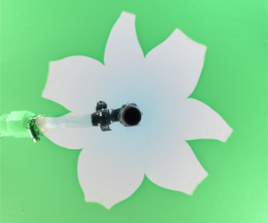
The current paper focusses on gravity currents of yield-stress fluids, which again have applications in the geosciences and engineering (Ancey Reference Ancey2007; Balmforth, Frigaard & Ovarlez Reference Balmforth, Frigaard and Ovarlez2014). In particular, the goal is to report the phenomenon illustrated in figure 1 and explore its origin. Here, a viscoplastic fluid (an aqueous suspension of Carbopol) is fed onto a flat plane. When the plane is dry, an axisymmetric gravity current is created that can be described by the viscoplastic generalization of conventional shallow-layer theory (Balmforth et al. (Reference Balmforth, Craster, Rust and Sassi2007); appendix A). However, in figure 1 the plane is wet by a thin film of water. The layer is too shallow to permit the viscoplastic fluid to float, which instead appears to displace the water and expands over the plane in the manner of a classical (shear-dominated) gravity current. Despite this, the experiments display a striking non-axisymmetric instability that creates a distinctive, flower-like pattern. The phenomenon is not restricted to the particular material used in the experiment shown in figure 1, but can be reproduced with a wide variety of water-based yield-stress and shear-thinning fluids, ranging from industrial products to household materials (such as joint compound, Xanthan gum, tomato ketchup, yoghurt, aloe vera gel and mayonnaise).

Figure 1. Images of an aqueous suspension of Carbopol (yield stress  ${{{\tau _{{Y}}}}}=12$ Pa, from a Herschel–Bulkley fit to rheometer data; see § 2.2) extruded from a pipe onto a horizontal Plexiglas surface wet by a thin film (of depth $H_w\approx 3.8$ mm) of green-coloured water. We show photographs of (a) the side view and (b) the inclined view. The top view in (c) is from above, and shows the footprint of the Carbopol identified from the image (red line); (d) displays successive outer edges, spaced by 2 s and coloured by time (from green to blue). The vent (inner radius $r_v\approx 3$mm) and feeder pipe through which the Carbopol is extruded (with flux $Q\simeq 40$ ml min $^{-1}$) is visible through the Plexiglas in the middle of the images in (a,c). The Carbopol is colourless, but appears green in (a) owing to illumination by light transmitted through the film of water. See supplementary movie available at https://doi.org/10.1017/jfm.2021.961.
The spreading structure seen in figure 1 has similarities to the patterns reported by Sayag, Pegler & Worster (Reference Sayag, Pegler and Worster2012) and Sayag & Worster (Reference Sayag and Worster2019a) in a somewhat different experiment with another complex fluid. These authors conducted experiments in which gravity currents of shear-thinning fluid (a suspension of Xanthan gum) were floated upon a bath of a denser salt solution to provide a laboratory analogue of ice shelves. The floating currents also suffered a dramatic non-axisymmetric instability in which the flow broke up into a small number of fingers. Sayag & Worster (Reference Sayag and Worster2019b) rationalized this phenomenon in terms of the linear instability of the two-dimensional extensional flow of shear-thinning (power-law) fluid. The presence of this instability for shallow, freely sliding gravity currents was confirmed by Ball & Balmforth (Reference Ball and Balmforth2021), and generalized to include flows with a yield stress.
The experiment shown in figure 1, however, resembles more closely a classical gravity current and does not appear to slide freely over the plane. Part of our purpose here is to establish more definitively that Sayag & Worster's extensional flow instability cannot be responsible for the observed patterns. For this task, we perform a number of variations on the basic experimental theme illustrated in figure 1. In particular, we compare gravity currents extruded into thin water layers with extrusions onto dry surfaces or planes covered with other, immiscible liquids. Overall, our findings are that the gravity currents into ambient water layers do not slide any more freely as those on dry surfaces, confirming that they are dominated by vertical shear (although there is a distraction due to effective slip; Barnes Reference Barnes1995). Thus, the extensional flow instability is not obviously relevant. More significantly, non-axisymmetric patterns do not form when the plane is coated by an immiscible liquid. Altogether, the experiments suggest a rather different, solid mechanical origin to the pattern formation process: the fracturing of the viscoplastic material under the stresses associated with the expansion of the current, a phenomenon observed for complex fluids in other settings such as breaking threads (e.g. Ligoure & Mora Reference Ligoure and Mora2013). That this process cannot take place on a surface that is either dry or wet with an immiscible fluid, but does arise with a film of water, points to a critical modification of the effective fracture toughness by the presence of the solvent making up the complex fluid (cf. Baumberger, Caroli & Martina Reference Baumberger, Caroli and Martina2006a,Reference Baumberger, Caroli and Martinab; Baumberger & Ronsin Reference Baumberger and Ronsin2010; Zare & Frigaard Reference Zare and Frigaard2018). This result mirrors conclusions drawn from experiments with viscoplastic fluids in Hele-Shaw cells (Ball, Balmforth & Dufresne Reference Ball, Balmforth and Dufresne2021), where similar non-axisymmetric patterns formed in radially expanding flows.
2. Experimental configuration
2.1. Set-up
Figure 2 shows a sketch of the experimental arrangement: a volume of viscoplastic fluid is extruded from below onto a flat surface coated with a thin layer of water or other fluid using a syringe pump operating at a fixed flux. The vent had an inner radius of  $r_v\approx 3$ mm unless stated otherwise. The surface was made of smooth Plexiglas, with barriers around the periphery holding the ambient fluid bath in place. Unlike Sayag & Worster, we did not adjust the density of the ambient fluid to ensure that it was denser than the extruded material, or design an overflow system to maintain the depth of the layer. For most of the experiments, the barriers were sufficiently distant that the displaced ambient fluid changed the depth by less than $10\,\%$.

Figure 2. Sketches and photographs showing the experimental arrangement: Carbopol is emplaced onto a flat surface coated with a thin layer of water by first filling and then removing a cylindrical container; a much larger volume of Carbopol is then pumped onto the surface. The vent (a pipe with an inner radius of  $r_v\approx 3$ mm) is located in the dark round hole underneath the Carbopol.
For the viscoplastic fluids that we used, any extrusion from the vent immediately forms a vertical column, much like toothpaste pushed out of a vertically held tube, which then topples over sideways to create an initially non-axisymmetric flow. To minimize any such initial non-axisymmetry, we therefore first emplaced a small volume of the viscoplastic fluid by filling, and then releasing, a cylindrical container. The preliminary dambreak formed a largely axisymmetric initial dome decorated by residual small-scale surface features stemming from the detachment of the cylinder. In figure 2 the surface features are not visible, and did not appear to significantly impact the subsequent spreading of the fluid, which, at least initially, was axisymmetric.
In some other tests we varied the arrangement illustrated in figure 2: a series of control experiments were performed without any fluid coating the surface, in a second series the underlying surface was replaced by roughened Plexiglas and a third series employed containers with different shapes for the preliminary dambreaks. Using the roughened underlying surface (with a roughness scale that we estimate to be less than  $100\ {\rm \mu}{\rm m}$, substantially smaller than the depth of any ambient fluid) allowed us to gauge the impact of any effective slip on the spreading of the viscoplastic fluid (either with or without an ambient fluid bath), whereas the tests with different containers were designed to deliberately imprint a certain non-axisymmetric initial condition.
For the bulk of our experiments, pumping was commenced ten or so seconds after the dambreak. However, we verified that the waiting time did not influence the subsequent dynamics by conducting tests (with Carbopol) in which we commenced pumping a fixed amount of time after the dambreak. The waiting times extended up to 8 min in duration which well exceeded the length of most experiments. The variation of the waiting had no discernible effect, confirming the robustness of the experimental protocol. Evidently, a prolongation of the contact between the viscoplastic fluid and water has no significant effect, suggesting that diffusion through the surface is not key (at least for Carbopol).
For quantitative measurements of our experiments we took photographs from above to image the fluid in plan view. To collect height data, we placed a mirror at 45 $^{\circ }$ to the extrusion to capture the plane projection of the side profiles. Additional photographs taken at an oblique angle provide a different perspective.
2.2. Material
For the extruded fluids we used either an aqueous suspension of Carbopol (Ultrez 21, neutralized with sodium hydroxide; density  $\rho \approx 1$ g cm $^{-3}$) or diluted ‘joint compound’ (a commercially available, kaolin-based material used for plaster board or dry wall; density $\rho \approx 1.6$ g cm $^{-3}$). Flow curves for three of the Carbopol suspensions used are shown in figure 3(a), obtained from a rheometer (Kinexus Malvern fitted with roughened parallel plates) using an up-down, controlled shear-rate ramp. The two branches of the test closely track one another, except near the yield stress, highlighting the relatively low degree of hysteresis for this material. Also shown is a fit of the down-ramp data (solid black lines) to the Herschel–Bulkley constitutive model; the resulting values for the yield stress ${{{\tau _{{Y}}}}}$, consistency $K$ and power-law index $n$ are plotted in figure 3(b) against concentration. The down-ramp of the flow curve seems most relevant for our experimental arrangement described in § 2.1: initially the Carbopol is yielded everywhere, being well sheared in the curved feeder pipe and its junctions, and then is forced to expand axisymmetrically upon extrusion onto the flat surface. We estimate typical shear rates to be $O(0.1)$ s $^{-1}$ or higher during this emplacement phase declining to $O(10^{-3})$ s $^{-1}$ at the surface and largest radii (see § 3.1 and Appendix A), after a time of order minutes.
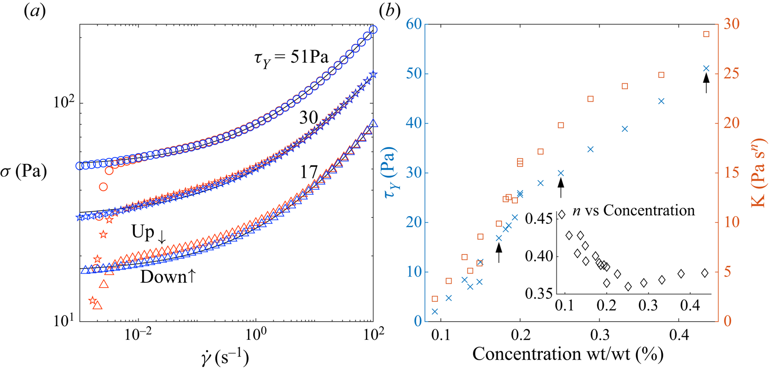
Figure 3. (a) Flow curves for Carbopol using a controlled shear-rate ramp. The up and down data are denoted by red and blue markers, respectively. The shear-rate ramp spanned the range  $[10^{-3}, 10^{2}]$ taking 10 samples each decade, and allowing 60 s to reach steady state. We show a subset of Carbopol concentrations by weight used across the experiments with Herschel–Bulkley fits (solid black lines). The resulting rheologies for all Carbopol concentrations used are given (b). The arrows indicate the Carbopol samples shown in (a).
The joint compound suspension was far from ideal in its behaviour in the rheometer, with substantial up–down hysteresis in comparison with the relatively mild behaviour seen in figure 3(a) for Carbopol. Consequently, a Herschel–Bulkley fit is much less reliable for this material, and we draw mostly qualitative observations from the experiments using it. The yield stress of the joint compound mixture was approximately  ${{{\tau _{{Y}}}}}\sim 50 - 60$ Pa.
3. Results
3.1. Control experiments without an existing fluid layer
Control experiments in which Carbopol was pumped out onto a dry surface are shown in figure 4. The extrusions remain largely axisymmetric throughout the expansion, although weak asymmetries appear at later times for the extrusion above the smooth surface (cf. Liu, Balmforth & Hormozi Reference Liu, Balmforth and Hormozi2018). The extrusions over the smooth and rough surfaces are slightly different, with the former spreading further (figure 4a) and having a different maximum depth  $H(t)$ (figure 4b), surface velocity (figure 4c) and shape $h(r,t)$ (as indicated by the dome profiles in a vertical cross-section, extracted from images taken from the side; figure 4d). Effective slip is therefore not negligible.

Figure 4. Axisymmetric spreading of Carbopol with rheology  $(n,{{{\tau _{{Y}}}}},K)=(0.43, 7.0\,\textrm {Pa}, 5.1\,\textrm {Pa}\,\textrm {s}^{n})$ at pump rate $Q\simeq 20$ ml min $^{-1}$ over rough and smooth dry surfaces. Shown are the evolution of (a) the average radial position of the outer edge $R_{av}(t)$ and (b) the central (maximum) dome depth $H(t)$, both plotted against extruded volume $Qt$, and (c) the radial surface velocity $u_{surf}$ and (d) dome profiles at $Qt=84$ ml. The solid line shows a numerical solution of the shallow-layer theory of Appendix A, beginning from an equilibrium dome of volume 6 ml; the dashed line shows the solution without an initial dome, and the dots in (c) plot equation (A7). The inset in (a) shows the degree of non-axisymmetry $\varLambda$, and those in (b) display photographs of two final domes. Surface velocities in (c) are inferred from placing tracer particles on the Carbopol surface and measuring their horizontal displacement.
We quantify the degree of non-axisymmetry using the diagnostic,
 \begin{equation} \varLambda(t) =\frac{R_{max}(t)-R_{min}(t)}{R_{av(t)}}, \end{equation}
where  $R_{max}(t)$ and $R_{min}(t)$ denote the maximum and minimum radii of the outer edge and the average radius is defined by $R_{av}=\sqrt {A/{\rm \pi} }$, with $A(t)$ denoting the projected area of the Carbopol on the underlying plane (figure 4(a) inset). Note that figure 4 includes results from three tests for both the rough and smooth surfaces, providing some idea of how measurement errors and experimental uncertainties impact the reproducibility of the experiments.
The figure also compares the results with the predictions of a shallow-layer theory for a gravity current of viscoplastic fluid advancing over a no-slip surface (Balmforth et al. (Reference Balmforth, Craster, Rust and Sassi2007); appendix A). The theory qualitatively reproduces the experiments over the rough surface, even though the domes are not particularly shallow; the relative discrepancies are of order the aspect ratio (which is approximately  $\frac 13$), as expected from the underlying asymptotic analysis. More detailed comparisons of experiments and shallow-layer theory are presented by Andreini, Epely-Chauvin & Ancey (Reference Andreini, Epely-Chauvin and Ancey2012), Chambon, Ghemmour & Naaim (Reference Chambon, Ghemmour and Naaim2014) and Freydier, Chambon & Naaim (Reference Freydier, Chambon and Naaim2017) for other free-surface flows of viscoplastic fluid over dry surfaces. Liu et al. (Reference Liu, Balmforth, Hormozi and Hewitt2016); Liu, Balmforth & Hormozi (Reference Liu, Balmforth and Hormozi2018, Reference Liu, Balmforth and Hormozi2019) also provide comparisons with numerical solutions of the full equations of motion. Overall, for these shallow flows, there is broad agreement between theory and experiments. Thus, a Herschel–Bulkley rheology is sufficient to describe the dome dynamics, other rheological effects having less impact, and the shallow-layer theory provides a useful guide to the shape, velocity and stress fields.
3.2. Extrusions into a water layer
3.2.1. Carbopol
In stark contrast with the extrusions in air, a dramatic non-axisymmetric instability is observed during the radial outflow when an existing water layer surrounds the Carbopol. Figure 1 shows a sample experiment when Carbopol with yield stress  ${{{\tau _{{Y}}}}}=12$ Pa is pumped into an existing layer of water of depth $H_w=3.8$ mm. Shown are photographs of the surface of the Carbopol at the end of the test, together with a series of snapshots of the outline of the outer edge of the dome, taken every 2 s and extracted by processing images taken from above. As described in § 2.1, the test begins from a dome formed by an axisymmetric dambreak. Once the pumping of Carbopol is commenced, this dome begins to spread out, initially axisymmetrically, as illustrated by the first few snapshots of the outer edge (see also the final image in figure 2). A short time later, however, sharp and localized $v$-shaped splits or ‘fractures’ of the outer edge appear where there is contact with the surrounding water. These defects divide up the radial outflow and prompt the formation of distinctive fingers. As the fingers extend, they leave behind the tips of the fractures, and the outflow settles into a petal-like pattern. During the later stages of evolution, the fingers adjust with their front edges flattening out, and the fractures shifting in angle to allow the development of a somewhat more regular pattern. A video of the full experiment is available in the supplementary materials.
Finer details of the fractures as they form in a second experiment with a different Carbopol (with  ${{{\tau _{{Y}}}}}=19$ Pa) are shown in figure 5. Note that averages inherent in the image processing, optical distortions and the viewing perspective all contribute to obscuring the three-dimensional structure of the crack. Nevertheless, the appearance of each crack looks very much like that of a fracture through a solid.

Figure 5. Crack evolution in an experiment with Carbopol of rheology  $(n,{{{\tau _{{Y}}}}},K)=(0.39,19\,\textrm {Pa}, 12\,\textrm {Pa}\,\textrm {s}^{n})$, pumped at a rate $Q\simeq 20$ ml min $^{-1}$ into a water layer of depth $H_w=3.8$ mm. The evolving outer edge is plotted in (a), equally spaced at intervals of ${\rm \Delta} t=1$ s and colour coded in time (green to blue). The grey solid line plots the initial condition; the dashed line indicates where the pipe from the pump obscures the image. A photograph taken from an oblique angle is displayed in (b), and shows the distortion of an underlying grid of light lines. In (c) we plot magnifications of the outline of the fracture indicated in (a), and in (d) we translate and rotate these profiles (giving coordinates $(x_c,y_c)$) to align the tip of the crack. From the average of the $v$-shaped sections of these profiles, we define a master curve, as plotted by the solid black line. In (e) we plot master curves for all four of the fractures that appear in the test (the fourth fracture has not yet appeared in (a,b)), as well as for four more cracks appearing in another experiment with the same Carbopol (giving 16 curves on this $(x_c,|y_c|)$ plot). The red dashed lines indicate angles of $20^{\circ }$ and $35^{\circ }$. In (f) we plot master curves of fractures from two experiments with Carbopol rheologies $(n,{{{\tau _{{Y}}}}},K)=(0.43,7\,\textrm {Pa}, 5.1\,\textrm {Pa}\,\textrm {s}^{n})$ (blue lines, 8 fractures) and $(n,{{{\tau _{{Y}}}}},K)=(0.39,39\,\textrm {Pa}, 24\,\textrm {Pa}\,\textrm {s}^{n})$ (red lines, 2 fractures), both with the same $Q$ and $H_w$.
Due to the non-axisymmetric spreading of the current, the roots of the fractures move in both radius and angle. As illustrated in figure 5(c,d), if we translate and rotate the local outline of the edge so that the crack tip becomes fixed in the crack-orientated coordinates  $(x_c,y_c)$, the fracture becomes aligned to highlight its characteristic $v$-shape and an underlying ‘master profile’. Master profiles for all four of the cracks that appear in the experiment of figure 5 are illustrated in (e), along with four more of these profiles from the cracks appearing in a second test with the same Carbopol (here, both sides of the profiles are plotted using the crack-orientated coordinates $(x_c,|y_c|)$, to give a total of sixteen curves). Although the fractures appear at different angular positions and times relative to one another, the master curves show little variation near their tips and are reminiscent of the profile of a blunted crack in a solid. A similar collapse of the profiles of a breaking thread of another complex fluid is presented by Tabuteau et al. (Reference Tabuteau, Mora, Ciccotti, Hui and Ligoure2011). In fracture theory, a characteristic measure of the displacement opening a crack is defined by considering the intersection of the edges with a right-angled triangle centred at the tip; sometimes proposed as a material parameter, this ‘crack opening displacement’ would be a fraction of a millimetre for the master curves shown in figure 5(e) (as in Tabuteau et al. Reference Tabuteau, Mora, Ciccotti, Hui and Ligoure2011). Interestingly, the shape of the tip of the master curves is much the same for cracks from experiments for different Carbopols (see figure 5f), suggesting any such material characterization is a weak function of concentration. Further from the crack tip, the master profiles all spread out where these local $v$-shaped splits must match on to the surrounding viscoplastic flow; over these sections of the master curves, the variability between cracks in the same test is comparable to that between different experiments.
Although the Carbopol domes are much deeper than the ambient water layer, there is a significant climb of the waterline up these structure through capillary effects. This climb can be seen in figure 5(b), which shows a test in which a grid of lines was imaged through the fluids. The distortion of the grid reflects the surface topography of the water and Carbopol. In combination with other visual observations of light reflections on the water surface and from experiments where dye or fluorescein was added to the water, these distortions suggest that the water climbs significantly up the crack faces, close to the top of the fractures. The dye and fluorescein also failed to detect any residual water layer underneath the Carbopol, suggesting an almost complete displacement of the ambient water layer.
Figure 6 shows a longer experiment in which three fractures form to guide the subsequent non-axisymmetric expansion. Once the front edges of the fingers have largely flattened, these structures are largely pushed out radially with little further change of shape (tracking tracers added to the fluid confirms this plug-like flow). The material further along the fingers must therefore be held close to the yield stress, with fresh fluid flowing past the fracture tips filling in the gaps between the fingers to create the distinctive petal-like pattern. Figure 6(e) plots the corresponding snapshots of the profile of the dome in a vertical cross-section. Although the centre of the dome noticeably deepens during the extrusion, the fingered regions remain much closer to uniform depth once established, in line with the nearly constant shape of the fingers observed from above.

Figure 6. A Carbopol extrusion with rheology  $(n,{{{\tau _{{Y}}}}},K)=(0.37,39\,\textrm {Pa}, 24\,\textrm {Pa}\,\textrm {s}^{n})$ into a water layer of depth $H_w=3.8$ mm at flux $Q\simeq 20$ ml min $^{-1}$ showing time series of (a) $R_{max}$, $R_{min}$, $R_{av}$ and $H$ (all in cm), and (b) $\varLambda = (R_{max}-R_{min})/R_{av}$ (plotted against extruded volume $Qt$). Snapshots of the outer edge, colour coded by time and spaced by 20 s, are shown in (c), then replotted in (d) with a scaling of $R_{max}$. The snapshots with $V<33$ ml are plotted in grey. Snapshots of the evolving side profile are plotted in (e), colour coded by time and spaced by 20 s. The grey dashed line shows the water layer depth; just above this level the Carbopol profile cannot be reliably detected. The solid black line in (c) indicates the plane of projection of the side profiles, viewed in the direction given by the arrow.
After the fractures are established, figure 6(a) further illustrates how the maximum, minimum and mean radii all increase with time and largely keep pace with one another. This feature is brought out in more detail by plotting the non-axisymmetry measure  $\varLambda (t)$ in (3.1) (see (b)), which now measures a typical, relative crack length. The measure levels off after the initial adjustment, and suggests that pattern evolves in a somewhat self-similar manner. By scaling distances by the maximum radius $R_{max}$, we illustrate that similarity in (d); the dominant changes arising from expansion are now largely suppressed, exposing the residual non-self-similar evolution stemming mostly from the advance of the nearly rigid finger tips and the filling of the gaps between the nearly rigid fingertips.
Extrusions of the  ${{{\tau _{{Y}}}}}=51$ Pa Carbopol into a water film above a smooth Plexiglas plate are compared more quantitatively with a control experiment in air in figure 7. The presence of ambient water makes little difference to the average rate of expansion, as quantified by $R_{av}$ (see (a)). Evidently, the ambient water neither lubricates the dome's expansion nor modifies the effective slip, in line with the lack of any discernible water underneath. Thus, the dome does not slide significantly more over the underlying wetted plane than it does over the dry surface, implying that an extensional flow instability cannot be responsible for the development of non-axisymmetry.

Figure 7. Carbopol extrusion over a smooth surface with an ambient water layer of depth  $H_w=3.1$ mm (repeated three times). Shown are (a) the average radial position of the outer edge $R_{av}(t)$ (plotted against extruded volume $Qt$), (b) the central (maximum) dome depth $H(t)$, (c) the degree of non-axisymmetry $\varLambda$ and (d) the final dome profiles. The inset in (b) plots snapshots of the detected interface spaced by 20s and coloured by time (from red to blue). A control experiment in air is plotted as the solid line, and the dashed line again shows the prediction of shallow-layer theory. $Q\simeq 20$ ml min $^{-1}$; $(n,{{{\tau _{{Y}}}}},K)=(0.38, 51\,\textrm {Pa},29\,\textrm {Pa}\,\textrm {s}^{n})$.
The maximum depth  $H(t)$ and depth profile $h(r,t)$ (plotted in figure 7b,d) show more noticeable differences between the extrusions over the wet and dry smooth surfaces: the fingers at the edge of the domes extruded into water are again evident in figure 7(d) as the smaller mounds pushed ahead of the main dome. The associated rearrangement of fluid impacts the cross-sectional profile, slightly lowering the dome in comparison with the test with dry Plexiglas.
Figure 7 shows the results from three repetitions of the test over the smooth surface. As emphasized by the outlines of the outer edges included as insets in (b), the patterns created are not identical. In particular, the patterns differ in the positions, moment of initiation and number of fingers, even though the rate of expansion and side profiles are similar. Evidently, there are multiple possible states to which the flow may evolve, a feature that unavoidably introduces awkward additional variability into the results. Imperfections and inhomogeneity are likely the culprits in randomizing the selection of the pattern for each test; we attempt to minimize the effect of these inconveniences by more carefully controlling the initial condition in § 3.5.
3.2.2. Joint compound
Pattern formation like that shown in figures 1 and 6 characterized every single test in which Carbopol was extruded into an ambient water layer, although the quantitative details of the patterns varied with the experimental parameters (see § 3.4). Similar non-axisymmetric patterns appeared in extrusions with joint compound; see figures 8–10. Again, such extrusions remain axisymmetric in the absence of an ambient liquid (figure 8a), but develop flower-like, nearly self-similar fracture structures when extruded into water (figures 8(b,c) and 9(d,e)). The number of fractures is higher and the pattern more regular with joint compound, but the cracks are shorter in length. The non-axisymmetry measure (or relative crack length)  $\varLambda$ also evolves a little differently (comparing figure 9(c) with 6(b)).

Figure 8. A collage of final images from tests with the joint compound suspension extruded (at  $Q\simeq 20$ ml min $^{-1}$) in (a) air, (b) water, (c) dark blue ink and (d) water with varying depth ( $H_w=3.5$, 7, 14, 21 mm for the first four; the joint compound is completely submerged in the last picture). In (a,b), a volume of $V=100$ ml is extruded; $V=60$ ml for (c,d).

Figure 9. Joint compound extrusions with varying pump rate with an ambient water layer of depth for  $H_w=3.5$ mm. Time series of (a) the average radius $R_{av}$, (b) the mean, maximum and minimum radii for $Q\simeq 5$ ml min $^{-1}$ and (c) the non-axisymmetry measure $\varLambda$, where time $t$ is measured from commencement of pumping. The green dashed line in (b) shows the radius of the axisymmetric extrusion in air. In (d) we show snapshots of the outer edge at equally spaced intervals, coloured with time and spaced by 80, 40, 20 and 10 s from left to right, for the experiments with the pump rates indicated. The interfaces are scaled by the maximum radius $R_{max}$ in (e). In both (d,e) the interfaces for $Qt<33$ ml are plotted in grey.

Figure 10. Crack formation in joint compound extrusions, for  $H_w=3.5$ mm and $Q\simeq 5$ ml min $^{-1}$. In (a) we plot snapshots of a forming fracture in the outer edge, equally spaced and colour coded by time. The evolving outer edge as a whole is plotted in (b) with the same colour scale as in (a), and the distinguished fracture is indicated by the red triangle. The grey line plots the initial condition. In (c) we show the final photograph of the sequence.
The opaque nature of the joint compound is helpful in gauging whether any water (when dyed) remains underneath the dome as it is extruded. Figure 8(c) shows a test in which dark ink was added to the water, displaying photographs taken from both above and below the extruded dome. The faint blue discolouring underneath the fingertips highlights how a residual water layer persists below the extruded fluid. However, the coloured layer is plainly thin and very restricted radially, disappearing before reaching the crack tips. Nevertheless, unlike the Carbopol, the time series of the average radius  $R_{av}(t)$ in figure 9(b) does suggest some additional lubrication of the joint compound by the ambient water.
Another interesting observation arises when the water level in the ambient bath is raised substantially so that it is no longer much shallower than the dome (the arrangement for most of our experiments). With Carbopol, such extrusions were problematic, as the dome, if too submerged, would float up away from vent on the commencement of pumping, destroying the experiment. The denser joint compound, however, still spreads over the underlying plane even if completely submerged. The series of images in figure 8(d) show typical results with substantially raised water levels. Once the water level was increased, more fractures formed. However, rather than appearing as localized defects at the outer edge, the entire wetted surface of the joint compound appeared to crumble under the extensional stresses associated with the radial expansion (the surface stresses predicted theoretically are provided in Appendix A), generating a complicated, rough surface texture. Only where the dome remained above the waterline did the surface remain smooth, with completely submerged domes taking on a fully roughened appearance.
Thus, the surface of the joint compound appears to have little integrity when in contact with water, suggesting that interfacial effects might be at the heart of the fracture patterns rather than a bulk hydrodynamic instability. Indeed, although Carbopol experiments with deep ambient fluid layers were problematic, it was still possible to conduct tests with water levels that climbed higher up the domes. In such tests, fractures formed quickly and disruptively, no longer being restricted to the outer edge. Instead, the Carbopol appeared to tear across the upper surface wherever water was available, generating much more complicated fingering patterns with an irregular network of cracks threaded throughout the extrusion.
3.2.3. Roughened plates
In § 3.1 it was noted that Carbopol extrusions without a water layer were sensitive to the underlying surface as a result of effective slip. To examine whether the roughness of surface also impacted the non-axisymmetric patterns in extrusions with a shallow water layer, we also conducted tests with roughened Plexiglas plates. The results were surprisingly different, as illustrated in figure 11: although small cracks appeared at the outer edge where the Carbopol was in contact with water, these features lengthened significantly less, remaining peripheral decorations to the dome. Evidently, the elimination of effective slip by the roughening of the plates impacts the propagation of the cracks.

Figure 11. Carbopol extrusions over a smooth and rough surface with a pre-existing water layer ( $H_w=3.8$ mm; $Q\simeq 20$ ml min $^{-1}$; ${{{\tau _{{Y}}}}}=12$ Pa). (a) Shows outlines of the outer edge, spaced by 10 s and colour coded by time; (b) plots $\varLambda$ against $Qt$.
$Qt$.
3.3. Different ambient fluids
To explore further the possibility that interfacial effects drive the non-axisymmetric patterns, we conducted tests with a variety of different ambient fluids. First, it is well documented that the rheology of Carbopol (although not the joint compound mixture) is sensitive to pH, and so it is conceivable that an acid–base imbalance might have prompted the patterns. In fact, the tests shown in figures 1 and 5 use local tap water for the ambient bath, which is controlled by local city utilities to have a pH of approximately 7.5, whereas the Carbopol suspension is neutralized by sodium hydroxide as part of its preparation. As a check on whether this pH difference had any impact, we repeated a number of the tests using a bath of distilled water with the same pH as the Carbopol. There was no noticeable effect on the extrusion patterns, indicating that pH differences of order 0.5 are insignificant.
We also conducted suites of tests in which we dissolved either salt or sugar in the ambient water bath. The addition of salt (NaCl) with concentration of 1 % or 2 % by weight increases the density by  $0.5$ or 1 % (respectively) without substantially changing the viscosity. The ambient bath is then noticeably denser than the Carbopol, which might influence the displacement of residual salty water from the surface and change the degree of lubrication of the dome. There is also a possibility that the salt could interact with the Carbopol microstructure to alter the rheology. Indeed, by dropping small volumes of dyed Carbopol into the salt solution, one could directly observe an interfacial interaction in which coloured water appeared to be drawn osmotically from the Carbopol into the salt solution causing the local gel structure to deteriorate (sprinkling dry salt onto the Carbopol has even more dramatic results). Nevertheless, such interfacial effects occurred over time scales of 10 min, rather longer than our extrusion tests. In fact, as reported in figure 12, neither the change in buoyancy nor interfacial interaction appeared to play a role in the pattern formation process.

Figure 12. (a) A collage of tests with different ambient fluids showing the detected interfaces, coloured by time and spaced by 10 s. Top row: 8.0 Pa Carbopol ( $V=100$ ml) with water, water with 1 %wt salt ( $\sim$0.5 % increase in density) and water with 2 %wt salt ( $\sim$1 % increase in density). Middle row: 19 Pa Carbopol ( $V=60$ ml) with water, 20 % wt sugar solution (1.1 g cm $^{-3}$; 2 mPa s), 40 % wt sugar solution (1.2 g cm $^{-3}$; 6 mPa s) and 60 % wt sugar solution (1.3 g cm $^{-3}$; 60 mPa s). Lower row: 17 Pa Carbopol ( $V=100$ ml) with air, water, paraffin oil (0.8 g cm $^{-3}$; 3 mPa s) and mineral spirits (0.8 g cm $^{-3}$; 1 mPa s). Time series of average radius $R_{av}$ and the non-axisymmetry measure $\varLambda$ are plotted in (b–g). ( $Q\simeq 20$ ml min $^{-1}$ and $H_w=3.5$ mm).
The addition of sugar up to concentrations of 20 %, 40 % or 60 % by weight incurs more significant changes in both density and viscosity (increasing density by 10 % to 30 %, and the viscosity up to 2, 6 and 60 mPa s, respectively). As shown in figure 12, however, the qualitative details of the non-axisymmetric patterns were no different (although there are some quantitative modifications, such as in the number of fractures and the rate at which fractures form due to the addition of sugar). Again, therefore, the phenomenology is insensitive to both the presence of chemical impurities or a change in the density and viscosity of the ambient fluid. Despite this, there was one noticeable difference in the experiments with salt or sugar water: at the higher concentrations, the interface between the Carbopol and water appeared to become contaminated or rougher at later times, suggestive of some sort of a localized interfacial interaction.
Although variations in the properties of water-based ambient baths had little effect, when we extruded Carbopol or joint compound into films of immiscible fluids, there were striking differences. Figure 12 displays the results for extrusions into two immiscible liquids of comparable viscosity to water (a paraffin-based oil and mineral spirits). Both extrusions show little development of non-axisymmetry, except perhaps minor ones at late time, with the outflow very similar to extrusion onto the dry surface. Thus, the fracture pattern can be entirely eliminated by replacing the ambient water with an immiscible liquid of comparable viscosity. Similar results were found in tests with the joint compound. Note that the density of the paraffin oil and mineral spirits is a little less than the Carbopol. However, the ambient baths are relatively shallow and the tests with salt and sugar water suggest that minor density differences do not matter.
3.4. Trends with varying experimental parameters
For Carbopol extruded into a water layer, the extrusion pattern depends on the ambient water depth  $H_w$, flux $Q$ and rheology (which we identify using the yield stress ${{{\tau _{{Y}}}}}$). An impression of this dependence is provided in figure 13, which shows evolving extrusion edges from suites of tests in which we varied one of these three experimental parameters. More detailed results from these series of tests are summarized in Appendix B.

Figure 13. Carbopol extrusions in water with varying ambient depth  $H_w$, flux $Q$ and rheology (identified by yield stress ${{{\tau _{{Y}}}}}$), showing snapshots of the outer edge (spaced by 20 s unless otherwise indicated). In the top row, the water depth varies as indicated, with ${{{\tau _{{Y}}}}}=8.0$ Pa and $Q\simeq 20$ ml min $^{-1}$. For the middle row, the flux varies with ${{{\tau _{{Y}}}}}=8.0$ Pa and $H_w=3.8$ mm (outlines spaced by 80, 40, 20, 10 and 10 s from left to right). Along the bottom row, the rheology varies, with $Q\simeq 20$ ml min $^{-1}$ and $H_w=3.8$ mm. The insets in the top two rows show corresponding outlines of the second series of tests for varying $H_w$ and $Q$ with ${{{\tau _{{Y}}}}}=51$ Pa; in the lower row, the insets show repetitions of each test in the series with varying ${{{\tau _{{Y}}}}}$. These inset outlines are plotted with half of the spatial scale and with colour coding from green to blue.
The trends seen along the first two rows in figure 13 highlight how the strength of the non-axisymmetry increases with both increasing water depth and decreasing flux, as also evident for the joint compound tests in figure 9(d). A decrease in yield stress leads to a less obvious change in the degree of asymmetry although it does impact the number of fingers. The time series of the relative length of the fingers  $\varLambda$ reported in figure 18 of Appendix B demonstrates more quantitatively these features. Also displayed in the lower row of figure 13 is a second series of outlines showing repetitions of each of the tests with varying ${{{\tau _{{Y}}}}}$. The comparison between the two sets of tests in this row again emphasizes the vagaries in the shape of the pattern possible even for the same Carbopol and extrusion conditions. As evident from figures 6(b), 7(c), 11(b) and 12(c,e,g) (see also figure 18d–f), the measure $\varLambda = (R_{max}-R_{min})/R_{av}$ roughly levels off after the appearance of the non-axisymmetric pattern. A more compact diagnostic of the non-axisymmetry can therefore be defined by averaging $\varLambda$ over this self-similar-like regime (which we observe to be broadly identified by the criterion, $V>33$ ml, for all the experiments). This diagnostic, together with visual observations of the number of fractures, is plotted in figure 14 against the variable experimental parameters, revealing more concisely the experimental trends. The estimate for the number of fractures is a little subjective, given that these features sometimes appear but fail to grow and influence the radial outflow; in figure 14, the weaker, inconsequential cracks are either discarded, to generate a lower bound, or included to furnish an upper bound. For joint compound, the situation is a little different, with the majority of the initial cracks failing to develop: figure 10 shows the early-time evolution of the test at 5 ml min $^{-1}$ that appears in figures 8 and 9, and highlights the multitude of initial incipient defects.

Figure 14. The number of cracks and average non-axisymmetry measure  $\langle \varLambda \rangle$ (over volumes $33< V<100$ ml) against (a,d) water depth $H_w$ ( $Q\simeq 20$ ml min $^{-1}$, ${{{\tau _{{Y}}}}}=8.0, 51$ Pa), (b,e) flux $Q$ (
$Q$ ( $H_w=3.8$ mm, ${{{\tau _{{Y}}}}}=8.0, 51$ Pa) and (c,f) yield stress ${{{\tau _{{Y}}}}}$ ( $H_w=3.8$ mm, $Q\simeq 20$ ml min $^{-1}$). In (g) the data are collapsed by plotting the non-axisymmetry measure against the stress ratio $\mathcal {S}$ defined in (4.1) (the dashed line shows $\langle \varLambda \rangle =\frac {1}{5}{\mathcal {S}}$); the markers correspond to the data in (a–f) except for eight additional experiments that are plotted as green inverted triangles. The error bars in (d–f) correspond to the maximum and minimum values of $\varLambda (t)$ over volumes $33< V<100$ ml. For the number of cracks, two estimates are shown (connected by a line, if different): an upper bound based on the total number of cracks that could be seen, and a lower bound that discards the cracks that did not develop into long fractures organizing the pattern. In (c), data from all the experiments are included as grey symbols. The grey line in (a–f) represents the results from the tests with controlled initial conditions in figure 15(b,c). The trends $\langle \varLambda \rangle =H_w/1$ and $h_w/1$ cm are indicated in (d), where $h_w=H_w+H_{cap}$ and the capillary rise $H_{cap}=1.6$ mm.
Different measures of the non-axisymmetric pattern could be extracted using a Fourier transform of the outlines of the outer edge (cf. Sayag & Worster Reference Sayag and Worster2019a): the angular wavenumber at the peak of the spectrum gives roughly the same measure as counting the number of fractures, and is free of any subjectivity, whereas an alternative to  $\varLambda$ could be defined from the power in the non-axisymmetric modes. However, the interpretation of the main peak in the spectrum is obscured when the patterns are less regular and the fingers are unequally spaced; our count of the number of fractures is more direct and easily interpreted, even if it is occasionally difficult to identify.
Note that the number of cracks in the Carbopol domes is insensitive to all the experimental parameters except at lowest concentrations ( ${{{\tau _{{Y}}}}}<10$ Pa); between two and five cracks appear for all the tests with the other suspensions, showing no trend with $H_w$, $Q$ and ${{{\tau _{{Y}}}}}$ (cf. the red points in figure 14(a,b), and figure 14(c) which includes results from all the tests). The number of fingers does not, therefore, provide a particularly clear diagnostic for our experiments.
The trends in figure 14 also obscure how the pattern formation process disappears as the viscoplastic fluid is made more Newtonian. At the lowest Carbopol concentrations, it appears as though the fracture phenomenon becomes stronger with more fractures forming, rather than disappearing. Instead we observe that, as one approaches the Newtonian limit, the Carbopol becomes progressively weaker, with the interface losing more of its integrity and looking increasingly like that of submerged joint compound. In other words, the fracturing instability is always present but the two fluids become increasingly indistinguishable at low Carbopol concentration.
3.5. Non-axisymmetric initial conditions
As a final variation of the experiment, we modified the initial dambreak condition, imprinting a prescribed non-axisymmetric structure on the dome from which the extrusion commenced. In particular, we employed cylinders containing sharp protruding fins positioned at  $n_0$ equally spaced angular intervals around the inner circumference, as sketched in figure 15(a). When the cylinder was lifted off to form the initial dambreak, the fins cut through the depth of the Carbopol to create pre-existing lines of weakness. These defects were given insufficient time to heal by commencing the extrusion a few seconds after each dambreak. Two cylinders with different radii and filled to different initial volumes were used such that the initial height of the dambreak, or equivalently height of the initial weakness, was roughly the same.

Figure 15. Carbopol extrusions (with flux  $Q\simeq 20$ ml min $^{-1}$) in which $n_0$ cracks are initiated at $t=0$ by using a cylinder fitted with sharp internal fins, as illustrated in (a). Shown in (b) are snapshots of the outer edge (rheology $(n,{{{\tau _{{Y}}}}},K)=(0.39,19\,\textrm {Pa},13\,\textrm {Pa}\,\textrm {s}^{n})$), colour coded by time and spaced by 20 s, with the number and orientations of the fins indicated. The first example shows an extrusion in air; the subsequent tests have an ambient water layer of depth $H_w=3.5$ mm. The radius of the cylinder is $r_0=1.15$ cm and the vent had an inner radius of $r_v=3.8$ mm. In (c,d) we show the number of cracks formed $n$ against the number of cracks initiated $n_0$ for the following Carbopol yield stresses ${{{\tau _{{Y}}}}}$, initial cylinder radii $r_0$ and initial volume $V_0$: (c) $r_0=1.15$ cm, $\tau_Y=19$ Pa, $V_0=6$ ml; and (d) $r_0=2.5$ cm, $\tau_Y=28$ Pa, $V_0=14$ ml ( $Q\simeq 20$ ml min $^{-1}$, $r_v=3.8$ and $H_w=3.5$ mm). Some of the tests are repeated, and two other shapes are included in (a), 6 and 7 pointed stars, with the same initial volume $V_0$ as the cylinders with protruding fins.
Despite the initial failure surfaces, the Carbopol expanded axisymmetrically to eliminate any non-axisymmetric defects when the test was conducted over a dry surface (figure 15b). With an ambient water film, however, the fins provided nucleation sites for fractures, biasing the subsequent development of the non-axisymmetric pattern. For both cylinders, when  $2< n_0<6$ the fracture pattern maintained the angular symmetry imposed by the initial condition, and the number of cracks $n$ remained equal to $n_0$. For $n_0<3$, more cracks typically appeared at the outer edge a short while after the commencement of pumping to create a pattern with $n>n_0$. When $n_0>5$, some of the initial cracks usually failed to develop any further and closed up, leading to a pattern with $n< n_0$. A summary of the various tests is shown in figure 15(c,d), which plots the final number of cracks against $n_0$. Similar results were obtained when smooth sided containers with other shapes were used (results for six and seven-point stars are included in figure 15c).
The range of  $n$ seen for the experiments of § 3.4 is shown by the grey shaded region in figure 15(c), excluding the series with ${{{\tau _{{Y}}}}}=8.0$ Pa where the flux and water depth have a clear impact on the number of cracks (figure 14a,b). The range is consistent with the size of the stable range identified by the experiments with controlled initial conditions. Evidently, there is a preferred range of angular wavenumbers for the extrusion patterns, with the tests commencing from axisymmetric initial conditions sampling the set of stable crack numbers. The multiplicity of possible patterns underscores a good fraction of the variability seen in figure 14, as indicated by the addition of the results for controlled initial conditions to the summary plot.
4. Discussion
4.1. Critique
The lack of discernible lubrication of the dome, the pronounced dependence of the non-axisymmetric patterns on water depth and their elimination when the plane is coated by an immiscible liquid all indicate that Sayag & Worster's extensional flow instability is not responsible for our experiments. Indeed, it is hard to imagine what other bulk hydrodynamic instability could be relevant.
Similarly, the experiments argue against any explanation based on the rheological behaviour of Carbopol near its yield stress: besides failing to account for the impact of ambient water, the fractures appear early in the extrusion, where the fluid is already fully yielded and shear rates are of order  $0.1\,\textrm {s}^{-1}$ (cf. § 2.2). The shear rates subsequently decline, but never build back up, precluding any effect of the mild hysteresis seen in the flow curves for Carbopol (figure 3). In any event, the finger patterns appear in much the same way for all the concentrations of Carbopol that we have used and for a range of other viscoplastic fluids, all with widely different degrees of thixotropy and other non-ideal rheologies.
In fact, the local  $v$-shaped splits appearing at the outer edge that divide the flow into fingers appear more similar to a solid-like tearing of the fabric of the viscoplastic fluid. Indeed, our tests in which the patterns are controlled by employing initial conditions with prescribed asymmetry are similar to previous explorations of the punctures in solid sheets (Vermorel, Vandenberghe & Villermaux Reference Vermorel, Vandenberghe and Villermaux2010). These authors examine the crack patterns created as a cone is pushed through a metal sheet, beginning from a non-axisymmetric initial condition containing a prescribed number of fractures. They record the length and number of the fractures that characterize the final puncture, finding results for the latter like those we report in § 3.5. To complement these experimental results, Vermorel et al. (Reference Vermorel, Vandenberghe and Villermaux2010) employ an energy minimization argument based on Griffith's classical crack theory (Griffith Reference Griffith1921), taking the crack length and number as optimization parameters, precisely the two diagnostics we employ for our tests with Carbopol in § 3.4.
Unfortunately, any equivalent approach for the current experiments runs into immediate challenges: Griffith's theory considers the energetics of a crack embedded within a linearly elastic solid. This purely elastic model trades off the release in stored elastic energy against the increase in new surface energy. Subsequent developments introduce a small plastic zone around the crack tip to regularize any stress singularities whilst retaining linear elasticity elsewhere. But, for our experiments, not only are deformations around the crack tips visibly large, the entire dome is is yielded and apparently in a state of viscoplastic expansion, as suggested by our experiments in air which are captured by shallow-layer theory for a viscoplastic fluid.
Carbopol is often assumed to be close to an ideal viscoplastic fluid, based primarily on flow curves like those displayed in figure 3(a). However, elastic effects have been reported above and below the yield stress (e.g. Piau Reference Piau2007; Balmforth et al. Reference Balmforth, Frigaard and Ovarlez2014; Bonn et al. Reference Bonn, Denn, Berthier, Divoux and Manneville2017; Ovarlez Reference Ovarlez2019; Younes et al. Reference Younes, Himl, Stary, Bertola and Burghelea2020). It is therefore unclear how much elastic energy is released as stresses are relieved by crack formation, and the situation appears more analogous to the ductile (i.e. plastic) failure of metal plates (Wierzbicki & Thomas Reference Wierzbicki and Thomas1993; Wierzbicki Reference Wierzbicki1999). The calculation of the energetic penalty paid by the production of new surfaces is also problematic: Carbopol is water based and the residual surface tension (surface energy per unit area) at an interface with water is not known.
An equally serious issue is illustrated by a pronounced dependence of the experimental patterns on flux (see figures 18(d) and 14(b,e)), which all by itself rules out any rate-independent theory for an elastic solid like Griffith's or plastic generalizations of it (Wierzbicki & Thomas Reference Wierzbicki and Thomas1993; Wierzbicki Reference Wierzbicki1999). In fact, not only is the advance of the cracks rate dependent, but once established, the cracks largely move in tune with the expansion of the bulk of the fluid (the relative crack length  $\varLambda$ becomes roughly independent of time). In other words, the cracks appear to be controlled by the large-scale flow dynamics at late times, rather than any local fracture properties. This control is further reflected by the dependence on whether the underlying surface is rough or smooth, which implies that the opening of the cracks is limited by the ability of the viscoplastic fluid to deform over the surface (another result that cannot be explained from the Griffith's perspective).
4.2. Synthesis and speculation
With the preceding critique in mind, we now attempt to synthesize our main observations and quantitative measurements into a broad image of the dynamics at the heart of the non-axisymmetric patterns. First, the availability of ambient water is evidently a key aspect. Against a perfectly wettable vertical wall, water is expected to rise under capillary stresses to a height of  $\sqrt {2\gamma /\rho g}\approx 4$ mm. Thus, given the aqueous composition of Carbopol and the relatively steep periphery, the ambient water film surrounding an expanding viscoplastic dome is expected to climb to a height of $h_w=H_w+H_{cap}$ up the top surface, where $H_{cap}=O(1)$ mm. If the material then fractures most of the way up to the resulting waterline, the fingers created by the cracks should have a similar depth to $h_w$. Our observed side profiles are indeed consistent with this expectation (figures 6, 7 and 18), and the relative crack lengths $\langle \varLambda \rangle$ in figure 14(d) are directly proportional to $h_w$ with $H_{cap}\approx 1.6$ mm.
Once liberated by fracture, the fingers are pushed out in a largely planar fashion, with stresses lowered to near the yield stress such that the fingers subsequently deform weakly. The raft-like fingers then flow over the underlying plane, becoming sensitive to whether that surface is roughened or smooth, and with the additional drag associated with the roughened plane more effectively limiting fracture lengths (figure 11).
The shallow-layer theory outlined in Appendix A establishes that the outer edge of an axisymmetric dome is in a state of angular expansion, but also radial and vertical compression. The associated plastic stresses suggest that there is a net dissipation rate of order  $\ell \dot {R} {{{\tau _{{Y}}}}}h_w$ over an annular region of width $\ell$ and depth $h_w$ at the dome's outer edge $r=R(t)$. This energetic expense is avoided when the fluid there fractures into weakly deforming, linearly translating fingers, pointing to a potential power source behind the pattern formation process. Nevertheless, the main energetic cost to the spreading of both fractured and axisymmetric shallow domes comes from the vertical shear stress and rate. The penalty associated with the radial, angular and vertical strains therefore constitutes a higher-order contribution, rendering delicate any rationale of the fracturing by an energetic argument.
Appendix A also provides a simpler scaling analysis to estimate (in (A 6)) the dome's radius  $R(t)$ and characteristic depth $H(t)$. This analysis may be used to estimate typical flow depths $H_*$ and dome radii $R_*$ at the instant that the non-axisymmetry measure $\varLambda$ becomes approximately independent of time ( $V\approx 33$ ml). Characteristic measures of flow speed $U_* = Q/R_* H_*$, shear rate $U_*/H_*$, plastic viscosity $\mu _*=K(U_*/H_*)^{n-1}=K(Q/R_*H_*^{2})^{n-1}$ and stress $\tau _* = {{{\tau _{{Y}}}}} + K(U_*/H_*)^{n}$ then follow for all the tests. These measures can be used to arrive at some degree of collapse of the fracture-length data in figure 14(d–f) by plotting $\langle \varLambda \rangle$ against the dimensionless quantity
 \begin{equation} {\mathcal{S}} \equiv \frac{ \tau_* h_w }{ K (U_*/H_*)^{n} H_*}, \end{equation}
as shown in figure 14(g). From an empirical perspective,  $\mathcal {S}$ captures the main variations of $\langle \varLambda \rangle$ with the experimental parameters; namely, the linear dependence of the non-axisymmetry measure on the adjusted water depth $h_w$ (figure 14d), the decreasing trend with flux (figure 14e) and the insensitivity to Carbopol concentration (figure 14(f), $\tau _*/K$ and $n$ being weak functions of concentration; see figure 3b). Note that the residual scatter in the data plotted in figure 14(g) is consistent with the intrinsic variability arising from the multiplicity of possible fracture states (as established in § 3.5).
A speculative interpretation of this collapse is that it corresponds to a comparison of the characteristic stress  $\tau _*$ with the viscous stress associated with opening a $v$-shaped crack of length $\ell$ with a fixed angle, namely $\mu _* \dot \ell / \ell _p \sim \mu _* \langle \varLambda \rangle U_* / \ell _p$. Here, $\ell _p$ denotes the scale of the region at the crack tip where most dissipation takes place (cf. Wierzbicki & Thomas Reference Wierzbicki and Thomas1993; Wierzbicki Reference Wierzbicki1999). We have also used the characteristic plastic viscosity $\mu _*$, in view of the relatively shallow flow, and the implied domination of the deformation rates by the vertical shear rate. If the scale at the crack tip is $\ell _p=O(h_w)$, as might be expected from the three-dimensional shape of this defect, then the comparison of the stresses corresponds with ${\mathcal {S}}^{-1}\langle \varLambda \rangle$ times an order-one constant. Should the fracture process take place when this ratio reaches some critical value, then $\langle \varLambda \rangle \propto {\mathcal {S}}$, as seen in figure 14(g).
Note that although we achieve some collapse of the data for the non-axisymmetry measure here, it is clear from figure 14(a–c) that our results for the number of cracks cannot follow along the same lines, indicating that this measure reflects other aspects of the dynamics. Indeed, the number of cracks is clearly determined much earlier in the evolution, shortly after the first fracture.
5. Conclusion
Constant-flux gravity currents of viscoplastic fluid remain largely axisymmetric when extruded onto a dry, horizontal plane of Plexiglas. Slight non-axisymmetries can arise when the surface is smooth, but not rough, indicating that effective slip is likely the culprit. When the plane is coated with a shallow layer of water, however, the current suffers a dramatic non-axisymmetric instability in which cracks appear at the outer edge where the viscoplastic fluid is in contact with water. The fractures lengthen and guide the subsequent radial outflow, leading to distinctive flower-like patterns. Quantitative, but not qualitative differences are observed in the extrusion patterns for two different viscoplastic fluids, an aqueous suspension of Carbopol, and a mixture of water and joint compound (a kaolin-based, commercially available product).
An examination of the rate of spreading suggests that the water layer is not providing additional slip or lubrication during this pattern formation process, a result consistent with the further observation that the spreading rate is independent of the ambient water depth (as long as it remains shallower than the viscoplastic current). The currents therefore likely behave more like classical gravity currents with substantial vertical shear than freely sliding extensional flows (Ball & Balmforth Reference Ball and Balmforth2021). Consequently, the extensional flow instability suffered by shear-thinning fluid exposed by Sayag & Worster does not appear to be relevant.
Instead, it seems chiefly that it is the presence of water at the upper surface that is key to the instability, a feature made clear when the extrusions become submerged in rather deeper ambient water layers (for which the entire upper surface appears to tear or crumble under the extensional stresses), or when the ambient water layer is replaced by an immiscible liquid of comparable viscosity, which removes the instability entirely. Interfacial effects therefore appear paramount, with the initial development of the pattern looking very much like a local fracturing under tension of the viscoplastic fluid. Such fracture is not typically expected for a fluid with microstructural length scales of order microns, for which the capillary stress (assuming a surface tension of water) required to break any binding liquid bridges would be order  $10^{5}$ Pa, far higher than both the yield stress and the hoop stresses generated in our gravity currents. Evidently, our observations point to a significant reduction of the effective fracture toughness of the material by water, as found previously for viscoelastic solids (Baumberger et al. (Reference Baumberger, Caroli and Martina2006a,Reference Baumberger, Caroli and Martinab) and Baumberger & Ronsin (Reference Baumberger and Ronsin2010); a general review of fracture of complex fluids in other settings is provided by Ligoure & Mora Reference Ligoure and Mora2013).
The phenomenon of local fracturing under tension in the presence of water is not restricted to the materials Carbopol and joint compound studied here. Although we have not provided a systematic experimental exploration, the same observation can be made for a suspension of Xanthan gum, and a range of water-based household products (i.e. ketchup, mayonnaise, yoghurt and aloe vera gel). As for the Carbopol and joint compound, the main difference between the patterns observed in all these materials appears to be the surface integrity in contact with water, with weaker materials crumbling at the outer edges to create less regular and strongly fractured shapes. The relatively strong surface integrity of the Carbopol solutions (in comparison with joint compound and some of the other materials like Xanthan gum) is surprising given that one does not expect a significant interfacial tension when in contact with water owing to its aqueous composition. One also expects that fracture may arise in air if the stresses are sufficiently high and the surface integrity is sufficiently low, providing an explanation for the patterns reported in the squeeze flow of pastes and cement (Mascia et al. Reference Mascia, Patel, Rough, Martin and Wilson2006; Roussel, Lanos & Toutou Reference Roussel, Lanos and Toutou2006).
These results mirror findings from experiments in which Carbopol is pumped into a Hele-Shaw cell filled with water (Ball et al. Reference Ball, Balmforth and Dufresne2021). Theoretically, one expects the radial outflow to remain axisymmetric in such a situation, being stable towards the viscoplastic generalization of Saffman–Taylor instability (Coussot Reference Coussot1999; Ball et al. Reference Ball, Balmforth and Dufresne2021). The experiments, however, display the formation of non-axisymmetric, flower-like patterns initiated by the appearance of fractures at the Carbopol–water interface. Suites of other experiments in which water was pumped into a cell filled with Carbopol, or the Carbopol was withdrawn from the water-filled cell (configurations prone to the Saffman–Taylor instability), showed that such cracks could again appear, either replacing the expected Saffman–Taylor fingers, or severing them as a secondary instability. Crucially, the cracks were again eliminated entirely when the water was replaced by an immiscible liquid.
We close by pointing out that a number of our conclusions hinge on the interfacial tension between the complex fluid and its solvent (water). The presence of a yield stress is known to complicate any inference of a surface tension for a complex fluid, and as far as we are aware, there are no efforts to gauge an interfacial tension with another fluid like water. Clearly, such measurements would be desirable.
Supplementary movie
Supplementary movie is available at https://doi.org/10.1017/jfm.2021.961.
Acknowledgements
We thank M. Martinez, R. Sayag and M.G. Worster for helpful discussions.
Declaration of interests
The authors report no conflict of interest.
Appendix A. Viscoplastic gravity currents
To help frame our experimental discussion, we fall back to shallow-layer theory for spreading, axisymmetric viscoplastic currents over a rigid horizontal plane. Two extreme versions of the theory are possible, depending on the degree of slip over the plane: a shear-dominated gravity current in which there is no slip, and a viscoplastic membrane-type model with an underlying free slip condition. We summarize the former in this appendix; the freely sliding case is explored by Ball & Balmforth (Reference Ball and Balmforth2021).
In shallow-layer theory, typical radial scales are much greater than typical dome depths by an aspect ratio factor  ${{\epsilon }}\ll 1$. Following standard lubrication-style analysis (e.g. Balmforth et al. Reference Balmforth, Craster, Rust and Sassi2007) the governing equations (expressed in cylindrical polar coordinates $(r,z)$) can be reduced to an evolution equation for the local fluid depth $h(r,t)$
 \begin{equation} \left.\begin{gathered} h_t = w_s + \frac 1r \frac{\partial}{\partial r} \left[\frac{nrh_r |h_r|^{1/n-1} Y^{1+1/n}}{n+1} \left(\frac{\rho g}{K}\right)^{1/n} \left( h - \frac{nY}{2n+1}\right)\right],\\ Y = \textrm{Max}\left(h - \frac{{{{\tau_{{Y}}}}}}{\rho g |h_r|},0\right). \end{gathered}\right\} \end{equation}
Here, the  $r$ and $t$ subscripts represent partial derivatives. The level $z=Y(r,t)$ divides an underlying fully yielded region from an overlying plug-like, weakly yielded flow; if $Y=0$, the full layer becomes rigid and truly unyielded. The source term $w_s$ denotes the vertical velocity out of a vent occupying $r< r_v$; practically, we take
 \begin{equation} w_s(r) = \frac{3Q}{{\rm \pi} r_v^{4}} \textrm{Max}(r_v^{2}-r^{2})^{2}. \end{equation}
The radial velocity at the surface is given by
 \begin{equation} u_{P} = \frac{n |h_r|^{1/n} Y^{1+1/n}}{1+n}\left(\frac{\rho g}{K}\right)^{1/n}. \end{equation}
 A sample numerical solution is shown in figure 16. Over longer times and radii, one expects a similarity solution to the power-law fluid problem ( ${{{\tau _{{Y}}}}}=0$) in which the dome radius $R(t)$ and central depth $H(t)=h(0,t)$ have the temporal scalings,
 \begin{equation} R \sim t^{{2(n+1)}/{(3n+5)}} \quad \textrm{and} \quad H \sim t^{{1-n}/{(3n+5)}}. \end{equation}
Similarly, when the yield stress dominates, which always transpires for sufficiently large times and radii if  ${{{\tau _{{Y}}}}}>0$ (cf. figure 16), then $Y\to 0$ and the depth profile approaches the solution,
 \begin{equation} h = \sqrt{\frac{2{{{\tau_{{Y}}}}}}{\rho g}(R-r)},\quad R=\left( \frac{225 \rho g Q^{2} t^{2}}{128{\rm \pi}^{2}{{{\tau_{{Y}}}}}} \right)^{1/5},\quad H=\sqrt{\frac{2{{{\tau_{{Y}}}}}R}{\rho g}}. \end{equation}
One consequence is that fluid must move in an increasingly plug-like fashion nearer the dome edge, but is more strongly sheared vertically nearer the vent with the surface moving faster than the bulk (in line with visual observations of tracers scattered on the surface of the domes in the experiments).

Figure 16. Numerical solution to (A1a,b) with choices for the dimensional flux and vent radius guided by a typical experiment ( ${{{\tau _{{Y}}}}}=17$ Pa, $K=9.9$ Pa s $^{n}$ and $n=0.4$; $Q=20$ ml min $^{-1}$; $r_v=3$ mm). (a) Shows snapshots of $h(r,t)$ and $Y(r,t)$. In (b,c), which show the dome radius $R$ and central depth $H$, the triangles indicate the power-law self-similar scalings and lines labelled ${{{\tau _{{Y}}}}}\gg 1$ denote the yield-stress-dominated limit in (A5a–c); the other solid line marked ‘Scaling’ shows the result from (A6a,b). The dots on the ‘Numerics’ curve indicate the times of the snapshots in (a). In (d), the final surface normal stresses are shown; the dots show the predictions (A7) and (A8).
The global attributes of the dome can be predicted by a relatively simple scaling analysis: in dimensional terms, the main force balance is between the horizontal gradient of hydrostatic pressure,  $p_r\sim p/R \sim \rho g H/R$, and $\partial {{\tau _{rz}}}/\partial z \sim [K(U/H)^{n}+{{{\tau _{{Y}}}}}]/H$, where ${{\tau _{rz}}}$ is the vertical shear stress, $U\sim R/t$ is the depth-averaged radial velocity and $U/H$ is a typical shear rate. Given also that $Q \sim RHU$, we arrive at the implicit solution,
 \begin{equation} \left(\frac{225\rho g}{128{\rm \pi}^{2}{{{\tau_{{Y}}}}}}\right)^{1/5}(Qt)^{2/5} = \left(1 + \frac{KR^{3n}}{Q^{n} t^{2n}{{{\tau_{{Y}}}}}}\right)^{1/5} R\quad \textrm{and} \quad H=\frac{15Qt}{8{\rm \pi} R^{2}}. \end{equation}
Here, order one constants have been included so that this equation recovers the power-law self-similar scalings in (A4a,b) for small  $t$, and and the yield-stress-dominated limit in (A5a–c) for large $t$. Figure 16 includes both these limits and the prediction from (A6a,b).
For the yield-stress-dominated limit, we may progress further by noting that the bulk of the dome becomes plug like. Since  $h_t\sim -\dot {R}h_r$, we find
 \begin{equation} (rh{{u_{{P}}}})_r \sim{-} r \dot{R} h_r \sim r \dot{R} \sqrt\frac{{{{\tau_{{Y}}}}}}{2\rho g(R-r)},\quad \textrm{or} \quad {{u_{{P}}}} \sim \frac{\dot{R}}{3r}(r+2R) \end{equation}
(on demanding that  $u_p$ remain finite at the dome edge). Given that the shear stress must vanish at the surface of the dome, it now follows that normal stresses there are
 \begin{equation} ({{\tau_{rr}}},{{\tau_{\theta\theta}}},{{\tau_{zz}}}) \sim \frac{{{{\tau_{{Y}}}}} ({-}2R, r+2R, -r)}{\sqrt{ 4R^{2} + r^{2} + 2rR)}}. \end{equation}
Thus, the surface is in a state of radial and vertical compression, and angular extension, with the hoop stress  ${{\tau _{\theta \theta }}}$ increasing from the yield stress at the centre to $3{{{\tau _{{Y}}}}}/\sqrt 7$ at the edge. The predictions in (A7) and (A8) are included in figure 16, and follow the numerical results except in narrow boundary layers near the centre and edge. The three stress components in (A8) imply a contribution, $u_r {{\tau _{rr}}} + r^{-1} u {{\tau _{\theta \theta }}} + w_z {{\tau _{zz}}}$, to the local dissipation rate of order $R^{-1}\dot {R}{{{\tau _{{Y}}}}}$ near the dome edge, that can be avoided if the fluid there fractures into weakly deforming, linearly translating fingers.
For a freely sliding current, the corresponding result to (A 5) is
 \begin{equation} {h} \approx \frac{{{{\tau_{{Y}}}}}}{\rho g} \left[\sqrt 3-1+\left(1-\frac{{r}}{{R}}\right)^{-({2}/{3})}\right] \log\frac{{R}}{{r}} \quad \textrm{and} \quad {R} \approx \sqrt{ \frac{\rho g V}{3.91{{{\tau_{{Y}}}}}} } \end{equation}
(Ball & Balmforth Reference Ball and Balmforth2021). The two profiles are illustrated in figure 17; both are inaccurate for  $r\to 0$, where corrections to the shallow theory cannot be ignored and the true dome shape becomes rounded off. The observations in figure 18(j–l) are more consistent with the no-slip profile than the freely sliding one.

Figure 17. A comparison of dome profiles in the plastic limit for (a) no slip and (b) free slip, with  ${{{\tau _{{Y}}}}}=10, 20, \ldots, 50$ Pa, $\rho g = 10^{4}$ Pa m $^{-1}$ and volume $V=100$ ml.
Appendix B. Summary of experimental results
Figure 18 presents a graphical summary of the experimental tests in which we varied the main experimental parameters,  $H_w$, $Q$ and rheology (identified by ${{{\tau _{{Y}}}}}$). This figure shows time series of the average radius $R_{av}$, the measure of non-axisymmetry $\varLambda$, and the maximum depth $H(t)$, together with final dome profiles. In line with our conclusion in § 3.2.1 that the presence of the ambient shallow water bath does not effectively lubricate the dome, a change in water depth $H_w$ has a minor effect on the average rate of spreading (i.e. $R_{av}(t)$) and $H(t)$). By contrast, the strength of the non-axisymmetry (as gauged by the relative length of the fingers $\varLambda$, and the dome profiles near the outer edge) increases systematically with $H_w$. Variations in flux render stronger changes, although an increase in $Q$ has a similar effect on $\varLambda$ to a decrease in water depth, The impact of the rheology is less clear, with a reduction in yield stress ${{{\tau _{{Y}}}}}$ leading to wider, shallower domes with only a mildly stronger non-axisymmetry.
Predictions from shallow-layer theory are also included in figure 18. Overall, and despite non-axisymmetry, the theory is again in fair agreement with experiment, although the variation with flux is noticeably weaker in the theory. Theoretically, an insensitivity of the rate of expansion to the flux is symptomatic of weak viscous stresses and that the yield stress controls the flow dynamics. Evidently. the experiments are somewhat distanced from this limit.

Figure 18. Carbopol extrusions varying (a,d,g,j,k) water depth  $H_w$ ( ${{{\tau _{{Y}}}}}=8.0$ and 51 Pa; $Q\simeq 20$ ml min $^{-1}$), (b,e,h,l,m) flux $Q$ (in ml min $^{-1}$; ${{{\tau _{{Y}}}}}=8.0$ and 51 Pa; $H_w\simeq 3.8$ mm), and (c,f,i,n) rheology (as identified by ${{{\tau _{{Y}}}}}$; $Q\simeq 20$ ml min $^{-1}$; $H_w\simeq 3.8$ mm). Shown are (a–c) $R_{av}(t)$, (d–f) $\varLambda (t)$ and (g–i) $H(t)$ against $Qt$, where $t$ is the time from commencement of pumping. Final dome profiles are plotted in (j–n) for the yield stresses indicated. The dashed line shows $Qt=33$ ml. The symbols and lines are coloured according to $H_w$, $Q$ or ${{{\tau _{{Y}}}}}$ (see legends). The solid lines show numerical solutions of shallow-layer theory, beginning from an equilibrium dome of volume 6 ml. Several tests are repeated twice.


 Open access