


1. Introduction
About half of the yearly mass loss of the Greenland ice sheet, approximately 500 km3, is due to melting at the surface and run-off (Oerlemans, 1993). A wide range of models and associated parameterizations is currently used to simulate the mass and energy balance of the Greenland ice sheet, ranging from global-scale general circulation models (Ohmura and Wild, 1995), energy-balance models (Wal and Oerlemans, 1994) to detailed mesoscale meteorological models (Meesters and others, 1994; Gallée and others, 1995). If we want to model the ice-sheet response to climate change accurately, it is necessary to measure the distribution of the energy-balance components throughout the melting areas, In West Greenland several groups measured the energy-balance components close to the equilibrium line: the ETH from Zürich at 69°34′N (1155 m a.s.l; Greuell and konzelmann, 1994) and the Free University of Amsterdam at 67°02′N (1520 m a.s.l.; Henneken and others, 1994). Ambach (1977 performed detailed micrometeorological measurements in the higher ablation zone at 69°40′ N (Camp IV, 1013 m a.s.l.). Recently, energy-balance measurements have been performed in Kronprins Christian Land, northeast Greenland (79°54′ N) at the low elevation of 380 m a.s.l. (Konzelmann and Braithwaite, 1995). Due to the difficult terrain (crevasses, high seasonal melt). only a few experiments have been carried out in the lower ablation zone in West Greenland, Braithwaite and Olesen (1990) estimated the energy balance at two outlet glaciers in south (Nordboglacier, 880 m a.s.l.) and West Greenland (Qamanârssûp sermia. 790 m a.s.l.). This paper presents the distribution of the energy-balance components in the lower melting zone of the Greenland ice sheet (340 m a.s.l.) close to Søndre Strømfjord, 67° N, 50° W, and can be regarded as an extension to earlier work with data collected at this location (Duynkerke and Broeke, 1994; Wal and Russell, 1994). The measurements were made during two expeditious, GIMEX-90 and 91 (Greenland Ice Margin Experiment). Besides presenting the actual energy balance, an important part of this paper is devoted to the comparison of measurements with parameterizations.
2. Data Collection
During GIMEX, data have been collected during 86 d in two summers, 18 July–17 August 1990 and 10 June–31 July 1991, at seven sites along a line crossing tundra and glacier. In this study, we will use mainly data collected at “site 4” on Russell Glacier, 2.5 km from the boundary between glacier and tundra at an elevation of 340 m a.s.l. in the area of Søndre Strømfjord (Kangerlussuaq) (Fig. 1). The glacier surface at this spot is very rough: the regularly spaced ice hills have typical dimensions of several metres vertically and horizontally. This and the high seasonal melt rate (3.1 m w.e.; Wal and others, in press) prohibits the operation of tall masts and sensitive equipment. Instead, we used a 6 m mast with three measurement levels for wind speed, temperature and relative humidity (0.5, 2 and 6 m). The mast rests freely on the ice with its four legs and melts down with the surface in the course of the ablation season. Temperature and humidity sensors were ventilated. Wind direction was measured at 6 m, while incoming- and outgoing-radiation components were measured at 1.5 m. Global and total incoming and reflected radiation were measured at 1.5 m. After the experiment, the radiation sensors were recalibrated and corrections of sensitivity as well as offset had to be applied before they could be analysed.
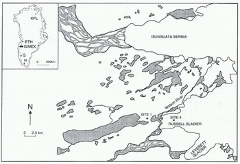
Fig. 1. Location of sites 1 and 4 during GIMEX. Dark-shaded areas represent lakes, light-shaded areas represent the ice surface. The inset shows same of the locations that are mentioned in the text: ETH, ETH camp; KCL, Kronprins Christians Land; N, Nordboglacier; Q, Qamanârssûp sermia. .Not included in the figure are Camp IV, which was located close to the ETH camp and the Free University of Amsterdam, located at 88 km from the ice edge in the GIMEX profile.
Ablation measurements were undertaken at three places in the close vicinity of site 4, and inter-stake variations for the period under consideration were typically less than 10 cm or 5% (Wal and others, in press). On a hill top just in front of the ice margin, a similar mast was erected (site 1, 300 m a.s.l.; Fig. 1), which should be more or less representative for free-atmosphere conditions at the same elevation as .site 4. Data from this mast will be used to estimate the inversion strength at site 4 in the section dealing with longwave radiation. Cloudiness (type and cover) was observed every 3 h.
Table 1 gives some average values at site 4 during GIMEX-91. The temperature at 2 m, T 2m, was continuously above the melting point. The wind is clearly of katabatic nature, blowing from the ice sheet with very high directional constancy dc and a typical speed V6in of 5 m s−1. Summer conditions in this part of Greenland are generally sunny and warm, with a mean cloud cover n = 0.5, resulting in high mean values of incoming .shortwave (Shw in) and longwave radiation (Lw in). The surface albedo α is relatively high for ice with 55%. A general description of the experiment has been given by Oerlemans and Vugts (1993). A more detailed description of the climate of the ablation zone can be found in Broeke and others, (1994a), Several papers on GIMEX have been published in a special issue of Global and Planetary Change (No. 9, 1994).
3. Global Radiation
Accuracy of the daily mean global-radiation measurements after recalibration is estimated to be typically better than 10 W m−2. Konzelmann and others (1994) presented a parameterization of the global radiation for the Greenland ice sheet as a function of several variables, of which the most important are date, elevation, cloud cover and surface albedo. In this method, no distinction is made between different cloud types but cloud transmission is made a function of elevation to account for the thinner clouds that are more frequently observed high above the ice sheet. Daily mean values of measured and parameterized global radiation during GIMEX-90 and 91 are given in Figure 2. Note that GIMEX-91 data are not independent, because they have been used to make the parameterization. However, the (independent) data collected during GIMEX-90 show a similarly satisfactory fit. The scatter increases for low values, which is caused by the strongly varying optical thickness of overcast skies, a factor that is not accounted for in the parameterization, Although the distance of the individual points to the 1: 1 line can be quite large (standard deviation of the GIMEX-90 daily means: 40 W m−2), the difference between the period means is acceptable, 8 W m−2 or 4%. If global radiation is measured, the inverse form of the parameterization can be used to calculate cloud amount n(0 < n < 1; Fig. 3). Difference between measured and calculated cloud amount for the GIMEX-90 data is only 2%, with a standard deviation of 14%, which is accurate enough for the calculation of the incoming longwave radiation (see next section). The results show that this kind of parameterization can also be used for the distinction between cloud rover and a snow surface for satellite pictures, i.e. to judge from automatic weatherstation data whether there is a cloud cover present or not in a certain area.
Table 1. Average characteristics at site 4 for the period 10 June-31 July 1991, bases on daily mean values; symbols are explained in the text.
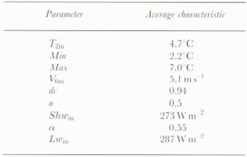
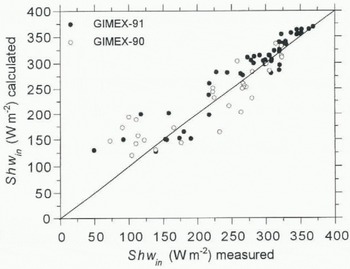
Fig. 2. Daily menu observed vs calculated global radiation. Shwin at site 4 for GIMEX-90 (open dots) and GIMEX-91 (solid dots). The Shwin calculation is according to the parameterization of Konzelmann and others (1994).
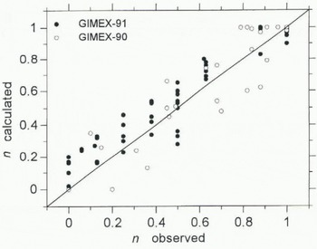
Fig. 3. Daily mean observed vs calculated cloud cover n at site 4 GIMEX-90 (open dots) and GIMEX-91 (solid dots). The calculation is according to the inverse parameterization of Konzelmann and others (1994).
4. Longwave Radiation
Longwave radiation was not measured directly but estimated by subtracting the global (shortwave) from the total radiation. This procedure, together with the typical measuring accuracy of the sensors, yields an estimated accuracy of the measured daily mean incoming longwave radiation Lw in of 15 W m−2. We compared the measurements with the results of two parameterizations for incoming longwave radiation: Konzelmann and others (1994) proposed a parameterization of Lw in for the Greenland ice sheet as a function of T 2m , water-vapour pressure e 2m and cloud amount n (Equation (1)), based on measurements undertaken at the ETH camp (69°34′ N, 1155 m a.s.l). König-Langlo and Augstein (1994) proposed a similar expression based on measurements undertaken at the polar stations Koldewey on Svalbard and Georg von Neumayer in Antarctica (Equation (2)), without inclusion of e 2m:

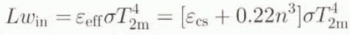
where ε eff , ε cs and ε oc . are the effective, clear-sky and overcast emissivity of the atmosphere, respectively, and σ the Stefan–Boltzmann constant. Figure 4 compares the measured and calculated Lw in for GIMEX-91. Between 260 and 300 W m−2, the calculated Lw in systematically underestimates the measured Lw in by 20–30 W m−2. This can be ascribed to the use of T 2m in Equations (1) and (2), which is not a reliable measure for the temperature of the lower atmosphere above a melting ice or snow surface. Due to the strong surface inversion, especially in the lower parts of the ice sheet, it will systematically yield too low values. The damping effect of the melting ice on the temperature near the surface is illustrated by the small range of daily mean T 2m during GIMEX-91 (5.5 K), while the measured values of Lw in during clear-sky conditions represent a range of clear-sky radiation temperature of 9.3 K. The systematic underestimation of Lwin for temperatures above freezing can also be traced back in the graphs on which the parameterizations on which Equations (1) and (2) are based, i.e. Figure 13 in Konzelmann and others (1994) and Figure 1 in König-Langlo and Augstein (1994). For higher values of Lw in (> 300 W m−2), strong large-scale winds effectively mix down the warm air, thereby decreasing the inversion strength. Under these conditions both parameterizations yield better results.
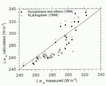
Fig. 4. Daily mean observed vs calculated incoming longwave radiation Lwin at site 4 during GIMEX-91. The Lwin calculation is according to the parameterization of Konzelmann and others (1994) (solid dots) and König-Langlo and Augstein (1994) (open dots).
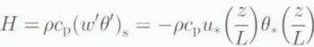
Figure 5 shows the effective emissivity ε eff averaged over intervals of cloud amount n. The differences between the two parameterizations are small, although the expression of Konzelmann and others (1994) yields slightly better results for high cloud amounts owing to the inclusion of ε oc in their expression. The error bars for the Konzelmann data arise from the inclusion of the water-vapour pressure in their parameterization. For strong inversion cases, ε eff is significantly too low in both expressions. Figure 6 shows the difference of Lw in between parameterization and measurements as a fund ion of temperature difference between sites 1 and 4. which can be regarded as a measure of the temperature inversion above the melting ice. It appears that an increasing inversion strength causes an increasing error in the calculated value of Lw in at an approximate rate of 10 W m−2 K−1 for both parameterizations. Especially, for ice bodies in warm environments, this could lead to serious errors in estimates of Lw in. In the case of GIMEX-91, the maximum error is 20–30 W m−2.
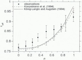
Fig. 5. Observed and calculated effective emissivity εeff vs cloud amount intervals n at site 4 dining GIMEX-91. The calculations are according to the parameterization of Konzelmann and others (1994) (dashed line) and König-Langlo and Augstein (1994) (solid line). Error bars in the curve of Konzelmann and others (1994) represent the standard deviation due to water-vapour pressure.
5. Turbulent Fluxes
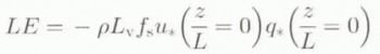
The turbulent fluxes of sensible and latent heat (H, LE) were calculated from mean variables measured at one level (6 m) and by assuming that the surface was melting, as described by Munro (1989). This method has the advantage that the surface values for temperature and moisture are well known and the differences between the levels are larger than between two levels in the atmosphere. The surface layer above a melting glacier is continuously stably stratified, so turbulence is suppressed by the stratification. To calculate the stability correction of the turbulent fluxes, we compared two different methods. The first method uses the well-known expressions according to Monin–Obukhov (M.O.) similarity theory (see, e.g., Duynkerke and Broeke, 1994):
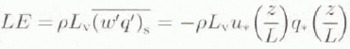
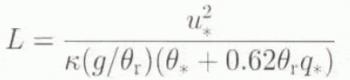
where ρ is the air density, c p is the Specific heal of air at constant pressure, L v is the latent heat of vaporisation, z is the measurement height, L is the Monin–Obukhov length, w′, θ′ and q′ are the turbulent fluctuations of wind, temperature and humidity, and u * , θ * and q * are the associated turbulent scales, which are functions of the dimensionless stability parameter zL −1. is the von Kármán constant, g is the acceleration of gravity and θ r . is a reference temperature. The stability functions are taken from Duynkerke (1991) and will not be given here. Because zL −1 in its turn depends on the surface fluxes, this calculation method requires an iterative procedure (implicit method).
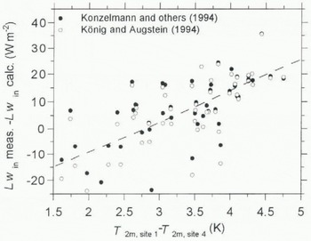
Fig. 6. Difference between measured and calculated mean Lwin at site 4 vs potential temperature difference between sites 1 and 4 during GIMEX-91, according to the parameterization of Konzelmann and others (1994) (solid dots) and König-Langlo and Augstein (1994) (open dots). The temperature difference is assumed to be a measure of the surface inversion at site 4.
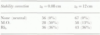
Table 2. Average sensible-heat flux H (W m −2 ) for the period 15 June–31 July 1991. Stability corrections are discussed in the text. Percentage between brackets is the redaction of H when compared to the neutral (uncorrected) value
Secondly, we will try a simpler, explicit stability correction originally proposed by Louis (1979). This expression is often used in meteorological models for its computational efficiency (Greuell and Konzelmann, 1994; Meesters and others, 1994). The fluxes for the neutral case (zL −1 = 0) are multiplied by a factor f s that accounts for stability effects (0 < f s < 1 for stable conditions):

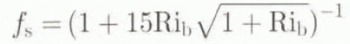
where Rib is the bulk Richardson number, that can be calculated explicitly from the measurements:
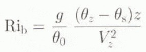
in which V is the wind speed and the subscript s refers to the surface values. This method will be referred to as the “Rib correction”.
For both methods, we still must specify at which height the profiles of wind, temperature and moisture attain their surface values. At z = Z 0, the surface-roughness length for momentum, the wind speed extrapolates to zero. The roughness length for heat and moisture z h , is a function of the flow and can be calculated using the expression developed by Andreas (1987) that expresses z h as a function of the roughness Reynolds number, Re = u* z 0 v −1, where v is the kinematic viscosity of air and u* is the friction velocity, We tried two different values of z 0: a value obtained from wind profiles (z 0 = 0.08 cm; Duynkerke and Broeke, 1994) and one obtained from microtopographical survey (z 0 = 12 cm) according to the method described by Lettau (1969). The results for the sensible-heat flux H during GIMEX-91 are summarized in Table 2; the average latent-heat flux LE was negligibly small for all experiments (< 1 W m−2) and is not shown here.
The Rib, stability correction assumes a typical value of the surface roughness (lower than is encountered at site 4) and reduces the “neutral” flux by 36%. Tins appears to be an unjustified simplification, given the very different results obtained with the physically more realistic M.O. theory. This can be understood as follows: in the stable surface layer, turbulence is generated mainly by wind shear which, of course, strongly depends on the surface roughness. Consequently, the explicit method overestimates the flux reduction above a rough surface in stable conditions, leading to underestimation of the turbulent fluxes.
6. Effects of the use of different para-meterizations on the calculated amount of melt
The energy balance above a melting ice surface can be written as:
where M is the melting energy. In all subsequent calculations we have neglected the contribution of the sub-surface heat flux, G, i.e. the sub-surface layers tire assumed to be isothermal at 0°C. This assumption is justified for the lower ablation zone in the high summer (Ambach, 1977). Using some of the parameterizations and assumptions discussed in the previous sections, we calculated the melt M and compared it to the measured ablation, Figure 7 shows the calculated and observed amount of melt for the period 15 June–31 July 1991, based on the use of the different parameterizations, The error bars for the ablation measurements represent the typical 5 cm standard deviation of the ablation measurements between the three slakes. Figure 7 shows that the measured ablation of 2070 mm w.e. is predicted accurately within 2% (upper line) if we use the measured values of Shw in and Lw in , the value of z 0 obtained by microtopographical survey (12 cm) and the stability correction according to M.O. similarity theory. Using the parameterization (1) to calculate Lw in and assuming a melting surface to calculate Lw out yields a shortage of melting energy of 16%. Use of the explicit stability correction to calculate the turbulent fluxes results in a 9% energy shortage. Using Z 0 as determined from profiles (Z 0 = 0.08 cm) underestimates the melting energy by 18%. All these deviations are well outside the uncertainty of the ablation measurements and work in the same direction, which excludes the possibility of error cancellation. As was stated in section 3, the use of a parameterization for global incoming radiation yields good results for this data set.
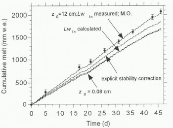
Fig. 7. Calculated (lines) and observed (solid dots) cumulative melt (mm w.e.) at site 4 during GIMEX-91, based on hourly mean values. Error bars represent typical standard deviation of the ablation measurements. .Vote the clear daily cycle in the calculated melt curves, which is due to the pronounced daily cycle in the melting energy.
Figure 8 shows the distribution of the different terms in the energy balance, based on calculations represented by the upper curve in Figure 7. Melting is mainly caused by net shortwave radiation (2/3) and the sensible-heat flux (1/3). These results agree qualitatively with the energy-balance distribution at Qamanârssûp sermia, near Nuuk (Godthåb), at 790 m a.s.l. (Braithwaite and Olesen, 1990). The quite large contribution of H to the energy balance (58 W m−2) can be ascribed to the large aerodynamic roughness of the surface and the persistent katabatic winds. This shows that surface melting in the lower parts of the Greenland ice sheet is probably sensitive to variations in ambient temperature and katabatic wind speed. In this context, it is interesting to note that underestimation of H in meteorological models causes an underestimation of the katabatic wind speed, since this wind is primarily forced by the surface cooling flue to the sensible-heat flux (Broeke and others, 1994b). In this study, the contribution of the latent-heat flux LE is very small. It is interesting to note that evaporation (negative latent-heat flux) is generally an important term in the higher ablation zone (Ambach, 1977; Greuell and Konzelmann, 1994; Henneken and others, 1994). Numerical modelling of the energy balance shows that downslope advection of moisture by the katabatic wind forces this term to become small, or even reversed in the lower ablation zone (Broeke, in press).
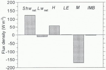
Fig. 8. Energy balance at site 4 during GIMEX-91, based on the upper curve in Figure 7. IMB represents the imbalance between measured and calculated melting energy (3 W m−2 or 2%)
7. Conclusions
In this paper we presented the energy-balance distribution at a site in the lower melting zone (340 m a.s.l.) of the West Greenland ice sheet in summer, based on 86 daily mean observations during GIMEX-90 and 91. The summer climate at this site is warm, dry and sunny, with a seasonal ablation rate of 3.1 m w.e. Melting is primarily caused by net radiation (2/3) and the turbulent flux of sensible heat (1/3). The relatively large contribution of the sensible-heat flux (e.g. when compared to mid-latitude valley glaciers) can be ascribed to the high albedo, the large aerodynamic roughness and the persistent katabatic winds.
We compared the observations with various parameterizations that are currently used in meteorological and glaciological models. Provided that one knows the surface albedo, the net shortwave radiation can be estimated from cloud cover and surface elevation with sufficient accuracy, using the parameterization presented by Konzelmann and others (1994). On the other hand, if the global radiation is measured, a good estimate of cloudiness can be made using the inverse parameterization. These values are accurate enough to use in longwave radiation calculations or to determine cloud amount as ground truth for satellites. The temperature at 2 m is no longer an accurate estimate of the temperature of the lower atmosphere when a strong temperature inversion is present above the melting ice, which is the case for the lower ablation zone. As a result, the two parameterizations that were tested in this study underestimated LW in by as much as 28 W m−2. The parameterization by Konzelmann and others (1994) yields slightly better results in the limit of cloud-covered skies through the inclusion of an effective emissivity for overcast conditions. The parameterizations work well higher up on the ice sheet, where the surface inversion is weaker (Konzelmann and others, 1994).
Two stability corrections, as well as two different values of Z 0, have been tested to calculate the turbulent fluxes of sensible and latent heat. The observed melt was calculated well if we used the value of Z 0 obtained by microtopographical survey of the terrain (Z 0 = 12 cm). The value obtained by profile measurements (Z 0 = 0.08 cm) appears to be erroneously small. The explicit stability correction proposed by Louis (1979) underestimates the sensible-heat flux on average by 26%. The turbulent fluxes of latent heat LE were very small in all experiments (< 1 W m−2). Note that underestimation of H in meteorological models causes an underestimation of the katabatic wind speed, since this wind is primarily forced by the surface cooling due to the sensible-heat flux.
Acknowledgements
R. S.W. van de Wal and two reviewers are thanked for very useful comments on an earlier version of the paper. Financial support for this work was provided by the Dutch National Research Programme on Global Air Pollution and Climate Change (NOP).


