


The transfer of heat, water vapour and momentum between the atmosphere and the ground govern many of the physical processes enacted at the Earth’s surface. The rate of diffusion of properties of the atmosphere by means of turbulence at the Earth’s boundary layer is expressed by transfer coefficients. If there is a certain identity in the vertical profiles of these properties, the transfer coefficients for heat, for water vapour and for momentum arc assumed equal, the last being evaluated from measurement of the variation of wind speed with height. The form of the vertical profile of wind speed depends upon the physical characteristics of the surface and the stability in the atmosphere over it. Air stability is expressed as a ratio of the buoyancy forces to the inertial forces and may become so strongly positive that wind eddies are suppressed near the surface—say in the lowest one or two metres of air. Something near to this condition is experienced frequently over a melting ice surface which thus offers an ideal opportunity for measurement of the range of turbulent mixing to correlate with stability and hence find the exchange coefficients.
With the inherent difficulties of subjecting meteorological conditions to laboratory techniques, most of the equations postulated as expressing the increase of wind speed with height, have arisen empirically. Essentially, a universal law is sought which is applicable throughout the range of stabilities normally experienced in the surface layer of the atmosphere; the law should not be so complex that it is generally impracticable. This paper considers the laws of wind-speed variation with height in relation to available detailed measurements of wind speed and temperature in the lowest 2 m. over various snow and ice surfaces.
Notation
The following symbols and abbreviations are used:
-
a, c constants for specific ranges of stability
-
B inverse of a stability length =

-
Cp specific heat of air at constant pressure
-
f(n) function of n
-
g acceleration due to gravity (cm. sec.−2)
-
H turbulent heat flux =
-
k von Kármán’s constant 3≈0.4
-
K M eddy coefficient of momentum (eddy viscosity) (cm.2 sec.−1)
-
K M * dimensionless eddy viscosity =
-
K H eddy coefficient of heat (eddy conductivity) (cm.2 sec.−1)
-
l mixing length
-
l 1 mixing length at height z 1
-
L
-
L′
-
n power parameter >1
-
p power parameter
-
r linear dimension of object, e.g. radius of sphere in fluid or of pipe carrying the fluid (cm.)
-
Re
-
Ri
-
Rif
-
Riz Richardson number at height z
-
s standard height (cm.)
-
S
-
T air temperature (°K.)
-
T 0 mean temperature (°K.)
-
u *
-
u z wind speed (cm. sec.−1) at height z (cm.)
-
u′, w′ eddy components of wind speed, parallel with, and perpendicular to, the mean flow (cm. sec.−1)
-
υ velocity of fluid (cm. sec.−1)
-
X non-linear height variable = L[exp(z/L)−1] (cm.)
-
z 0 surface roughness parameter (cm.)
-
α, γ, y′ constants for specific ranges of stability
-
β
-
Γ dry adiabatic lapse rate (≈+1 × 10⁻⁴ °C. cm.−1)
-
δ measured deviation from the logarithmic law (cm. sec.−1)
-
Δ
-
λ
-
v molecular (kinematic) viscosity (cm.2 sec.−1)
-
ρ density of air (g. cm.−3)
-
σ standard deviation of z 0 (cm.)
-
τ the eddy flux of momentum or shearing stress (g. cm.−1 sec.−2)
-
τ 0 shearing stress at the ground (g. cm.−1 sec.−2)


I Review of Existing Laws
(a) The logarithmic law
Experiments with fluids of uniform density distribution, in pipes and over flat plates, indicate that the velocity varies as the logarithm of the distance from the boundary. This relationship is applicable over smooth or rough surfaces with turbulent flow, which may be recognized by fairly high Reynolds numbers (Re > 75 × 105). For the atmosphere, there is no adequate definition of the characteristic length required by the Reynolds number but turbulent flow prevails. In a neutral atmosphere, i.e. when the vertical profile of air temperature is governed only by change in pressure, the vertical wind profile appears to follow a logarithmic distribution. Many observers have found that the logarithmic law is applicable over a fairly wide stability range (Reference BruntBrunt, 1939, p. 247), but becomes less satisfactory (Fig. 1) as stabilities depart from neutral (Reference PasquillPasquill, 1949[a], p. 124).

Fig. 1. Effect of stability on the variation of wind speed with height
The mixing-length hypothesis, though somewhat discredited, has not been replaced by any very satisfactory approach. That hypothesis postulates that l is a unique length which characterizes the local intensity of turbulent mixing (Reference SuttonSutton, 1953, p. 73). Fundamentally the logarithmic law rests on the assumption that velocity fluctuations in both vertical and horizontal directions are identically proportional to the wind-speed gradient, i.e.

The shear stress

With the supposition that l varies linearly with height (l = kz)

The constant introduced on integration is a measure of the surface roughness, being the height (z 0) at which the wind speed is zero and hence incorporated in the logarithmic law generally expressed as

and, since the wind shear

the eddy viscosity

(b) Power laws
A less exact expression has been evolved, similarly from pipe flow, relating velocity with a fractional power of the distance from the boundary. The power parameter may be modified to extend the applicability of the law through the whole range of stability. Since this power reflects surface roughness also, it is not an independent index of stability. Over grassland, the power varies from


therefore

This simple power law is not now used since it does not incorporate the friction velocity u * nor the surface roughness parameter z 0 and the power index can be most unsatisfactory. To overcome these difficulties Deacon advanced empirically, a systematic power parameter which would account for observed deviations from the logarithmic law in non-neutral stability and be applicable to all stability ranges (Reference DeaconDeacon, 1949). In addition, the power is independent of surface roughness.
The velocity profile is represented by

where β > 1 in unstable conditions, β<1 in stable conditions, and β = 1 in neutral stability when the expression reduces to the logarithmic law. The eddy viscosity becomes

Priestley states (Reference Priestley1959, p. 30) that Deacon’s law is the simplest and most widely used; Reference DalrympleDalrymple and others (1963, p. 13) applied Deacon’s law to analysis of micro-meteorological data at the South Pole; this power law is, however, not satisfactory for a very stable atmosphere.
(c) Logarithmic-plus-linear laws
Holzman and earlier workers such as Rossby and Montgomery (Reference SuttonSutton, 1953, p. 265) suggested incorporating a function of stability into the logarithmic law. Reference Monin and ObukhovMonin and Obukhov (1954, p. 6 of translation) added a function of height and stability for the deviation from the logarithmic form;

The function F was expanded as a simple power series in terms of z/L and the first two terms used

Stability is expressed as the ratio of wind shear, represented by the momentum flux, to the buoyancy forces represented by the heat flux and opposed by gravity. The Richardson number (see notation) is generally used as a parameter of stability but since this involves drawing tangents to vertical profiles of temperature and of wind speed, simpler expressions are frequently adopted. Monin and Obukhov expressed stability as

which gives dimensions of inverse length. For use in the wind-speed expression, by combining all the appropriate elements of the flux equations:
the wind shear

the heat flux

and
Monin and Obukhov found a stability length

This was used in the wind-profile equation from (8)

which produces an eddy viscosity

These expressions assume, from the apparent similarity of the temperature and wind-speed profiles, that the exchange coefficients for heat and momentum, if not identical, vary with height at a constant rate, i.e. K H /K M = constant. Without actual heat flux measurements, the characteristic stability length L and the universal constant α may be found only by regression involving the modified Richardson number, B. Assuming that temperature can also be expressed similarly to (10) then

where

and α/L can be determined from three wind speeds using equation (10). Monin and Obukhov, using data from more than 800 profiles, through a stability range, indicated by B, from −0.084 to 0.015, found α = +0.62. They suggest other functions might be more suitable outside a moderate stability range. Recently Reference TaylorTaylor (1960, p. 77) found that different constants for various stability regimes are more suitable as indicated by Table I. In conditions of free convection (temperature lapse), which are infrequent over melting ice surfaces, Taylor considers that this logarithmic-plus-linear law does not apply.
Table I. Values Derived from Observations over Grassland of the Logarithmic-plus-Linear Law constant α
(after Reference TaylorTaylor, 1960, p. 77; Reference DeaconDeacon, 1962, p. 3171; Reference Monin and ObukhovMonin and Obukhov, 1954, p. 20).

Reference EllisonEllison (1957, p. 461) employs a modified form of the momentum coefficient

from equations (1) and (3)

to determine the function


approximates to a logarithmic-plus-linear law

where

Using Rider’s data, Ellison finds α = 0.8 which compares with α = 0.6 by Monin and Ohukhov. To overcome the lack of absolute measurement of fluxes, Reference PanofskyPanofsky and others (1960, p. 390) suggest

and

Expression (14) becomes

and the eddy viscosity

The stability length L′ associated with this variation of the logarithmic-plus-linear Iaw may be defined in terms of actual gradients of wind speed and temperature. This avoids dependence on stability indices or actual heat-flux measurements, but places heavy reliance on the graphical construction of the profiles. Observational data appear to indicate a constant γ′ = 18 for all except very stable conditions (Reference PanofskyPanofsky and others, 1960, p. 393). In such conditions, Panofsky and others suggest that factors not considered in the similarity theory may become important. Reference YamamotoYamamoto (1959, p. 68) using Rider’s data over short grassland, found γ′ = +56 in unstable and neutral conditions and, less distinctively, γ′ = +7.3 in a stable atmosphere.
An equation of similar logarithmic-plus-linear form has been suggested to account for deviations of wind speed from its variation with the logarithm of height, especially in inversion conditions (Reference LiljequistLiljequist, 1957, p. 212). However, as Liljequist suggests, a large vertical range of observational data (up to 10 m.) is required for the definite recognition of the deviation; it is scarcely possible for observations limited to the lowest 2 metres.
(d) Exponential law
To account for the change of shape of the wind profiles as indicated in Figure 1, Reference SwinbankSwinbank (1964, p. 120) introduces into the form of the wind velocity gradient at neutral stability

a variable X which should be a function of heat and momentum fluxes as well as height

Swinbank expresses the kinetic energy of turbulence in terms of the shearing stress and the buoyancy

from which the non-linear height X is evolved in terms of L

The wind gradient then becomes

from which the difference between two wind speeds

With a value for k and wind-speed observations at three heights, the length L and the friction velocity u * can be evaluated.
Reference SwinbankSwinbank (1964, p. 123) shows that small errors in k (generally taken as = 0.4) can be significant. Errors in u * will be equally significant; so to avoid these the measurements at three heights are expressed as

Although Swinbank’s exponential expression does not propose any critical value of stability, it transforms to the logarithmic law in slight stabilities.
From (17)
II Apparatus
For the observations analysed here, the following apparatus was used:
Cassella-Sheppard sensitive cup anemometers were set up at all the sites. On the Britannia Gletscher, Greenland, they were mounted at 30, 100, 200 and 400 cm.; on Britannia Sø, Greenland, at 6, 10, 30, 100 and 200 cm.; in the Tarfala valley, Sweden, at 10, 30, 100, 200 cm. and on the Storglaciären, Sweden, at 100 and 200 cm. These last, giving the wind run over a half or one hour interval, were a control on mean values of instantaneous wind speeds read successively from hot bulb anemometers mounted at 1, 2, 4, 6, 8, 12, 30, 100 and 200 cm. The hot bulb anemometer had been made to reduce the size of the anemometer and obviate errors probable in closely setting the instruments, particularly near the surfaces, for detailed vertical profiles. It comprised a sensistor (a semi-conductor with a high temperature coefficient of resistance) heated by a constant voltage across it and cooled by the air flow, which varied the temperature and hence the bulb resistance, which was in turn measured by amplifying the out-of-balance current of a Wheatstone bridge. For reduction of rapid fluctuations and part protection from the weather, the bulb was mounted vertically at the centre of a fine wire gauze cylinder (Reference CaisleyCaisley and others, 1963, p. 42).
In Greenland and at the valley station in Sweden, thermocouples were used to measure profiles of temperature and vapour pressure (Reference Lister and TaylorLister and Taylor, 1961, p. 10). The apparatus was similar to that of Reference PasquillPasquill (1949[b], p. 239). The 28 s.w.g. copper/constantan thermocouples were set in
On Storglaciären, temperature and humidity profiles were measured by resistance thermometers (sensistors), mounted as wet and dry bulbs along a single axis of concentric radiation screens and a small 12 V. motor and fan for aspiration (Reference CaisleyCaisley and others, 1963, p. 39). Fine copper wire was wrapped around each sensistor to lag the response to temperature and humidity changes. Resistance values were obtained with the same Wheatstone bridge used to measure wind speeds. At each of the Storgtaciären sites, nine of these compact units were mounted at 1, 2, 4, 6, 8, 12, 30, 100 and 200 cm.
Mean profiles of wet- and dry-bulb temperatures were taken from at least six sets of profiles read at approximately equal intervals through one hour. Observations were made during alternate hours for periods varying from 8 to 48 hr. on various days in the ablation season at each glacier.
Instruments were interchanged vertically along their respective masts to ensure that any experimental error would not systematically affect the whole series of observations.
Accuracy of the cup anemometers has been given as 2 cm. sec.−1 but on a glacier, verticality of the spindle cannot be perfectly maintained so ±5 cm. sec.−1 is more realistic. The hot-bulb anemometers, calibrated in a wind tunnel, had an accuracy of ±8 cm. sec.−1; the thermocouples ±0.05°C.; the temperature measuring sensistors ±0.04°C. The sensistors were found, by recalibration, to have remained stable throughout the period of the field work. Error in height interval between instruments was not more than 0.5 cm. but the coincidence of the height zero with a mean surface was inevitably the most difficult to achieve in the field. From the plotted data, however, the height datum does not seem to be in error by more than ±1 cm. These errors were not exceeded when drawing vertical profiles, values from which were used in calculations.
III Sites where Observations were Recorded
Wind-speed and temperature measurements recorded during the melting season were used from the following sites (the designation numbers are retained in Fig. 2):
-
Tarfala valley, 3.5 km. long, 0.5 km. wide across the bottom of the U-shaped cross-section, runs approx. north-south in the Kebnekaise massif in north Sweden. This hanging valley has three tributary valleys occupied by glaciers, though the main valley is snow-free in summer; it is steep walled and floored by fluvially re-worked moraine with sparse, very short vegetation. The site of observation was on a gentle slope averaging 4 degrees that increased to the east, into the valley wall. Stone fragments and cobbles, interspersed with patches of thin soil and moss were dotted irregularly with 20 to 50 cm. dia, boulders. These last were cleared from the immediate location of the site and were sparse in the direction of the prevailing wind, down-valley.
cm. with standard deviation σ = 0.12 cm. Station height 1,110 m. lat. 67° 53′ N., long. 18° 38′ E. -
Storglaciären, 3 km. long, 0.8 km. wide, flowing east from the cliff slopes of Kebnekaise, in one of the valleys mentioned above. Two stations were set up approximately on the centre line of the glacier surface which had a 4 to 5 degree slope and was snow-covered initially but changed to coarse firn and then largely to smooth ice intersected in places by melt-water channels. Wind over the surface was generally at a small angle to the centre line and more frequently down-glacier.
cm. σ = 0.002 cm. Upper Station: height 1,385 m., lat. 67° 53′ N., long. 18° 35′ E. Lower station: height 1,325 m., lat. 67° 53′ N., long. 18° 36′ E. Since these stations were 1 km. apart with similar surfaces the observations are taken in one group in Figure 2. -
Britannia Sø, approximately 10 km. long, 3 km. wide, is a frozen, ice-dammed lake in north Dronning Louise Land, north-east Greenland. Instruments were sited 200 m. from the northern shore of the lake and operated when the wind was east or west, giving a fetch of approximately 2 km. over the melting ice surface, which had slightly roughened patches where the ice had candled.
cm. σ = 0.005 cm. Station height 223 m., lat. 77° 09′ N., long. 23° 40′ W. -
Britannia Gletscher, 14 km. long, 8 km. wide, is a valley glacier flowing south into Dronning Louise Land from the Greenland Ice Sheet. Above the comparatively steep glacier snout, overall slope varied little from 2 degrees. Coarse snow in sastrugi 10–40 cm. high at the beginning of the melt season gave place to undulating wet snow and finally to bare, hum-mocked ice. The upper station data is representative of conditions on the margin of the inland ice. Apparatus was located 1.5 km. from the eastern edge of the glacier but the wind, largely N.N.W., had a fairly uniform fetch of nearly 4 km.
cm. (early summer z 0 = 1.1±0.25, middle summer z 0 = 0.68±0.14, late summer z 0 = 0.58±0.15). Upper Station: height 620 m., lat. 77° 14′ N., long. 23° 48′ W. -
Britannia Gletscher, the lower station data are representative of conditions over the ablation zone of the glacier. The station was 0.5 km. from the glacier edge but well clear of changes in slope and steeper streams, though towards the end of the ablation season, a deep channel passed near the site. The surface was fairly uniform over 5 km. upwind.
cm. (early summer z 0 = 0.40±0.16, middle summer z 0 = 0.50±0.31, late summer±0.15). Lower station: height 460 m., lat. 77° 12′ N., long. 23° 48′ W.

Fig. 2. Mean deviation of wind speeds (observed in the lowest 2 m.) from laws of wind-speed variation with height. The two scales on the ordinates are “goodness of fit” 0 to 1 and mean deviation expressed as a percentage of the mean wind speed at 1 m. The abscissa scale gives the number of vertical wind profiles for which the respective law was applicable and is divided into groups for different sites; the dotted line gives the mean fit for all sites. The summary on the right indicates the applicability of each law at all stabilities
IV Application of Existing Laws to Observed Data
As a first step in finding the coefficient of eddy diffusion for subsequent evaluation of heat and vapour transfer over the various melting ice surfaces, the observed wind-speed profiles were examined to find which law of wind-speed variation with height offered the best fit. When classified into stability groups according to the Richardson number the data confirmed first impressions that unstable conditions were infrequent over melting ice. Highest stabilities (Ri > +0.5) were found on the Britannia Gletscher, especially at the lower station where low wind speeds (
(a) Suitability of the logarithmic law
The logarithmic law was most applicable in neutral conditions and, very unexpectedly, in marked inversions also (an example is shown in Figure 3). For each site the surface roughness parameter was evaluated from this law in neutral conditions and has been given with the site descriptions in section III. Roughness parameters of the same order of magnitude have been determined by other workers at similar sites (e.g. Reference SverdrupSverdrup, 1936; Reference LiljequistLiljequist, 1957; Reference KeelerKeeler, 1964). The friction velocity, u *, was usually within the range 45 to 15 cm. sec.−1.

Fig. 3. Wind profiles and associated temperature profiles in various stabilities at the lower glacier site on Britannia Gletscher
(b) Suitability of the power laws
A power law, and Deacon’s modification of it, also fitted the observations fairly well, but, within stability groups, the variation of the power parameters was often quite large as shown in Table II and Figure 4. On the frozen lake and at the Swedish sites, the index 1/n for the power law in neutral conditions was approximately

Fig. 4. Variation with stability of the index n in Sverdrup’s power law (expression (4))
Table II. Variation with Stability of Constants in Laws of Wind-Speed Variation with Height Figures in brackets indicate number of profiles used here.
Sites: 1 Ice-free surface (Tarfala valley)
2 Storglaciären
3 Frozen lake (Britannia Sø)
4 Britannia Gletscher—upper
5 Britannia Gletscher—lower

Table III. The differences between Mean Estimates for Wind Speeds (cm. Sec.−1) by the Exponential Expression and that by All Other Laws
+ indicates that the exponential expression is superior, being nearer the observed value.

The β value in Deacon’s power law (Table II and Fig. 5) was generally greater than unity even in stable conditions. A minimum is suggested for β in Figure 5 at what appears to be a critical value of Ri = 0.2. It seems that neither the logarithmic nor the power laws are satisfactory through the range of stability experienced over melting ice.
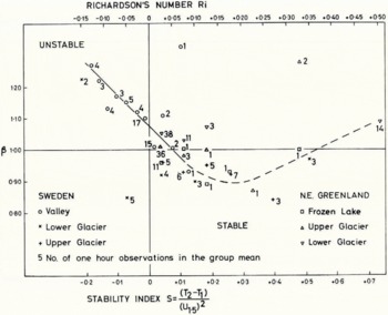
Fig. 5. Variation with stability of the index β in Deacon’s power law (expression (6))
(c) Suitability of the logarithmic-plus-linear laws
Following Monin and Obukhov’s theory, different constants were derived for various stabilities at the six sites. Figure 6 shows the regression between B and f (α/L) for the ice-free valley site. From Table II it appears that α (in expression 10) is not a universal constant. Table II shows a variety of constants evaluated for the second logarithmic-plus-linear law (15). At very great stabilities Ri > +0.5 a relevant constant could not be distinguished and generally this law gave a relatively poor fit. The main difference between these two laws is that for Monin and Obukhov’s law the ratio α/L is found from each profile and this ratio determines the remaining velocities at various heights for comparison with observed wind speeds. For the second log-plus-linear law, however, each profile gives z/ L′ (after Reference PanofskyPanofsky and others, 1960), but γ′ must be found graphically from Ellison’s relationship between K/K M * and z/ L′. The applicability of the first law to each profile, is, therefore, independent of a general constant, although this is essential to the second law. Hence the first logarithmic-pluslinear law would be expected to fit individually, better than the second law, as it appears here (Fig. 2).

Fig. 6. Variation with stability B of constants in Monin & Obukhov’s logarithmic-plus-linear law (expression (10)). Data from the ice-free Tarfala valley
(d) Suitability of the exponential law
To apply Swinbank’s exponential wind profile (18) directly to the observations, Figure 7 was prepared giving the ratios of wind-speed differences for various values of L. Similarly the friction velocities were derived as a function of L. From Figure 7 it will be seen that there is a limiting wind ratio for the depth of the air layer concerned. As L increases in neutral stabilities, the extreme ratio of expression (18) becomes


Fig. 7. Variation of L with the ratio of wind-speed differences in Swinbank’s exponential law
With z 1, z 2, and z 3 = 30, 50 and 100 cm. this ratio is 2.36. Ratios beyond this limit were found to have occurred for some of the inversion conditions but for 38 per cent of the wind profiles, a stability index L and a friction velocity u * could be determined. With these values, the velocities at 200 cm. and 10 cm. have been calculated to compare with observed wind speeds at these heights. The mean deviation for all sites considered range from 10.2 cm. sec.−1 over 21 profiles in adiabatic conditions to 3.2 cm. sec.−1 over 10 profiles in conditions of strong inversion.
The limit in the number of wind profiles to which the exponential law could be applied precludes a comparison of the fit of the law in the manner used in Figure 2 for comparison of other laws. But the differences between the total mean deviations of the exponential application and of the total mean deviations of the other expressions tried here, are shown in Table III.
Swinbank’s expression is more fitting over the whole stability range than the second loglinear law only, but for all lapse conditions it is the superior expression. There are few profiles in stable conditions to which the exponential form could be applied, but the differences resulting between it and the logarithmic law are very small.
Since fluxes were not available to accompany the wind-speed observations used here, L and u * could not be found independently for comparison with values determined from the exponential function. However, Reference SwinbankSwinbank (1964, p. 133) used a drag coefficient and wind speeds at low heights to estimate friction velocities and found a very high correlation (0.99) these with the values derived from his exponential expression; the observations were recorded in convection conditions. From the data in adiabatic and stable conditions analysed here, friction velocities were obtained using the exponential expression for the air layer from 10 to 100 cm. to give the most representative values for each wind profile. These were compared with friction velocities determined from the drag coefficient and wind speeds at 30 cm. (Fig. 8). The correlation coefficient for the III values found by the two methods is 0.56 with a significance level greater than 0.001. This comparatively low coefficient is indicated in Figure 8 by the wide scatter about the unit-gradient line. Generally, the estimates via the exponential function are too low.

Fig. 8. Comparison of u * found from the exponential law and from the drag coefficient
Thus, though Swinbank’s expressions seem more applicable than any other in lapse conditions, it does not satisfy the observations in a neutral nor in a stable atmosphere. The exponential expression implies a continuously increasing deviation of the wind-speed profile from the logarithmic form as stability intensifies. For the observations considered here, the logarithmic law is satisfactory in neutral and in high stabilities, so here the failure of the exponential law is apparent.
It must be concluded that none of the existing laws are satisfactory. The most difficult part of the range is in the stable region, which is dominant over melting ice. It is thus necessary to look further for one functional expression which would encompass the whole spectrum of stability conditions.
V Variation of the Richardson Number with Height
A problem arising from any form of velocity gradient as a function of the stability gradient is that of integration from the gradient expression to the wind-speed equation when the Richardson number is involved. Priestley (1959, p. 25) assumed that the Richardson number varies linearly with height. Reference DeaconDeacon (1953, p. 45) similarly suggested that a linear relation would be a good approximation since if

then

The power indices are a little different from unity and they do not change by the same amount under different stabilities, so the relation between stability and height though approximately linear may in fact be more complex. No systematic relationship between λ and β, or λ and stability was apparent in these observations, so Deacon’s expression for the Richardson number could not be employed.
The Richardson number itself can be found rather inaccurately, without an exact mathematical knowledge of the velocity and temperature profiles, by measuring gradients graphically.
As a stability index, only one value of the Richardson number is generally found for a profile, so little data on its variation with height are directly available. However, the Richardson number has been evaluated at 10, 30 and 100 cm. for 36 per cent (60 profiles) of the data used here. After grouping into classes, a distinctive pattern can be seen (Fig. 9) in which stability varies as a power of height and the power varies with the mean stability of the profile. If Ris and Riz are the Richardson numbers at a standard height and at height z respectively, then


Fig. 9. Variation of Richardson number with height z
This equation ensures a dimensionally correct function. For all the profiles observed over a 2 m. height interval, the Richardson number had been found at the mean logarithmic height of 55 cm. so Ri s became Ri55.
From Figure 9 it can be seen that as stabilities increase, gradients decrease until at

Hence

It may be noted that this expression implies that with Ri s = 0.2 stability is constant with height; below this value the power index is positive, Ri increasing with height. To accommodate temperature lapse conditions, in which Ri is negative a modulus sign is necessary, hence vert;Ri55vert; in the power index.
Though there is very little data on the variation of stability with height, Dalrymple’s observations at the South Pole give Richardson numbers at 1, 2, and 4 m. calculated from differences of observed values rather than from drawn gradients (Reference DeaconDalrymple, and others, 1964, p. 12). The form of the Richardson number used is

Using the Richardson number obtained at 100 cm. as a standard value, the Richardson number at 200 cm. has been calculated via the power function (21) and the linear function

The agreement of the calculated with the “observed” Richardson numbers is not very good but the agreement using the power function is slightly superior (Fig. 10). The root-meansquare of the deviations using the power function is 0.013 whereas that of the linear function estimate is 0.025.

Fig. 10. Comparison of observed and calculated Ri200 based upon Reference DalrympleDalrymple and others’ (1963) South Pole data
Independent of the characteristic stability of a profile, neutral stability predominates very near the ground. The function suggested here gives this relationship, but does not always indicate an increase of the Richardson number with height. For values greater than Ri s = 0.2 the maximum value of Ri must be found at heights less than the standard height. The power function of the variation of Richardson number with height is used in the subsequent analysis of wind-speed profiles.
VI Deviation of Wind Speed from the Logarithmic Form as a Function of the Richardson Number
In conditions of free convection, the mixing length (see Section I(a)) should tend to plus infinity and become zero at some high positive stability where turbulence is precluded. But the deviation from the logarithmic law for these observations over snow and ice has been shown (Fig. 2) to become a minimum at two separate ranges of stability. A cubic form thus seems appropriate (Fig. 11) for the relation of stability to the mixing length and, by differentiation, also for the velocity profile.
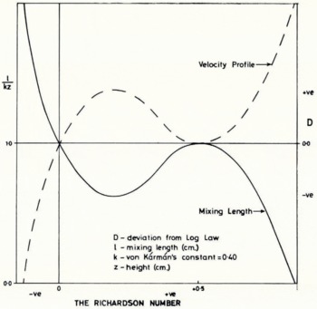
Fig. 11. Variation with stability of the mixing length and of the deviation of observed wind profiles from the logarithmic law, implied in Figure 2
The average deviation between observed wind speeds and those velocities determined from the best-fitting logarithmic expression was found for each profile (Section IV). The wind-speed deviation from the logarithmic form may be taken as positive in stable, and negative in unstable, atmospheres (similar to Figure I) and may be expressed, for all z, as

The cubic variation of δ with the standard Richardson number is apparent in Figure 12 although it must be noted that dimensionally, δ is a wind speed. To be pliable differentially, a simpler, dimensionless function is required, such as


Fig. 12. Variation with stability of the mean deviation δ in m.sec.−1 of observed wind-speed values from the logarithmic law
The same logarithmic profiles as used to find δ also gave u * This used the mean of the wind-speed observations near the surface but assumed the logarithmic distribution applicable. As a check on this, the u * values were also derived from the wind speed at the lowest height of observation and the drag coefficient u * 2/u 2 at that height, assumed to be the same as that found from near-neutral profiles. Figure 13 shows good agreement in most of the values of u * found by these methods. A cubic form of the variation of Δ with stability seems to be required as in Figure 14. A simple linear addition to the logarithmic law, shown by the line through the origin of this graph, is less representative than the cubic form. Hence


Fig. 13. Comparison of u* found from the logarithmic profile and from the drag coefficient

Fig. 14. Variation with stability of the dimensionless mean deviation Δ of observed wind-speed values from the logarithmic law
From this function, differentiation gives an expression for the mixing length

The eddy viscosity from the logarithmic-plus-cubic expression can be found as K M = u * l. This expression for the mixing length shown in Figure 15 presents a rather peculiar pattern which differs significantly from that predicted theoretically, and so deters the use of the cubic function; it implies that the function is only representative for the range −0.10 ≤ Ri55 ≤ +0.50.

Fig. 15. Variation of the mixing length with stability
If the expression describing the variation of the Richardson number with height was a more direct one, then an examination of the influence of stability on the velocity profile or on the mixing length would lead to the reciprocal curves postulated in Figure 11. Since the velocity function (24) was derived from direct measurements, it appears to be more reliable than the derived mixing length.
VII The Fit of the Logarithmic-Plus-Cubic Expression for Wind Speed with Observed Data
The validity of expression (26) for the velocity profile may be tested by applying it through various stabilities. As mean deviations for groups of profiles were used to solve the function it would not be expected to fit individual profiles exactly. The plotted standard errors (Figs. 12 and 14) give some indication of how representative these means are. The goodness of fit of this new expression for the velocity profile depends also on the form of the variation of Richardson number with height and on the estimated friction velocity u *. Accepting the power expression (21) for the Richardson number, a mean value of u * was found for each profile, which was then applied in expression (26). The last section of Figure 2 shows the difference between the observed and the calculated profile. It will be seen that the logarithmic-plus-cubic law is only slightly superior to the second logarithmic-plus-linear law.
Under strong inversions, with their normally low wind speeds, errors arise more readily through the actual recording of the values. In this stability region a relatively larger sample than that indicated in Figures 12 and 14 may be required to represent these extreme conditions, which would mean that from the data available only those near adiabatic conditions (|Ri| ≤ 0.1) are justifiably worth using. Within this reduced range a linear expression would be preferably for the relation between δ (also Δ) and stability (Figs. 12 and 14). Such a function would be very similar to the logarithmic-plus-linear law of Monin and Obukhov discussed above. The difficulties of expansion need not arise with this wind-speed expression, for it is not raised to a fractional power, and limitations of the mixing length would be less severe. This straight-line function, forming the logarithmic-plus-linear relationship, is the limiting tangent at the origin of the cubic form already used.
VIII The Laws of Wind-Speed Variation with Height and the Coefficient of Eddy Viscosity
Of the seven wind-speed laws compared here, the logarithmic law appears superior in strong inversions as well as in adiabatic conditions and generally may be considered the most applicable for observations in the lowest 2 m. above a melting ice surface. The exponential law, though superior for lapse conditions can be difficult near neutral and in part of the stable range. It requires great precision in observation for satisfactory parameters to be determined. A power law and logarithmic-plus-linear law of the first type (Fig. 2) fit observations almost equally well in moderately stable conditions but these laws have the difficulties, discussed above, of changes in the constants used. Furthermore the selection of a particular law determines different values for eddy viscosity, the most extreme values deriving from the power laws (Table IV). Logarithmic or power laws have generally been used in evaluation of components in the heat balance at a glacier surface; the choice of law has a very marked effect on the conclusions.
Table IV. Coefficients of Eddy Diffusion for Momentum (m.2 sec.−1) at 0.5 M.
(Figures in brackets indicate number of profiles used.)

The eddy viscosity appears to change significantly with stability except in the case of Deacon’s derivation in which the inconsistent variation of β with the Richardson number would become important.
The variation of eddy viscosity with stability as shown in Table IV has already been indicated, for the logarithmic-plus-cubic form of wind-speed variation, in Figure 15 as 1/kz since from Section I (a) and (c)

therefore
The pattern from Figure 15 is shown in Figure 16 as the expected variation of K M * to compare with the dimensionless eddy viscosity found from (28). The simple form of the latter tends to confirm the applicability of the logarithmic expression to wind-speed profiles over a wide range of the stable atmosphere.

Fig. 16. Variation of KM* with Stability
The variable eliminated in the use of K M *, the friction velocity, varies significantly with stability (Fig. 17). It decreases rapidly as stability begins to increase from zero to approximately Ri = 0.2. Values for the eddy viscosity in Table IV reflect this decrease in the friction velocity, and hence the shearing stress, from neutral stability to very low values at more extreme stability.

Fig. 17. Variation with stability of friction velocity u * found from wind profiles
Such change in eddy coefficients over melting ice is important in the heat-balance calculations and conclusions drawn in association with melt-water supply and with climatic change. Increase in air temperature so affects the wind-speed profile that momentum transfer (and probably heat and vapour transfer) may be reduced, which further raises the general importance of radiation in these considerations.
Further work is required in assessing the variation with height of shearing stress and Richardson number before satisfactory comparisons of eddy coefficients and the dependent heat and water balance can be made over glacier surfaces. Until a better approach is possible it seems that the simple logarithmic law of wind-speed variation with height and the direct eddy viscosity is most applicable over a wide range of stability conditions.
Acknowledgements
The authors must record their thanks to people who have helped with the observations both in the field and in the office and are grateful to Dr. Valter Schytt of Geografiska Institutionen, Stockholms Högskola, for facilities and assistance at their Tarfala field station. The financial support of the Natural Environment Research Council is very much appreciated and the help of members of various departments in the University of Newcastle upon Tyne is gratefully acknowledged, particularly Mr, E. N. Quenet who draughted the diagrams.


