


1. Introduction
Viscoplasticity refers to the nonlinear behaviour of materials with a yield stress, above which these materials typically exhibit viscous deformation, whereas below which they usually behave as rigid solids (Bonn et al. Reference Bonn, Denn, Berthier, Divoux and Manneville2017; Thompson, Sica & de Souza Mendes Reference Thompson, Sica and de Souza Mendes2018). Examples of such materials are frequent in our daily life (e.g. butter, jam and toothpaste), various industries (e.g. waxy crude oils, cement slurries, cosmetics and food products) and even many biological systems (e.g. human blood and mucus) (Balmforth, Frigaard & Ovarlez Reference Balmforth, Frigaard and Ovarlez2014; Horner, Wagner & Beris Reference Horner, Wagner and Beris2021). The flow dynamics of viscoplastic fluids are influenced by the wall characteristics of their conduit, such as waviness (Putz, Frigaard & Martinez Reference Putz, Frigaard and Martinez2009), slipperiness (Panaseti & Georgiou Reference Panaseti and Georgiou2017) and superhydrophobicity (Rahmani & Taghavi Reference Rahmani and Taghavi2022); the latter is commonly enabled by micro-scale protrusions that trap air within surface cavities, inducing liquid slippage on the entrapped air layer (Lee, Choi & Kim Reference Lee, Choi and Kim2016). Thanks to advancements in micro- and nanotechnology (Lee, Charrault & Neto Reference Lee, Charrault and Neto2014; Lee et al. Reference Lee, Choi and Kim2016), groovy protrusions represent a prevalent superhydrophobic (SH) surface configuration. In addition, concerning a chemically patterned (CP) surface, arrays of hydrophobic (slippery) and hydrophilic (non-slippery) stripes can be periodically positioned on solid walls, leading to the heterogeneity of wall boundary conditions (Qian, Wang & Sheng Reference Qian, Wang and Sheng2005; Wang, Qian & Sheng Reference Wang, Qian and Sheng2008; Lee et al. Reference Lee, Charrault and Neto2014). In this context, the current article aims to analyse viscoplastic flows in SH and CP channels whose lower wall is patterned by arrays of slip and no-slip condition, while possessing longitudinal, transverse and oblique groove (stripe) orientations.
SH and CP surfaces have a variety of macro- and micro-scale applications, with examples such as drag reduction and flow manipulation (Belyaev & Vinogradova Reference Belyaev and Vinogradova2010; Lee et al. Reference Lee, Charrault and Neto2014, Reference Lee, Choi and Kim2016; Qi et al. Reference Qi, Niu, Ruck and Zhao2019). At the micro-scale, Newtonian and non-Newtonian fluids (e.g. viscoplastic materials) may flow through a microfluidic system, for which a considerable drag reduction can be achieved via SH coating of the walls (Belyaev & Vinogradova Reference Belyaev and Vinogradova2010; Asmolov & Vinogradova Reference Asmolov and Vinogradova2012). Considering the flow/drop handling and particle fractionation and focusing applications, SH and CP surfaces may be also used to manipulate the flow dynamics (Lee et al. Reference Lee, Charrault and Neto2014; Asmolov et al. Reference Asmolov, Dubov, Nizkaya, Kuehne and Vinogradova2015; Qi et al. Reference Qi, Niu, Ruck and Zhao2019; Nizkaya et al. Reference Nizkaya, Asmolov, Harting and Vinogradova2020). As an example, these surfaces can be designed and used in microfluidic systems to optimise synthesis of human blood (which exhibits a yield stress) for disease diagnosis and prognosis, e.g. separating circulating tumour cells from cancer patients’ blood (Burinaru et al. Reference Burinaru, Avram, Avram, Marculescu, Tincu, Tucureanu, Matei and Militaru2018). At the macro-scale, on the other hand, industries often transport viscoplastic materials through pipelines, e.g. in underwater transportation of waxy crude oil, with patterned wall coatings offering potential drag reduction solutions (Ijaola, Farayibi & Asmatulu Reference Ijaola, Farayibi and Asmatulu2020). In addition, such coatings can protect the pipeline system against corrosion, icing and bio-fouling (Ijaola et al. Reference Ijaola, Farayibi and Asmatulu2020).
Although the problem of Newtonian flows in contact with SH and CP wall surfaces has been studied extensively over the last two decades (Lauga & Stone Reference Lauga and Stone2003; Qian et al. Reference Qian, Wang and Sheng2005; Sbragaglia & Prosperetti Reference Sbragaglia and Prosperetti2007; Wang et al. Reference Wang, Qian and Sheng2008; Vinogradova & Belyaev Reference Vinogradova and Belyaev2011; Lee et al. Reference Lee, Charrault and Neto2014; Asmolov, Nizkaya & Vinogradova Reference Asmolov, Nizkaya and Vinogradova2020), their non-Newtonian counterparts have received less attention; however, there have been a few studies limited to shear-thinning fluids over SH surfaces (Crowdy Reference Crowdy2017a; Haase et al. Reference Haase, Wood, Sprakel and Lammertink2017; Patlazhan & Vagner Reference Patlazhan and Vagner2017; Gaddam et al. Reference Gaddam, Sharma, Ahuja, Dimov, Joshi and Agrawal2021). Previous studies have mainly considered, analytically, numerically and experimentally, Newtonian flows with SH groovy and CP wall surfaces, for both thick and thin channels (Ou & Rothstein Reference Ou and Rothstein2005; Qian et al. Reference Qian, Wang and Sheng2005; Davies et al. Reference Davies, Maynes, Webb and Woolford2006; Wang et al. Reference Wang, Qian and Sheng2008; Teo & Khoo Reference Teo and Khoo2009; Belyaev & Vinogradova Reference Belyaev and Vinogradova2010; Feuillebois, Bazant & Vinogradova Reference Feuillebois, Bazant and Vinogradova2010; Schmieschek et al. Reference Schmieschek, Belyaev, Harting and Vinogradova2012; Lee et al. Reference Lee, Charrault and Neto2014; Kirk, Hodes & Papageorgiou Reference Kirk, Hodes and Papageorgiou2017). These studies have typically taken into account longitudinal and transverse groove (stripe) configurations, while assuming an ideal Cassie state, with a flat liquid/air interface for the SH surfaces. On the other hand, non-Newtonian flows with SH wall surfaces have been considered through perturbative corrections, e.g. for Carreau–Yasuda fluids (Crowdy Reference Crowdy2017a), and numerically for transverse and longitudinal grooves (Haase et al. Reference Haase, Wood, Sprakel and Lammertink2017; Patlazhan & Vagner Reference Patlazhan and Vagner2017; Gaddam et al. Reference Gaddam, Sharma, Ahuja, Dimov, Joshi and Agrawal2021). Very recently, some studies have begun to model viscoplastic material flows with SH wall surfaces, for both thick and thin channel limits, as well as creeping and inertial flows, albeit limited only to transverse groove orientations (Rahmani & Taghavi Reference Rahmani and Taghavi2022, Reference Rahmani and Taghavi2023; Rahmani et al. Reference Rahmani, Kumar, Greener and Taghavi2023; Rahmani, Larachi & Taghavi Reference Rahmani, Larachi and Taghavi2024). Regarding the flow stability picture, stability analyses have been conducted for Newtonian flows on SH surfaces, with a focus on the longitudinal groove orientation (Yu, Teo & Khoo Reference Yu, Teo and Khoo2016; Tomlinson & Papageorgiou Reference Tomlinson and Papageorgiou2022), leading to finding new modes of instabilities. On the other hand, relevant stability analyses for viscoplastic flows have been limited only to those in contact with hydrophobic walls (Rahmani & Taghavi Reference Rahmani and Taghavi2020), i.e. with homogeneous wall slip conditions, revealing stabilising/destabilising effects of streamwise/spanwise slip conditions.
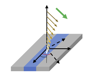
For fluid flows in contact with SH and CP surfaces having longitudinal or transverse groove (stripe) orientations (i.e. with respect to the flow direction), the pressure gradient and the slip velocity vectors are unidirectional (Belyaev & Vinogradova Reference Belyaev and Vinogradova2010; Vinogradova & Belyaev Reference Vinogradova and Belyaev2011). However, a secondary flow stream is generated normal to the pressure gradient direction in an oblique groove configuration, in which the direction of the grooves makes an angle  $0< \theta < 90^\circ$ with respect to the direction of the applied pressure gradient (see figure 1); this is due to the directional anisotropic slip properties of the surface (Stone, Stroock & Ajdari Reference Stone, Stroock and Ajdari2004; Bazant & Vinogradova Reference Bazant and Vinogradova2008; Vinogradova & Belyaev Reference Vinogradova and Belyaev2011). Therefore, such an oblique configuration leads to unique flow features that can be exploited for many applications, e.g. passive mixing and flow/particle manipulation (Stroock et al. Reference Stroock, Dertinger, Whitesides and Ajdari2002a,Reference Stroock, Dertinger, Ajdari, Mezic, Stone and Whitesidesb; Asmolov et al. Reference Asmolov, Dubov, Nizkaya, Harting and Vinogradova2018; Vagner & Patlazhan Reference Vagner and Patlazhan2019; Nizkaya et al. Reference Nizkaya, Asmolov, Harting and Vinogradova2020).

Figure 1. Schematic of oblique Poiseuille flow of a Bingham fluid in an SH channel (for the CP channel the groove would be replaced by a flat slippery stripe). Pressure gradient is in  $\hat z'$ direction at an angle $\theta$ with $\hat z$ axis. Right panel shows $s$ as the a priori unknown angle between slip velocity vector and groove direction. Here and throughout the text, the dimensional parameters and variables are shown with the hat sign $\widehat {(\cdot)}$ whereas for the dimensionless parameters and variables the hat sign is dropped (unless otherwise stated).
Our article presents a novel contribution to the analysis of viscoplastic flows in channels with longitudinal, transverse and most importantly oblique groove (stripe) orientations. Unlike the oblique flow of a Newtonian fluid, whose model equations can be solved via a linear vector transformation of known longitudinal and transverse flow variables (Bazant & Vinogradova Reference Bazant and Vinogradova2008; Vinogradova & Belyaev Reference Vinogradova and Belyaev2011), the oblique flow of a viscoplastic fluid requires a distinct solution due to its nonlinear viscosity, implying that the transform matrix is unknown a priori. To address this challenge, here we consider the creeping Poiseuille flow of a Bingham fluid in thick patterned channels (where the half-channel height  $\hat H$ is much larger than the pattern (i.e. groove or stripe) period $\hat L$, as illustrated in figure 1). In addition, we consider flow slippage on the patterned wall, assuming a flat liquid/air interface pinned at the groove edges for the SH wall and a flat slippery stripe for the CP wall, while employing the Navier slip law and the no-slip condition to account for the patterned wall condition. Using perturbation analysis, Fourier expansion method and dual trigonometric series solution (Sneddon Reference Sneddon1966), we develop a comprehensive model for viscoplastic flows in SH and CP channels; this includes semi-analytical, explicit-form and computational fluid dynamics (CFD) models, which allow us to systematically analyse the flow parameters effects on the key characteristics of our complex flow dynamics.
The present article is structured as follows. In § 2, we introduce the flow governing equations, followed by § 3 where we develop our mathematical models for calculating the perturbation and slip velocities. In § 4, we discuss additional flow features, such as the total velocity profile, effective slip length tensor, slip angle and flow mixing index. The numerical simulation setup is described in § 5. In § 6, we present the results and, in § 7, we provide a summary of the main findings of our work.
2. Governing equations
2.1. Equations of motion
This section presents our plane Poiseuille flow of a Bingham fluid with an SH (or CP) lower wall, including the governing continuity and momentum balance equations, in a Cartesian coordinate system  $(x,y,z)$ (see figure 1). Motivated by practical considerations, we consider a channel where the lower boundary is a groovy wall and the upper boundary has a no-slip condition; this is because, in practice, the construction of a channel with two symmetrically aligned patterned walls, typically on the micro- or nano-scale, is challenging (Schmieschek et al. Reference Schmieschek, Belyaev, Harting and Vinogradova2012) (we later discuss the extension of our models for the channels with two patterned walls in Appendix F). Considering a creeping flow motion, the dimensionless forms of the continuity and momentum balance equations are
 $$\begin{gather} \boldsymbol{\nabla}\boldsymbol{\cdot}{\boldsymbol{U}} = 0, \end{gather}$$
 $$\begin{gather}- \boldsymbol{\nabla} P + \boldsymbol{\nabla}\boldsymbol{\cdot}{\boldsymbol{\tau }} = 0, \end{gather}$$
where  $t$ is the time, ${\boldsymbol {U} = U{\boldsymbol {e}_x} + V{\boldsymbol {e}_y} + W{\boldsymbol {e}_z}}$ is the dimensionless velocity vector, $P$ is the pressure and the deviatoric stress tensor is denoted by ${\boldsymbol {\tau }}$. The pressure gradient is in the $z'$ direction, which is at an angle $\theta$ with the $z$ axis (see figure 1). The dimensionless form of the equations of motion is obtained by considering the half-channel height ( $\hat H$) as the characteristic length and the average velocity ( $\hat U_{ave}$) as the velocity scale. In addition, the characteristic viscous stress, i.e. $\hat \mu _p ({\hat U_{ave}}/{\hat H})$ where $\hat \mu _p$ is the plastic viscosity, is used to obtain the dimensionless form of the pressure and stress terms.
The Bingham constitutive equation is considered to model the viscoplastic rheology, which in dimensionless form is presented as
 \begin{equation} \left\{\begin{array}{@{}ll} {\boldsymbol {\tau }} = \left( {1 + \dfrac{B}{{\dot \gamma }}} \right) {\boldsymbol {\dot \gamma }}, & \tau > B,\\ \boldsymbol{\dot \gamma} = 0, & \tau \le B, \end{array}\right. \end{equation}
where the strain rate tensor is shown by  ${\boldsymbol {\dot \gamma } = \boldsymbol {\nabla } \boldsymbol {u} + {( {\boldsymbol {\nabla } \boldsymbol {u}} )^{\rm T}}}$, and the norms (magnitudes) of the stress and strain rate tensors are ${\tau = \sqrt {{{{\tau _{ij}}{\tau _{ij}}}/2}}}$ and ${\dot \gamma = \sqrt {{{{{\dot \gamma }_{ij}}{{\dot \gamma }_{ij}}}/2}}}$, respectively (here, $i$ and $j$ refer to the coordinate axes, i.e. $x$,
$x$,  $y$ and $z$). The ratio of the yield stress ( ${{{\hat \tau _0}}}$) to the characteristic viscous stress is represented by the Bingham number and defined as
 \begin{equation} B = \frac{{{\hat \tau _0}\hat H}}{{{{\hat \mu }_p}{{\hat U}_{ave}}}}. \end{equation}
Based on (2.3), formation of plug zones are expected for a viscoplastic flow when the applied stress is smaller than the yield stress. For example, formation of an unyielded plug zone in the channel centre is a characteristic of the creeping Poiseuille flow of viscoplastic materials. Based on (2.3), at the yield surfaces and inside the plug, the strain-rate tensor and its norm vanish.
2.2. No-slip base flow
Given the symmetry condition for the no-slip base flow, i.e. with the no-slip condition at both walls, the base flow pressure ( $P_0^b$) and velocity ( $U^b_0$) for the lower half of the channel can be easily derived as
 $$\begin{gather} P_0^b ={-} {\tau _w}z' + {\text{constant}}, \end{gather}$$
 $$\begin{gather}{U^b_0}(\kern0.7pt y) = \left\{\begin{array}{@{}ll} {C_1}y + {C_2}{y^2}, & 0 \le y \le {h_0}, \\ {C_3}, & {h_0} \le y \le 1, \end{array}\right. \end{gather}$$
where  $C_1=\tau _w - B$, $C_2=-({\tau _w}/{2})$, $C_3={(\tau _w - B)^2}/{2\tau _w}$ and $h_0$ denotes the location of the lower yield surface. The wall shear stress, $\tau _w$, at $y=0$ corresponds to the largest positive root of the following equation:
 \begin{equation} 2\tau _w^3 - (3B + 6)\tau _w^2 + {B^3} = 0. \end{equation}
Subsequently, one can find the location of lower yield surface as
 \begin{equation} {{h_0} = 1 - \frac{B}{{{\tau _w}}}}. \end{equation}
Since the  $U^b_0$ vector is in the $z'$ direction, the base no-slip velocity has two components in the $x$ and $z$ directions, i.e. $U_0=U^b_0 \sin \theta$ and $W_0=U^b_0 \cos \theta$, respectively.
2.3. Slip model
The linear Navier slip law is considered to account for the Bingham fluid slippage on the interface. Therefore, the following relation for the slip velocities in the  $z$ (
$z$ ( $w_s$) and $x$ (
$x$ ( $u_s$) directions is derived for the Bingham fluid:
 \begin{equation} \{ {{w_s},{u_s}}\} = b{\{ {{\tau _{yz}},{\tau _{xy}}}\}_{y = 0}}, \end{equation}
where  $b$ represents the dimensionless slip number, defined as $b = {{\hat b {\hat \mu }_p}/{\hat H}}$. Here, $\hat b$ is the dimensional slip number, correlating the dimensional values of the slip velocity and shear stress.
Based on the analyses developed for the Newtonian flows (Schönecker & Hardt Reference Schönecker and Hardt2013; Nizkaya, Asmolov & Vinogradova Reference Nizkaya, Asmolov and Vinogradova2014; Schönecker, Baier & Hardt Reference Schönecker, Baier and Hardt2014), in general,  $\hat b$ can be related to the air viscosity ( $\hat \mu _a$) and the groove aspect ratio ( $A_r=\hat d/\hat \delta$). In addition, $\hat b$ (and, hence, $b$) has been proven to show a tensorial form for SH surfaces, i.e. with different values of the local slip length (number) in the longitudinal and transverse directions. For large values of the local slip length, where the flow condition on the liquid/air interface approaches the no-shear condition, the tensorial form of $\hat b$ (and, hence, $b$) becomes less important and can be effectively replaced by a scalar form, i.e. an equal value can be considered for the slip number in both the longitudinal and transverse directions (Schönecker & Hardt Reference Schönecker and Hardt2013; Nizkaya et al. Reference Nizkaya, Asmolov and Vinogradova2014; Schönecker et al. Reference Schönecker, Baier and Hardt2014). On the other hand, for the CP surfaces, the local slip length can be identical in the longitudinal and transverse conditions, rendering a scalar form of the slip number (Qian et al. Reference Qian, Wang and Sheng2005; Wang et al. Reference Wang, Qian and Sheng2008; Lee et al. Reference Lee, Charrault and Neto2014). Since the tensorial form of the slip number has not yet been explored for the viscoplastic flows (refer to the discussion in § 7), here we assume a scalar form of the slip number, i.e. a similar value of $\hat b$ (and, hence, $b$) for longitudinal, transverse and oblique configurations. However, assuming a tensorial slip number, i.e. any functionality of $\hat b$ (and, hence, $b$) with respect to the angle $\theta$, the models developed in this study would remain valid (see preliminary tensorial form analysis of the local slip number in Appendix D). We may expect that the assumed scalar form for the slip number can provide us with reasonably accurate predictions of the flow dynamics over the CP surfaces, while capturing leading physical trends for the flow over SH surfaces at large values of the slip number. In addition, the upcoming solutions may provide some insight about the viscoplastic flow dynamics over the liquid-infused (LI) surfaces; however, to provide accurate results for this case, the exact tensorial form of the slip number must be employed and the corresponding scalar form is not valid (Schönecker et al. Reference Schönecker, Baier and Hardt2014).
Before proceeding, it is worth mentioning that both the groove (stripe) period (width) (Sbragaglia & Prosperetti Reference Sbragaglia and Prosperetti2007; Hodes et al. Reference Hodes, Kirk, Karamanis and MacLachlan2017; Game, Hodes & Papageorgiou Reference Game, Hodes and Papageorgiou2019) and channel height (or pipe diameter) (Lauga & Stone Reference Lauga and Stone2003; Schnitzer & Yariv Reference Schnitzer and Yariv2017, Reference Schnitzer and Yariv2019; Kirk et al. Reference Kirk, Karamanis, Crowdy and Hodes2020) have been used within the literature as the characteristic lengths to make the slip length dimensionless. In this work, for definition of the slip number, i.e.  $b={\hat b \hat \mu _p}/{\hat H}$, the half-channel height ( $\hat H$) is used as the characteristic length. Although employing the groove (stripe) period ( $\hat L$) as the characteristic length can be useful when interpreting the local slip dynamics on the patterned wall, our definition of the slip number is also physically relevant, as it provides an understanding regarding the overall patterned wall effects on the channel flow dynamics. In addition, the defined dimensionless slip number in our work can be simply converted to the slip number that is made dimensionless using the groove (stripe) period ( $b_L$) as $b_L=b/\ell$. Therefore, one can also use such a conversion to be able to interpret the results, if required. In addition, the usage of $\hat H$ as the characteristic length is prevalent and advantageous in defining the Bingham number ( $B$), which is a key parameter of our viscoplastic flow.
3. Mathematical modelling
3.1. Perturbation equations
In this work, semi-analytical and explicit-form solutions are developed for the Poiseuille flow of Bingham fluids in channels with a patterned wall, considering the limiting cases of longitudinal ( $\theta =0$) and transverse ( $\theta =90^\circ$) grooves (stripes), as well as the general case of the oblique ( $0 < \theta < 90^\circ$) flow configuration. These solutions are developed for the thick channel limit ( $\ell ={\hat {L}}/{\hat {H}} \ll 1$), where the lower yield surface (located at $y=h$) remains flat (Rahmani & Taghavi Reference Rahmani and Taghavi2022). The solution can be derived by considering infinitesimal perturbations induced by the patterned wall (with respect to the no-slip flow) in the lower yielded zone ( $-\ell /2 \le x \le \ell /2$ and $0 \le y < h$) and solving for the leading-order terms. Therefore, the total velocity vector ( $\boldsymbol {U}$) is written as
 \begin{equation} \boldsymbol{U}=\boldsymbol{U}_0+\epsilon \boldsymbol{u}, \end{equation}
where  $\boldsymbol {U}_0 = U_0{\boldsymbol {e}_x} + W_0{\boldsymbol {e}_z}$, i.e. $(U_0,0,W_0)$, represents the no-slip velocity vector and
 \begin{equation} \boldsymbol{u} = u{\boldsymbol {e}_x} + v{\boldsymbol {e}_y} + w{\boldsymbol {e}_z} \end{equation}
shows the perturbation velocity vector  $(u,v,w)$. Here, $\epsilon =\kappa ^{-1}$ is the perturbation parameter where $\kappa =2{\rm \pi} /\ell$ is the patterned wall wavenumber. Based on this perturbation method, the effective viscosity of the Bingham fluid ( $\mu$) and the stress components are expanded as follows:
 $$\begin{gather} \mu (\boldsymbol{U_0} + \epsilon \boldsymbol{u}) = \mu (\boldsymbol{U_0}) + \epsilon {\dot \xi _{ij}}(\boldsymbol{u})\frac{{\partial \mu }}{{\partial {{\dot \gamma }_{ij}}}} (\boldsymbol{U_0}) + O({\epsilon ^2}), \end{gather}$$
 $$\begin{gather}{\tau _{ij}} (\boldsymbol{U_0} + \epsilon \boldsymbol{u}) = {\tau _{ij}}(\boldsymbol{U_0}) + \epsilon {\sigma _{ij}}(\boldsymbol{u}) + O({\epsilon ^2}), \end{gather}$$
where  $\dot \xi _{ij}$ and $\sigma _{ij}$ represent the component of the perturbation strain-rate and stress tensor, respectively. Henceforth, for presentation simplicity, we use $\mu _0=\mu (\boldsymbol {U_0})$.
3.1.1. Longitudinal configuration
For the longitudinal groove (stripe) configuration, the no-slip and perturbation velocity vectors reduce to ( $0,0,W_0$) and ( $0,0,w$), respectively. In addition, considering an infinitely long channel in both x and z directions, the velocity gradients in the $z$ direction are zero ( $\partial \boldsymbol{U} /\partial z = 0$, a feature valid for any angle of $\theta$), only two non-zero perturbation stress components remain for the Bingham fluid as
 \begin{equation} \left.\begin{gathered} {\sigma _{yz}} = \frac{{\partial w}}{{\partial y}}, \\ {\sigma _{xz}} = \mu_0 \frac{{\partial w}}{{\partial x}}, \end{gathered}\right\} \end{equation}
where  $\mu _0=1+{B}/{({\rm d} U^b_0/{{\rm d}y})}$. Therefore, the perturbed momentum balance equation shrinks to
 \begin{equation} \mu_0 \frac{{{\partial ^2}w}}{{\partial {x^2}}} + \frac{{{\partial ^2}w}}{{\partial {y^2}}} = 0, \end{equation}
in which the perturbation parameter is dropped.
In the present study, to facilitate the identification of various orders of perturbed momentum balance equations for a given flow configuration, a rescaling is introduced as
 \begin{equation} \epsilon X=x,\quad \epsilon Y=y,\quad \epsilon \varPsi=\psi, \end{equation}
where  $\psi$ is the perturbation stream function such that $u = {{\partial \psi }}/{{\partial y}}$ and $v = -{{\partial \psi }}/{{\partial x}}$. The introduced rescaling is motivated by the decay of perturbations in the $y$ direction, which renders the perturbation negligible beyond a distance comparable to the groove periodicity length. Consequently, the rescaled distance over which the perturbation field is considerable becomes of order $\epsilon ^0$. Thus, we may expand the viscosity over $Y=0$ to reach
 \begin{equation} \mu_0=1+\frac{B}{C_1}-\epsilon \left(\frac{2BC_2}{C_1^2}\right) Y, \end{equation}
in which coefficients  $C_1$ and $C_2$ are given in § 2.2. Therefore, the rescaled form of (3.6) for the leading-order terms is obtained as
 \begin{equation} \left(1+\frac{B}{C_1}\right) \frac{{{\partial ^2}w}}{{\partial {X^2}}} + \frac{{{\partial ^2}w}}{{\partial {Y^2}}} = 0, \end{equation}
where  $\epsilon$ drops from (3.9).
Following the convention in the field (Lauga & Stone Reference Lauga and Stone2003; Belyaev & Vinogradova Reference Belyaev and Vinogradova2010; Vinogradova & Belyaev Reference Vinogradova and Belyaev2011), we consider our creeping flow to be periodic in the  $x$ direction with a period of $\ell$. Accordingly, in the rescaled system, the flow is periodic in the $X$ direction with a period of $2{\rm \pi}$. Therefore, the solution for $w$ can be written in the Fourier series form as
 \begin{equation} w (X,Y) = \sum_{n = 0 }^\infty {B_n}{\hat w_n } (Y){\cos ({nX})}, \end{equation}
where  $B_n$ are unknown coefficients that will be calculated later with the use of appropriate patterned wall conditions. Here, the hat sign is used to define the Fourier coefficient (i.e. $\hat w_n$).
Substituting (3.10) into (3.9), one can find the following ordinary differential equation (ODE):
 \begin{equation} \frac{{{{\rm d}^2}\hat w_n}}{{{\rm d} {Y^2}}} - \left(1+\frac{B}{C_1}\right){n^2}\hat w_n = 0. \end{equation}
To close the boundary value problem, the following boundary conditions are considered ( $n \ne 0$):
 \begin{equation} \hat w_n(\kappa h) = 0,\quad \frac{{{\rm d} \hat w_n}}{{{\rm d} Y}}(\kappa h) = 0, \end{equation}
where the first and second conditions from left to right ensure zero perturbation velocity and zero strain-rate magnitude at the lower yield surface ( $Y=\kappa h$), respectively. The zeroth term ( $n=0$) has a linear distribution in $Y$ and is discussed later in § 3.2.
3.1.2. Transverse configuration
In the transverse configuration, the no-slip and perturbation velocity vectors reduce to  $(U_0,0,0)$ and $(u,v,0)$, respectively. Perturbing the momentum balance equation, eliminating the pressure, using the definition of $\varPsi$, considering the rescaling, and expanding $\mu _0$, the following partial differential equation is eventually derived at the leading order:
 \begin{equation} \frac{{{\partial ^4}\varPsi }}{{\partial {X^4}}} + \frac{{{\partial ^4}\varPsi }}{{\partial {Y^4}}} + \left( {2 + \frac{{4B}}{{{C_1}}}} \right)\frac{{{\partial ^4}\varPsi }}{{\partial {X^2}\partial {Y^2}}} = 0, \end{equation}
where  $\epsilon$ drops from (3.13). Considering the flow periodicity in $X$, one can write
 \begin{equation} \varPsi (X,Y) = \sum_{n = 0 }^\infty {A_n}{\hat \varPsi_n } (Y){\cos ({nX})}, \end{equation}
where  $A_n$ are unknown coefficients and will be obtained later using the patterned wall condition. Here, the hat sign is used to define the Fourier coefficient (i.e. $\hat \varPsi _n$).
Substituting (3.14) into (3.13), we find the following ODE:
 \begin{equation} \frac{{{{\rm d}^4}\hat \varPsi_n }}{{{\rm d} {Y^4}}} - \left( {2 + \frac{{4B}}{{{C_1}}}} \right){n^2} \frac{{{{\rm d}^2}\hat \varPsi_n }}{{{\rm d} {Y^2}}} + {n^4}\hat \varPsi_n = 0. \end{equation}
To close the boundary value problem, we consider the following conditions ( $n \ne 0$)
 \begin{equation} \hat \varPsi_n (0) = 0,\quad \hat \varPsi_n (\kappa h) = 0,\quad \frac{{{\rm d} \hat \varPsi_n }}{{{\rm d} Y}}(\kappa h) = 0,\quad \frac{{{{\rm d}^2}\hat \varPsi_n }}{{{\rm d} {Y^2}}}(\kappa h) = 0, \end{equation}
where the first condition from left to right ensures the no-penetration assumption at the patterned wall (i.e.  $V=0$ at $Y=0$). The zero perturbation velocity field at the lower yield surface ( $Y=\kappa h$) is guaranteed using the second and third conditions (from left to right). Finally, the zero strain-rate magnitude at the lower yield surface is obtained using the fourth condition. Here, the zeroth term ( $n=0$) would show a quadratic functionality of $Y$, as discussed in § 3.2.
3.1.3. Oblique configuration
In the oblique configuration, the no-slip and perturbation velocity vectors, i.e.  $(U_0,0,W_0)$ and $(u,v,w)$, respectively, have their most general forms. Accordingly, the perturbation stress components can be obtained as given in Appendix A. Then, using the definition of $\varPsi$, adopting the rescaling introduced in (3.7a–c), expanding $\mu _0$ via (3.8) and performing considerable algebra, we derive a set of two coupled partial differential equations for $\varPsi$ and $w$ at the leading order:
 \begin{gather} {\left(1+\frac{B}{C_1}\right)}\left( {\frac{{{\partial
^4}\varPsi }}{{\partial {X^4}}} + \frac{{{\partial
^4}\varPsi }}{{\partial {Y^4}}} + 2\frac{{{\partial
^4}\varPsi }}{{\partial {X^2}\partial {Y^2}}}} \right) -
{\frac{B}{C_1}}\left( {\frac{{{\partial ^4}\varPsi
}}{{\partial {X^4}}} + \frac{{{\partial ^4}\varPsi
}}{{\partial {Y^4}}} - 2\frac{{{\partial ^4}\varPsi
}}{{\partial {X^2}\partial {Y^2}}}} \right){\sin ^2}\theta
\nonumber\\ -{\frac{B}{C_1}}\left( {\frac{{{\partial
^3}w}}{{\partial {Y^3}}} - \frac{{{\partial
^3}w}}{{\partial {X^2}\partial Y}}} \right) \sin \theta
\cos \theta = 0, \end{gather}
\begin{gather} {\left(1+\frac{B}{C_1}\right)}\left( {\frac{{{\partial
^4}\varPsi }}{{\partial {X^4}}} + \frac{{{\partial
^4}\varPsi }}{{\partial {Y^4}}} + 2\frac{{{\partial
^4}\varPsi }}{{\partial {X^2}\partial {Y^2}}}} \right) -
{\frac{B}{C_1}}\left( {\frac{{{\partial ^4}\varPsi
}}{{\partial {X^4}}} + \frac{{{\partial ^4}\varPsi
}}{{\partial {Y^4}}} - 2\frac{{{\partial ^4}\varPsi
}}{{\partial {X^2}\partial {Y^2}}}} \right){\sin ^2}\theta
\nonumber\\ -{\frac{B}{C_1}}\left( {\frac{{{\partial
^3}w}}{{\partial {Y^3}}} - \frac{{{\partial
^3}w}}{{\partial {X^2}\partial Y}}} \right) \sin \theta
\cos \theta = 0, \end{gather}
 \begin{gather} {\left(1+\frac{B}{C_1}\right)}\left( {\frac{{{\partial ^2}w}}{{\partial {X^2}}} + \frac{{{\partial^2}w}}{{\partial {Y^2}}}} \right) -{\frac{B}{C_1}} \frac{{{\partial ^2}w}}{{\partial {Y^2}}}{\cos^2}\theta -{\frac{B}{C_1}}\left( {\frac{{{\partial ^3}\varPsi }}{{\partial {Y^3}}} - \frac{{{\partial ^3}\varPsi }}{{\partial {X^2}\partial Y}}}\right) \sin \theta \cos \theta = 0, \end{gather}
where  $\epsilon$ is dropped from the above equations. Equations (3.17) and (3.18) are unique to viscoplastic Bingham materials, significantly differing from the corresponding equations for Newtonian fluids. In the case of Newtonian fluids, we have $B=0$ (i.e. $\mu _0=1$; see (3.8)); consequently, (3.17) and (3.18) decouple, and become independent of $\theta$, i.e. reducing to the corresponding equations for the transverse and longitudinal flows, respectively. Thus, for Newtonian fluids, it suffices to solve the perturbed equation only for the longitudinal and transverse configurations, and the solution for the oblique configuration can be simply obtained via a linear vector transformation through the transform (or rotation) matrix (Bazant & Vinogradova Reference Bazant and Vinogradova2008; Vinogradova & Belyaev Reference Vinogradova and Belyaev2011). Therefore, it is clear that the nonlinear viscoplastic rheology sets our work apart from the Newtonian case, and it plays a crucial role in determining the slip dynamics on a patterned wall, i.e. a feature that we address in this study.
Considering the flow periodicity in the  $X$ direction, one can substitute (3.10) and (3.14) into (3.17) and (3.18) to arrive at the following coupled ODEs:
 \begin{align} & {A_n}\left[ {{\left(1+\frac{B}{C_1}\right)}\left({\frac{{{{\rm d}^4}\hat \varPsi_n }}{{{\rm d} {Y^4}}} - 2{n^2} \frac{{{{\rm d}^2}\hat \varPsi_n }}{{{\rm d} {Y^2}}} + {n^4}\hat \varPsi_n}\right) -{\frac{B}{C_1}}\left({\frac{{{{\rm d}^4}\hat \varPsi_n }}{{{\rm d} {Y^4}}} + 2{n^2} \frac{{{{\rm d}^2}\hat \varPsi_n }}{{{\rm d} {Y^2}}} + {n^4}\hat \varPsi_n } \right){{\sin }^2}\theta } \right] \nonumber\\ &\quad -{B_n}{\frac{B}{C_1}}\left( {\frac{{{{\rm d}^3}\hat w_n}}{{{\rm d} {Y^3}}} + {n^2}\frac{{{\rm d} \hat w_n}}{{{\rm d} Y}}} \right)\sin \theta \cos \theta = 0, \end{align}
 \begin{align} & -{A_n}{\frac{B}{C_1}}\left( {\frac{{{{\rm d}^3}\hat \varPsi_n }}{{{\rm d} {Y^3}}} + {n^2}\frac{{{\rm d} \hat \varPsi_n }}{{{\rm d} Y}}} \right)\sin \theta \cos \theta \nonumber\\ &\quad + {B_n}{\left[ {{\left(1+\frac{B}{C_1}\right)}\left( {\frac{{{{\rm d}^2}\hat w_n}}{{{\rm d} {Y^2}}} - {n^2}\hat w_n} \right) -{\frac{B}{C_1}}\frac{{{{\rm d}^2}\hat w_n}}{{{\rm d} {Y^2}}}{{\cos }^2}\theta } \right] = 0.} \end{align}
The boundary conditions for these equations are the combination of those for the longitudinal and transverse configurations, i.e. (3.12a,b) and (3.16a–d). In addition, the zeroth term solutions ( $n=0$) are treated similar to those of the longitudinal and transverse configurations and are discussed further in § 3.2.
3.2. Semi-analytical solution
In this section, we attempt to solve the ODEs (3.11), (3.15), (3.19) and (3.20). These ODEs have constant coefficients; thus, the solutions for  $\hat \varPsi _n$ and $\hat w_n$ would be in the form ${\rm e}^{\varLambda _n Y}$. In the thick channel limit, since the perturbation field quickly decays in the $Y$ direction, the contribution of the terms having positive ${\varLambda _n}$, i.e. $\varLambda _n>0$, becomes negligible. In other words, one can simply show that the terms with positive ${\varLambda _n}$ belong to the higher orders of perturbations. Therefore, in the following sections, the solutions for $\hat \varPsi _n$ and $\hat w_n$ are obtained considering only the terms with negative ${\varLambda _n}$.
Before proceeding, let us consider the perturbation velocity field as  $\boldsymbol u$ instead of $\epsilon \boldsymbol u$ in the following sections. This consideration leads to having simpler forms of equations, as the redundant $\epsilon$ symbol disappears.
3.2.1. Longitudinal configuration
For the longitudinal configuration, (3.11) is solved analytically, keeping the term with the negative  ${\varLambda _n}$, as
 \begin{equation} {\hat w_n}(Y) = {\exp({ - {\lambda ^\parallel } nY})},\quad {\lambda ^\parallel } = \sqrt {1 + \frac{B}{C_1}}, \end{equation}
where the symbol  $\parallel$ represents the longitudinal flow, henceforth. The expression obtained for $\hat w_n$ would satisfy the conditions of (3.12a,b), since at $Y=\kappa h$, i.e. the lower yield surface, $\hat w_n$ and ${\rm d}\hat w_n/{\rm d} Y$ become negligible and belong to the higher orders of perturbation. After solving for $\hat w_n$, the solution for $w$ can be written in the following form:
 \begin{equation} w(X,Y) = {B_0}\left( {1 - \frac{Y}{\kappa h}} \right) + \sum_{n = 1}^\infty {{B_n}} \hat w_n (Y)\cos (nX), \end{equation}
where the zeroth term solution has a linear distribution in  $Y$ and satisfies the zero perturbation velocity condition at the lower yield surface, i.e. $Y=\kappa h$. The remaining condition to be satisfied by the zeroth term solution is the zero strain-rate magnitude at the lower yield surface, which is satisfied through numerical iterations on $h$, as explained in § 4.1.1.
For the longitudinal configuration, the boundary conditions at the patterned wall is obtained as
 $$\begin{gather} {w}(X,0) - b{\left( {B + C_1 + \kappa \frac{{\partial w}}{{\partial Y}}} \right)_{Y = 0}} = 0,\quad 0 \leq X \leq {\rm \pi}\varphi, \end{gather}$$
 $$\begin{gather}{w}(X,0) = 0,\quad {\rm \pi}\varphi \leq X \leq {\rm \pi}, \end{gather}$$
where  $\varphi ={\hat \delta }/{\hat L}$ is called the slip area fraction and represents the fraction of the patterned wall that undergoes the slip condition. Equations (3.23) and (3.24) together represent the patterned wall condition that has been already discussed.
After substituting the solution for the perturbation velocity field, i.e. (3.22), into the patterned wall condition, i.e. (3.23) and (3.24), the following dual trigonometric series problem emerges:
 $$\begin{gather} {B_0}\left( {1 + \frac{b}{h}} \right) + \sum_{n = 1}^\infty {{B_n}} \left[ {{{\hat w}_n}(0) - b\kappa{\frac{{\rm d}\hat w_n}{{\rm d} Y}(0)}} \right]\cos ({nX}) = b({B + {C_1}}),\quad 0 \leq X \leq {\rm \pi}\varphi, \end{gather}$$
 $$\begin{gather}{B_0} + \sum_{n = 1}^\infty {{B_n}} {{\hat w}_n}(0)\cos ({nX}) = 0,\quad {\rm \pi}\varphi \leq X \leq {\rm \pi}. \end{gather}$$
 To calculate the unknown coefficients  $B_n$ ( $n=0,1,2,\ldots$), we first integrate (3.25) in $[0\ X]$ and then multiply it by ${\sin }(mX)$, where $m$ is a positive integer. Afterwards, we integrate the resulting equation in $[0\ {\rm \pi}\varphi ]$. Second, we multiply (3.26) by ${\cos }(mX)$ and then integrate it in $[{\rm \pi} \varphi \ {\rm \pi}]$. After the summation of the obtained terms, we establish a system of linear equations (truncated at the $N$th term):
 \begin{equation} \sum_{n = 0}^N {{P_{mn}^{{\parallel}}}{B_n}} = {M_m^{{\parallel}}}, \end{equation}
where the above coefficient and constant matrices are obtained as
 $$\begin{gather} {P_{m0}^{{\parallel}}} = \left( {1 + \frac{b}{h}} \right) I_3+ I_4, \end{gather}$$
 $$\begin{gather}{P_{mn}^{{\parallel}}} = \frac{1}{{n}}\left[ {{{\hat w}_n}(0) - b\kappa{\frac{{\rm d}\hat w_n}{{\rm d} Y}(0)}} \right] I_1 + {{\hat w}_n}(0) I_2,\quad n>0, \end{gather}$$
 $$\begin{gather}{M_m^{{\parallel}}} = b\left( {B + {C_1}} \right) I_3, \end{gather}$$
where  $I_1$, $I_2$, $I_3$ and $I_4$ are the following integrals
 $$\begin{gather} I_1 = \int_0^{{\rm \pi} \varphi } {\sin } (nX)\sin (mX)\,{\rm d} X, \end{gather}$$
 $$\begin{gather}I_2 = \int_{{\rm \pi} \varphi }^{\rm \pi} {\cos } (nX)\cos (mX)\,{\rm d} X, \end{gather}$$
 $$\begin{gather}I_3 = \int_0^{{\rm \pi} \varphi } X \sin (mX)\,{\rm d} X, \end{gather}$$
 $$\begin{gather}I_4 = \int_{{\rm \pi} \varphi }^{\rm \pi} \cos (mX)\,{\rm d} X. \end{gather}$$
3.2.2. Transverse configuration
Solving the ODE (3.15) while keeping the terms with negative  ${\varLambda _n}$, we find
 \begin{align} {\hat \varPsi _n}\left( Y \right) = {{\exp({ - \lambda _1^ \bot nY})} - {\exp({ - \lambda _2^ \bot nY})}},\quad \left\{\begin{array}{@{}l} \lambda _1^ \bot = \dfrac{{\sqrt {{C_1}({2B + {C_1} + 2\sqrt {{B^2} + B{C_1}}})} }}{{{C_1}}},\\ \lambda _2^ \bot = \dfrac{{\sqrt {{C_1}({2B + {C_1} - 2\sqrt {{B^2} + B{C_1}}})} }}{{{C_1}}}, \end{array}\right. \end{align}
where the symbol  $\bot$ represents the transverse flow henceforth. The solution form developed previously for $\hat \varPsi _n$ satisfies the no-penetration condition at the patterned wall, i.e. $\hat \varPsi _n(0)=0$, hence $v(X,0)=0$ (see (3.38) further below). At $Y=\kappa h$, the values of $\hat \varPsi _n$, ${\rm d}\hat \varPsi _n/{\rm d} Y$ and ${\rm d}^2\hat \varPsi _n/{\rm d} Y^2$ become negligible and they belong to higher orders of perturbations; thus, the conditions of zero perturbation velocity and zero strain-rate magnitude at the lower yield surface are satisfied (for $n>0$ in the leading order). The zeroth term solution (i.e. $n=0$) would have a quadratic form for $\varPsi$, leading to a linear distribution for $u$ (similar to $w$). Again, the no-penetration condition at $Y=0$ and the zero perturbation velocity at the lower yield surface ( $Y=\kappa h$) is satisfied by the zeroth term solution. However, the condition of zero strain rate magnitude at the yield surface should be satisfied through an iterative approach on $h$, as described in § 4.1.1.
Having  $\hat \varPsi _n$, one can now write the solution for $\varPsi$, $u$ and $v$ as
 $$\begin{gather} \varPsi (X,Y) = {A_0} \left( {Y - \frac{{{Y^2}}}{{2\kappa h}}} \right) + \sum_{n = 1}^\infty {{A_n}} \hat \varPsi_n (Y)\cos ({nX}), \end{gather}$$
 $$\begin{gather}u(X,Y) = {A_0} \left({1 - \frac{Y}{\kappa h}} \right) + \sum_{n = 1}^\infty {{A_n}} {\frac{{\rm d}\hat \varPsi_n}{{\rm d} Y}(Y)} \cos ({nX}), \end{gather}$$
 $$\begin{gather}v(X,Y) = \sum_{n = 1}^\infty {{A_n}} \hat \varPsi_n (Y) n \sin ({nX}). \end{gather}$$
The patterned wall condition for the transverse configuration holds
 $$\begin{gather} {u}(X,0) - b{\left({ B + C_1 + \kappa\frac{{\partial u}}{{\partial Y}}} \right)_{Y = 0}} = 0,\quad 0 \leq X \leq {\rm \pi}\varphi, \end{gather}$$
 $$\begin{gather}{u}(X,0) = 0,\quad {\rm \pi}\varphi \leq X \leq {\rm \pi}. \end{gather}$$
Substituting (3.37) into (3.39) and (3.40) leads to a dual trigonometric series problem:
 $$\begin{gather} {A_0}\left( {1 + \frac{b}{h}} \right) + \sum_{n = 1}^\infty {{A_n}} \left[ {{\frac{{\rm d}\hat \varPsi_n}{{\rm d} Y}(0)} - b\kappa{\frac{{\rm d}^2\hat \varPsi_n}{{\rm d} Y^2}(0)}} \right]\cos ({nX}) = b({B + {C_1}}),\quad 0 \leq X \leq {\rm \pi}\varphi, \end{gather}$$
 $$\begin{gather}{A_0} + \sum_{n = 1}^\infty {{A_n}} {\frac{{\rm d}\hat \varPsi_n}{{\rm d} Y}(0)}\cos ({nX}) = 0,\quad {\rm \pi}\varphi \leq X \leq {\rm \pi}, \end{gather}$$
where (3.41) and (3.41) can be solved for  $A_n$, using the same method described for the longitudinal flow configuration. Thus, the following system is obtained
 \begin{equation} \sum_{n = 0}^N {{P_{mn}^{\bot}}{A_n}} = {M_m^{\bot}}, \end{equation}
where the coefficient and constant matrices for (3.43) are calculated as
 $$\begin{gather} {P_{m0}^{\bot}} = {P_{m0}^{{\parallel}}}, \end{gather}$$
 $$\begin{gather}{P_{mn}^{\bot}} = \frac{1}{{n}}\left[ {{\frac{{\rm d}\hat \varPsi_n}{{\rm d} Y}(0)} - b\kappa{\frac{{\rm d}^2\hat \varPsi_n}{{\rm d} Y^2}(0)}} \right] I_1 + {\frac{{\rm d}\hat \varPsi_n}{{\rm d} Y}(0)} I_2,\quad n>0, \end{gather}$$
 $$\begin{gather}{M_m^{\bot}} = {M_m^{{\parallel}}}. \end{gather}$$
3.2.3. Oblique configuration
Considering the solution for  $\hat w_n$ and $\hat \varPsi _n$ to be in the form of ${\rm e}^{\varLambda _nY}$, the ODEs (3.19) and (3.20) lead to the following relation:
 \begin{equation} \left(\begin{array}{@{}l@{}} {\varOmega_{11}}\quad {\varOmega_{12}}\\ {\varOmega_{21}}\quad {\varOmega_{22}} \end{array} \right)\left(\begin{array}{@{}l@{}} {A_n}\\ {B_n} \end{array}\right) = 0, \end{equation}
where
 $$\begin{gather} \varOmega_{11} = {\left(1+\frac{B}{C_1}\right)} (\varLambda_n^2 - n^2)^2 - \frac{B}{C_1} (\varLambda_n^2 + n^2)^2 \sin^2 \theta, \end{gather}$$
 $$\begin{gather}\varOmega_{22} = {\left(1+\frac{B}{C_1}\right)} (\varLambda_n^2 - n^2) - \frac{B}{C_1} \varLambda_n^2 \cos^2 \theta, \end{gather}$$
 $$\begin{gather}\varOmega_{12} ={-}\frac{B}{C_1} (\varLambda_n^2 + n^2) \varLambda_n \sin \theta \cos \theta, \end{gather}$$
 $$\begin{gather}\varOmega_{21}=\varOmega_{12}. \end{gather}$$
 In order to have non-zero solution for  $A_n$ and $B_n$, the determinant of the coefficient matrix in (3.47) should be zero; thus, $\varOmega _{11}\varOmega _{22}-\varOmega _{12}\varOmega _{21}=0$. This condition leads to finding six solutions for ${\varLambda _n}$, with three being negative. Keeping the terms with negative ${\varLambda _n}$, the solution for $\hat w_n$ and $\hat \varPsi _n$ can be written as (for $n>0$)
 $$\begin{gather} {\hat w_n}(Y) = {\exp({ - {\lambda_1 ^\angle } nY})}+\varGamma_n^{(1)} {\exp({ - {\lambda_2 ^\angle } nY})}+\varGamma_n^{(2)} {{\rm exp}(-nY)}, \end{gather}$$
 $$\begin{gather}{\hat \varPsi _n}(Y) = \varDelta^{(1)}_n{{\exp({ - \lambda _1^ \angle nY})} - {\exp({ - \lambda _2^ \angle nY})}}+\varDelta^{(2)}_n {{\rm exp}(-nY)}, \end{gather}$$
where the symbol  $\angle$ represents the oblique flow, henceforth, and
 $$\begin{gather} {\lambda _1^\angle }{ =
\frac{{\sqrt {{C_1}\left( {2B \,{+}\, {C_1} \,{-}\,
\dfrac{3}{2}B{{\cos }^2}\theta + 2\sqrt {{B^2} + B{C_1} +
\dfrac{9}{{16}}{B^2}{{\cos }^4}\theta \,{-}\, B{{\cos
}^2}\theta \left( {\dfrac{3}{2}B \,{+}\, {C_1}} \right)} }
\,\right)} }}{{{C_1}}},}
\end{gather}$$
$$\begin{gather} {\lambda _1^\angle }{ =
\frac{{\sqrt {{C_1}\left( {2B \,{+}\, {C_1} \,{-}\,
\dfrac{3}{2}B{{\cos }^2}\theta + 2\sqrt {{B^2} + B{C_1} +
\dfrac{9}{{16}}{B^2}{{\cos }^4}\theta \,{-}\, B{{\cos
}^2}\theta \left( {\dfrac{3}{2}B \,{+}\, {C_1}} \right)} }
\,\right)} }}{{{C_1}}},}
\end{gather}$$ $$\begin{gather}{\lambda _2^\angle }{ =
\frac{{\sqrt {{C_1}\left( {2B \,{+}\, {C_1} \,{-}\,
\dfrac{3}{2}B{{\cos }^2}\theta - 2\sqrt {{B^2} + B{C_1} +
\dfrac{9}{{16}}{B^2}{{\cos }^4}\theta \,{-}\, B{{\cos
}^2}\theta \left({\dfrac{3}{2}B \,{+}\, {C_1}} \right)} }
\,\right)} }}{{{C_1}}}.}
\end{gather}$$
$$\begin{gather}{\lambda _2^\angle }{ =
\frac{{\sqrt {{C_1}\left( {2B \,{+}\, {C_1} \,{-}\,
\dfrac{3}{2}B{{\cos }^2}\theta - 2\sqrt {{B^2} + B{C_1} +
\dfrac{9}{{16}}{B^2}{{\cos }^4}\theta \,{-}\, B{{\cos
}^2}\theta \left({\dfrac{3}{2}B \,{+}\, {C_1}} \right)} }
\,\right)} }}{{{C_1}}}.}
\end{gather}$$ The solution for each  $\hat w_n$ and $\hat \varPsi _n$ contains three terms; thus, for each solution, two coefficients are required in order to determine the contribution of each term to that solution, i.e. $\varGamma _n^{(1)}$ and $\varGamma _n^{(2)}$ for $\hat w_n$ and $\varDelta _n^{(1)}$ and $\varDelta _n^{(2)}$ for $\hat \varPsi _n$. Since the no-penetration condition should be satisfied at $Y=0$, one finds $\varDelta _n^{(2)}=1-\varDelta _n^{(1)}$. It is worth mentioning that the forms of solution written in (3.52) and (3.53) are comparable with those of the longitudinal and transverse configurations (3.21a,b) and (3.35a,b), as one might expect that when $\theta \to 0$, $\varGamma _n^{(1)} \to 0$ and $\varGamma _n^{(2)} \to 0$; however, when $\theta \to 90^\circ$, $\varDelta _n^{(1)} \to 1$ and, hence, $\varDelta _n^{(2)} \to 0$. One should also note that when $\theta \to 0$, $\lambda _1^\angle \to \lambda ^\parallel$ and once $\theta \to 90^\circ$, $\lambda _1^\angle \to \lambda _1^\bot$ and $\lambda _2^\angle \to \lambda _2^\bot$.
Substituting the solution terms for  $\hat w_n$ and $\hat \varPsi _n$ with identical ${\varLambda _n}$, e.g. ${\exp ({- {\lambda _1 ^\angle } nY})}$ and $\varDelta ^{(1)}_n{\exp ({ - \lambda _1^ \angle nY})}$, into (3.20), one can obtain following relations:
 $$\begin{gather} {\varDelta^{(1)} _n} ={-} \left( {\frac{{{B_n}}}{{{A_n}}}} \right){\left( {\frac{{{\varOmega _{22}}}}{{{\varOmega _{12}}}}} \right)_{\varLambda_n ={-}\lambda _1^\angle n }}, \end{gather}$$
 $$\begin{gather}\varGamma _n^{(1)} = \left( {\frac{{{A_n}}}{{{B_n}}}} \right){\left( {\frac{{{\varOmega _{12}}}}{{{\varOmega _{22}}}}} \right)_{\varLambda_n ={-}\lambda _2^\angle n }}, \end{gather}$$
 $$\begin{gather}\varGamma _n^{(2)} = ({{\varDelta^{(1)} _n} - 1})\left( {\frac{{{A_n}}}{{{B_n}}}} \right) {\left({\frac{{{\varOmega _{12}}}}{{{\varOmega _{22}}}}} \right)_{\varLambda_n ={-} n}}. \end{gather}$$
The numerical procedure for calculating the above-mentioned coefficients is discussed at the end of this section (i.e. § 3.2.3).
The solutions provided in (3.52) and (3.53) are for  $n>0$. Indeed, the solution form for $n=0$ of the oblique flow is identical to those of the longitudinal and transverse flow (i.e. the zero mode of the perturbation velocity is a linear function of $Y$). In fact, when considering $n=0$ in (3.52) and (3.53), the exponential forms vanish and the solutions for $n=0$ become similar to those obtained for the longitudinal and transverse flows (see (3.22) for $w_0$ and (3.36) for $\varPsi _0$).
In the oblique configuration, the patterned wall conditions are as follows:
 $$\begin{gather} w(X,0) - b{\left[
\begin{array}{@{}l@{}} ({B + C_1})\cos \theta \\ + \left( {1 +
\dfrac{B}{{{C_1}}}{{\sin}^2}\theta } \right){\kappa
}\dfrac{{\partial w}}{{\partial Y}}\\ - \dfrac{B}{C_1} \sin
\theta \cos \theta {\kappa }\dfrac{{\partial u}}{{\partial
Y}} \end{array}\right]_{Y = 0}} = 0,\quad 0 \le X \le {\rm \pi}
\varphi, \end{gather}$$
$$\begin{gather} w(X,0) - b{\left[
\begin{array}{@{}l@{}} ({B + C_1})\cos \theta \\ + \left( {1 +
\dfrac{B}{{{C_1}}}{{\sin}^2}\theta } \right){\kappa
}\dfrac{{\partial w}}{{\partial Y}}\\ - \dfrac{B}{C_1} \sin
\theta \cos \theta {\kappa }\dfrac{{\partial u}}{{\partial
Y}} \end{array}\right]_{Y = 0}} = 0,\quad 0 \le X \le {\rm \pi}
\varphi, \end{gather}$$
 $$\begin{gather}{w}(X,0) = 0,\quad {\rm \pi}
\varphi \leq X \leq {\rm \pi}.
\end{gather}$$
$$\begin{gather}{w}(X,0) = 0,\quad {\rm \pi}
\varphi \leq X \leq {\rm \pi}.
\end{gather}$$
 $$\begin{gather}u(X,0) - b{\left[
\begin{array}{@{}l@{}} ({B + C_1})\sin \theta \\ + \left( {1 +
\dfrac{B}{{{C_1}}}{{\cos}^2}\theta } \right){\kappa }
\dfrac{{\partial u}}{{\partial Y}}\\ - \dfrac{B}{C_1}\sin
\theta \cos \theta {\kappa } \dfrac{{\partial w}}{{\partial
Y}} \end{array}\right]_{Y = 0}} = 0,\quad 0 \le X \le {\rm \pi}
\varphi, \end{gather}$$
$$\begin{gather}u(X,0) - b{\left[
\begin{array}{@{}l@{}} ({B + C_1})\sin \theta \\ + \left( {1 +
\dfrac{B}{{{C_1}}}{{\cos}^2}\theta } \right){\kappa }
\dfrac{{\partial u}}{{\partial Y}}\\ - \dfrac{B}{C_1}\sin
\theta \cos \theta {\kappa } \dfrac{{\partial w}}{{\partial
Y}} \end{array}\right]_{Y = 0}} = 0,\quad 0 \le X \le {\rm \pi}
\varphi, \end{gather}$$
 $$\begin{gather}{u}(X,0) = 0,\quad {\rm \pi}\varphi \leq X \leq {\rm \pi}. \end{gather}$$
These coupled patterned wall conditions for the oblique configuration highlight the strong effects of the nonlinear viscoplastic rheology, since new terms emerge in the shear stress components originated from the nonlinear viscosity.
Substituting the solutions in the form of (3.22) and (3.37) into the patterned wall conditions, i.e. (3.59), (3.60), (3.61) and (3.62), the following dual trigonometric series problems emerge:
 \begin{align} & {B_0}\left( {1 + \frac{{b( {{C_1} + B{{\sin }^2}\theta})}}{{{C_1}h}}} \right) - {A_0}\left( {\frac{{bB\sin \theta \cos \theta }}{{{C_1}h}}} \right) \nonumber\\ &\qquad + \sum_{n = 1}^\infty {{B_n}} \left[ {{{\hat w}_n}(0) - b\left( {1 + \frac{B}{{{C_1}}}{{\sin }^2}\theta } \right)\kappa \frac{{{\rm d}{{\hat w}_n}}}{{{\rm d} Y}}(0)} \right]\cos ({nX}) \nonumber\\ &\qquad + \sum_{n = 1}^\infty {{A_n}} b\frac{B}{{{C_1}}}\sin \theta \cos \theta \kappa \frac{{{{\rm d}^2}{{\hat \varPsi }_n}}}{{{\rm d}{Y^2}}}(0)\cos ({nX}) \nonumber\\ &\quad = b({B + {C_1}})\cos \theta,\quad 0 \leq X \leq {\rm \pi}\varphi, \end{align}
 \begin{equation} {B_0} + \sum_{n = 1}^\infty {{B_n}} {{\hat w}_n}(0)\cos ({nX}) = 0,\quad {\rm \pi}\varphi \leq X \leq {\rm \pi}, \end{equation}
 \begin{align} & {A_0}\left( {1 + \frac{{b( {{C_1} + B{{\cos }^2}\theta })}}{{{C_1}h}}} \right) - {B_0}\left( {\frac{{bB\sin \theta \cos \theta }}{{{C_1}h}}} \right) \nonumber\\ &\qquad + \sum_{n = 1}^\infty {{A_n}} \left[ {\frac{{{\rm d}{{\hat \varPsi }_n}}}{{{\rm d} Y}}(0) - b\left( {1 + \frac{B}{{{C_1}}}{{\cos }^2}\theta } \right)\kappa \frac{{{{\rm d}^2}{{\hat \varPsi }_n}}}{{{\rm d}{Y^2}}}(0)} \right]\cos ({nX}) \nonumber\\ &\qquad + \sum_{n = 1}^\infty {{B_n}} b\frac{B}{{{C_1}}}\sin \theta \cos \theta \kappa \frac{{{\rm d}{{\hat w}_n}}}{{{\rm d} Y}}(0)\cos \left( {nX} \right) \nonumber\\ &\quad = b({B + {C_1}})\sin \theta,\quad 0 \leq X \leq {\rm \pi}\varphi, \end{align}
 \begin{equation} {A_0} + \sum_{n = 1}^\infty {{A_n}} {\frac{{\rm d}\hat \varPsi_n}{{\rm d} Y}(0)}\cos ({nX}) = 0,\quad {\rm \pi}\varphi \leq X \leq {\rm \pi}. \end{equation}
 Note that for a Newtonian fluid, as  $B=0$, the dual series problems given above become decoupled and, since the solutions for $\hat w_n$ and $\hat \varPsi _n$ are identical to those of the longitudinal and transverse flow, respectively, we would simply have $B_n^\angle =B_n^\parallel \cos \theta$ and $A_n^\angle =A_n^\bot \sin \theta$ for $n=0,1,2,\ldots$. However, in a viscoplastic material, the dependence of $\hat w_n$ and $\hat \varPsi _n$ solutions on $\theta$ and the coupling between the ODEs and the patterned wall conditions make the problem different and more challenging.
Using the method developed for the longitudinal and transverse configurations, one can find the following coupled system of linear equations:
 $$\begin{gather} \sum_{n = 0}^N {{P_{mn}^{w\angle}}{B_n}} = {M_m^{w\angle}}- \sum_{n = 0}^N{{E_{mn}^{w\angle}}{A_n}}, \end{gather}$$
 $$\begin{gather}\sum_{n = 0}^N {{P_{mn}^{u\angle}}{A_n}} = {M_m^{u\angle}}- \sum_{n = 0}^N{{E_{mn}^{u\angle}}{B_n}}, \end{gather}$$
where
 $$\begin{gather} P_{m0}^{w\angle} = \left( {1 + \frac{b}{h}\left[ {1 + \frac{B}{{{C_1}}}{{\sin }^2}\theta } \right]} \right){I_3} +{I_4}, \end{gather}$$
 $$\begin{gather}E_{m0}^{w\angle} ={-} \frac{b}{h}\frac{B}{{{C_1}}}\sin \theta \cos \theta {I_3}, \end{gather}$$
 $$\begin{gather}P_{mn}^{w\angle} = \frac{1}{n}\left[ {{{\hat w}_n}(0) - b\left( {1 + \frac{B}{{{C_1}}}{{\sin }^2}\theta } \right)\kappa \frac{{{\rm d}{{\hat w}_n}}}{{{\rm d} Y}}(0)} \right]{I_1} + {\hat w_n}(0){I_2},\quad n > 0, \end{gather}$$
 $$\begin{gather}E_{mn}^{w\angle} = \frac{b}{n}\frac{B}{{{C_1}}}\sin \theta \cos \theta \kappa \frac{{{{\rm d}^2}{{\hat \varPsi }_n}}}{{{\rm d}{Y^2}}}(0){I_1},\quad n > 0, \end{gather}$$
 $$\begin{gather}{M_m^{w\angle}} = b({B + {C_1}}) \cos \theta I_3 \end{gather}$$
and
 $$\begin{gather} P_{m0}^{u\angle} = \left( {1 + \frac{b}{h}\left[ {1 + \frac{B}{{{C_1}}}{{\cos }^2}\theta } \right]}\right){I_3} + {I_4}, \end{gather}$$
 $$\begin{gather}{E_{m0}^{u\angle}} = {E_{m0}^{w\angle}}, \end{gather}$$
 $$\begin{gather}P_{mn}^{u\angle} = \frac{1}{n}\left[ {\frac{{{\rm d}{{\hat \varPsi }_n}}}{{{\rm d} Y}}(0) - b\left( {1 + \frac{B}{{{C_1}}}{{\cos }^2}\theta } \right)\kappa \frac{{{{\rm d}^2}{{\hat \varPsi }_n}}}{{{\rm d}{Y^2}}}(0)} \right]{I_1} + \frac{{{\rm d}{{\hat \varPsi }_n}}}{{{\rm d} Y}}(0){I_2},\quad n > 0, \end{gather}$$
 $$\begin{gather}E_{mn}^{u\angle} = \frac{b}{n}\frac{B}{{{C_1}}}\sin \theta \cos \theta \kappa \frac{{{\rm d}{{\hat w}_n}}}{{{\rm d} Y}}(0){I_1},\quad n > 0, \end{gather}$$
 $$\begin{gather}{M_m^{u\angle}} = b({B + {C_1}}) \sin \theta I_3. \end{gather}$$
 Regarding the numerical procedure, in the first iteration, an initial guess for  $\varDelta ^{(1)}_n$, $\varGamma ^{(1)}_n$ and $\varGamma ^{(2)}_n$ is considered, e.g. $\varDelta ^{(1,0)}_n=1$, $\varGamma ^{(1,0)}_n=0$ and $\varGamma ^{(2,0)}_n=0$. Then, one can find $\hat w_n$ and $\hat \varPsi _n$ based on (3.52) and (3.53). Therefore, in the first iteration, one can form the system of linear equations (3.67) and (3.68), while ignoring the rightmost term on the right-hand side of these linear systems (i.e. $E_{mn}^{w\angle } A_n$ and $E_{mn}^{u\angle } B_n$), and solve for $A_n$ and $B_n$. In the next iteration, the new values of $A_n$ and $B_n$ should be used to update the coefficients $\varDelta ^{(1)}_n$, $\varGamma ^{(1)}_n$ and $\varGamma ^{(2)}_n$ based on (3.56), (3.57) and (3.58), and, hence, to update $\hat w_n$ and $\hat \varPsi _n$ through (3.52) and (3.53). Then, the system of linear equations (3.67) and (3.68) can be solved, while using the new values of $A_n$ and $B_n$ in order to calculate the rightmost term on the right-hand side of these linear systems (i.e. $E_{mn}^{w\angle } A_n$ and $E_{mn}^{u\angle } B_n$), leading to finding updated values for $A_n$ and $B_n$. This iterative procedure continues until reaching converged values for $\varDelta ^{(1)}_n$, $\varGamma ^{(1)}_n$ and $\varGamma ^{(2)}_n$, which ensures the convergence of $A_n$ and $B_n$ as well (see Appendix C for an example of such a convergence).
3.3. Explicit-form solution
Let us attempt to derive an explicit-form solution for the perturbation velocity by means of analytical solutions to the dual trigonometric series problems, e.g. (3.25) and (3.26), emerging after applying the patterned wall conditions for the longitudinal, transverse and oblique flow configurations. To this end, we adopt a technique originally introduced by Sneddon (Reference Sneddon1966) and later extended to the study of Newtonian fluids in an SH channel by Belyaev & Vinogradova (Reference Belyaev and Vinogradova2010) to solve the resulting dual trigonometric series problem. As the first step, the dual series for the longitudinal and transverse configurations can be summarised in the following form:
 $$\begin{gather} {A^*_0}\left({1 + \frac{b}{h}}\right) + \sum_{n = 1}^\infty {{A_n^*}} [{1 + b\kappa {\lambda^*}n}]\cos (nX) = bS^*,\quad 0 \le X \le {\rm \pi}\varphi, \end{gather}$$
 $$\begin{gather}{A^*_0} + \sum_{n = 1}^\infty {{A_n^*}}\cos (nX) = 0,\quad {\rm \pi}\varphi \leq X \leq {\rm \pi}, \end{gather}$$
where
 $$\begin{gather} {\rm{for\
longitudinal}}:\left\{ \begin{array}{@{}l} A_0^* = {B_0},\\
A_n^* = {B_n},\\ {\lambda ^*} = {\lambda ^\parallel },\\
{S^*} = B + {C_1}, \end{array}\right.
\end{gather}$$
$$\begin{gather} {\rm{for\
longitudinal}}:\left\{ \begin{array}{@{}l} A_0^* = {B_0},\\
A_n^* = {B_n},\\ {\lambda ^*} = {\lambda ^\parallel },\\
{S^*} = B + {C_1}, \end{array}\right.
\end{gather}$$
 $$\begin{gather}
{\rm{for\ transverse}}
:\left\{ \begin{array}{@{}l} A_0^* = {A_0},\\ A_n^* =
{A_n}({\lambda _2^ \bot - \lambda _1^ \bot})n,\\ {\lambda
^*} = \lambda _1^ \bot + \lambda _2^ \bot ,\\ {S^*} = B +
{C_1}. \end{array}\right.
\end{gather}$$
$$\begin{gather}
{\rm{for\ transverse}}
:\left\{ \begin{array}{@{}l} A_0^* = {A_0},\\ A_n^* =
{A_n}({\lambda _2^ \bot - \lambda _1^ \bot})n,\\ {\lambda
^*} = \lambda _1^ \bot + \lambda _2^ \bot ,\\ {S^*} = B +
{C_1}. \end{array}\right.
\end{gather}$$
To obtain the dual series form (3.79) and (3.80) for the oblique configuration, further approximations are required. First, using the estimation (see Appendix B for more details)
 \begin{equation} \frac{B_n}{A_n} \approx{-}\alpha n \cot \theta,\quad \alpha > 0, \end{equation}
along with (3.56), (3.57) and (3.58) leads to the following approximations:
 $$\begin{gather} \varDelta _n^{(1)} \approx {\varDelta _1} = \alpha \frac{{({B + {C_1}}) ({{{({\lambda _1^\angle})}^2} - 1}) - B{{({\lambda _1^\angle})}^2} {{\cos }^2}\theta }}{{B({{{({\lambda _1^\angle})}^2} + 1})\lambda _1^\angle {{\sin }^2}\theta }}, \end{gather}$$
 $$\begin{gather}\varDelta _n^{(2)} \approx {\varDelta _2} = 1- {\varDelta _1}, \end{gather}$$
 $$\begin{gather}\varGamma _n^{(1)} \approx {\varGamma _1} ={-} \frac{1}{\alpha } \frac{{B({{{({\lambda _2^\angle})}^2} + 1})\lambda _2^\angle {{\sin }^2}\theta }}{{{(B + {C_1}})({{{({\lambda _2^\angle})}^2} - 1}) - B{{({\lambda _2^\angle})}^2}{{\cos }^2}\theta }}, \end{gather}$$
 $$\begin{gather}\varGamma _n^{(2)} \approx {\varGamma _2} = \frac{2}{\alpha}({{\varDelta _1}-1})\tan^2 \theta, \end{gather}$$
where, as should be expected,  $\varGamma _{1}, \varGamma _{2} \to 0$ once $\theta \to 0$. Knowing the fact that $\varDelta _{1} \to 1$ once $\theta \to 90^\circ$, one can find
 \begin{equation} \alpha = \frac{{B({{{({\lambda _1^ \bot})}^2} + 1})\lambda _1^ \bot }}{{({B + {C_1}}) ({{{({\lambda _1^ \bot})}^2} - 1})}}. \end{equation}
These approximations enable us to obtain a reasonable estimate for the solution of  $\hat w_n$ and $\hat \varPsi _n$ based on (3.52) and (3.53).
Using the estimation mentioned for  ${B_n}/{A_n}$ and also estimating ${B_0}/{A_0} \approx \cot \theta$, which stems from a weak secondary flow stream in the $x'$ direction for the thick channel limit, we are able to make the patterned wall conditions (3.63), (3.64), (3.65) and (3.66) decoupled to find
 \begin{equation} {\rm{for\
oblique:}}\left\{\begin{array}{@{}l} {\rm{for}}\
w:\left\{\begin{array}{@{}l} A_0^* = {B_0},\quad A_n^* = {B_n}
(1+\varGamma_1+\varGamma_2),\\ {\lambda ^*}={\lambda_w ^*}
= \dfrac{{{\varUpsilon_1} \left({1 +
\dfrac{B}{{{C_1}}}{{\sin }^2}\theta } \right)
-{\varUpsilon_2} \dfrac{B}{{\alpha {C_1}}}{{\sin }^2}\theta
}}{{1 + {\varGamma _1} + {\varGamma _2}}},\\ {S^*} = ({B +
{C_1}})\cos \theta, \end{array}\right.\\ {\rm{for}}\
u:\left\{ \begin{array}{@{}l} A_0^* = {A_0},\quad A_n^* =
{A_n}({ - {\varDelta _1} \lambda _1^\angle + \lambda
_2^\angle - 1 + {\varDelta _1}})n,\\ {\lambda ^*}
={\lambda_u ^*}= \dfrac{{{\varUpsilon_2} \left({1 +
\dfrac{B}{{{C_1}}}{{\cos }^2}\theta}\right) -
{\varUpsilon_1} \dfrac{{\alpha B}}{{{C_1}}}{{\cos
}^2}\theta}}{{{\varDelta _1} \lambda _1^\angle - \lambda
_2^\angle + 1 - {\varDelta _1}}},\\ {S^*} = ({B +
{C_1}})\sin \theta, \end{array}\right.
\end{array}\right. \end{equation}
\begin{equation} {\rm{for\
oblique:}}\left\{\begin{array}{@{}l} {\rm{for}}\
w:\left\{\begin{array}{@{}l} A_0^* = {B_0},\quad A_n^* = {B_n}
(1+\varGamma_1+\varGamma_2),\\ {\lambda ^*}={\lambda_w ^*}
= \dfrac{{{\varUpsilon_1} \left({1 +
\dfrac{B}{{{C_1}}}{{\sin }^2}\theta } \right)
-{\varUpsilon_2} \dfrac{B}{{\alpha {C_1}}}{{\sin }^2}\theta
}}{{1 + {\varGamma _1} + {\varGamma _2}}},\\ {S^*} = ({B +
{C_1}})\cos \theta, \end{array}\right.\\ {\rm{for}}\
u:\left\{ \begin{array}{@{}l} A_0^* = {A_0},\quad A_n^* =
{A_n}({ - {\varDelta _1} \lambda _1^\angle + \lambda
_2^\angle - 1 + {\varDelta _1}})n,\\ {\lambda ^*}
={\lambda_u ^*}= \dfrac{{{\varUpsilon_2} \left({1 +
\dfrac{B}{{{C_1}}}{{\cos }^2}\theta}\right) -
{\varUpsilon_1} \dfrac{{\alpha B}}{{{C_1}}}{{\cos
}^2}\theta}}{{{\varDelta _1} \lambda _1^\angle - \lambda
_2^\angle + 1 - {\varDelta _1}}},\\ {S^*} = ({B +
{C_1}})\sin \theta, \end{array}\right.
\end{array}\right. \end{equation}
where
 \begin{equation} \left.\begin{gathered} {\varUpsilon _1} = ({\lambda _1^\angle + {\varGamma _1}{\mkern 1mu} \lambda _2^\angle + {\varGamma _2}}), \\ {\varUpsilon _2} = ({{\varDelta _1}{\mkern 1mu} {{({\lambda _1^\angle })}^2} - {{({{\mkern 1mu} \lambda _2^\angle })}^2} + 1 - {\varDelta _1}}). \end{gathered}\right\} \end{equation}
In (3.89), the terms corresponding to  $w$-equations ( $u$-equations) represent (3.63) and (3.64) ((3.65) and (3.66)) when written in the form of (3.79) and (3.80). One should note also that, $\theta \to 0$ ( $\theta \to 90^\circ$), $A_n^*$, $\lambda ^*$ and $S^*$ for $w$-equations ( $u$-equations) converge to those shown in (3.81) for the longitudinal ((3.82) for the transverse) flow.
Note that, in (3.79), the location of the lower yield surface in  $X-Y$ coordinate, i.e. $Y=\kappa h$, is approximated with the corresponding value for the no-slip flow, i.e. $\kappa h \approx \kappa h_0$. As demonstrated by Rahmani & Taghavi (Reference Rahmani and Taghavi2022), with an increase in the slip number, before any plug formation at the liquid/air interface, $h$ only slightly deviates from $h_0$.
According to Sneddon (Reference Sneddon1966), to solve the dual series problem (3.79) and (3.80), one can write
 \begin{equation} {A^*_0} + \sum_{n = 1}^\infty {{A_n^*}} \cos (nX) = \cos \left(\frac{X}{2}\right)\int_X^{{\rm \pi} \varphi} {\frac{{\hbar(t)\,{\rm d} t}}{{\sqrt {\cos (X) - \cos (t)}}}},\quad 0 \le X \le {\rm \pi}\varphi \end{equation}
and, therefore,  $A^*_0$ and $A^*_n$ are obtained as
 $$\begin{gather} {A^*_0} = \frac{1}{{\rm \pi} }\left( {\frac{{\rm \pi} }{{\sqrt 2 }} \int_0^{{\rm \pi} \varphi } {\hbar(t)\,{\rm d} t} }\right), \end{gather}$$
 $$\begin{gather}{A_n^*} = \frac{2}{{\rm \pi} }\left( {\frac{{\rm \pi} }{{2\sqrt 2 }}\int_0^{{\rm \pi} \varphi } {\hbar(t) [{{P_n}(\cos(t)) + {P_{n - 1}}(\cos (t))}]{\rm d} t} } \right), \end{gather}$$
where  $P_n$ is the Legendre polynomial.
Integrating (3.79) in  $[0\ X]$, while substituting (3.91) and (3.93), one can derive
 \begin{align} & b\kappa {\lambda ^*}\int_0^{{\rm \pi} \varphi } {\frac{{\hbar (t)}}{{\sqrt 2 }} \sum_{n = 1}^\infty {[{{P_n}({\cos (t)}) + {P_{n - 1}}({\cos (t)})}]\sin (nX)} }\,{\rm d} t \nonumber\\ &\quad = \left( {bS^* - \frac{{{A^*_0}b}}{h_0}} \right)X - \int_0^X {\cos \left(\frac{X}{2}\right) \int_X^{{\rm \pi} \varphi } {\frac{{\hbar (t)\,{\rm d} t}}{{\sqrt {\cos (X) - \cos (t)} }}}\,{\rm d} X}. \end{align}
The rightmost term on the right-hand side of (3.94) represents an integral of the slip velocity in  $[0\ X]$, where $X \in [0\ {\rm \pi}\varphi ]$. The aforementioned term poses a challenge in obtaining an exact solution for the dual trigonometric series problem (Sneddon Reference Sneddon1966). In Belyaev & Vinogradova (Reference Belyaev and Vinogradova2010), this term was split into two integrals, and only one of them was considered in the solution, whereas the other was neglected (see Belyaev & Vinogradova (Reference Belyaev and Vinogradova2010) for details). Here, we instead make an approximation for this integral as follows:
 \begin{equation} \int_0^X {\cos \left(\frac{X}{2}\right)\int_X^{{\rm \pi} \varphi } {\frac{{\hbar (t)\,{\rm d} t}}{{\sqrt {\cos (X) - \cos (t)} }}} \,{\rm d} X} \approx \frac{{{X}}}{\varphi }A^*_0. \end{equation}
Such an approximation is based on the fact that the integral of the slip velocity in  $[0\ X]$ may be linearly estimated based on the ${X}/{{\rm \pi} \varphi }$ fraction of the true integral, which is ${\rm \pi} A_0^*$, where $A_0^*$ represents the average slip velocity in $[0\ {\rm \pi}]$.
Substituting (3.95) in (3.94), according to Sneddon (Reference Sneddon1966),  $\hbar (t)$ has the solution in the form of
 \begin{equation} \hbar (t) = \frac{2}{{\rm \pi} }\frac{{\rm{d}}}{{{\rm{d}}t}}\int_0^t {\frac{{\sin \left(\dfrac{\xi }{2}\right)}}{{\sqrt {\cos (\xi ) - \cos (t)} }} \left[ {\frac{{\left( {bS^* - {A^*_0}\left( {\dfrac{1}{\varphi } + \dfrac{b}{h_0}} \right)} \right)}}{{b\kappa {\lambda ^*}}}\xi } \right]{\rm d}\xi }. \end{equation}
Subsequently, using (3.92) and (3.96),  $A^*_0$ can be obtained:
 \begin{equation} A_0^* = \frac{{2{S^*}\ln \left[{\sec \left({\dfrac{{{\rm \pi} \varphi}}{2}} \right)}\right]}}{{\kappa {\lambda ^*} + 2\left(\dfrac{1}{{b\varphi }} + \dfrac{1}{{{h_0}}}\right)\ln \left[{\sec \left({\dfrac{{{\rm \pi} \varphi}}{2}}\right)}\right]}}. \end{equation}
In addition, having  $\hbar (t)$, $A_n^*$ (for $n\ne 0$) should be calculated using (3.93).
Considering the fact that  $A_0^*$ represents the average slip velocity (in the $X$ or $z$ direction), (3.97) can be used to explicitly reveal the slip dynamics for any flow configuration type ( $0 \le \theta \le 90^\circ$), thick channel geometry ( $\ell \ll 1$, $0 < \varphi < 1$), liquid/air interface or slippery stripe dynamics (various $b$) and Bingham fluid rheology (various $B$).
$B$).
4. Flow features
In this section, we discuss some of the flow features of interest, including the total velocity field, plug formation at the SH wall, effective slip length, slip angle and flow mixing. In this section, the aforementioned features are presented in the main coordinate system, i.e.  $x,y$ and $z$.
$z$.
4.1. Total velocity
The superimposition of the no-slip and perturbation velocities provides the total velocity profile. Since the perturbation field alters the position of the lower yield surface ( $\kern0.7pt y=h$), impacting the velocity profiles, in general an iterative numerical scheme is needed to determine $h$, as discussed in § 4.1.1. Adhering to the no-slip boundary conditions at the upper wall and continuity of the velocity profile at $y=h$, we simply obtain the ensuing distribution for the total velocity:
 $$\begin{gather} U(x,y) = \left\{\begin{array}{@{}ll} {}[{C_1}y + {C_2}{y^2}] \sin \theta + u(x,y), & 0 \le y \le h,\\ {}[{C_1}h + {C_2}{h^2}] \sin \theta, & h \le y \le {h^u},\\ {}[{C_5}(2 - y) + {C_6}{(2 - y)^2}] \sin \theta, & {h^u} \le y \le 2, \end{array}\right. \end{gather}$$
 $$\begin{gather}V(x,y) = \left\{\begin{array}{@{}ll} v(x,y), & 0 \le y \le h,\\ 0, & h \le y \le {h^u},\\ 0, & {h^u} \le y \le 2, \end{array}\right. \end{gather}$$
 $$\begin{gather}W(x,y) = \left\{\begin{array}{@{}ll} {}[{C_1}y + {C_2}{y^2}] \cos \theta + w(x,y), & 0 \le y \le h,\\ {}[{C_1}h + {C_2}{h^2}] \cos \theta, & h \le y \le {h^u},\\ {}[{C_5}(2 - y) + {C_6}{(2 - y)^2}] \cos \theta, & {h^u} \le y \le 2, \end{array}\right. \end{gather}$$
where  $U$,
$U$,  $V$ and $W$ are total velocity components in the $x$,
$x$,  $y$ and $z$ directions, respectively. We remind that $h^u$ is the location of the upper yield surface. Note that, after calculating $h$ (as explained in § 4.1.1), one can calculate $h^u$ and the unknown coefficients $C_5$ and $C_6$ (as discussed in § 4.1.2).
4.1.1. Finding lower yield surface location ( $h$)
$h$)

In the vicinity of the lower yield surface, i.e. far from the patterned wall, the total velocity vector is predominantly oriented in the  $z'$ direction, with insignificant higher-order contributions in the $x'$ direction. Therefore, in each iteration of the numerical procedure explained in § 3.2.3, extra iterations are required to determine the point where the gradient of the total velocity with respect to the $y$ direction vanishes, leading to a vanishing magnitude of the total strain rate. Thus, one can write
 \begin{equation} \frac{{\rm d} \langle W' \rangle}{{\rm d}y} = \frac{{\rm d} U^b_0}{{\rm d}y} + \frac{{\rm d} \langle w^\angle \rangle}{{\rm d}y} \cos \theta + \frac{{\rm d} \langle u^\angle \rangle}{{\rm d}y} \sin \theta= 0,\quad \text{at }y=h, \end{equation}
leading to the following relation for  $h$:
$h$:
 \begin{equation} h = \frac{{ - {C_1} - \sqrt {C_1^2 + 8{C_2}({{B_0}\cos \theta + {A_0}\sin \theta})} }}{{4{C_2}}}. \end{equation}
The solution can be achieved via a nested iteration, explained as follows. At each iteration, once coefficients  $A_0$ and $B_0$ are updated (in an inner loop), extra iterations are required to find a converged value of $h$ using (4.5) and the patterned wall condition, while keeping the former values of $\hat w_n$ and $\hat \varPsi _n$. After finding a converged $h$,
$h$,  $\hat w_n$ and $\hat \varPsi _n$, and, hence, $A_0$ and $B_0$ are updated through the next iteration. Our results (omitted for brevity) reveal that a converged value of $h$ is typically achieved after few iterations, with a relative error of less than $10^{-6}$.
4.1.2. Finding $C_5$, $C_6$ and $h^u$


The remaining unknowns  $C_5$, $C_6$ and $h^u$ can be obtained using the following three conditions, ensuring the velocity profile continuity (4.6) and zero strain-rate magnitude (4.7) at the upper yield surface, while maintaining the fixed flow rate (4.8)
 $$\begin{gather} {C_5}(2 - {h^u}) + {C_6}{(2 - {h^u})^2} = {C_1}h + {C_2}{h^2}, \end{gather}$$
 $$\begin{gather}{C_5} + 2{C_6}(2 - {h^u}) = 0, \end{gather}$$
 $$\begin{gather}U_{ave} \sin \theta + W_{ave} \cos \theta =1, \end{gather}$$
where  $U_{ave}$ and $W_{ave}$ are the cross-sectional averaged total velocities in the $x$ and $z$ directions, respectively, and they are calculated through
 \begin{equation}
\left.\begin{gathered}
\left[\begin{array}{@{}l@{}} \displaystyle\int_0^h {({{C_1}y +
{C_2}{y^2}})\,{{\rm d}y}} + \int_h^{{h^u}} {({{C_1}h +
{C_2}{h^2}})\,{{\rm d}y}} \\ + \displaystyle\int_{{h^u}}^2 {({{C_5}(2 -
y) + {C_6}{{(2 - y)}^2}})\,{{\rm d}y}}
\end{array}\right]\ell \cos \theta \\ \quad + \int_{ - \ell
/2}^{\ell /2}{\int_0^h {w(x,y)\,{\rm d}\kern0.7pt x\,{\rm d} y}} =
2\ell {W_{ave}}, \\ \left[\begin{array}{@{}l@{}} \displaystyle\int_0^h
{({{C_1}y + {C_2}{y^2}})\,{{\rm d}y}} + \int_h^{{h^u}}
{({{C_1}h + {C_2}{h^2}})\,{{\rm d}y}} \\ + \displaystyle\int_{{h^u}}^2
{({{C_5}(2 - y) + {C_6}{{(2 - y)}^2}})\,{{\rm d}y}}
\end{array}\right]\sin \theta \\ \quad + \int_0^h
{u(x,y)\,{{\rm d}y}} = 2{U_{ave}}.
\end{gathered}\right\}
\end{equation}
\begin{equation}
\left.\begin{gathered}
\left[\begin{array}{@{}l@{}} \displaystyle\int_0^h {({{C_1}y +
{C_2}{y^2}})\,{{\rm d}y}} + \int_h^{{h^u}} {({{C_1}h +
{C_2}{h^2}})\,{{\rm d}y}} \\ + \displaystyle\int_{{h^u}}^2 {({{C_5}(2 -
y) + {C_6}{{(2 - y)}^2}})\,{{\rm d}y}}
\end{array}\right]\ell \cos \theta \\ \quad + \int_{ - \ell
/2}^{\ell /2}{\int_0^h {w(x,y)\,{\rm d}\kern0.7pt x\,{\rm d} y}} =
2\ell {W_{ave}}, \\ \left[\begin{array}{@{}l@{}} \displaystyle\int_0^h
{({{C_1}y + {C_2}{y^2}})\,{{\rm d}y}} + \int_h^{{h^u}}
{({{C_1}h + {C_2}{h^2}})\,{{\rm d}y}} \\ + \displaystyle\int_{{h^u}}^2
{({{C_5}(2 - y) + {C_6}{{(2 - y)}^2}})\,{{\rm d}y}}
\end{array}\right]\sin \theta \\ \quad + \int_0^h
{u(x,y)\,{{\rm d}y}} = 2{U_{ave}}.
\end{gathered}\right\}
\end{equation}
One can simply show that
 \begin{equation} \int_{ - \ell /2}^{\ell /2} {\int_0^h {w(x,y)\,{\rm d}\kern0.7pt x\,{\rm d} y}} = B_0 \ell h/2, \end{equation}
and
 \begin{equation} \int_0^h {u(x,y)\,{{\rm d}y}} = A_0 h/2. \end{equation}
Thus, the solution of (4.6), (4.7) and (4.8) provides us with the values of  $C_5$, $C_6$ and $h^u$.
4.2. Onset of SH wall plug formation
For viscoplastic flows over SH surfaces, it is expected that, at some critical value of the slip number (i.e.  $b_{cr}$, which is relatively large), the no-shear condition becomes locally met on the liquid/air interface. On the other hand, assuming no formation of nano-bubbles on the slippery stripes of CP surfaces, herein, we may consider partial-shear condition on the slippery stripes; thus, we can assume $b < b_{cr}$ for CP surfaces (Lee et al. Reference Lee, Charrault and Neto2014). Therefore, on an SH wall, at $y=0$ and $x=0$ (i.e. the middle of the slip zone), we might have $\partial \{ {W,U} \}/\partial y = 0$ (due to the no-shear condition) and $\partial \{ {W,U} \}/\partial x = 0$ (due to the symmetry with respect to $x=0$ for a creeping flow). These lead to the zero strain rate magnitude and, hence, formation of an unyielded plug zone on the liquid/air interface, called the SH wall plug.
Before proceeding, to elaborate more on the fact that our model is capable of capturing the onset of no-shear condition, let us consider the transverse flow (i.e.  $\theta =90^\circ$), for which the Navier slip law (2.9) reduces to
 \begin{equation} u_s=b \tau_{xy}|_{y=0}=b\left[\left(1+\frac{B}{\dot \gamma} \right) {\dot \gamma_{xy}}\right]_{y=0}. \end{equation}
Based on (4.12), the local slip length on the liquid/air interface is  $\chi _l=b( 1+{B}/{\dot \gamma })_{y=0}$. An increase in the slip number ( $b$) leads to a more slippery interface, thus, reducing the strain-rate magnitude ( $\dot \gamma$) on the interface. Therefore, based on the above Navier slip law, an increase in $b$ and, simultaneously, a decrease in $\dot \gamma$ lead to growth in the local slip length ( $\chi _l$). Theoretically, a further increase in $b$ leads to a zero strain-rate magnitude at $x=0$ and $y=0$ (i.e. the middle of the liquid/air interface); thus, an infinite local slip length ( $\chi _l \to \infty$) is achieved representing the onset of the no-shear condition at the interface. Therefore, at the onset of the no-shear condition, the local slip length ( $\chi _l$) becomes infinite and the slip number ( $b$) has a finite value. In the other words, based on the perturbed form of the Navier slip law for the transverse flow (see (3.39)), an increase in $b$ eventually leads to the condition $\partial U/\partial y = \kappa \partial u/\partial Y+C_1=0$ at $x=0$ and $y=0$ (i.e. the no-shear condition on the liquid/air interface), causing the local shear stress to become $\tau _{xy}=B$, which describes the onset of SH wall plug formation. It is important to emphasise that our proposed solutions are strictly valid only up to the establishment of the SH wall plug. In fact, through the Navier slip law used in our work, we are able to apply the partial-shear ( $b< b_{cr}$) and no-shear ( $b \approx b_{cr}$) conditions at the liquid/air interface based on the developed mathematical solutions. To accurately determine the critical slip number ( $b_{cr}$), which indicates the onset of SH wall plug formation, it is necessary to increase the slip number until the no-shear condition is attained at $x=0$ and $y=0$, using the semi-analytical solution approach. We elaborate more on the flow dynamics close to and at the no-shear condition in Appendix E.
To obtain an explicit relation for the onset of the SH wall plug formation, we exploit the nearly uniform distribution of the shear stress/strain at the liquid/air interface of the SH wall, with the exception of two peaks near the groove edges (Teo & Khoo Reference Teo and Khoo2009; Rahmani & Taghavi Reference Rahmani and Taghavi2022). This fact has been employed in Schönecker et al. (Reference Schönecker, Baier and Hardt2014) to derive analytical solutions for the flow of Newtonian fluids over micro-structured surfaces in the Cassie state, with an enclosed second fluid inside the cavities. By assuming a no-shear condition around the liquid/air interface at the critical slip condition, one can estimate  $C_1 \cos \theta \approx \kappa {\partial w}/{\partial Y}$ and $C_1 \sin \theta \approx \kappa {\partial u}/{\partial Y}$ at $Y=0$ and $0\le X \le {\rm \pi}\varphi$. Using these estimations, integrating (3.59) and (3.61) over the interval $[0;{\rm \pi} \varphi ]$, summing the resulting terms, and performing some algebra, one can find the following relation for $b_{cr}$:
 \begin{equation} {b_{cr}} \approx \frac{{{{\langle w_s^\angle \rangle }_{cr}} + {{\langle u_s^\angle \rangle }_{cr}}}}{{B\varphi ({\sin \theta + \cos \theta})}}. \end{equation}
Since in (4.13),  ${{\langle w_s^\angle \rangle }_{cr}}$ and ${{\langle u_s^\angle \rangle }_{cr}}$ are themselves functions of $b_{cr}$, the following equation could be solved to calculate $b_{cr}$:
 \begin{equation}
\frac{{2{b_{cr}}{C_1}{\zeta _2}({{b_{cr}}\varphi \kappa
{C_1} ({\lambda _u^*\cos \theta \,{+}\, \lambda _w^*\sin \theta
}) \,{+}\, 2({\sin \theta + \cos \theta})({{b_{cr}}\varphi {\zeta
_2} \,{+}\, {\zeta _1}})})}}{{B({\sin \theta \,{+}\, \cos \theta}) ({{b_{cr}}\varphi \kappa {C_1}\lambda _w^* \,{+}\,
2({{b_{cr}}\varphi {\zeta _2} \,{+}\, {\zeta _1}})})({{b_{cr}}\varphi \kappa {C_1}\lambda _u^* +
2({{b_{cr}}\varphi {\zeta _2} + {\zeta _1}})})}} \,{-}\, {b_{cr}} \,{=}\, 0, \end{equation}
\begin{equation}
\frac{{2{b_{cr}}{C_1}{\zeta _2}({{b_{cr}}\varphi \kappa
{C_1} ({\lambda _u^*\cos \theta \,{+}\, \lambda _w^*\sin \theta
}) \,{+}\, 2({\sin \theta + \cos \theta})({{b_{cr}}\varphi {\zeta
_2} \,{+}\, {\zeta _1}})})}}{{B({\sin \theta \,{+}\, \cos \theta}) ({{b_{cr}}\varphi \kappa {C_1}\lambda _w^* \,{+}\,
2({{b_{cr}}\varphi {\zeta _2} \,{+}\, {\zeta _1}})})({{b_{cr}}\varphi \kappa {C_1}\lambda _u^* +
2({{b_{cr}}\varphi {\zeta _2} + {\zeta _1}})})}} \,{-}\, {b_{cr}} \,{=}\, 0, \end{equation}
where
 \begin{equation} \left.\begin{gathered} {\zeta _1} = {C_1}\ln \left[ {\sec \left( {\frac{{{\rm \pi} \varphi }}{2}} \right)} \right], \\ {\zeta _2} = ({B + {C_1}})\ln \left[ {\sec \left( {\frac{{{\rm \pi} \varphi }}{2}} \right)} \right]. \end{gathered}\right\} \end{equation}
For the longitudinal and transverse flow limits, the solution can be simplified to
 $$\begin{gather} b_{cr}^\parallel{=} \frac{{2{C_1}\ln \left[ {\sec \left( {\dfrac{{{\rm \pi} \varphi }}{2}} \right)} \right]}}{{\left( {\kappa {\lambda ^\parallel } + 2\left( {1 + \dfrac{B}{{{C_1}}}} \right)\ln \left[ {\sec \left( {\dfrac{{{\rm \pi} \varphi }}{2}} \right)} \right]} \right)B\varphi }}, \end{gather}$$
 $$\begin{gather}b_{cr}^ \bot = \frac{{2{C_1}\ln \left[ {\sec \left( {\dfrac{{{\rm \pi} \varphi }}{2}} \right)} \right]}}{{\left( {\kappa \left( {\lambda _1^ \bot + \lambda _2^ \bot } \right) + 2\left( {1 + \dfrac{B}{{{C_1}}}} \right)\ln \left[ {\sec \left( {\dfrac{{{\rm \pi} \varphi }}{2}} \right)} \right]} \right)B\varphi }}. \end{gather}$$
These relations can be also rewritten in the form
 \begin{equation} \frac{1}{{\{{b_{cr}^\parallel ,b_{cr}^ \bot}\}\varphi }} = \frac{{B\{{{\lambda ^\parallel},({\lambda _1^ \bot + \lambda _2^ \bot})}\}}}{{2{C_1}}} \left( {\frac{\kappa }{{\ln \left[ {\sec \left( {\dfrac{{{\rm \pi} \varphi }}{2}} \right)} \right]}}}\right) + \frac{B}{{{C_1}}}\left( {1 + \frac{B}{{{C_1}}}} \right). \end{equation}
 Before proceeding, let us mention that the above-calculated  $b_{cr}$ for the longitudinal and transverse flows is not affected by the assumption of the scalar slip number, since for each flow configuration we independently calculate the slip number that causes the no-shear condition. However, the scalar slip number assumption might affect the distribution of $b_{cr}$ vs $\theta$ for the oblique flows, i.e. the transition of $b_{cr}$ from $\theta =0$ to $\theta =90^\circ$; this feature is less important compared with the fact that the values of $b_{cr}$ for the longitudinal and transverse flows can provide us with accurate upper and lower bounds of the critical slip number.
4.3. Effective slip length
The effective slip length, which characterises the slip dynamics of a flow system, is defined as the average slip velocity over the average of total velocity gradient normal to the wall at  $y=0$. In fact, it can represent an imaginary distance within the slippery wall where the average total velocity becomes zero, thereby, providing a physical insight into the average slip behaviour. The tensorial form of the effective slip length can be used to compute the slip velocities in different directions. Considering the longitudinal and transverse configurations, the tensor is expressed as
 \begin{equation}
\left({\begin{array}{@{}c@{}} {\langle {w_s^\parallel
}\rangle }\\ {\langle {u_s^ \bot }\rangle }
\end{array}}\right) = \left( {\begin{array}{@{}cc@{}}
{{\chi ^\parallel }} & 0\\ 0 & {{\chi ^ \bot }}
\end{array}} \right)\left( {\begin{array}{@{}c@{}}
{\langle {{\partial _{y_0}}{W^\parallel }}\rangle }\\
{\langle {{\partial _{y_0}}{U^ \bot }}\rangle}
\end{array}}\right), \end{equation}
\begin{equation}
\left({\begin{array}{@{}c@{}} {\langle {w_s^\parallel
}\rangle }\\ {\langle {u_s^ \bot }\rangle }
\end{array}}\right) = \left( {\begin{array}{@{}cc@{}}
{{\chi ^\parallel }} & 0\\ 0 & {{\chi ^ \bot }}
\end{array}} \right)\left( {\begin{array}{@{}c@{}}
{\langle {{\partial _{y_0}}{W^\parallel }}\rangle }\\
{\langle {{\partial _{y_0}}{U^ \bot }}\rangle}
\end{array}}\right), \end{equation}
where  $\langle \cdot \rangle$ is the averaging operator in the $x$ direction, from $-\ell /2$ to $\ell /2$ (i.e. one period of the patterned wall). In addition, $w_s=w(x,0)$ and $u_s=u(x,0)$ are the slip velocities and, as explained earlier, the symbols $\parallel$ and $\bot$ represent the longitudinal and transverse configurations, respectively. In addition, the symbol ${{\partial _{y_0}}}$ is the gradient operator in the $y$ direction and at $y=0$, which is used to mark the total velocity shear gradient at the SH wall. Accordingly, ${\chi ^\parallel }$ and ${\chi ^\bot }$ represent the effective slip length for the longitudinal and transverse configurations, respectively. From the definition and considering (3.22) and (3.37), one can write
 $$\begin{gather} \chi^\parallel{=} \frac{{{B_0}}}{{{C_1} - \dfrac{{{B_0}}}{h}}}, \end{gather}$$
 $$\begin{gather}\chi^\bot = \frac{{{A_0}}}{{{C_1} - \dfrac{{{A_0}}}{h}}}. \end{gather}$$
 One can correlate the average values of the slip velocities and the total velocity gradients in the oblique flow configuration (presented by the symbol  $\angle$ throughout the manuscript) with those of the longitudinal and transverse flow configurations as
 $$\begin{gather} \langle {w_s^\angle } \rangle = \langle {w_s^\parallel } \rangle {g_1}, \end{gather}$$
 $$\begin{gather}\langle {u_s^\angle }\rangle = \langle {u_s^ \bot } \rangle {f_1}, \end{gather}$$
and
 $$\begin{gather} {\langle {{\partial _{y_0}}{W^\angle }}\rangle } = {\langle {{\partial _{y_0}}{W^\parallel }}\rangle } {g_2}, \end{gather}$$
 $$\begin{gather}{\langle {{\partial _{y_0}}{U^\angle }}\rangle } = {\langle {{\partial _{y_0}}{U^\bot }}\rangle } {f_2}. \end{gather}$$
 As discussed in § 3.2.3, one can simply show that, for the Newtonian fluids,  $g_1=g_2=\cos \theta$ and $f_1=f_2=\sin \theta$.
One can then calculate the average of the slip velocities in the  $z'$ and $x'$ directions as
 $$\begin{gather} \langle {w_s^{'\angle }}\rangle = \langle {u_s^\angle } \rangle \sin \theta + \langle {w_s^\angle } \rangle \cos \theta, \end{gather}$$
 $$\begin{gather}\langle {u_s^{'\angle }} \rangle = \langle {u_s^\angle } \rangle \cos \theta - \langle {w_s^\angle}\rangle \sin \theta. \end{gather}$$
Therefore, using (4.22), (4.23), (4.26) and (4.27), one can write
 \begin{equation} \left(
{\begin{array}{@{}c@{}} {\langle {w_s^{'\angle }} \rangle
}\\ {\langle {u_s^{' \angle }} \rangle } \end{array}}
\right) = \left( {\begin{array}{@{}cc@{}} {{g_1}\cos \theta
} & {{f_1}\sin \theta }\\ {- {g_1}\sin \theta } &
{{f_1}\cos \theta } \end{array}} \right)\left(
{\begin{array}{@{}c@{}} {\langle {w_s^\parallel } \rangle
}\\ {\langle {u_s^ \bot } \rangle } \end{array}}\right).
\end{equation}
\begin{equation} \left(
{\begin{array}{@{}c@{}} {\langle {w_s^{'\angle }} \rangle
}\\ {\langle {u_s^{' \angle }} \rangle } \end{array}}
\right) = \left( {\begin{array}{@{}cc@{}} {{g_1}\cos \theta
} & {{f_1}\sin \theta }\\ {- {g_1}\sin \theta } &
{{f_1}\cos \theta } \end{array}} \right)\left(
{\begin{array}{@{}c@{}} {\langle {w_s^\parallel } \rangle
}\\ {\langle {u_s^ \bot } \rangle } \end{array}}\right).
\end{equation}
Following the same procedure for the total velocity gradients leads to
 \begin{equation}
\left({\begin{array}{@{}c@{}} {\langle {{\partial
_{{y_0}}}{W^{'\angle }}}\rangle }\\ {\langle {{\partial
_{{y_0}}}{U^{'\angle }}} \rangle } \end{array}}\right) =
\left( {\begin{array}{@{}cc@{}} {{g_2}\cos \theta } &
{{f_2}\sin \theta }\\ {- {g_2}\sin \theta } & {{f_2}\cos
\theta } \end{array}}\right)\left( {\begin{array}{@{}c@{}}
{\langle {{\partial _{{y_0}}}{W^\parallel }} \rangle }\\
{\langle {{\partial _{{y_0}}}{U^ \bot }} \rangle }
\end{array}}\right). \end{equation}
\begin{equation}
\left({\begin{array}{@{}c@{}} {\langle {{\partial
_{{y_0}}}{W^{'\angle }}}\rangle }\\ {\langle {{\partial
_{{y_0}}}{U^{'\angle }}} \rangle } \end{array}}\right) =
\left( {\begin{array}{@{}cc@{}} {{g_2}\cos \theta } &
{{f_2}\sin \theta }\\ {- {g_2}\sin \theta } & {{f_2}\cos
\theta } \end{array}}\right)\left( {\begin{array}{@{}c@{}}
{\langle {{\partial _{{y_0}}}{W^\parallel }} \rangle }\\
{\langle {{\partial _{{y_0}}}{U^ \bot }} \rangle }
\end{array}}\right). \end{equation}
Finally, considering (4.19), (4.28) and (4.29), the tensorial form of the effective slip length is obtained as
 \begin{equation}
\left({\begin{array}{@{}c@{}} {\langle {w_s^{'\angle
}}\rangle }\\ {\langle {u_s^{'\angle }}\rangle }
\end{array}} \right) = \left( {\begin{array}{@{}cc@{}}
{\chi _{z'z'}^\angle } & {\chi _{z'x'}^\angle }\\ {\chi
_{x'z'}^\angle } & {\chi _{x'x'}^\angle } \end{array}}
\right)\left( {\begin{array}{@{}c@{}} {\langle {{\partial
_{{y_0}}}{W^{'\angle }}}\rangle }\\ {\langle {{\partial
_{{y_0}}}{U^{'\angle }}}\rangle } \end{array}}\right),
\end{equation}
\begin{equation}
\left({\begin{array}{@{}c@{}} {\langle {w_s^{'\angle
}}\rangle }\\ {\langle {u_s^{'\angle }}\rangle }
\end{array}} \right) = \left( {\begin{array}{@{}cc@{}}
{\chi _{z'z'}^\angle } & {\chi _{z'x'}^\angle }\\ {\chi
_{x'z'}^\angle } & {\chi _{x'x'}^\angle } \end{array}}
\right)\left( {\begin{array}{@{}c@{}} {\langle {{\partial
_{{y_0}}}{W^{'\angle }}}\rangle }\\ {\langle {{\partial
_{{y_0}}}{U^{'\angle }}}\rangle } \end{array}}\right),
\end{equation}
where
 $$\begin{gather} \chi _{z'z'}^\angle = \frac{{{g_1}}}{{{g_2}}}{\chi ^\parallel }{\cos ^2}\theta + \frac{{{f_1}}}{{{f_2}}}{\chi ^ \bot }{\sin ^2}\theta, \end{gather}$$
 $$\begin{gather}\chi _{x'x'}^\angle = \frac{{{g_1}}}{{{g_2}}}{\chi ^\parallel }{\sin ^2}\theta + \frac{{{f_1}}}{{{f_2}}}{\chi ^ \bot }{\cos ^2}\theta, \end{gather}$$
 $$\begin{gather}\chi _{x'z'}^\angle ={-} \left( {\frac{{{g_1}}}{{{g_2}}}{\chi ^\parallel } - \frac{{{f_1}}}{{{f_2}}}{\chi ^ \bot }} \right)\sin \theta \cos \theta, \end{gather}$$
 $$\begin{gather}\chi _{z'x'}^\angle = \chi _{x'z'}^\angle. \end{gather}$$
Equations (4.20), (4.21), (4.30), (4.31), (4.32), (4.33) and (4.34) represent the exact form of the effective slip length tensor. However, using the explicit-form solution, one can also find
 $$\begin{gather} {\chi ^\parallel } = \frac{{2\left( {1 + \dfrac{B}{{{C_1}}}} \right)\ln \left[ {\sec \left( {\dfrac{{{\rm \pi} \varphi }}{2}} \right)} \right]}}{{\kappa {\lambda ^\parallel } + 2\left( {\dfrac{1}{{b\varphi }} - \dfrac{B}{{{C_1}}}\left( {1 + \dfrac{B}{{{C_1}}}} \right)} \right)\ln \left[ {\sec \left( {\dfrac{{{\rm \pi} \varphi }}{2}} \right)} \right]}}, \end{gather}$$
 $$\begin{gather}{\chi ^ \bot } = \frac{{2\left( {1 + \dfrac{B}{{{C_1}}}} \right)\ln \left[ {\sec \left({\dfrac{{{\rm \pi} \varphi }}{2}} \right)}\right]}}{{\kappa ({\lambda _1^ \bot + \lambda _2^ \bot }) + 2\left({\dfrac{1}{{b\varphi }} - \dfrac{B}{{{C_1}}}\left( {1 + \dfrac{B}{{{C_1}}}} \right)} \right)\ln \left[ {\sec \left( {\dfrac{{{\rm \pi} \varphi }}{2}} \right)} \right]}}, \end{gather}$$
and
 $$\begin{gather} {g_1} = \frac{{b\varphi {\kern 1pt} \kappa {C_1}{\kern 1pt} \lambda^\parallel{+} 2( {b\varphi {\kern 1pt} ({B + {\kern 1pt} {C_1}}) + {C_1}})\ln \left[ {\sec \left( {\dfrac{{{\rm \pi} \varphi }}{2}} \right)} \right]}}{{b\varphi {\kern 1pt} \kappa {\kern 1pt} {C_1}\lambda _w^* + 2({b\varphi {\kern 1pt} ({B + {\kern 1pt} {C_1}}) + {C_1}})\ln \left[ {\sec \left({\dfrac{{{\rm \pi} \varphi }}{2}} \right)}\right]{\kern 1pt} }}\,\cos \theta, \end{gather}$$
 $$\begin{gather}{g_2} = \frac{{b\varphi {\kern 1pt} \kappa {\kern 1pt} C_1^2\lambda _w^* - 2({bB\varphi {\kern 1pt} ({B + {\kern 1pt} {C_1}}) - C_1^2})\ln \left[ {\sec \left( {\dfrac{{{\rm \pi} \varphi }}{2}} \right)}\right]{\kern 1pt} }}{{b\varphi {\kern 1pt} \kappa {\kern 1pt} C_1^2{\lambda ^\parallel } - 2({bB\varphi {\kern 1pt} ({B + {\kern 1pt} {C_1}}) - C_1^2})\ln \left[ {\sec \left({\dfrac{{{\rm \pi} \varphi }}{2}} \right)} \right]}}{g_1}, \end{gather}$$
 $$\begin{gather}{f_1} = \frac{{b\varphi {\kern 1pt} \kappa {C_1}{\kern 1pt} ({\lambda _1^ \bot + \lambda _2^ \bot }) + 2({b\varphi {\kern 1pt} ({B + {\kern 1pt} {C_1}}) + {C_1}})\ln \left[{\sec \left({\dfrac{{{\rm \pi} \varphi }}{2}} \right)} \right]}}{{b\varphi {\kern 1pt} \kappa {\kern 1pt} {C_1}\lambda _u^* + 2({b\varphi {\kern 1pt} ({B + {\kern 1pt} {C_1}}) + {C_1}})\ln \left[ {\sec \left( {\dfrac{{{\rm \pi} \varphi }}{2}} \right)} \right]{\kern 1pt} }}\sin \theta, \end{gather}$$
 $$\begin{gather}{f_2} = \frac{{b\varphi {\kern 1pt} \kappa {\kern 1pt} C_1^2\lambda _u^* - 2( {bB\varphi {\kern 1pt} ({B + {\kern 1pt} {C_1}}) - C_1^2})\ln \left[ {\sec \left( {\dfrac{{{\rm \pi} \varphi }}{2}} \right)} \right]{\kern 1pt} }}{{b\varphi {\kern 1pt} \kappa {\kern 1pt} C_1^2({\lambda _1^ \bot + \lambda _2^ \bot}) - 2({bB\varphi {\kern 1pt} ({B + {\kern 1pt} {C_1}}) - C_1^2})\ln \left[{\sec \left( {\dfrac{{{\rm \pi} \varphi }}{2}} \right)} \right]}}\,{f_1}. \end{gather}$$
 It is worth mentioning that, when  $B \to 0$, $g_1,g_2 \to \cos \theta$ and $f_1,f_2 \to \sin \theta$, recovering the effective slip length tensor for the Newtonian fluids, as presented in (Bazant & Vinogradova Reference Bazant and Vinogradova2008; Vinogradova & Belyaev Reference Vinogradova and Belyaev2011) (with a negative sign difference in $\chi _{x'z'}$ due to the choice of the coordinate system).
At the critical slip number, i.e. the no-shear condition, one can find
 \begin{equation} {\left( {\frac{{{\chi ^\parallel }}}{{{\chi ^ \bot }}}} \right)_{cr}} = \frac{{\lambda _1^ \bot + \lambda _2^ \bot }}{{{\lambda ^\parallel }}}, \end{equation}
which reveals that, at the no-shear condition, the ratio of the largest effective slip length (i.e.  $\chi ^\parallel$ for the longitudinal flow) to the smallest one (i.e. $\chi ^\bot$ for the transverse flow) is only a function of the Bingham number. Interestingly, this ratio remains almost equal to $2$ for a wide range of Bingham numbers, identical to the corresponding value for Newtonian fluids, as discussed in more detail in § 6.
4.4. Slip angle
Let us define the slip angle ( $s$) as the angle between the average slip velocity vector and the $z$ axis. Thus, one can obtain
 \begin{equation} s = {\tan ^{ - 1}}\left( {\frac{{\langle {u_s^ \angle}\rangle }}{{\langle {w_s^\angle}\rangle }}}\right). \end{equation}
Using the developed explicit-form solution, we find
 \begin{equation} s = {\tan ^{ - 1}}\left({\frac{{b\varphi {\kern 1pt} \kappa {\kern 1pt} {C_1}\lambda _w^* + 2({b\varphi {\kern 1pt} ({B + {\kern 1pt} {C_1}}) + {C_1}})\ln \left[ {\sec \left( {\dfrac{{{\rm \pi} \varphi }}{2}} \right)}\right] {\kern 1pt} }}{{b\varphi {\kern 1pt} \kappa {\kern 1pt} {C_1}\lambda _u^* + 2({b\varphi {\kern 1pt} ({B + {\kern 1pt} {C_1}}) + {C_1}})\ln \left[ {\sec \left( {\dfrac{{{\rm \pi} \varphi }}{2}} \right)} \right]}}\tan \theta}\right). \end{equation}
 Note that the slip angle must be always smaller than  $\theta$, since the flow streamlines near the patterned wall are strongly deviated towards the $z$ axis, i.e. the groove (stripe) direction. Therefore, we are interested in quantifying such a difference, i.e. $\theta -s$, as a variable of this study vs our flow parameters. Such an analysis explores the direction where the flow slippage occurs on the patterned wall, thus, revealing the direction towards which the average shear force is applied to the patterned wall by the Bingham fluid. Such an analysis may be of interest for practical applications, such as passive mixing (Stroock et al. Reference Stroock, Dertinger, Ajdari, Mezic, Stone and Whitesides2002b; Vagner & Patlazhan Reference Vagner and Patlazhan2019) and particle fractionation and manipulation (Asmolov et al. Reference Asmolov, Dubov, Nizkaya, Kuehne and Vinogradova2015, Reference Asmolov, Dubov, Nizkaya, Harting and Vinogradova2018; Nizkaya et al. Reference Nizkaya, Asmolov, Harting and Vinogradova2020) in channels with patterned walls, where the flow streamline structure near the patterned wall is important.
4.5. Flow mixing
Following the literature (Vinogradova & Belyaev Reference Vinogradova and Belyaev2011), in this section, the ratio between the flow rates generated in the  $x'$ and $z'$ directions is used to quantify the mixing capability for the oblique flow configuration. The study of this phenomenon is important as the effects of various flow parameters can be analysed on mixing efficiency, leading to finding the optimum parameter combination corresponding to the maximum mixing. In our Bingham flow, since mixing occurs in the lower yielded zone, we define a mixing index ( $I_M$) as the ratio between the flow rates in the $x'$ and $z'$ directions in the lower yielded zone as
 \begin{equation} I_M = \left|{\frac{{{Q_{x'}}}}{{{Q_{z'}}}}}\right| = \frac{{|{{A_0}\cos \theta - {B_0}\sin \theta}|}}{{{C_1}h + \dfrac{2}{3}{C_2}{h^2} + {A_0}\sin \theta + {B_0}\cos \theta }}. \end{equation}
We can simply evaluate the maximum value of  $I_M$, representing the optimum mixing condition, through finding the value of $\theta$ where ${\partial I_M}/{\partial \theta }=0$.
5. Computational fluid dynamics
In order to validate the solutions developed in § 3 and also to gain more knowledge regarding the flow features and regimes, we rely on the numerical simulation of the flow (run via parallel processing) using the finite-volume method implemented in OpenFOAM. Since the flow is creeping, we conduct steady-state simulations through the Semi-Implicit Method for Pressure Linked Equations (SIMPLE) algorithm and calculate the converged solutions when the residuals of the velocity field become less than  $10^{-9}$.
To model the Bingham fluid rheology, we rely on the Papanastasiou regularisation method through which the dimensionless effective viscosity ( $\mu _g = \hat \mu _g / \hat \mu _p$) of the Bingham fluid is modelled as
 \begin{equation} {\mu _g} = 1 + \frac{{{B}({1 - \exp({ - M{\dot{\gamma}}})})}}{{{\dot{\gamma}}}}, \end{equation}
where  $M=\hat m \hat U_{ave} / \hat H$ is the regularisation parameter (note that $\hat m$ refers to the dimensional value of the regularisation parameter). In this work, we choose $M=1000$ (unless otherwise stated), which provides us with precise calculations of the velocity field.
As illustrated in figure 2, the computational domain is considered to cover one period of the patterned wall (here shown for the SH wall); thus, the cyclic boundary condition is selected for the pair of the rear ( $z=0$) and front ( $z=\ell$) patches, and the pair of the left ( $x=-\ell /2$) and right ( $x=\ell /2$) patches. We should remind the reader that, in the $z$ direction, the gradients of the velocity field are zero, since we assume there is an infinitely long channel in the $x$ and $z$ directions. Therefore, the side wall effects can be ignored, leading to a periodic velocity in the $x$ direction, with zero velocity gradient in the $z$ direction (e.g. $\partial U/\partial z=0$). However, there must be pressure gradients in the $x$ and $z$ directions, whose values are different and depend on the chosen value of $\theta$. Thus, we can use the cyclic boundary condition for the rear ( $z=0$) and front ( $z=\ell$) patches, to be able to satisfy the zero velocity gradient condition and also to allow the solver to calculate a pressure gradient in the $z$ direction as well as the $x$ direction. For the upper wall ( $\kern0.7pt y=2$) and the liquid/solid (liquid/non-slippery stripe) contact at the lower SH (CP) wall ( $-\ell /2 \le x < -\varphi \ell /2$ and $\varphi \ell /2 < x \le \ell /2$), the no-slip condition is considered. The Bingham fluid slippage on the liquid/air (liquid/slippery stripe) interface ( $-\varphi \ell /2 < x < \varphi \ell /2$) is modelled using the linear Navier slip law, implementing the code developed for OpenFOAM 2.2.x in Vasudevan (Reference Vasudevan2017).

Figure 2. Schematic of the flow computational domain for an SH channel.
6. Results
In this section, we analyse the effects of the flow parameters on the main variables of interest. The typical ranges of such parameters studied in the current work are presented in table 1. The variables include the total and slip velocities, the effective slip length, the slip angle difference and the mixing index. In addition, we attempt to describe how the flow anisotropy may be affected by the viscoplastic rheology. Finally, we provide a regime map to delineate the transition between flows with and without the SH wall plug formation.
Table 1. Flow dimensionless parameters and their ranges in the current study.

As mentioned earlier in § 2.3, herein, to present the results of our models, we rely on a scalar form of the slip number. Such a scalar slip number is more appropriate for the CP walls equipped with flat slippery stripes, for which the slip number can be fixed for the longitudinal, oblique and transverse flows. On the other hand, for the flow in SH channels, using the scalar slip number, one may capture the flow trends when the slip number is sufficiently large, i.e. close to  $b_{cr}$ when the no-shear condition on the liquid/air interface is met. Considering that the tensorial form of the slip number for viscoplastic flows over SH surfaces is yet to be explored, any attempt to understand the tensorial slip dynamics on an SH surface would be insightful. Therefore, in Appendix D, while exploiting the tensorial form of the slip number developed for the Newtonian SH flows (Schönecker et al. Reference Schönecker, Baier and Hardt2014), we attempt to briefly analyse the role played by the tensorial slip number on the viscoplastic SH flow and try to compare the results with those of the scalar slip number.
Regarding the upcoming results, since the scalar slip number is implemented, whenever the slip number used represents a partial-shear condition ( $b < b_{cr}$), the presented physics would be more relevant to CP channels. On the other hand, when the slip number is sufficiently large ( $b \approx b_{cr}$; e.g. in §§ 6.6 and 6.7), the presented results can reveal the SH flow trends, since at no-shear condition (i.e. $b \approx b_{cr}$) the tensorial slip number effects are less significant.
6.1. Preliminary evaluation of the models
In this section, the accuracy of the developed models and assumptions are briefly evaluated. This is carried out, in particular, by comparing the total velocity fields, calculated using the semi-analytical and CFD solutions, as depicted in figure 3. Via the comparison shown, the results indicate that the semi-analytical solution can provide reasonably accurate predictions. In addition, our CFD results confirm that the perturbation field is only significant near the SH wall, over a distance in the  $y$ direction that is comparable to the groove (stripe) periodicity length (here $\ell =0.2$ and the chosen values of the slip number are relatively large). We remind that this fact has been the foundation of the rescaling approach introduced in § 3.

Figure 3. Normalised total velocity contours for (a) longitudinal and (b) transverse configurations, at  $B=10$, ${\ell = 0.2}$ and ${\varphi = 0.5}$. CFD and semi-analytical solutions are illustrated by colours (and white lines), and dashed magenta lines, respectively.
In figure 4, we compare the performance of the semi-analytical and explicit-form models in predicting the components of the average slip velocity and the effective slip length tensor. As shown in figures 4(a), 4(b) and 4(c), these two solutions present good agreement in terms of the average slip velocity and the normal component of the effective slip length tensor. However, at larger  $B$, the two solutions deviate further, especially in terms of the shear component (see figure 4d), which is a feature generated due to the secondary flow stream. Overall, the explicit-form solution has an average error of ${\sim }2\,\%$ for the average slip velocity and the normal component, and an average error of ${\sim }11\,\%$ for the shear component. Such errors are arguably quite reasonable and are mostly due to the linear approximation used in (3.95). Given the satisfactory performance of the explicit-form model, when not otherwise specified, we employ it as the default method to generate our results.

Figure 4. Comparison between semi-analytical (SA) and explicit-form (EF) solutions in predicting average slip velocities and effective slip length tensor components. In all panels, the star sign ( $*$) indicates that the explicit-form data used for scaling are calculated at $\ell =0.2$ and $\varphi =0.9$. The comparisons are made at the critical slip number.
6.2. Slip velocity
In figures 5 and 6, the slip velocities in the  $x$ (i.e. $u_s$) and $z$ (i.e. $w_s$) directions are presented, for the longitudinal, transverse and oblique flows, at two different Bingham numbers and two different channel thicknesses. In each panel, the slip number value used is relatively large and, order-wise, it is comparable with the corresponding value of the critical slip number. The semi-analytical and CFD solutions agree quite well, whereas the explicit-form solution shows some deviation with respect to the semi-analytical and CFD results, especially at the middle of the slip zone (i.e. $x=0$). Such a deviation is mainly associated with the linear approximation of the integral of the slip velocity in (3.95). Our results reveal that, at larger $B$, the slip velocity has a flatter profile around $x=0$. At each set of $B$ and $\ell$, the slip number used for the transverse flow is also employed to plot the slip velocities of the oblique flow. Via comparing figures 5 and 6, from $\theta =90^\circ$ to $\theta =30^\circ$, it can be seen that the slip component in the $x$ direction ( $u_s$) decreases, whereas the other component ( $w_s$) increases.

Figure 5. Slip velocity for longitudinal and transverse flow configurations at  ${\varphi = 0.5}$. The red line, the blue dashed line and circles mark the semi-analytical, explicit-form and CFD model solutions, respectively, here and in figure 6.

Figure 6. Slip velocity for the oblique flow configuration at  ${\varphi = 0.5}$. The legends mimic those of figure 5, whereas $u_s^\angle$ and $w_s^\angle$ are shown in red and magenta colours, respectively.
Figure 7 presents the average slip velocities for the longitudinal, transverse and oblique flows. This figure shows good agreement between the semi-analytical and explicit-form model solutions, which are plotted up to the onset of the SH wall plug formation. The results for the corresponding homogeneous slip condition at the lower wall are also displayed in the figure, as a limiting case (i.e. when  $\varphi \to 1$; see Rahmani & Taghavi Reference Rahmani and Taghavi2023). It can be observed in figures 7(a) and 7(b) that, as $\varphi$ increases, the critical slip number increases, and our solution predictions approach those of the homogeneous slip flow.

Figure 7. Average slip velocity vs slip number for (a) longitudinal, (b) transverse and (c,d) oblique flow configurations, at  $B=1$ and $\ell =0.2$. The onset of SH wall plug formation is shown with filled red/blue circles for semi-analytical/explicit-form solution. The dotted line with varying colours shows the explicit-form solution predictions at the critical slip condition in the wide range of $0.1 \le \varphi \le 0.9$.
Figures 7(c) and 7(d) depict the components of the average slip velocity in the  $x$ (i.e. $\langle u_s^\angle \rangle$) and $z$ (i.e. $\langle w_s^\angle \rangle$) directions, for an oblique flow (i.e. $\theta =30^\circ$). These panels, in particular, reveal that $\langle u_s^\angle \rangle <\langle w_s^\angle \rangle$, since the flow condition is closer to the longitudinal configuration at $\theta =30^\circ$. Note that, correspondingly, one would find $\langle u_s^\angle \rangle >\langle w_s^\angle \rangle$ for sufficiently large $\theta$, since the flow condition would be closer to the transverse configuration (results omitted for brevity). Considering a fixed $\varphi$, figure 7 also suggests an increase in the critical slip number with a decrease in $\theta$.
Figure 8 provides a more complete picture regarding the changes in the average slip velocity with respect to the variations of the flow parameters. In Figure 8(a), the average slip velocities in the  $z^\prime$ direction, i.e. $\langle w_s^{\prime \angle } \rangle$ (which is in the pressure gradient direction), and the $x^\prime$ direction, i.e. $\langle u_s^{\prime \angle } \rangle$ (which is in the secondary flow direction), are plotted at a fixed slip number (i.e. $b=0.001$), through colours and blue dashed lines, respectively. First, it is seen that an increase in $B$ generates a larger slip velocity in the $x^\prime$ and $z^\prime$ directions, since the assumed fixed flow rate in our system gives rise to the pressure gradient with an increase in $B$. On the other hand, the variation of $\theta$ has a non-monotonic effect on $\langle u_s^{\prime \angle } \rangle$. In addition, whereas the secondary average slip ( $\langle u_s^{\prime \angle } \rangle$) is maximum at $\theta =45^\circ$ for a Newtonian fluid (as illustrated by the white dash-dotted line when $B \to 0$), with increasing $B$, such a maximum progressively occurs at a smaller $\theta$. Figure 8(b) shows that increasing $\varphi$ generally increases $\langle w_s^{\prime \angle } \rangle$, especially at larger $B$, while exerting a slightly non-monotonic effect on $\langle u_s^{\prime \angle } \rangle$. This observation can be rationalised by considering that the limiting conditions of $\varphi =0$ and $\varphi =1$ are characterised with a vanishing secondary flow and, thus, it would be expected that the secondary flow slip should be maximum at an intermediate value of $\varphi$. On the other hand, figure 8(c) reveals that increasing $\ell$ generally leads to a rise in $\langle w_s^{\prime \angle } \rangle$, especially at larger $B$, but continuously decreases $\langle u_s^{\prime \angle } \rangle$. Such effects of $\ell$ on the slip velocities could be analysed using (3.97), (4.26) and (4.27). Based on these equations and at fixed $B$,
$B$,  $b$,
$b$,  $\varphi$ and $\theta$, an increase in $\ell$ (i.e. decrease in $\kappa$) leads to a rise in the slip velocities in the $x$ and $z$ directions, while shifting towards the isotropic slip dynamics (since the contribution of $\kappa \lambda ^*$ decreases). Here, one should note that, since the averaged secondary slip velocity is calculated as $\langle u^{\prime \angle }_s\rangle =\langle w^{ \angle }_s\rangle \sin \theta - \langle u^{ \angle }_s\rangle \cos \theta$, an increase in $\ell$ shows a decrease in $\langle u^{\prime \angle }_s\rangle$, although $\langle u^{ \angle }_s\rangle$ and $\langle w^{\angle }_s\rangle$ increases.

Figure 8. Variations of averaged main ( $\langle w_s^{\prime \angle } \rangle$) and secondary ( $\langle u_s^{\prime \angle } \rangle$) slip velocities vs (a) $\theta$ and $B$, (b) $\varphi$ and $B$ and (c) $\ell$ and $B$, at $b=0.001$. Colours represent data for the main slip component ( $\langle w_s^{\prime \angle } \rangle$), whereas blue dashed lines show those of the secondary flow component ( $\langle u_s^{\prime \angle } \rangle$). The white dash-dotted line in panel (a) shows the $\theta$ value at which the maximum of secondary flow slip component occurs.
6.3. Effective slip length
Figure 9 plots the normal ( $\chi _{z'z'}$) and shear ( $\chi _{x'z'}$) components of the effective slip length tensor ( $\chi$) vs $\theta$, for three slip and two Bingham numbers. Here, the largest slip number used is the critical slip number at $\theta =90^\circ$. The semi-analytical, explicit-form and CFD model solutions are illustrated, among which an increasing deviation is observed for larger values of $b$ and $B$. However, one can still argue that all of our models can predict the overall trends regarding the changes in the effective slip length tensor components. Increasing $b$ results in increasing both the normal and shear components. Generally, the normal component is largest at $\theta =0$ and it decreases with increasing $\theta$. However, the shear component exhibits a non-monotonic behaviour; as can be seen, it has a maximum value that depends on $b$ and $B$, and a corresponding $\theta$ that deviates from $\theta =45^\circ$ with increasing $B$. This is an interesting deviation from the Newtonian behaviour, for which the maximum shear always occurs at $\theta =45^\circ$ (note that when $B \to 0$, we find $f_1/f_2 \to 1$ and $g_1/g_2 \to 1$ in (4.33)).

Figure 9. Normal ( $\chi _{z'z'}$) and shear ( $\chi _{x'z'}$) components of effective slip length tensor vs $\theta$, at $\ell =0.2$ and $\varphi =0.5$: (a,b) $B=1$ and cyan, magenta and red colours represent $b=0.01$, $0.03$ and $0.0667$, respectively; (c,d) $B=10$ and cyan, magenta and red colours represent $b=0.004$, $0.006$ and $0.0081$, respectively. Semi-analytical, explicit-form and CFD model solutions are marked by solid lines, dashed lines and symbols, respectively. Green dash-dotted line illustrates the value of $\theta$ at which the shear component is maximum. The largest slip number used at each $B$ is the critical value ( $b_{cr}$) for the transverse flow.
Figure 10 evaluates the effects of the Bingham number ( $B$), the groove (stripe) periodicity length ( $\ell$) and the slip area fraction ( $\varphi$), on the normal ( $\chi _{z'z'}$) and shear ( $\chi _{x'z'}$) components of the effective slip length tensor. It is observed that an increase in $B$,
$B$,  $\ell$ and $\varphi$ generally leads to an increase in $\chi _{z'z'}$, i.e. due to an increased average slip velocity (i.e. $\langle w_s^\prime \rangle$). In addition, $\chi _{z'z'}$ slightly decreases with increasing $\theta$. Moreover, this figure illustrates that the shear component ( $\chi _{x'z'}$) increases with $B$ (figure 10a) and decreases with $\ell$ (figure 10c). However, $\chi _{x'z'}$ exhibits a non-monotonic variation with $\varphi$ (figure 10b), with a maximum that occurs at intermediate values. These findings suggest that the secondary flow stream is maximum at intermediate values of $\varphi$, whereas it continuously expands (shrinks) with an increase in $B$ (
$B$ ( $\ell$), i.e. an observation consistent with the variations of $\langle u^{\prime \angle }_s \rangle$ in figure 8. Finally, figure 10 indicates that the $\theta$ value at which the shear component is maximised decreases with an increase in $B$ but it remains unaffected by variations in $\ell$ and $\varphi$.

Figure 10. Contours of normal ( $\chi _{z'z'}$, colours) and shear ( $\chi _{x'z'}$, dashed lines) components of effective slip length tensor, in the plane of (a) $\theta$ and $B$, (b) $\theta$ and $\varphi$ and (c) $\theta$ and $\ell$, at $b=0.001$. The white dash-dotted line represents the value of $\theta$ at which the shear component is maximum.
Figure 11 further illustrates the effect of  $\varphi$ and $\ell$ on the variation of the shear component of the effective slip length tensor ( $\chi _{x'z'}$), for four values of $B$. Our results show that an increase in $B$ leads to an increase in the value of $\varphi$ where $\chi _{x'z'}$ becomes maximum. Our findings also reveal that for any $B$ the maximum value of $\chi _{x'z'}$ occurs at the smallest $\ell$ (i.e. the thickest channel). In addition, for larger $B$, the maximum value of $\chi _{x'z'}$ occurs progressively further away from $\theta =45^\circ$, as also seen in figure 10(a).

Figure 11. Contours of shear component of effective slip length tensor (normalised by its maximum) vs (a)  $\theta$ and $\varphi$, and (b) $\theta$ and $\ell$, for four different values of $B$, at $b=0.001$. Each coloured line corresponds to a value shown in the colour bars.
6.4. Slip angle difference
The slip angle difference ( $\theta -s$) is investigated in this section, as a measure of the strength of the secondary flow stream. In figure 12, $\theta -s$ is plotted vs $\theta$ for three slip and two Bingham numbers, using the semi-analytical, explicit-form and CFD model solutions. As expected, the deviation between these models increases with an increase in $B$, but the trends are reasonably predicted by all of them. The results reveal that the slip angle difference ( $\theta -s$) and the groove (stripe) orientation angle ( $\theta$) where the slip angle difference maximises both increase with $b$.
$b$.

Figure 12. Slip angle difference,  $\theta -s$, vs $\theta$ for $\ell =0.2$ and $\varphi =0.5$: (a) $B=1$ and cyan, magenta and red colours represent $b=0.01$, $0.03$ and $0.0667$, respectively; (b) $B=10$ and cyan, magenta and red colours represent $b=0.004$, $0.006$ and $0.0081$, respectively. Semi-analytical, explicit-form and CFD model solutions are marked by solid lines, dashed lines and symbols, respectively. The green dash-dotted line illustrates the value of $\theta$ at which $\theta -s$ is maximum. The largest slip number used at each $B$ is the critical value ( $b_{cr}$) for the transverse flow.
Figure 13(a) presents the contour of  $\theta -s$ vs $B$ and $\theta$. As shown, $\theta -s$ increases with increasing $B$, with its maximum occurring at a smaller $\theta$. To complete the picture, figure 13(b) shows that $(\theta -s )_{max}$ and the corresponding $\theta _{max}$, respectively, increase and decrease with $B$, for a wide range of slip numbers ( $b$). This figure also shows that, at a fixed $B$, an increase in $b$ (up to the critical value) leads to a continuous growth in $\theta _{max}$.

Figure 13. (a) Contours of  $\theta -s$ in the plane of $B$ and $\theta$, at $b=0.001$, where the dash-dotted line marks the value of $\theta$ at which the maximum of the slip angle difference occurs (i.e. $\theta _{max}$). (b) Maximum value of the slip angle difference, i.e. $(\theta -s )_{max}$ (solid lines), and its corresponding $\theta _{max}$ (dashed lines), for different slip numbers. The lines end at critical values of $B$ where the transverse flow undergoes no-shear condition. In both panels, $\ell =0.2$ and $\varphi =0.5$.
Figure 13(b) also reveals that, at very small  $B$ (and large $b$), one finds that $(\theta -s )_{max} \approx 20$ and $\theta _{max} \approx 55$. To further analyse this case, one can consider the limit of $B \to 0$, reducing (4.43) to
 \begin{equation} s = {\tan ^{ - 1}}\left( {\frac{{b\varphi \kappa + 2({b\varphi + 1})\ln \left[ {\sec \left( {\dfrac{{{\rm \pi} \varphi }}{2}} \right)} \right]}}{{2b\varphi \kappa + 2( {b\varphi + 1})\ln \left[ {\sec \left( {\dfrac{{{\rm \pi} \varphi }}{2}} \right)} \right]}}{\kern 1pt} \tan \theta } \right). \end{equation}
Equation (6.1) suggests that the maximum of the slip angle difference and its corresponding  $\theta$ are functions of $b$,
$b$,  $\kappa$ (in other words $\ell$) and $\varphi$. On the other hand, at a limit of a very thick channel ( $\kappa \to \infty$), (6.1) further shrinks to
 \begin{equation} s = {\tan ^{ - 1}}\left( {\frac{{\tan \theta }}{2}} \right), \end{equation}
suggesting that, for a Newtonian fluid, one arrives at  $(\theta -s)_{max} \approx 19.47^\circ$ corresponding to $\theta _{max}={\tan ^{ - 1}}( \sqrt {2}) \approx 54.73^\circ$. This can help explain the results as $B \to 0$ and $b \to 1$ in figure 13(b) for $\ell =0.2$, which may represent a sufficiently thick channel; in this case, the contribution of the terms containing $\kappa$ would be more significant than the other terms in (6.1). It is worth reminding that, in a Newtonian fluid ( $B\to 0$), whereas one finds $\theta _{max}\approx 54.73^\circ$ regarding the maximum of the slip angle difference, the shear component of the effective slip length tensor is always maximum at $\theta =45^\circ$.
Figure 14 displays the effects of  $\varphi$ and $\ell$ on $(\theta -s)_{max}$ and its corresponding $\theta _{max}$ for different slip numbers. Both variables decrease as $\varphi$ and $\ell$ increase. Looking back to figure 8(b), although the initial increase in $\varphi$ causes an increase in the secondary flow slip velocity ( $\langle u^{\prime \angle }_s \rangle$), the more dominant increase in $\langle w^{\prime \angle }_s \rangle$ leads to a decrease in $( \theta -s)_{max}$ (see figure 14b). Regarding the effects of $\ell$, such a decrease in $( \theta -s )_{max}$ with $\ell$ is expected, since, with an increase in $\ell$, $\langle w^{\prime \angle }_s \rangle$ increases while $\langle u^{\prime \angle }_s \rangle$ decreases (see figure 8c).

Figure 14. Plots of  $(\theta -s)_{max}$ (solid lines) and $\theta _{max}$ (dashed lines) vs (a) $\varphi$ and (b) $\ell$, for $B=10$ and different slip numbers. In (a,b), the lines are limited to the critical values of $\varphi$ and $\ell$, respectively, at which the transverse flow undergoes no-shear condition.
6.5. Flow mixing
The analysis of the mixing capability of the oblique flow configuration is presented in this section. Specifically, figure 15 portrays the mixing index ( $I_M$) plotted as a function of $\theta$, for three slip and two Bingham numbers. An increase in $b$ is found to increase $I_M$. Moreover, for Bingham fluids (i.e. $B\ne 0$), the $\theta$ value corresponding to the maximum mixing is seen to deviate from $\theta =45^\circ$, whereas this deviation is found to intensify with increasing $B$. Of note, in the context of Newtonian flows (i.e. $B=0$) in a very thick channel, the maximum mixing would always transpire at $\theta =45^\circ$, as discussed by Vinogradova & Belyaev (Reference Vinogradova and Belyaev2011).

Figure 15. Mixing index ( $I_M$) vs $\theta$ at $\ell =0.2$ and $\varphi =0.5$: (a) $B=1$ and cyan, magenta and red colours represent $b=0.01$, $0.03$ and $0.0667$, respectively; (b) $B=10$ and cyan, magenta and red colours represent $b=0.004$, $0.006$ and $0.0081$, respectively. Semi-analytical, explicit-form and CFD model solutions are marked by solid lines, dashed lines and symbols, respectively. The green dash-dotted line illustrates the value of $\theta$ at which $I_M$ is maximum. The largest slip number used at each $B$ is the critical value ( $b_{cr}$) for the transverse flow.
Figure 16(a) presents the contours of the mixing index ( $I_M$) vs $B$ and $\theta$. This figure shows that an increase in $B$ increases $I_M$, enhancing the flow mixing. This observation is due to the fact that increasing $B$ results in increasing the slip velocities (in particular, $\langle u^{\prime \angle }_s \rangle$), which in return lead to an increase in $I_M$ at a fixed $b$ (note that the flow rate is constant in our analysis and, thus, increasing $B$ gives rise to the pressure gradient in our system). However, a better understanding regarding the effects of $B$ on $I_M$ may be achieved at the critical slip condition, i.e. $b=b_{cr}$, as discussed in § 6.6. Figure 16(b) displays that, when $B \to 0$, the maximum mixing occurs around $\theta =45^\circ$, regardless of the slip number value. Furthermore, figure 16(b) demonstrates that increasing $B$ results in a higher maximum $I_M$, with a lower corresponding $\theta _{max}$. Figure 16(b) also shows that the slip number has a negligible effect on $\theta _{max}$ at a fixed $B$.
$B$.

Figure 16. (a) Contours of  $I_M$ in the plane of $B$ and $\theta$, at $b=0.001$, where the dash-dotted line marks the value of $\theta$ at which the maximum of mixing index occurs (i.e. $\theta _{max}$). (b) Maximum value of mixing index, i.e. $( I_M )_{max}$ (solid lines) and its corresponding $\theta _{max}$ (dashed lines), for different slip numbers. The solid and dashed lines are bounded by the critical value of $B$ at which the transverse flow undergoes no-shear condition. In both panels, $\ell =0.2$ and $\varphi =0.5$.
Figure 17 evaluates the effects of  $\ell$ and $\varphi$ on $(I_M)_{max}$ for different slip numbers. Figure 17(a) shows that an increase in $\varphi$ has a non-monotonic effect on $(I_M)_{max}$, as a peak occurs at intermediate values of $\varphi$. On the other hand, figure 17(b) shows that increasing $\ell$ leads to a continuous decrease in $(I_M)_{max}$. Such results are consistent with those for $\langle u^{\prime \angle }_s \rangle$ and $\chi _{x^\prime z^\prime }$ (with similar physical interpretations). Moreover, as may be expected, $\theta _{max}$ remains relatively constant with changes in $b$,
$b$,  $\varphi$, and $\ell$.

Figure 17. Plots of  $(I_M)_{max}$ (solid lines) and its corresponding $\theta _{max}$ (dashed lines) vs (a) $\varphi$ and (b) $\ell$, for $B=10$ and different slip numbers. In (a,b), the lines are bounded by the critical values of $\varphi$ and $\ell$, respectively, at which the transverse flow undergoes no-shear condition.
6.6. Flow anisotropy
In this section, we attempt to provide an understanding about the viscoplastic fluid flow anisotropy on the SH surface, in particular, to rationalise how the fluid yield stress affects the anisotropic slip dynamics. To do so, we focus on the critical slip condition (i.e. the no-shear condition,  $b=b_{cr}$) and analyse the effects of the yield stress (via the Bingham number) on the main and secondary average slip, effective slip length, slip angle difference and mixing index, at this critical condition. We should note that each parameter set ( $B$,
$B$,  $\ell$, $\varphi$ and $\theta$) corresponds to a specific value for $b_{cr}$, which represents the no-shear condition at the liquid/air interface.
The average slip velocities in the  $x^\prime$ and $z^\prime$ directions are illustrated in figure 18(a). First, this figure indicates that the critical slip number increases with decreasing $B$ and $\theta$. At the no-shear condition, increasing $B$ weakens the secondary flow slip component ( $\langle u_s^{\prime \angle } \rangle$), whereas the main slip component ( $\langle w_s^{\prime \angle } \rangle$) continues to grow (i.e. due to the increased pressure gradient for a larger $B$ since the flow rate is constant). This distinct trend for the secondary flow slip component with respect to $B$ variations at the critical slip condition (compared with the fixed slip condition studied in the previous sections) is due to the dominant role of the change in the slip number. In fact, decreasing $B$ results in increasing its corresponding critical slip number and continuous growth of the secondary flow slip component.

Figure 18. Contour results in the plane of  $B$ and $\theta$, at the critical slip condition ( $b=b_{cr}$), for $\ell = 0.2$ and $\varphi = 0.5$. (a) Average slip velocities and critical slip numbers. Colours mark $\langle w^{\prime \angle }_s \rangle$, blue dashed lines show $\langle u^{\prime \angle }_s \rangle$ and white lines represent $b_{cr}$. (b) Scaled normal and shear components of effective slip length tensor. Colours mark $\chi _{z'z'}/\chi ^\bot$ and blue dashed lines show $\chi _{x'z'}/\chi ^\bot$. (c) Slip angle difference. (d) Mixing index. In all panels, dash-dotted lines represent the point where the presented variable, i.e. $\langle u^{\prime \angle }_s \rangle$, $\chi _{x'z'}/\chi ^\bot$, $\theta - s$ and $I_M$, respectively, is maximum.
The contours of the scaled normal and shear components of the effective slip length tensor are plotted in figure 18(b), at  $b=b_{cr}$. This figure reveals that, for oblique flows ( $\theta \ne 0,\ 90^\circ$) at the critical slip condition, an increase in $B$ leads to a decrease in the scaled normal component (shown by the colour bars). However, for $\theta =0$, this scaled value is fixed to $2$ (i.e. simply calculated from (4.41)) and it is independent of $B$. On the other hand, the scaled shear component (marked using the blue dashed lines) continuously decreases with increasing $B$, whereas its maximum occurs progressively at smaller $\theta$. In the limit of $B \to 0$, this maximum value converges to $0.5$, which can be simply demonstrated using (4.33) and (4.41). Overall, these findings imply that, at the critical slip condition, an increase in $B$ decreases the degree of flow anisotropy on the SH surface.
Our results demonstrate that, with increasing  $B$ at $b=b_{cr}$, the normal and shear components of the effective slip length tensor decrease, at this critical condition. Intriguingly, this observation is contrary to the trend depicted in figure 10(a). The underlying reason for the observed trend may be rationalised as follows. At the critical slip number ( $b=b_{cr}$) (figure 18b), increasing $B$ increases the shear gradient at the no-slip zone of SH wall, whereas the slip zone remains at no-shear; this leads to a net increase in the averaged total shear gradient and, consequently, a decrease in $\chi$. In contrast, with increasing $B$ at a fixed slip number (figure 10a), the slip zone tends towards the no-shear condition, whereas the shear gradient increases at the no-slip zone; this, in return, decreases the averaged total shear gradient and increases $\chi$. The decrease in the shear component with increasing $B$ could be also associated with the decrease in the secondary flow slip component (see figure 18a).
Figure 18(c) presents the contours of  $\theta -s$ vs $B$ and $\theta$, at the critical slip condition ( $b=b_{cr}$). As can be seen, $\theta -s$ decreases with increasing $B$, with its maximum occurring progressively at a smaller $\theta$. In addition, as $B \to 0$, the maximum of the slip angle difference approaches $(\theta -s)_{max}\approx 20^\circ$ at $\theta _{max} \approx 55^\circ$. For a Bingham fluid, at the critical slip condition, for a very thick channel ( $\ell \to 0$) and typical values of $\varphi$, (4.43) reduces to
 \begin{equation} s = {\tan ^{ - 1}}\left( {\frac{\beta \lambda_w^*+B} {\beta \lambda_u^*+B}{{\tan \theta }}} \right), \end{equation}
where  $\beta$ is a function of $B$ and $\theta$, implying that $\theta _{max}$ and, hence, $(\theta -s)_{max}$ become functions of $B$ only. In addition, (6.3) describes that, at the critical slip condition, when we have $B \to \infty$, we find that $s \to \theta$, suggesting that the secondary flow stream vanishes.
Figure 18(d) presents the contours of the mixing index ( $I_M$) vs $B$ and $\theta$, at the critical slip condition ( $b=b_{cr}$). This figure shows that, at $b=b_{cr}$, an increase in $B$ reduces $I_M$, while shifting the maximum to a smaller $\theta$. Again, compared with the fixed slip condition, this opposite trend is due to the decrease in the secondary average slip velocity ( $\langle u_s^\prime \rangle$) with increasing $B$ (see figure 18a). It is worth noting that when $B \to 0$, the maximum mixing always occurs at $\theta =45^\circ$, regardless of the slip number being fixed (figure 16a) or being at $b=b_{cr}$ (figure 18d).
6.7. Flow regimes
Two main flow regimes are present for our viscoplastic flows in SH channels, i.e. with and without SH wall plug formation; therefore, the critical slip number ( $b_{cr}$) can be calculated for the longitudinal, transverse and oblique flow configurations to differentiate between these regimes. Figure 19 distinguishes the two regimes for the longitudinal (dashed line) and transverse (solid line) flows based on the semi-analytical (with superimposed dots) and explicit-form (without superimposed dots) solutions. The CFD results for the transverse flow, marked by the symbols, present a reasonable agreement with the semi-analytical and explicit-form solutions in predicting the regime with the absence/presence of the SH wall plug. In this figure, the horizontal axis represents the contribution of $\ell$ and $\varphi$ (i.e. the geometrical parameters), whereas, based on (4.18), the slope and the intercept with the vertical axis are functions of $B$. The critical lines for the oblique flows (i.e. for a given value of $\theta$) would lie between the solid and dashed lines, corresponding to the transverse and longitudinal flow configurations, respectively; thus, in the light green/blue region, the flow is yielded/partially unyielded at the liquid/air interface for any pressure gradient direction.

Figure 19. Regime map in terms of the absence/presence of the SH wall plug at the liquid/air interface (represented by the green/blue colours), for  $B=10$. Critical transitions for longitudinal and transverse flows are shown by dashed and solid lines, respectively, based on the semi-analytical (with superimposed dots) and explicit-form (without superimposed dots) solutions; green/blue markers depict CFD results for the transverse flow (using regularisation parameter $M=10^7$).
7. Summary and concluding remarks
The current work considers the transport mechanics of viscoplastic fluids through channels with a patterned lower wall. In particular, a comprehensive model is developed for the creeping Poiseuille Bingham flow in plane channels with an SH or CP wall, considering longitudinal, transverse and oblique groove (stripe) orientations. At the SH wall, air is trapped inside the grooves, whereas the liquid/air interface is assumed to obey the Cassie state. On the other hand, for the CP wall, array of slippery and non-slippery flat stripes are assumed. Accordingly, the flow over the patterned wall is modelled using arrays of slip and stick conditions, with the former being modelled via the Navier slip law with a scalar form of the slip number. At the thick channel limit, three models are developed, i.e. a semi-analytical model, an explicit-form model and a complementary CFD model. Perturbation theory and Fourier series expansion are employed to derive the semi-analytical and explicit-form models, whose emerging dual trigonometric series problems are robustly solved. On the other hand, the CFD model solves the equations in their full form, using the Papanastasiou regularisation method. The semi-analytical and CFD solutions agree well, whereas the explicit-form solution may exhibit some deviation in extreme parameter ranges but it also reasonably predicts the overall trends. The flow parameters of the models include the Bingham number ( $B$), the slip number ( $b$), the groove (stripe) periodicity length ( $\ell$), the slip area fraction ( $\varphi$) and the groove (stripe) orientation angle ( $\theta$). Our findings provide a systematic analysis of the detailed effects of these parameters on the key flow variables of interest, including the slip velocities, the effective slip length, the slip angle difference, the flow mixing, the flow anisotropy and the flow regimes.
One particular focus of our study is on the effect of the viscoplastic rheology, specifically the yield stress, on the flow dynamics over the patterned wall. In fact, the intricate interplay between the nonlinear rheology and the wall heterogeneity (e.g. superhydrophobicity) produces novel complexities in our flow. In particular, our analysis reveals the strong nonlinear effect of the viscoplastic rheology on the flow, which requires us to develop a distinct solution for the oblique flow configuration. In fact, unlike its Newtonian counterpart, the oblique viscoplastic flow entails an a priori unknown transform matrix, due to the coupled governing perturbation equations and patterned wall conditions, with the resulting Fourier expansion functions depending on  $\theta$.
The variation of the slip velocities and their average values vs the flow parameters is considered in this work. Analysing these slip velocities reveals the existence of a critical slip number ( $b_{cr}$), as the onset of no-shear flow at the SH wall, where an unyielded plug zone begins to appear on the liquid/air interface. Therefore, two regimes can be identified, i.e. the regimes with and without the formation of an SH wall plug, whereas $b_{cr}$ is used to quantify the transition between them. Our findings reveal that increasing $\varphi$ and $\ell$ or decreasing $B$ and $\theta$ leads to larger $b_{cr}$.
The tensorial form of the effective slip length for our Bingham fluids is investigated, for the first time in this work. Our findings demonstrate that, for small slip numbers ( $b \ll b_{cr}$), the normal component of the effective slip length tensor ( $\chi _{z'z'}$) generally increases with increasing $B$,
$B$,  $\ell$, $\varphi$ and $b$, whereas it decreases with increasing $\theta$. The shear component ( $\chi _{x'z'}$), on the other hand, continuously increases with increasing $B$,
$B$,  $\ell$ and $b$, but it non-monotonically varies with $\varphi$, revealing that the secondary flow stream is strongest at intermediate values of $\varphi$. In addition, $\chi _{x'z'}$ exhibits non-monotonic behaviour as $\theta$ increases. In fact, the maximum shear component occurs at a value of $\theta \ne 45^\circ$ that depends on $B$, nearly independent of $b$,
$b$,  $\ell$ and $\varphi$. This is intriguing since the maximum shear component for a Bingham fluid occurs at a value less than $\theta =45^\circ$, which continuously decreases with increasing $B$, unlike for a Newtonian fluid where it is always fixed at $\theta =45^\circ$.
Our work also analyses the secondary flow strength through examining the slip angle difference ( $\theta -s$). The results show that $\theta -s$ increases with increasing $B$ and $b$ and decreasing $\varphi$ and $\ell$, but it non-monotonically varies with $\theta$. Importantly, our analysis indicates that, as $B$ increases, the maximum slip angle difference occurs at a groove (stripe) angle that is progressively smaller than its corresponding Newtonian analogue, with the theoretical value of $\theta _{max}={\tan ^{ - 1}}( \sqrt {2}) \approx 54.73^\circ$ at the no-shear condition. It is also worth mentioning that $\theta _{max}$ increases with increasing $b$ and decreasing $\varphi$ and $\ell$.
In addition, the mixing capability of the oblique flow configuration is studied, via a mixing index ( $I_M$). For example, it is found that an increase in $B$ and $b$ increases $I_M$ (i.e. enhancing the flow mixing). However, $I_M$ non-monotonically varies with $\theta$. With increasing $B$, the $\theta$ value ( $\theta _{max}$) corresponding to the maximum mixing index ( $(I_M)_{max}$) deviates from $\theta =45^\circ$. However, $\theta _{max}$ only slightly varies with changes in $\varphi$, $\ell$ and $b$. In addition, $(I_M)_{max}$ generally increases with increasing $B$ and $b$, decreases with increasing $\ell$, and non-monotonically varies with $\varphi$ (i.e. reaches a peak at intermediate values).
Our study also further explores the degree of the flow anisotropy for the viscoplastic flow in the SH channel, focusing on the effects of  $B$ at the critical slip condition ( $b=b_{cr}$, i.e. the no-shear condition). The results illustrate that increasing $B$ reduces the degree of flow anisotropy, demonstrated by the weakening of the secondary flow stream, resulting in decreasing the secondary flow slip component, the shear component of the effective slip length tensor, the slip angle difference, and the flow mixing.
Whereas this study assumes a scalar slip number on flat liquid/air interfaces to analyse slip dynamics on SH walls, there exist studies on the tensorial form of the slip length, albeit for Newtonian fluids (Schönecker & Hardt Reference Schönecker and Hardt2013; Nizkaya et al. Reference Nizkaya, Asmolov and Vinogradova2014; Schönecker et al. Reference Schönecker, Baier and Hardt2014), i.e. indicating different longitudinal and transverse components. Such works provide reasonably clear picture of the exact tensorial nature of the local slip length for Newtonian fluid flows over SH surfaces. These works, for example, reveal how air flow within grooves can affect these components, with counter-rotating air vortices influenced by the groove aspect ratio ( $A_r$). It is found that the interface distance from the centre of the first vortex gives an upper bound to the maximum of the slip length distribution, whose value is correlated to the groove aspect ratio via an error function. Schäffel et al. (Reference Schäffel, Koynov, Vollmer, Butt and Schönecker2016) have experimentally validated this tensorial slip length for Newtonian fluids. However, the tensorial slip length for viscoplastic materials remains quite unexplored and unknown. Although, inspired by works of Schönecker & Hardt (Reference Schönecker and Hardt2013) and Schäffel et al. (Reference Schäffel, Koynov, Vollmer, Butt and Schönecker2016) for Newtonian flows, one may be able to attempt to quantify the tensorial slip number for viscoplastic flows through considering shallow and deep grooves (and studying the air vortices dynamics inside such grooves), additional complexities are expected to arise for viscoplastic materials, described as follows. (i) The slip number components also find functionality vs the Bingham number (i.e. in addition to $A_r$), as the fluid yield stress may affect the air vortices dynamics inside the groove, especially for deep grooves where the interface might undergo the no-shear condition, i.e. when an unyielded plug zone with a uniform velocity appears on the interface. (ii) The slip number components might be a function of $\theta$ since the effective viscosity is $\theta$-dependent (see Appendix A), which may render the dependency of the interface velocity field on $\theta$, thus, affecting the air vortices dynamics. (iii) Experimental measurement of the local slip length for viscoplastic flows over the liquid/air interface is challenging due to the formation of plug zones on the interface, i.e. for laser-based techniques, there is a critical problem in particle seeding. (iv) The liquid/air interface is strongly under influence of the viscoplastic rheology (yield stress) and an inevitable degree of elasticity (and surfactant effects) caused by the material used in the experiment. As discussed in Appendix D, until such challenges are addressed, the assumed scalar local slip number in this study can capture the SH flow trends when the slip number is sufficiently large (i.e. close to $b_{cr}$). Therefore, a message of our work may be that the scalar form of the slip number can accurately model the viscoplastic flow over CP surfaces, while capturing the physical trends of the flow over the SH surfaces when the liquid/air interface condition is close to the no-shear condition ( $b \approx b_{cr}$).
In the present work, we have assumed a flat liquid/air interface that is pinned at the groove edges for our SH wall. Considering a plane Poiseuille flow in a channel, the flow pressure near the inlet is large and it continuously decreases towards the channel outlet. Based on the findings in the literature (Ou, Perot & Rothstein Reference Ou, Perot and Rothstein2004; Carlborg & van der Wijngaart Reference Carlborg and van der Wijngaart2011; Lv et al. Reference Lv, Xue, Shi, Lin and Duan2014; Annavarapu et al. Reference Annavarapu, Kim, Wang, Hart and Sojoudi2019) and some calculations, we can estimate the deflection of the liquid/air interface for our creeping flow system in the thick channel limit. For a typical thick channel with 20 grooves, we find that the maximum deflection of the interface would be less than  $0.05 \ell$ for a large portion of the channel. In addition, for a portion of the channel (e.g. near the outlet), the Laplace pressure may balance with the surface tension at the interface, leading to maintaining the nearly flat liquid/air interface. Therefore, we believe that the assumed flat interface is effectively relevant and can lead to finding fairly accurate results and flow trends, e.g. the average velocity profiles and the effective slip lengths for weakly deflected interfaces (for example, see the results of Crowdy (Reference Crowdy2010) and Teo & Khoo (Reference Teo and Khoo2010) for weakly deflected interfaces). However, we also believe that the extension of our work towards the conditions with highly deflected interfaces is necessary and can provide a better understanding about the flow dynamics. Such extensions can be done through a combination of perturbative corrections and domain mappings, as recently developed for the Newtonian flows (Crowdy Reference Crowdy2017b; Schnitzer & Yariv Reference Schnitzer and Yariv2017; Game et al. Reference Game, Hodes and Papageorgiou2019). Such future extensions of our work can potentially make a bridge between the Navier slip number used in our work and some important features of the flow, i.e. the interface deflection and groove aspect ratio.
Funding
This research has been carried out at Université Laval. We gratefully acknowledge the support of multiple organisations and funding agencies, including the Canada Research Chair (CRC) in Modeling Complex Flows (grant no. CG125810), the Canada Foundation for Innovation (grant no. GF130120, GQ130119 and GF525075) and the Natural Sciences and Engineering Research Council of Canada (NSERC) Discovery Grant (grant no. CG109154) and Research Tools and Instruments Grant (grant no. CG132931). H.R. also acknowledges the support of the Pierre-Viger, Génie Par la Simulation (GPS) and CERMA PhD scholarships. Finally, we thank Digital Research Alliance of Canada for their generous support in enabling our high-performance computing and parallel processing capabilities.
Declaration of interests
The authors report no conflict of interest.
Appendix A. Perturbation stress components of oblique flow
The most general form of the no-slip and perturbation velocity vectors are obtained for the oblique flow configuration. Based on (3.3) and knowing that  $U_0=U^b_0 \sin \theta$ and $W_0=U^b_0 \cos \theta$ (see § 2.2), for an oblique flow, we can expand the effective viscosity as follows:
 \begin{equation} \mu ({\boldsymbol{U_0} + \epsilon \boldsymbol{u}}) = \mu (\boldsymbol{U_0}) + \epsilon \left({\frac{{\partial u}}{{\partial y}} + \frac{{\partial v}}{{\partial x}}} \right) \left[ {\frac{{ - B\sin \theta }}{{{{\left( {\dfrac{{{\rm{d}}U_0^b}}{{{\rm{d}}y}}} \right)}^2}}}} \right] + \epsilon \left( {\frac{{\partial w}}{{\partial y}}} \right) \left[ {\frac{{ - B\cos \theta }}{{{{\left( {\dfrac{{{\rm{d}}U_0^b}}{{{\rm{d}}y}}} \right)}^2}}}} \right], \end{equation}
where  $\mu ( \boldsymbol {U_0} )=\mu _0=1+ {{{ B }}/({{{{{{{{\rm {d}}U_0^b}}/{{{\rm {d}}y}}}}}}})}$.
The components of the total strain-rate tensor are also obtained as
 $$\begin{gather} {{\dot \gamma}_{xx}} = 2\epsilon \frac{{\partial u}}{{\partial x}}, \end{gather}$$
 $$\begin{gather}{{\dot \gamma}_{yy}} = 2\epsilon \frac{{\partial v}}{{\partial y}}, \end{gather}$$
 $$\begin{gather}{{\dot \gamma}_{zz}} = 0, \end{gather}$$
 $$\begin{gather}{{\dot \gamma}_{xz}} = \epsilon \frac{{\partial w}}{{\partial x}}, \end{gather}$$
 $$\begin{gather}{{\dot \gamma}_{xy}} = {\frac{{{\rm{d}}U_0^b}}{{{\rm{d}}y}}}\sin \theta + \epsilon \left( {\frac{{\partial u}}{{\partial y}} + \frac{{\partial v}}{{\partial x}}} \right), \end{gather}$$
 $$\begin{gather}{{\dot \gamma}_{yz}} = {\frac{{{\rm{d}}U_0^b}}{{{\rm{d}}y}}}\cos \theta + \epsilon \frac{{\partial w}}{{\partial y}}. \end{gather}$$
Considering product of the effective viscosity and the strain-rate tensor along with some algebra, one can calculate the leading-order perturbation stress components as follows:
 $$\begin{gather} {{\sigma}_{xx}} = 2\mu_0 \frac{{\partial u}}{{\partial x}}, \end{gather}$$
 $$\begin{gather}{{\sigma}_{yy}} = 2\mu_0 \frac{{\partial v}}{{\partial y}}, \end{gather}$$
 $$\begin{gather}{{\sigma}_{zz}} = 0, \end{gather}$$
 $$\begin{gather}{{\sigma}_{xz}} = \mu_0 \frac{{\partial w}}{{\partial x}}, \end{gather}$$
 $$\begin{gather}{{\sigma}_{xy}} = \mu_0 \left( {\frac{{\partial u}}{{\partial y}} + \frac{{\partial v}}{{\partial x}}} \right) + ({1 - \mu_0 })\left( {\frac{{\partial u}}{{\partial y}} + \frac{{\partial v}}{{\partial x}}} \right){\sin ^2}\theta + ( {1 - \mu_0 }) \frac{{\partial w}}{{\partial y}}\sin \theta \cos \theta, \end{gather}$$
 $$\begin{gather}{{\sigma}_{yz}} = \mu_0 \frac{{\partial w}}{{\partial y}} + ( {1 - \mu_0 }) \left( {\frac{{\partial u}}{{\partial y}} + \frac{{\partial v}}{{\partial x}}} \right)\sin \theta \cos \theta + ( {1 - \mu_0 })\frac{{\partial w}}{{\partial y}}{\cos ^2}\theta. \end{gather}$$
Appendix B. On the explicit-form solution approximations
In this section, we further evaluate the main approximation made in § 3.3 to develop the explicit-form model solution for the oblique flow configuration. The main approximation is made in (3.83), which is originated from the physical fact of having a weak secondary flow. Therefore, we may approximate as  $u^\prime \approx 0$, which leads to $u \cos \theta \approx w \sin \theta$. Thus, using (3.22) and (3.37), we obtain
 \begin{align} & {A_0}\cos \theta \left( {1 - \frac{Y}{{\kappa h}}} \right) + \sum_{n = 1}^\infty {{A_n}\cos \theta {\kern 1pt} } \frac{{{\rm d}{{\hat \varPsi }_n}}}{{{\rm d} Y}}(Y)\cos({nX}) \nonumber\\ &\quad \approx {B_0}\sin \theta \left( {1 - \frac{Y}{{\kappa h}}} \right) + \sum_{n = 1}^\infty {{B_n}\sin \theta {\kern 1pt} } {{\hat w}_n}(Y)\cos (nX). \end{align}
Regarding the solution of  $\hat w_n$ and $\hat \varPsi _n$, we can consider the following general forms:
 $$\begin{gather} \hat w_n = {\exp({ - {\lambda ^\angle } nY})}, \end{gather}$$
 $$\begin{gather}\hat \varPsi_n = \beta {\exp({ - {\lambda ^\angle } nY})}, \end{gather}$$
where  $\beta$ is a constant and $\lambda ^\angle$ is an exponent. Therefore, considering a one-by-one balance between the Fourier modes in (B1), we can write
 $$\begin{gather} A_0 \cos \theta \approx B_0 \sin \theta \rightarrow \frac{B_0}{A_0} \approx \cot \theta, \end{gather}$$
 $$\begin{gather}-\beta {\lambda ^\angle } n A_n \cos \theta \approx B_n \sin \theta \rightarrow \frac{B_n}{A_n} \approx{-}\alpha n \cot \theta, \end{gather}$$
where  $\alpha =\beta {\lambda ^\angle }$. In § 3.3, we could calculate $\alpha$ based on the fact that $\varDelta _{1} \to 1$ once $\theta \to 90^\circ$.
As illustrated figures 20(a) and 20(b), this approximation, i.e.  ${B_n}/{A_n} \approx -\alpha n \cot \theta$, matches reasonably well with the data obtained from the semi-analytical solution. In addition, in § 3.3, the coefficients $\varDelta _1$, $\varGamma _1$ and $\varGamma _2$ are introduced using (3.83), (3.56), (3.57) and (3.58), and they are used in (3.52) and (3.53) to calculate $\hat w_n$ and $\hat \varPsi _n$. Then, the patterned wall conditions are applied through solving the system of linear equations, i.e. (3.67) and (3.68) to find $B_n$ or $A_n$. Therefore, the slip velocity is calculated without any iterations on $A_n$ and $B_n$. The results of such calculations are plotted in figures 20(c) and 20(d) (for two Bingham numbers), showing a good match with those of the semi-analytical solution, confirming that a reasonable approximation is made in (3.83).

Figure 20. Evaluation of the approximation made for  $B_n/A_n$ in (3.83). (a,b) Comparison of the approximation with the exact ratio. (c,d) Comparison of the slip velocity profiles obtained based on the approximation with the semi-analytical solution profiles, for $\ell =0.2$, $\varphi =0.5$ and $\theta =60^\circ$, at (b) $B=1$ and $b=0.04$ and (c) $B=10$ and $b=0.004$. Here, the maximum number of $301$ Fourier modes are used to calculate the presented data (including the zeroth mode).
Appendix C. On the semi-analytical solution convergence
An iterative procedure is used to develop the semi-analytical solution for the oblique flow configuration in § 3.2. In this case, the initial guess for  $\varDelta _n^{(1)}$, $\varGamma _n^{(1)}$, and $\varGamma _n^{(2)}$ is updated based on the solution of the patterned wall conditions for $A_n$ and $B_n$. A relaxation factor of $10^{-3}$ is used in this iterative approach to update the coefficients, ensuring stable numerical computations and robust convergence. This enables us to compute for the values of $\theta$ close to the singular limits, i.e. $\theta =0,90^\circ$ (note that these limits themselves should be solved separately as explained in § 3.2). An example of the semi-analytical solution for an oblique flow configuration is given in figure 21, demonstrating a smooth, robust convergence of the coefficients.

Figure 21. Convergence of the semi-analytical solution coefficients, for  $\ell =0.2$, $\varphi =0.5$, $\theta =60^\circ$, $B=10$ and $b=0.004$. Here, $301$ Fourier modes are used (including the zeroth mode).
To elaborate more on the need for the developed iterative procedure for the solution of the oblique flow, we note that, since  $A_n$ and $B_n$ appear in the governing ODEs for the oblique flow, i.e. (3.19) and (3.20), the calculated values of $A_n$ and $B_n$ must satisfy these ODEs. On the other hand, considering (3.52) and (3.53), the coefficients $\varDelta _n^{(1)}$, $\varGamma _n^{(1)}$ and $\varGamma _n^{(2)}$ basically determine the contribution of each term in the solution of $\hat w_n$ and $\hat \varPsi _n$. For the oblique flow, such contributions are related to the patterned wall boundary conditions, i.e. are different for each angle of $\theta$. The developed iterative solution guarantees reaching converged values for $A_n$ and $B_n$ (and, hence, $\varDelta _n^{(1)}$, $\varGamma _n^{(1)}$ and $\varGamma _n^{(2)}$) that eventually leads to satisfaction of both the governing ODEs and the patterned wall boundary conditions.
Appendix D. Flow in an SH channel with a tensorial slip number
In the study conducted by Schönecker & Hardt (Reference Schönecker and Hardt2013), a tensorial form of the slip length was defined for the Newtonian flows over SH surfaces. In this work, the local slip lengths for the longitudinal and transverse directions were defined as  $N \gamma _l(x)$ and $N \gamma _t(x)$, respectively, where $N=\hat \mu _l/ \hat \mu _a$ was the viscosity of liquid over that of air. In addition, $\gamma _l(x)$ and $\gamma _t(x)$ were the local slip length distributions in the longitudinal and transverse directions, respectively, for which an elliptic form was assumed. Schönecker & Hardt (Reference Schönecker and Hardt2013) quantified the maximum of the local slip length distribution ( $D$) as a function of the groove aspect ratio ( $A_r$) for the longitudinal and transverse flows as follows:
 $$\begin{gather} D_l=d_{0,l}\cdot\text{erf}\left(\frac{\sqrt{\rm \pi}}{2d_{0,l}}A_r\right),\quad d_{0,l}=0.347, \end{gather}$$
 $$\begin{gather}D_t=d_{0,t}\cdot\text{erf}\left(\frac{\sqrt{\rm \pi}}{8d_{0,t}}A_r\right),\quad d_{0,t}=0.124. \end{gather}$$
where, to find the above forms, Schönecker & Hardt (Reference Schönecker and Hardt2013) considered the two limits of very shallow ( $A_r \to 0$) and deep (e.g. $A_r=10$) grooves.
Ignoring distribution of the local slip lengths in  $x$, i.e. assuming uniform values at the liquid/air interface, the longitudinal and transverse components of the dimensional slip number for our flow can be written as $\hat b_l=\bar \gamma _l/\hat \mu _a$ and $\hat b_t=\bar \gamma _t/\hat \mu _a$, respectively, where the bar sign ( $\bar {\cdot}$) indicates a uniform slip length distribution. Crudely assuming that $\bar \gamma _t / \bar \gamma _l \approx D_t/D_l$, for exploration purposes, let us relate the longitudinal and transverse slip numbers as $\hat b_t / \hat b_l=\bar \gamma _t / \bar \gamma _l \approx D_t/D_l$. Having $\hat b_t / \hat b_l = b_t / b_l$; thus, let us define the tensorial form of the Navier slip law as follows:
 \begin{equation} \left(\begin{array}{@{}l@{}}
{w_s}\\ {u_s} \end{array}\right) = \left(
{\begin{array}{@{}cc@{}} {{b_l}} & 0\\ 0 & {{b_t}}
\end{array}} \right){\left( \begin{array}{@{}c@{}} {\tau _{yz}}\\
{\tau _{xy}} \end{array} \right)_{y = 0}}\quad
\text{where}\ \frac{b_t}{b_l}=\frac{D_t}{D_l}.
\end{equation}
\begin{equation} \left(\begin{array}{@{}l@{}}
{w_s}\\ {u_s} \end{array}\right) = \left(
{\begin{array}{@{}cc@{}} {{b_l}} & 0\\ 0 & {{b_t}}
\end{array}} \right){\left( \begin{array}{@{}c@{}} {\tau _{yz}}\\
{\tau _{xy}} \end{array} \right)_{y = 0}}\quad
\text{where}\ \frac{b_t}{b_l}=\frac{D_t}{D_l}.
\end{equation}
To extend the solutions developed in §§ 3–5 for the viscoplastic flows in SH channels with a tensorial slip number, one might use (D3) when applying the SH (patterned) wall boundary conditions. For example, to extend the semi-analytical solution of the oblique flows, one should use  $b_l$ and $b_t$ in (3.59) and (3.61) (instead of $b$), respectively. The developed explicit-form and numerical solutions can also be simply extended through differentiating between the slip number components in the longitudinal and transverse directions, i.e. using $b_l$ and $b_t$ instead of $b$.
$b$.
In figure 22, the normal and shear components of the effective slip length tensor are plotted for two relatively large values of  $b_l$. This figure compares the explicit-form solution results considering the scalar (i.e. $b_l=b_t$) and tensorial (i.e. based on (D3)) slip number conditions. Although the values are different, the results for the tensorial slip number condition follow the same trends as those of the scalar slip number condition, i.e. the normal component is largest for the longitudinal flow ( $\theta =0$) and smallest for the transverse flow ( $\theta =90^\circ$), the shear component is maximum at a value of $\theta$ smaller than $45^\circ$, and both components increase with an increase in $b_l$ (whereas $b_t/b_l$ is fixed at ${\approx }0.25$). As one might expect, the slip dynamics is more anisotropic for the tensorial slip number condition compared with the scalar slip number assumption, leading to a larger shear component ( $\chi _{x'z'}$) for the tensorial slip number condition.

Figure 22. Normal ( $\chi _{z'z'}$) and shear ( $\chi _{x'z'}$) components of effective slip length tensor vs $\theta$, at $\ell =0.2$, $\varphi =0.5$ and $B=1$. The magenta and red colours represent the longitudinal slip number $b_l=0.05$ and $0.13$, respectively. The results for the scalar and tensorial slip number conditions are plotted with dashed and solid lines, respectively. In panel (b), the green and black dash-dotted lines indicate the maximum of $\chi _{x'z'}$ for the scalar and tensorial slip number condition, respectively. Here, the groove aspect ratio is $A_r=0.1$ leading to $b_t/b_l \approx 0.25$. The results are calculated using the explicit-form solution.
Similar trends can be also observed for the other flow variables, e.g. the average slip velocity, the slip angle difference and the mixing index, when the results for the two conditions of the scalar and tensorial slip number are compared (results omitted for brevity). Considering that the exact form of the local slip number (length) tensor for the viscoplastic materials is yet to be developed in the literature (see § 7 for more detailed discussions), the observed similar trends imply that the presented results within the article using the scalar slip number condition, can provide us with physically correct trends for the viscoplastic flows in SH channels when the slip number is sufficiently large ( $b \to b_{cr}$).
Appendix E. SH flow dynamics at no-shear condition
Here, we attempt to briefly analyse the SH flow dynamics at the onset of the no-shear condition and after its establishment on the liquid/air interface. To do so, we present the semi-analytical and CFD solution results for the transverse flow at large values of the slip number in figure 23. The semi-analytical model is used to produce the results close to the no-shear condition onset (i.e. at  $b=0.05$). On the other hand, the CFD model results are shown for larger values of the slip number ( $b=0.1$, $1$ and $10$). Figure 23(a,b) demonstrates that the slip and axial velocity profiles initially increase with the growth in $b$ and eventually converge to a single profile (see the results for $b=1$ and $10$). For $b=1$ and $10$, the plateau appeared in the slip velocity curves (around $x=0$) and the axial velocity profiles normal to the $y=0$ plane (i.e. the SH wall) imply formation of the SH wall plug. This fact can be better explored by looking at the velocity shear gradients for $b=1$ and $10$ in figure 23(c). Ignoring the groove edge effects, figure 23(c) demonstrates that, close to the no-shear condition onset, the shear gradient is minimum at the middle of the liquid/air interface (i.e. $x=0$ and $y=0$). Such a trend is accurately captured by both the semi-analytical and CFD models. As shown in figure 23(c), the no-shear condition is first achieved at the middle of the liquid/air interface (i.e. for $b=1$) and then it is extended throughout the interface with an increase in the slip number (i.e. for $b=10$). Therefore, the profiles for $b=10$ represent the ultimate no-shear condition throughout the liquid/air interface.

Figure 23. (a) Slip velocity (at  $y=0$), (b) axial velocity (at $x=0$) and (c) velocity shear gradient (at $y=0$), for $\ell =0.2$, $\varphi =0.5$, $\theta =90^\circ$ and $B=1$. In (b,c), the inset shows an enlarged view of the area near the liquid/air interface (i.e. near $x=0$ and $y=0$). In (b), the axial velocity is plotted up to the lower yield surface location (i.e. $y=h$).
The results provided in this appendix demonstrate the capability of our mathematical and CFD models in capturing the no-shear condition at the liquid/air interface, i.e. when the SH wall plug appears. Comprehensive CFD studies at the no-shear condition and regarding the SH wall plug dynamics can be found in our previous works (Rahmani & Taghavi Reference Rahmani and Taghavi2023; Rahmani et al. Reference Rahmani, Kumar, Greener and Taghavi2023).
Appendix F. Channels with two patterned walls
Here, we discuss how the developed semi-analytical and CFD models can be extended to the condition of having two patterned walls for our viscoplastic channel flow. We first discuss the extension of the semi-analytical solution and then address the problem for the CFD model.
The developed semi-analytical (and similarly the explicit-form) model can be simply generalised for the case of thick channels with two patterned walls. Since the perturbation fields at the lower ( $0 < y < h$) and upper ( $h^u < y < 2$) yielded zones are independent, the developed semi-analytical model can be applied separately for each yielded zone. Therefore, any combination of $b$,
$b$,  $\varphi$, $\theta$ and $\ell$ (as long as the channel remains thick, i.e. $\ell \lesssim 0.5$), even with misaligned grooves (stripes), at the SH (CP) walls may find a semi-analytical solution. In fact, the developed semi-analytical model can be applied separately for the lower and upper yielded zones, which after iterating on $h$ and $h^u$, leads to finding solutions for the total velocity field. In this regard, we should ensure about maintaining the velocity profile continuity across the channel (i.e. equal total velocities at the lower and upper yield surfaces) and having a fixed flow rate, via additional iterative processes.
Regarding the CFD model, it can be simply generalised for the channels with two patterned walls through considering the upper wall as a patterned one with even different values of  $b$,
$b$,  $\varphi$ and $\ell$. We can also conduct the CFD simulations in a periodic domain if the lower and upper walls have similar $\theta$ values or have either longitudinal or transverse grooves. If the patterned walls have different values of $\theta$ between $0$ and $90^\circ$, three-dimensional simulations for a long channel in both $x$ and $z$ directions (including several grooves or stripes) are required.
As shown in figure 24, considering a typical example, the axial velocity profile at  $x=0$ is plotted for channels with aligned and completely misaligned transverse grooves at the SH walls. For both channels, the middle of the liquid/air interface at the lower wall is fixed at $x=0$. Therefore, at the upper wall, the middle of such an interface is fixed at $x=0$ and $x=\ell /2$ for the channels with aligned and misaligned grooves, respectively. The misaligned case, thus, shows the maximum offset between the grooves at the lower and upper walls. At $x=0$, the axial velocity profile for the aligned case shows slip at both walls, whereas for the misaligned case, the profile shows the no-slip condition at the upper wall (i.e. representing the solid portion of the upper SH wall). For both channels with aligned and misaligned grooves, the location of yield surfaces ( $h$ and $h^u$) and the velocity of the centre plug are identical, since the average slip velocity on both walls are equal, i.e. the centre plug is only affected by the average slip dynamics on the walls for thick channels. In figure 24, an excellent agreement is also found between the semi-analytical and CFD results.

Figure 24. Axial velocity profile (at  $x=0$) for thick channels with two SH walls when $\ell =0.2$, $\varphi =0.5$, $\theta =90^\circ$, $B=1$ and $b=0.04$. For the channel with aligned grooves, the middle of the liquid/air interface is located at $x=0$ on both walls. For the channel with misaligned grooves, the middle of the liquid/air interface at the upper wall ( $\kern0.7pt y=2$) is located at $x=\ell /2$, whereas at the lower wall ( $\kern0.7pt y=0$) such a location is fixed at $x=0$.
Regarding the mutual features for the flows with one and two patterned walls, in the limit of thick channels, we might mention the followings (based on the analysis of several results omitted for brevity). (i) The harmonic modes of the perturbation field are strong near the patterned walls whereas they decay towards the yield surfaces. (ii) The average slip velocity, i.e. the zero Fourier mode, controls the location of yield surfaces through modifying the total velocity field near those surfaces. (iii) The SH wall plug may form at two SH walls, depending on the SH wall characteristics, e.g. the slip number. (iv) The lower and upper yield surfaces remain flat in the limit of thick channels when having either one or two patterned walls. (v) Assuming the groove (stripe) misalignment as the only difference between the two patterned walls, the perturbation solution at one yielded zone can be simply achieved through a coordinate change (in the  $x$ direction) applied on the known solution of the other yielded zone. In this case, the equal average slip velocities at both patterned walls lead to symmetric locations of the yield surfaces with respect to the channel centreline.


 Open access