


1. Introduction
There is considerable engineering and scientific interest in the probability of large waves occurring in the ocean. Large waves that occur more frequently than predicted by standard linear theories are sometimes termed ‘rogue’ or ‘freak’ waves. Various physical mechanism are known to generate abnormal wave statistics as reviewed by Dysthe, Krogstad & Müller (Reference Dysthe, Krogstad and Müller2008), Onorato et al. (Reference Onorato, Residori, Bortolozzo, Montina and Arecchi2013) and Adcock & Taylor (Reference Adcock and Taylor2014). A convenient, and commonly used, proxy for the number of rogue waves is the kurtosis (or excess kurtosis) of the free surface (Mori & Janssen Reference Mori and Janssen2006).
In the last decade, a number of studies have suggested that a transition of water depth could play an important role in an enhanced occurrence probability of extreme waves (Sergeeva, Pelinovsky & Talipova Reference Sergeeva, Pelinovsky and Talipova2011; Onorato & Suret Reference Onorato and Suret2016; Trulsen Reference Trulsen2018; Majda, Moore & Qi Reference Majda, Moore and Qi2019). This phenomenon has been demonstrated both numerically (Sergeeva et al. Reference Sergeeva, Pelinovsky and Talipova2011; Gramstad et al. Reference Gramstad, Zeng, Trulsen and Pedersen2013; Viotti & Dias Reference Viotti and Dias2014; Ducrozet & Gouin Reference Ducrozet and Gouin2017; Zhang et al. Reference Zhang, Benoit, Kimmoun, Chabchoub and Hsu2019) and experimentally (Trulsen, Zeng & Gramstad Reference Trulsen, Zeng and Gramstad2012; Bolles, Speer & Moore Reference Bolles, Speer and Moore2019; Zhang et al. Reference Zhang, Benoit, Kimmoun, Chabchoub and Hsu2019; Trulsen et al. Reference Trulsen, Raustøl, Jorde and Rye2020). To date, a number of accidents have been reported that were seemingly caused by rogue waves in finite and shallow water depth (Chien, Kao & Chuang Reference Chien, Kao and Chuang2002; Nikolkina & Didenkulova Reference Nikolkina and Didenkulova2011). This also suggests the role of a varying bathymetry in causing extreme wave events in the real world.
The mechanism causing the enhanced kurtosis at the top of slopes remains an open question, although a number of authors have pointed to the role of second-order components in wave steepness (Gramstad et al. Reference Gramstad, Zeng, Trulsen and Pedersen2013; Zhang et al. Reference Zhang, Benoit, Kimmoun, Chabchoub and Hsu2019; Zheng et al. Reference Zheng, Lin, Li, Adcock, Li and van den Bremer2020). Waves will interact with slopes in various ways (see e.g. Dingemans Reference Dingemans1997; Madsen, Sørensen & Schäffer Reference Madsen, Sørensen and Schäffer1997; Booij, Ris & Holthuijsen Reference Booij, Ris and Holthuijsen1999; Madsen & Schäffer Reference Madsen and Schäffer1999; Holthuijsen Reference Holthuijsen2010). Of particular relevance for the present study are the investigations of the interplay of bound and free waves (Foda & Mei Reference Foda and Mei1981; Mei & Benmoussa Reference Mei and Benmoussa1984; Battjes et al. Reference Battjes, Bakkenes, Janssen and van Dongeren2004).
A useful limiting case for wave–bathymetry interaction is that of waves passing over a step, where the depth changes from one limiting (non-zero) value to a second limiting (non-zero) value, as defined in Newman (Reference Newman1965) and shown in figure 1. Most relevant studies have only considered linear waves and proposed various methods to deal with the presence of a step in a potential flow, as challenges exist due to the discontinuity caused by the step. Some example methods are the Green's function method proposed in Rhee (Reference Rhee1997), wavemaker theory (Newman Reference Newman1965; Havelock Reference Havelock1929), the long-wave approximation (Mei, Stiassnie & Yue Reference Mei, Stiassnie and Yue1989), the Galerkin-eigenfunction method (e.g. Fletcher Reference Fletcher1984; Massel Reference Massel1983, Reference Massel1993; Belibassakis & Athanassoulis Reference Belibassakis and Athanassoulis2002, Reference Belibassakis and Athanassoulis2011) and direct numerical computations (Mei & Black Reference Mei and Black1969; Kirby & Dalrymple Reference Kirby and Dalrymple1983). These investigations of the leading-order physics show that when the wave ‘feels’ a step in the seabed, then the wave will be partially reflected and partially transmitted. Moreover, the transmitted wave amplitude can be as large as double that of the incident wave and as small as zero in the limit in which a step becomes a wall throughout the water column (Kreisel Reference Kreisel1949).

Figure 1. Diagram of the bathymetry and coordinate system adopted. In the diagram, we have used a narrow-banded wavepacket with surface elevation  $\zeta (x) = A\exp [-{(x-x_0)^2}/{(2\sigma ^2)}] \cos (k_0x)$, where
  $4\sigma$ denotes the characteristic length of a Gaussian packet,
  $x_0=2\sigma$,
  $A$ is the amplitude and
  $k_0$ denotes the carrier wavenumber (
 $\lambda _0 = 2{\rm \pi} /k_0$ the carrier wavelength);
  $h_d$ and
  $h_s$ denote the water depth on the deeper and shallower sides, respectively.
For steeper waves passing over steps, second-order effects in wave steepness become significant. Massel (Reference Massel1983) derived second-order results for monochromatic waves. Specifically, he found that second-order superharmonic free waves are released as a result of weakly nonlinear waves interacting with a step, and the interplay of the superharmonic free and the superharmonic bound wave may result in beating near the top of the depth transition. The beating length is  $2{\rm \pi} /(k_{20}-2k_0)$, in which
  $k_0$ is the wavenumber of the linear monochromatic wave and
  $k_{20}$ that of the free second-order superharmonic component, and this beating leads to a maximum of the superharmonic wave crest up to twice as large as that of the superharmonic bound wave. This beating phenomenon has been confirmed experimentally (Monsalve Gutiérrez Reference Monsalve Gutiérrez2017).
The present paper and its companion paper (Li et al. Reference Li, Draycott, Adcock and van den Bremer2021) extend the work of Massel (Reference Massel1983) with the objective of explaining the mechanism behind increases in excess kurtosis observed at the top of slopes. In order to do so, this paper develops analytical solutions for narrow-banded wavepackets experiencing a sudden depth transition in the form of a step using a Stokes expansion up to second order in wave steepness. These solutions, which extend the results of Massel (Reference Massel1983) for monochromatic waves to wavepackets, capture the release of both sub- and superharmonic second-order free waves at the step. We validate these solutions by comparing to a fully nonlinear potential-flow model in the present paper and to experiments in the companion paper Li et al. (Reference Li, Draycott, Adcock and van den Bremer2021).
2. Theoretical model
2.1. Problem definition
We consider a unidirectional surface gravity wavepacket propagating in a region with an abrupt change of water depth in the framework of two-dimensional potential-flow theory, neglecting the effects of viscosity and surface tension. The bathymetry is illustrated in figure 1. The water depth  $h(x)$ changes abruptly from a constant
  $h_d$ to
  $h_s$ at
  $x = 0$, with
  $x$ the horizontal coordinate. We assume
  $h_d \geqslant h_s$, and the water depths can be deep (
 $k h\gg 1$, with
  $k$ the wavenumber), intermediate (
 $k h={O}(1)$) or shallow (
 $k h\ll 1$) compared to the characteristic wavelength. The undisturbed water surface is located at
  $z = 0$. The system can be described as a boundary value problem governed by the Laplace equation:
 \begin{equation} \nabla^2 \varPhi =0\quad \textrm{for}\ -h(x)\leqslant z\leqslant \zeta(x,t), \end{equation}
where  $\varPhi (x,z,t)$ is the velocity potential and
  $\zeta (x,t)$ is the free-surface elevation. Equation (2.1) should be solved subject to nonlinear kinematic and dynamic boundary conditions at the free surface:
 \begin{equation} \dfrac{\text{D}}{\text{D}t} (z-\zeta) = 0\quad \textrm{and}\quad g\zeta+\dfrac{\partial \varPhi}{\partial t} + \dfrac{1}{2} \left(\boldsymbol{\nabla}\varPhi \right)^2=0 \quad \textrm{for}\ z= \zeta(x,t), \end{equation}
where  $g$ is the gravitational acceleration; a bottom boundary condition
 \begin{equation} \dfrac{\partial \varPhi}{\partial z} =0\quad \textrm{for}\ z={-}h(x); \end{equation}
continuity of the potential and its horizontal derivative in the fluid exactly above the step
 \begin{equation} \left[\varPhi\right]_{x\to 0^-} =\left[\varPhi\right]_{x\to 0^+}\quad \textrm{and}\quad \left[\dfrac{\partial \varPhi}{\partial x}\right]_{x\to 0^-} = \left[\dfrac{\partial \varPhi}{\partial x}\right]_{x\to 0^+}\ \textrm{for}\ -h_s\leqslant z \leqslant \zeta(x,t); \end{equation}
and a no-flow boundary condition on the step wall
 \begin{equation} \left[\dfrac{\partial \varPhi}{\partial x}\right]_{x\to 0^-} = 0\quad \textrm{for}\ -h_d \leqslant z<{-}h_s. \end{equation}
2.2. Stokes and multiple-scales expansions
In order to solve the boundary value problem (2.1)–(2.5), the unknown  $\varPhi$ and
  $\zeta$ are expressed as series solutions in the wave steepness
  $\epsilon = k_0A$ (a so-called Stokes expansion), with
  $k_0$ and
  $A$ denoting the characteristic wavenumber and wave amplitude, respectively:
 \begin{equation} \varPhi = \epsilon \varPhi^{(1)} + \epsilon^2 \varPhi^{(2)}+ {O}(\epsilon^3)\quad \textrm{and}\quad \zeta = \epsilon \zeta^{(1)} + \epsilon^2 \zeta^{(2)}+ {O}(\epsilon^3), \end{equation}
where we consider up to the first two orders. Substituting (2.6) into the the boundary value problem (2.1)–(2.5) leads to a collection of terms at the first two orders in  $\epsilon$, which can be solved successively, as presented in §§ 2.5 and 2.6, respectively.
We consider a narrow-bandwidth or quasi-monochromatic wavepacket that, at least in the absence of the step, can be considered as a carrier wave whose amplitude varies slowly in both space and time (e.g. Mei et al. Reference Mei, Stiassnie and Yue1989). Both slow and fast scales are introduced in a multiple-scales expansion. Let  $\psi _0 = k_0x_0-\omega _0t_0+\mu _0$ be the phase of the carrier wave, where
  $\omega _0$ is the angular wave frequency,
  $\mu _0$ is an arbitrary phase shift and
  $x_0$ and
  $t_0$ are the fast scales. We allow for slow variation of the carrier wave amplitude packet in the form of
  $A(X, T)$, in which
  $X=\delta x_0$ and
  $T=\delta t_0$ are the slow scales and
  $\delta$ is the scale separation parameter of the problem and a measure of the bandwidth of the wavepacket. In previous work, notably in Mei et al. (Reference Mei, Stiassnie and Yue1989), Yuen & Lake (Reference Yuen and Lake1975) and Dysthe (Reference Dysthe1979), the two small parameters are commonly set to be of the same order (i.e.
  ${O}(\delta )={O}(\epsilon )$), resulting in the derivation of a third-order packet equation of the nonlinear Schrödinger type. Herein, we do not make this assumption and focus only on the first two orders in the steepness
  $\epsilon$. Consequently, all the components will evolve according to the linear dispersion relationship or, for second-order bound waves, that of their linear parent waves. Derivative operators can be written in terms of a combination of fast and slow derivatives:
 \begin{equation} \partial_x = \partial_{x_0} +\delta \partial_X +{O}(\delta^2)\quad \textrm{and}\quad \partial_t = \partial_{t_0} +\delta \partial_T +{O}(\delta^2). \end{equation}
Our assumption of a narrow-banded or quasi-monochromatic wavepacket that evolves slowly in time applies to the incoming and, consequently, to the transmitted and reflected wavepackets. Although the incoming, transmitted and reflected wavepackets are slowly varying in space away from the step, they are discontinuous at this location and need to be matched according to (2.4) and (2.5) to ensure continuity, resulting in the generation of evanescent waves. We examine this further below.
2.3. Description of the incoming wavepacket
Following Mei et al. (Reference Mei, Stiassnie and Yue1989) and Massel (Reference Massel1983), we express the incoming wavepacket to leading order as
 \begin{align} \varPhi_{I} = \underbrace{\epsilon(\varPhi_I^{(11,0)} + \delta \varPhi_I^{(11,1)}+{O}(\epsilon\delta^2))}_{\epsilon\varPhi^{(1)}} +\underbrace{\epsilon^2(\varPhi_I^{(22,0)}+\delta\varPhi_I^{(20,1)} +{O}(\epsilon^2\delta^2))}_{\epsilon^2\varPhi^{(2)}} +\,{O}(\epsilon^3), \end{align}
which is valid for  $x\leqslant 0$, i.e. over the flat seabed to the left of the step. The superscript
  $(mn,j)$ denotes the term of
  ${O}(\epsilon ^m\delta ^j)$ that is proportional to the harmonic
  $\exp (\mathrm {i} n\psi _0)$, with
  $n=0$ corresponding to the bound subharmonic or ‘mean flow’ and
  $n=2$ to the bound superharmonic (only the real part of
  $\exp (\mathrm {i} n\psi _0)$ is understood). An analogous equation to (2.8) describes the free-surface elevation of the incoming wavepacket
  $\zeta _{I}$, and we proceed to express all the solutions in terms of the packet of its lowest-order term. Specifically, we assume
 \begin{equation} \epsilon \zeta_I^{(11,0)}=A_I(X-c_{g0}T)\cos\psi_0, \end{equation}
where the amplitude packet  $A_I$ is real,
  $c_{g0}$ is the group velocity and the dependence of
  $A_I$ on
  $X-c_{g0}T$ is based on the solvability condition (13.2.29) in Mei et al. (Reference Mei, Stiassnie and Yue1989). Hence, the potentials of the incoming wavepacket at different orders are expressed as (Massel Reference Massel1983; Mei et al. Reference Mei, Stiassnie and Yue1989; Calvert et al. Reference Calvert, Whittaker, Raby, Taylor, Borthwick and van den Bremer2019)
 \begin{gather} \varPhi^{(11,0)} = \dfrac{gA_I(X-c_{g0}T)}{\omega_0}\dfrac{\cosh k_0(z+h_d)}{\cosh k_0 h_d} \sin\psi_0, \end{gather}
 \begin{gather}\varPhi_I^{(11,1)}={-} \dfrac{g\partial_X A_I(X-c_{g0}T)}{\omega_0}\dfrac{(z+h_d)\sinh k_0(z+h_d)}{\cosh k_0 h_d} \cos\psi_0, \end{gather}
 \begin{gather}\varPhi_I^{(22,0)} = \dfrac{3\omega_0A^2_I(X-c_{g0}T)}{8}\dfrac{\cosh 2k_0(z+h_d)}{\sinh^4 k_0 h_d} \sin 2\psi_0, \end{gather}
 \begin{gather}\varPhi_I^{(20,1)} = \int\limits^{\kappa_m}_{-\kappa_m} \dfrac{\mathrm{i} g\omega_0\kappa\hat{E}(\kappa)B(k_0)}{g\kappa \tanh \delta\kappa h_d-\delta c^2_{g0}\kappa^2}\dfrac{\cosh \delta \kappa(z+h_d)}{\cosh \delta \kappa h_d} \exp({\mathrm{i} \kappa (X-c_{g0}T)})\,\mathrm{d} \kappa, \end{gather}
 \begin{gather}\hat{E}(\kappa) = \dfrac{1}{4{\rm \pi}}\int^{\infty}_{-\infty} A_I^2(X-c_{g0}T)\, \mathrm{e}^{-\mathrm{i} \kappa X} \,\mathrm{d} X, \end{gather}
 \begin{gather}B(k_0) = \dfrac{1}{\tanh k_0h_d} \left[\dfrac{c_{g0}}{2c_0}(1-\tanh^2k_0h_d)+1\right], \end{gather}
where  $\kappa _m$ (
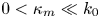 $0<\kappa _m\ll k_0$) is the maximum wavenumber of the packet resulting from the assumption of narrow bandwidth,
  $c_0$ is the phase velocity and
  $c_{g0}$ is the group velocity of the wavepacket on the deeper side.
2.4. Overall structure of the solutions and underlying physics
Before constructing explicit solutions to the problem of interest, we first explain the key components of these solutions and the underlying physics. The solutions can be described as functions of the parameters of an incident wavepacket, as detailed in §§ 2.5 and 2.6. Taking the velocity potential as an example, a flow diagram of the solution associated with an incoming wavepacket is shown in figure 2, and a summary of the expressions for the velocity potential is presented in table 1 in Appendix D. In figure 2, the velocity potential is organised according to the order of product of wave steepness and bandwidth, as explained below. Naturally, we limit the discussion to those cases in which the incident wavepacket propagating over a step ‘feels’ the abrupt depth change. That is, the water depth compared to the carrier wavelength of an incoming wavepacket is  ${O}(1)$ on at least one side of the step if not both.

Figure 2. Flow diagram of the perturbation theory solutions for the velocity potential of a narrow-banded wavepacket propagating over a step. The terms are organised according to the order of the product of wave steepness and bandwidth. From the top to the bottom row, the figure shows the incident, first-order, second-order superharmonic and second-order subharmonic or mean wavepackets. The subscripts  $I$,
$I$,  $T$ and
  $E$ denote the incoming, transmitted and evanescent wavepackets, with
  $d$ and
  $s$ used to label the evanescent wavepackets on the deeper and shallower sides, respectively. The subscripts
  $b$ and
  $f$ denote bound and free waves at second order in wave steepness, respectively. A summary of the expressions for the velocity potential is given in Appendix D.
Table 1. Solutions for different velocity potentials at  ${O}(\epsilon ^i\delta ^{\,j})$ according to the overall structure presented in § 2.4.

At first order in wave steepness, specifically  ${O}(\epsilon \delta ^0)$, an incident wavepacket responds to an abrupt depth change by being reflected (
 $\varPhi ^{(11,0)}_R$) and transmitted (
 $\varPhi ^{(11,0)}_T$), complemented by the generation of evanescent waves (
 $\varPhi ^{(11,0)}_{Ed}$ on the deeper side and
  $\varPhi ^{(11,0)}_{Es}$ on the shallower side) near the step (cf. Massel Reference Massel1983).
The mechanism that gives rise to waves at second order, namely  ${O}(\epsilon ^2)$, can be divided into two parts. The first is the forcing of bound waves by combinations of linear waves that also arises in the absence of a step (cf. (2.10f)) and is well established (Massel Reference Massel1983; Mei et al. Reference Mei, Stiassnie and Yue1989; Calvert et al. Reference Calvert, Whittaker, Raby, Taylor, Borthwick and van den Bremer2019). The second comprises the release of bound waves into free waves owing to the presence of the step. Forcing by combinations of linear waves leads to bound waves (denoted with the subscript
  $b$ in figure 2) that can only propagate together with the linear wavepacket. In contrast, free waves satisfy the linear dispersion relation and, hence, propagate independently. The bound waves include superharmonic bound waves (
 ${O}(\epsilon ^2\delta ^0)$), which are proportional to
  $\exp (2\mathrm {i}\psi )$, and subharmonic bound waves (
 ${O}(\epsilon ^2\delta ^1)$), which are independent of the rapidly varying phase
  $\psi _0$. Upon travelling over the step, these bound waves may be transmitted or reflected, staying bound, or be released into freely propagating wavepackets. In addition, new evanescent waves will be generated. The freely propagating wavepackets overlap with the linear wavepackets near the step, but will separate after a certain length of propagation owing to their different speeds. The distance over which separation occurs depends on the difference in group speeds and packet length.
2.5. First-order solutions (up to  ${O}(\epsilon \delta ^1)$)

In this section, we extend the monochromatic-wave solutions presented in Massel (Reference Massel1983) to allow for a wavepacket that varies slowly in both space and time. Following Massel (Reference Massel1983),  $\varPhi ^{(1)}$ is expressed as
 \begin{align} \varPhi^{(1)} &= {\varPhi^{(11,0)}_I+\varPhi^{(11,0)}_R+\sum_{n=1}^{\infty}\varPhi^{(11,0)}_{Ed,n}} +\delta \varPhi^{(11,1)}+{O}(\epsilon\delta^2)\quad\textrm{for}\ x<0, \end{align}
 \begin{align}\varPhi^{(1)} &= {\varPhi^{(11,0)}_T+\sum_{m=1}^{\infty}\varPhi^{(11,0)}_{Es,m}} + {\varPhi^{(11,1)}_T+\delta\varPhi^{(11,1)}}+{O}(\epsilon\delta^2)\quad\textrm{for}\ x>0, \end{align}
in which the subscripts  $I$,
$I$,  $R$ and
  $T$ denote the (propagating) incoming, reflected and transmitted wavepackets, respectively. The subscripts
  $Ed,n$ and
  $Es,m$ denote the evanescent waves on the deeper and shallower sides, respectively. As for the case without a step, one can easily show that
  $\varPhi ^{(11,1)}$ does not contribute to the second-order solutions at
  ${O}(\epsilon ^2\delta )$, but only to those at higher orders in bandwidth (see § 2.6). The details of the derivation of
  $\varPhi ^{(11,1)}$ are nevertheless included in Appendix A for completeness.
The linearised boundary value problem (2.1)–(2.5) yields
 \begin{gather} \varPhi^{(11,0)}_R =\dfrac{g}{\omega_0}\dfrac{\cosh k_0(z+h_d)}{\cosh k_0h_d}|R_0|A_R(X,T)\sin{({-}k_0x_0-\omega_0 t +\mu_0+\mu_R)} , \end{gather}
 \begin{gather}\varPhi^{(11,0)}_T =\dfrac{g}{\omega_0}\dfrac{\cosh k_{0s}(z+h_s)}{\cosh k_{0s}h_s}|T_0|A_{T}(X,T)\sin{(k_{0s}x_0-\omega_0 t + \mu_0+ \mu_T)} , \end{gather}
 \begin{gather}\varPhi^{(11,0)}_{Ed,n} = \mathcal{I} \left(\dfrac{g}{\omega_0}\dfrac{\cosh k_n(z+h_d)}{\cosh k_nh_d}R_n A_{Ed,n}(X,T) \exp({-\mathrm{i} k_nx_0-\mathrm{i}\omega_0 t+\mu_0})\right), \end{gather}
 \begin{gather}\varPhi^{(11,0)}_{Es,m} = \mathcal{I} \left(\dfrac{g}{\omega_0}\dfrac{\cosh k_m(z+h_s)}{\cosh k_mh_s}T_m A_{Es,m}(X,T) \exp({\mathrm{i} k_mx_0-\mathrm{i}\omega_0 t+\mu_0})\right), \end{gather}
where the reflection coefficient  $R_0=|R_0|\exp (\mathrm {i} \mu _R)$ and the transmission coefficient
  $T_0=|T_0|\exp (\mathrm {i} \mu _T)$ as well as the evanescent wave coefficients
  $R_n$ and
  $T_m$ are complex, and
  $\mathcal {I}$ denotes the imaginary component. The coefficients
  $R_0$,
  $R_n$,
  $T_0$ and
  $T_m$ of the free waves at
  ${O}(\epsilon \delta ^0)$ are solved for numerically based on the boundary conditions at the step described by (2.4) and (2.5):
 \begin{align}\dfrac{\cosh k_0(z+h_d)}{\cosh k_0h_d} +\sum_{n=0}^{N} R_n \dfrac{\cosh k_n(z+h_d)}{\cosh k_nh_d} &= \sum_{m=0}^{M} T_m \dfrac{\cosh k_m(z+h_s)}{\cosh k_mh_s} \nonumber\\ &\qquad \textrm{for}\ -h_s < z < 0,\end{align}
 \begin{align}\mathrm{i} k_0 \dfrac{\cosh k_0(z+h_d)}{\cosh k_0h_d} -\mathrm{i} k_n \sum_{n=0}^{N} R_n\dfrac{\cosh k_n(z+h_d)}{\cosh k_nh_d} &= \mathrm{i} k_m\sum_{j=0}^{M} T_m \dfrac{\cosh k_m(z+h_s)}{\cosh k_mh_s}\nonumber\\ &\qquad \textrm{for}\ -h_s < z < 0, \end{align}
 \begin{align}\mathrm{i} k_0 \dfrac{\cosh k_0(z+h_d)}{\cosh k_0h_d} -\mathrm{i} k_n \sum_{n=0}^{N} R_n\dfrac{\cosh k_n(z+h_d)}{ \cosh k_nh_d} &= 0\quad \textrm{for}\ -h_d < z < {-}h_s, \end{align}
where  $N$ and
  $M$ denote the finite number of evanescent modes used on the deeper and shallower sides, respectively. We show in Appendix B how
  $R_n$ and
  $T_m$ are numerically solved for using the orthogonality properties of the functions
  $\cosh k_i(z+h_d)$ and
  $\cosh k_i(z+h_s)$.
Departing from the analysis of Massel (Reference Massel1983), the packets are now allowed to vary slowly in time and space. Detailed derivations are presented in Appendix C. After taking into account the boundary conditions at the step, their dependence on time and space can be expressed as
 \begin{gather} A_R(X,T) = A_I({-}X-c_{g0}T), \quad A_{Ed,n}(X,T) = A_I({c_{g0}}X/{c_{gn}}- c_{g0}T), \end{gather}
 \begin{gather}A_T(X,T) = A_I({c_{g0}}X/{c_{g0s}}- c_{g0}T),\quad A_{Es,m}(X,T) = A_I({c_{g0}}X/{c_{gm}}- c_{g0}T), \end{gather}
where we note that these packets are continuous at  $x=0$, the packets of the reflected and transmitted packets travel at the group speed determined by the local depth and we have used analytic continuation for the spatial dependence of the evanescent wavepackets. The following relations hold for the wavenumbers and group velocities, respectively:
 \begin{gather} \omega^2_0=gk_i\tanh k_ih_d = gk_j \tanh k_j h_s, \end{gather}
 \begin{gather} c_{gi} =\left. \dfrac{\text{d}\omega}{\text{d} k}\right|_{k=k_{i}} ,\quad c_{gj} =\left. \dfrac{\text{d}\omega}{\text{d} k}\right|_{k=k_{j}}, \end{gather}
where  $i = {0}$ or
  ${n}$,
  $j = {0s}$ or
  ${m}$,
  $k_0$ and
  $k_{0s}$ are real wavenumbers, and the rest of the wavenumbers and corresponding group speeds are imaginary. The imaginary wavenumbers correspond to evanescent waves that vanish with horizontal distance away from the step, as
  $\exp (-|\mathrm {i} k_n x|)$ or
  $\exp (-|\mathrm {i} k_m x|)$.
2.6. Second-order solutions $({O}(\epsilon ^2))$

The free-surface boundary conditions can be combined into one, which gives at  ${O}(\epsilon ^2)$ (e.g. Longuet-Higgins & Stewart Reference Longuet-Higgins and Stewart1964; McAllister et al. Reference McAllister, Adcock, Taylor and van den Bremer2018)
 \begin{align} \dfrac{\partial^2 \varPhi^{(2)}}{\partial t^2} + g \dfrac{\partial \varPhi^{(2)}}{\partial z} &={-} \frac{\partial}{\partial t} \left[ \frac{1}{2}\left(\dfrac{\partial \varPhi^{(1)}}{\partial x} \right)^2+ \frac{1}{2}\left(\dfrac{\partial \varPhi^{(1)}}{\partial z} \right)^2 + \zeta^{(1)}\frac{\partial^2 \varPhi^{(1)}}{\partial z\partial t} \right] \nonumber\\ &\quad + g \dfrac{\partial}{\partial x} \left( \frac{\partial \varPhi^{(1)}}{\partial x}\zeta^{(1)}\right) \quad \text{at}\ z=0,~ \end{align}
with a corresponding diagnostic equation for the surface elevation at  ${O}(\epsilon ^2)$
 \begin{equation} \zeta^{(2)} ={-}\dfrac{1}{g}\left(\dfrac{\partial \varPhi^{(2)}}{\partial t} + \dfrac{1}{2} \left(\boldsymbol{\nabla}\varPhi^{(1)} \right)^2+\dfrac{\partial^2 \varPhi^{(1)}}{\partial t\partial z}\zeta^{(1)}\right), \end{equation}
in which the second term on the right-hand side becomes zero in deep water.
Substituting the linear solutions (2.11) into (2.17) and collecting terms at  ${O}(\epsilon ^2)$ yields
 \begin{equation} \dfrac{\partial^2 \varPhi^{(2)}}{\partial t^2} + g \dfrac{\partial \varPhi^{(2)}}{\partial z} = \delta^0 F_{\epsilon^2\delta^0} +\delta F_{{\epsilon^2\delta^1}} +{O}(\epsilon^2\delta^2) \end{equation}
with
 \begin{align} F_{\epsilon^2\delta^0} &={-} \frac{\partial}{\partial {t_0}}\left[\frac{1}{2}\left(\dfrac{\partial \varPhi^{(11,0)}}{\partial {x_0}} \right)^2+ \frac{1}{2}\left(\dfrac{\partial \varPhi^{(11,0)}}{\partial z} \right)^2 + \zeta^{(11,0)}\frac{\partial^2 \varPhi^{(11,0)}}{\partial z\partial {t_0}}\right] \nonumber\\ &\quad + g\dfrac{\partial}{\partial {x_0}} \left( \frac{\partial \varPhi^{(11,0)}}{\partial {x_0}}\zeta^{(11,0)}\right), \end{align}
 \begin{align} F_{\epsilon^2\delta^1} &={-} \frac{\partial}{\partial {T}} \left[ \frac{1}{2}\left(\dfrac{\partial \varPhi^{(11,0)}}{\partial {x_0}} \right)^2+ \frac{1}{2}\left(\dfrac{\partial \varPhi^{(11,0)}}{\partial z} \right)^2 + \zeta^{(11,0)}\frac{\partial^2 \varPhi^{(11,0)}}{\partial z\partial {t_0}}\right]\nonumber\\ &\quad - \frac{\partial}{\partial {t_0}} \left[ \dfrac{\partial \varPhi^{(11,0)}}{\partial {x_0}} \left( \dfrac{\partial \varPhi^{(11,0)}}{\partial {X}}+ \dfrac{\partial \varPhi^{(11,1)}}{\partial {x_0}}\right) + \dfrac{\partial \varPhi^{(11,0)}}{\partial {z}} \dfrac{\partial \varPhi^{(11,1)}}{\partial {z}}\right]\nonumber\\ &\quad +\frac{\partial}{\partial {t_0}} \left( \zeta^{(11,1)}\frac{\partial^2 \varPhi^{(11,0)}}{\partial z\partial {t_0}} + \zeta^{(11,0)}\frac{\partial^2 \varPhi^{(11,1)}}{\partial z\partial {t_0}} \right) \nonumber\\ &\quad + g \dfrac{\partial}{\partial {X}} \left(\frac{\partial \varPhi^{(11,0)}}{\partial {x_0}}\zeta^{(11,0)}\right) + g \dfrac{\partial}{\partial {x_0}} \left(\zeta^{(11,1)}\frac{\partial \varPhi^{(11,0)}}{\partial {x_0}} + \zeta^{(11,0)}\frac{\partial \varPhi^{(11,1)}}{\partial {x_0}} \right), \end{align}
in which  $F_{\epsilon ^2\delta ^0}$ and
  $F_{\epsilon ^2\delta ^1}$ can be further decomposed based on wave harmonics. A similar equation can be obtained for
  $\zeta ^{(2)}$ (not shown).
After identifying the harmonics of the forcing terms  $F_{\epsilon ^2\delta ^0}$ and
  $F_{\epsilon ^2\delta ^1}$, the second-order solutions of
  $\varPhi ^{(2)}$ and
  $\zeta ^{(2)}$ can be separated into two parts with different harmonics:
 \begin{gather} \varPhi^{(2)} = \varPhi^{(22,0)} + \delta \varPhi^{(20,1)}, \end{gather}
 \begin{gather}\zeta^{(2)}= \zeta^{(22,0)}+\delta \zeta^{(20,1)}, \end{gather}
in which  $\varPhi ^{(22,0)}$ and
  $\zeta ^{(22,0)}$ are the superharmonic terms proportional to
  $\exp {(-2\mathrm {i}\omega _0t_0)}$ and
  $\varPhi ^{(20,1)}$ and
  $\zeta ^{(20,1)}$ are the subharmonic (or mean) terms that are independent of fast time
  $t_0$.
2.6.1. Superharmonic packets at ${O}(\epsilon ^2\delta ^0)$

Similar to Massel (Reference Massel1983), we seek solutions for the superharmonic packets at  ${O}(\epsilon ^2\delta ^0)$ of the form
 \begin{gather} \varPhi^{(22,0)} = \varPhi^{(22,0)}_I + \varPhi^{(22,0)}_{R,b} + \varPhi^{(22,0)}_{R,f} + \mathcal{I}\left(\sum_{n=1}\varPhi^{(22,0)}_{Ed,n}\right)\quad\text{for}\ x<0, \end{gather}
 \begin{gather}\varPhi^{(22,0)} = \varPhi^{(22,0)}_{T,b} + \varPhi^{(22,0)}_{T,f} +\mathcal{I}\left( \sum_{m=1}\varPhi^{(22,0)}_{Es,m}\right)\quad\text{for}\ x>0, \end{gather}
in which subscripts  $b$ and
  $f$ denote superharmonic bound and free waves, respectively. In order to obtain tractable solutions, we ignore forcing by product linear evanescent waves, which are typically small. We justify this assumption ex post by comparing with fully nonlinear numerical simulations. We note that inclusion of forcing by evanescent terms can lead to convergence problems of second-order solutions (Monsalve Gutiérrez Reference Monsalve Gutiérrez2017). After considerable manipulation, we obtain
 \begin{gather} \varPhi^{(22,0)}_{R,b} = \dfrac{3\omega_0}{8}|R_0|^2A^2_R\dfrac{\cosh 2k_0(z+h_d)}{\sinh^4 k_0 h_d} \sin({-}2k_0x-2\omega_0 t + 2\mu_0 +2\mu_R), \end{gather}
 \begin{gather}\varPhi^{(22,0)}_{R,f} = \omega_0|R_{20}|A^2_I\left(-\dfrac{c_{g0}}{c_{g20}}X-c_{g0}T\right)\dfrac{\cosh k_{20}(z+h_d)}{\cosh k_{20} h_d} \sin({-}k_{20}x-2\omega_0 t + 2\mu_0+ \mu_{20}), \end{gather}
 \begin{gather}\varPhi^{(22,0)}_{Ed,n} = \omega_0 R_{2n} A^2_I\left(-\dfrac{c_{g0}}{c_{g2n}}X-c_{g0}T\right)\dfrac{\cosh k_{2n}(z+h_d)}{\cosh k_{2n} h_d} \exp(-\mathrm{i} (k_{20}x+2\omega_0 t) + 2\mu_0), \end{gather}
 \begin{gather}\varPhi^{(22,0)}_{T,b} = \dfrac{3\omega_0}{8}|T_0|^2A^2_I\left(\dfrac{c_{g0}}{c_{g0s}}X-c_{g0}T\right)\dfrac{\cosh 2k_{0s}(z+h_s)}{\sinh^4 k_{0s} h_s} \sin(2k_{0s}x-2\omega_{0s} t + 2\mu_0 + 2\mu_T), \end{gather}
 \begin{gather}\varPhi^{(22,0)}_{T,f} = \omega_0 |T_{20}|A^2_I\left(\dfrac{c_{g0}}{c_{g20s}}X-c_{g0}T\right)\dfrac{\cosh k_{20s}(z+h_s)}{\cosh k_{20s} h_s}\sin(k_{20s}x-2\omega_0 t + 2\mu_0+ \mu_{20s}), \end{gather}
 \begin{gather}\varPhi^{(22,0)}_{Es,m}= \omega_0 T_{2m} A^2_I\left(\dfrac{c_{g0}}{c_{g2m}}X-c_{g0}T\right) \dfrac{\cosh k_{2m}(z+h_s)}{\cosh k_{2m} h_s} \exp(-\mathrm{i} (k_{2m}x-2\omega_0 t + 2\mu_0)) , \end{gather}
 \begin{gather}4\omega_0^2 = g k_{2i} \tanh (k_{2i}h_d)\quad \textrm{for}\ i=0, 1, 2, 3,\ldots, \end{gather}
 \begin{gather}4\omega_0^2 = g k_{2j} \tanh (k_{2j} h_s)\quad \textrm{for}\ j=0s, 1, 2, 3,\ldots, \end{gather}
where the last two equations denote the dispersion relationships associated with the frequency  $2\omega _0$ for two different depths
  $h_d$ and
  $h_s$. The wavenumbers
  $k_{20}$ and
  $k_{20s}$ are real, and the other superharmonic wavenumbers are imaginary and correspond to evanescent waves. The reflection (
 $R_{2n}$) and transmission (
 $T_{2m}$) coefficients are solved for numerically from the boundary conditions at the step (2.4) and (2.5) at this particular order. The group velocities and the phases are defined as
 \begin{gather} c_{g2i} = \dfrac{\omega_0}{k_{2i}}\left(1+\dfrac{2k_{2i}h_j}{\sinh(2k_{2i}h_j)}\right), \end{gather}
 \begin{gather}\psi_{20} = \text{arg}(R_{20}),\quad \psi_{20s} = \text{arg}(T_{20}). \end{gather}
in which  $k_{2i}h_j = k_{2i}h_d$ (
 $i=0,1,2,\ldots$) or
  $k_{2i}h_j = k_{2i}h_s$ (
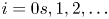 $i=0s,1,2,\ldots$).
2.6.2. Subharmonic packets at ${O}(\epsilon ^2\delta ^1)$

In this section, we present second-order subharmonic solutions, which were not included by Massel (Reference Massel1983). Averaging in time over the fast scales, we find that  $F_{\epsilon ^2\delta ^0}=0$. The solutions at
  ${O}(\epsilon \delta )$ do not contribute to leading order, and we obtain the following for the subharmonic forcing at second order:
 \begin{gather} \overline{F_{\epsilon^2\delta^0}+\delta F_{\epsilon^2\delta^1}}={-} \delta \dfrac{g^2}{\omega^2_0}\frac{\partial}{\partial {T}}\left[\frac{k_0^2}{4}(1- \tanh^2k_0h_d)(A_I^2+A_R^2)\right] \nonumber\\ \hspace{5.3pc}+\,\delta \dfrac{g^2}{2\omega_0} \frac{\partial}{\partial {X}} [k_0(A_I^2-A_R^2)] \quad \text{for}\ X<0, \end{gather}
 \begin{gather} \overline{F_{\epsilon^2\delta^0}+\delta F_{\epsilon^2\delta^1}}={-} \delta \dfrac{g\omega_0}{2c_{g0s}\tanh k_{0s}h_s} \left[\dfrac{c_{g0s}}{2c_{0s}}(1-\tanh^2k_{0s}h_s)+1\right]\partial_T(A_T^2)\quad \text{for}\ X>0, \end{gather}
where  $c_{0s}=\omega _0/k_{0s}$ denotes the phase velocity of the linear carrier wave on the shallower side. In order to maintain tractable solutions, we ignore forcing by linear evanescent waves. As for the second-order superharmonic solutions, we justify this assumption ex post by comparing with fully nonlinear numerical simulations.
The forcing in (2.27), together with the Laplace equation (2.1) and the bottom boundary condition (2.3), leads to the following subharmonic bound waves:
 \begin{align} \varPhi^{(20,1)}_b(X,T,z) &= \varPhi_I^{(20,1)} + B_R {\int\limits_{-\varOmega_m}^{\varOmega_m}} \dfrac{\mathrm{i}\kappa g\omega_0\hat{E}_R(\varOmega)}{g\kappa_0\tanh \delta \kappa_0 h_d-\delta \varOmega^2} \dfrac{\cosh \delta \kappa_0(z+h_d)}{\cosh \delta \kappa_0 h_d}\, \mathrm{e}^{-\mathrm{i} \varOmega T}\,\mathrm{d} \varOmega \nonumber\\ &\qquad\text{for}\ X<0,\end{align}
 \begin{align} \varPhi^{(20,1)}_b(X,T,z) &= B_T{\int\limits_{-\varOmega_m}^{\varOmega_m} \dfrac{\mathrm{i} {\kappa_{0s}} g \omega_0\hat{E}_T({\varOmega})}{g{\kappa_{0s}}\tanh\delta{\kappa_{0s}} h_s-\delta \varOmega^2} } \dfrac{\cosh \delta \kappa_{0s}(z+h_s)}{\cosh \delta \kappa_{0s} h_s}\,\mathrm{e}^{-\mathrm{i} \varOmega T}\,\mathrm{d} \varOmega \nonumber\\ &\qquad \text{for}\ X>0, \end{align}
where 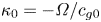 $\kappa _0 = -\varOmega /c_{g0}$,
 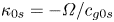 $\kappa _{0s} = -\varOmega /c_{g0s}$,
  $\varOmega _m$ (
 $0<\delta \varOmega _m\ll \omega _0$) is the maximum frequency of the packet resulting from the assumption of narrow bandwidth and
 \begin{gather} \hat{E}_R(\varOmega) = \dfrac{1}{4{\rm \pi}} \int\limits^{\infty}_{-\infty} R_0^2A_R^2\, \mathrm{e}^{\mathrm{i}\varOmega T}\,\mathrm{d} T, \quad \hat{E}_T{(\varOmega)} = \dfrac{1}{4{\rm \pi}} \int\limits^{\infty}_{-\infty} T_0^2A_T^2\,\mathrm{e}^{\mathrm{i}\varOmega T}\,\mathrm{d} T, \end{gather}
 \begin{gather}B_R ={-} \dfrac{1}{\tanh k_0h_d} \left[\dfrac{c_{g0}}{2c_0}(1-\tanh^2k_0h_d)-1\right], \end{gather}
 \begin{gather}B_T = \dfrac{1}{\tanh k_{0s}h_s} \left[\dfrac{c_{g0s}}{2c_{0s}}(1-\tanh^2k_{0s}h_s)+1\right]. \end{gather}
The bound subharmonic waves in (2.28) correspond to those of the incoming, reflected and transmitted separately. Together, these bound waves do not satisfy the boundary conditions at the step, where additional free waves are generated. To avoid prohibitively cumbersome solutions, we make the additional assumption that the subharmonic packet is long relative to the water depth, so that the mean flow is shallow (see Calvert et al. Reference Calvert, Whittaker, Raby, Taylor, Borthwick and van den Bremer2019). This assumption covers most practical applications in coastal waters.
2.6.3. The long-wave approximation for subharmonic packets ($1/(kh\delta ) \gg 1$)

In the limit  $1/(kh\delta ) \gg 1$ for both
  $h_d$ and
  $h_s$, but for
  $k_0 h_d={O}(1)$ and
  $k_{0s} h_s={O}(1)$, the bound subharmonic behaviour can be described in terms of horizontal velocities
 \begin{equation} u^{(20,1)}_{I} = \dfrac{g k_0 B_d}{c_{g0}}A_I^2,\quad u^{(20,1)}_{R,b} ={-} \dfrac{g k_0|R_0|^2 B_d}{c_{g0}}A_R^2,\quad u^{(20,1)}_{T,b} =\dfrac{g k_{0s}|T_0|^2 B_s }{c_{g0s}} A_T^2, \end{equation}
and mean set-downs of the surface elevation
 \begin{equation} \zeta^{(20,1)}_{I} =k_0 B_d A_I^2, \quad \zeta^{(20,1)}_{R,b} =k_0B_d |R_0|^2 A_R^2,\quad \zeta^{(20,1)}_{T,b} =k_{0s} B_s |T_0|^2 A_T^2, \end{equation}
where the non-dimensional coefficients  $B_d$ and
  $B_s$ are given by
 \begin{gather} B_d ={-}\dfrac{1}{4 (g h_d- {c}_{g0}^2 )} \left(\dfrac{2gh_d - {c}_{g0} ^2 }{2 \sinh 2k_0h_d} +\dfrac{2g c_{g0} }{\omega_0} \right) , \end{gather}
 \begin{gather}B_s ={-} \dfrac{1}{4 (g h_s- {c}_{g0s}^2 )} \left(\dfrac{2gh_s - {c}_{g0s} ^2 }{2\sinh 2k_{0s}h_s} +\dfrac{2g c_{g0s} }{\omega_0} \right). \end{gather}
When the carrier waves are additionally assumed to travel in deep water (i.e.  $k_0h_d \gg 1$ and
  $k_{0s}h_s\gg 1$) then the first term in the brackets of both (2.32a) and (2.32b) vanishes. For completeness, we note that, owing to limit
  $h/\sigma \to 0$, the order of the solutions in
  $\delta$ has increased by one, although we do not update our notation to reflect this.
In accordance with the long-wave approximation for the subharmonic packets, freely travelling subharmonic packets generated at the step propagate at the shallow-water velocity, i.e.  $\sqrt {gh_d}$ on the deeper side and
  $\sqrt {gh_s}$ on the shallower side. Assuming such free subharmonic packets can propagate in both directions, we seek solutions of the form
 \begin{gather} \zeta^{(20,1)}_{R,f} = B_R^f k_0 A^2_I\left(-\frac{c_{g0}}{\sqrt{gh_d}}X-c_{g0}T\right), \quad \zeta^{(20,1)}_{T,f} = B_T^f k_{0s}A^2_I\left(\frac{c_{g0}}{\sqrt{gh_s}}X-c_{g0}T\right), \end{gather}
 \begin{gather} u^{(20,1)}_{R,f} ={-} \sqrt{\frac{g}{h_d}}B_R^f k_{0} A^2_I\left(-\frac{c_{g0}}{\sqrt{gh_d}}X-c_{g0}T\right), \quad u^{(20,1)}_{T,f} = \sqrt{\frac{g}{h_s}}B_T^f k_{0s} A^2_I\left(\frac{c_{g0}}{\sqrt{gh_s}}X-c_{g0}T\right). \end{gather}
The relationship between  $u$ and
  $\zeta$ is set by
  $\partial _t u = -g \partial _x \zeta$ (cf. (4.1.3) in Mei et al. (Reference Mei, Stiassnie and Yue1989)). The coefficients
  $B_R^{f}$ and
  $B_T^{f}$ must be found from the matching conditions at the step. For a shallow flow (see e.g. Mei et al. (Reference Mei, Stiassnie and Yue1989) for details), these become (i) continuity of the volume flux across the step and (ii) continuity of the free surface across the step:
 \begin{equation} \lim_{X\to0^-}u^{(20,1)} h_d = \lim_{X\to0^+}u^{(20,1)} h_s,\quad\lim_{X\to0^-}\zeta^{(20,1)} =\lim_{X\to0^+}\zeta^{(20,1)}, \end{equation}
where we note that  $u^{(1)}(z=0)\eta ^{(1)}$ from depth integration of the linear velocity truncated at second order is not included in (2.34a), as this is already continuous across the step. Hence, we obtain
 \begin{gather} B_{T}^f = \dfrac{gk_{0s}h_sB_s|T_0|^2/c_{g0s} + gk_{0}h_dB_d(1-|R_0|^2)/c_{g0}+ \sqrt{gh_d} (k_{0s}B_s|T_0|^2 - k_{0}B_d(|R_0|^2+1))} {(\sqrt{gh_d}+\sqrt{gh_s})k_{0s}}, \end{gather}
 \begin{gather}B_{R}^f = \dfrac{gk_{0s}h_sB_s|T_0|^2/c_{g0s} - gk_{0}h_dB_d(1-|R_0|^2)/c_{g0} - \sqrt{gh_s} (k_{0s}B_s|T_0|^2 - k_{0}B_d(|R_0|^2+1))} {(-\sqrt{gh_d}-\sqrt{gh_s})k_{0}}. \end{gather}
We note that the relations  $\text {sign}(B_T^f) = - \text {sign}(B_s)$ and
  $\text {sign}(B_R^f) = - \text {sign}(B_s)$ hold, and both free waves are thus positive, taking the form of set-ups, as the sign of the bound set-down is always negative. The coefficients
  $B_{T}^f$ and
  $B_{T}^f$ only depend on two non-dimensional parameters:
  $k_0h_d$ and
  $k_0h_s$. We further explore these solutions and the underlying physics in the next section.
3. Results
In order to examine the predictions of the theoretical model in § 2, we consider an incoming Gaussian wavepacket on the deeper side defined as follows:
 \begin{equation} \zeta^{(11,0)}_I = A_0 \exp\left(-\dfrac{(x-x_\text{f} - c_{g0}(t-t_{f}))^2}{2\sigma^2_x}\right )\cos(k_0x - \omega_0t), \end{equation}
in which  $k_0$ and
  $\omega _0$ are the carrier wavenumber and angular frequency, respectively,
  $c_{g0} = \omega _0 /(2k_0) (1+2k_0h_d/\sinh (2k_0h_d))$ is the group velocity on the deeper side,
  $\sigma _x$ is the characteristic length of the packet, and
  $x_{f}$ denotes the location where the linear irregular waves focus at time
  $t_{f}$. We set the wave steepness
  $\epsilon = k_0A_0=0.03$ and the bandwidth parameter
  $\delta = 1/(k_0\sigma _x)=0.06$, so that both remain much smaller than
  $1$ in accordance with the assumptions presented in § 2.
We examine three distinct stages of evolution: stage I when the packet is sufficiently far ahead of the step on the deeper side, stage II when the packet ‘feels’ the step and transient processes in the vicinity of the step take place and stage III when the packet has left the step behind.
3.1. Generation of free packets: stage I versus stage III
Figure 3 shows the theoretically predicted free-surface elevation before (stage I) and after (stage III) passing the step. Before the step ( figure 3a–d), the main (linear) packet is associated with an in-phase superharmonic bound wavepacket and a subharmonic bound set-down (cf. (2.10f)), as is well known (e.g. Mei et al. Reference Mei, Stiassnie and Yue1989; Calvert et al. Reference Calvert, Whittaker, Raby, Taylor, Borthwick and van den Bremer2019). After the step ( figure 3e–h), both the superharmonic bound wavepacket and the subharmonic bound set-down have increased in magnitude. Also present are two additional superharmonic wavepackets and two additional subharmonic components, only one of which is visible in figure 3.

Figure 3. Theoretically predicted interaction with a step decomposed by order and phase, showing stage I before the step (a–d) and stage III after the step (e–h). In the figure,  $\epsilon = 0.03$,
  $\delta = 0.06$,
  $k_0h_d = 1.1$,
  $k_{0s}h_s = 0.70$,
  $h_d = 0.75$ m,
  $h_s/h_d = 0.53$,
  $T_{{p}} = 1.9$ s is the carrier wave period and
  $\lambda _0 = 4.4$ m. The step is located at
  $x = 0$. Panels (a–d) correspond to
  $t = 30 T_p$ before the main wavepacket reaches the step and (e–f) to
  $t = 70 T_p$ after it has passed the step.
The response to the step is most clearly illustrated in figure 4. Focusing on figure 4(a) first, the bound superharmonic wavepacket on the deeper side is split into three wavepackets after experiencing the depth transition, one of which stays bound and travels with the main packet at  $c_{g0s}$. A first additional superharmonic free wavepacket propagates in the same direction as the main packet, but slower at
  $c_{g20}$ (
 $c_{g20s} < c_{g0s}$). A second additional superharmonic free wavepacket propagates and is reflected and travels in the opposite direction at an absolute speed of
  $c_{g20}$ (
 $c_{g20} < c_{g0}$).

Figure 4. Theoretically predicted spatio-temporal evolution of superharmonic (a) and subharmonic (b) wavepackets following interaction with a step at  $x=0$. The parameters are the same as in figure 3. The straight red lines with arrowheads indicate the different group speeds and their propagation directions.
Analogous behaviour is observed in figure 4(b), except that the subharmonic free components are shallow-water waves and travel at higher speeds than the main (linear) packet. The subharmonic bound wave, manifest as a set-down of the free surface, becomes deeper on the shallower side. A free subharmonic set-up is released that propagates at the shallow-water speed  $\sqrt {gh_s}$ in the direction of the main packet but faster. A free subharmonic set-down is reflected and travels in the opposite direction to the main packet at an absolute speed
  $\sqrt {gh_d}$ on the deeper side.
3.2. Amplitudes change and phases shift due to an abrupt depth transition
In the previous section, we examined a single combination of parameters. Although the four additional free second-order components will be generated for any combination of parameters, their amplitudes and phases depend on two dimensionless parameters, the relative depth on the deeper side  $k_0h_d$ and the depth ratio
  $h_d/h_s$, in addition to the steepness squared. The linear reflection and transmission coefficients
  $R_0$ and
  $T_0$ are computed based on (2.13). The reflection and transmission coefficients for the superharmonic free wavepackets
  $R_{20}$ and
  $T_{20}$ are computed from the boundary conditions at the step in a similar fashion to (2.13). The reflection and transmission coefficients for the subharmonic free components
  $B_R^f$ and
  $B_T^f$ are given explicitly in (2.34a,b). The magnitudes and phases of all these coefficients are shown as functions of the two non-dimensional parameters in figure 5.

Figure 5. Contours of amplitudes and phases of the theoretically predicted reflection and transmission coefficients as functions of  $k_0h_d$ and the depth ratio
  $h_s/h_d$.
Examining first the coefficients for the first harmonic shown in figure 5(a–d) (see also Massel Reference Massel1983), the transmitted waves are amplified for  $k_0h_d \lesssim 2.0$. The coefficient of reflection can reach a maximum of
  $\sim 30\,\%$ when the depth ratio decreases to
  $0.3$. Figure 5(b,d) shows that, relative to the incoming wavepacket, the transmitted linear waves generally have small phase shifts (
 ${\lesssim }0.05{\rm \pi}$) and the reflected waves have a phase shift
  ${\lesssim }0.2{\rm \pi}$ when their amplitudes are
  ${\sim }10\,\%$–
 $30\,\%$ of the incoming wavepacket (comparing figures 5a and 5b).
Figure 5(e, f,i,j) shows the reflection and transmission coefficients of the free superharmonic waves. These are generally largest in magnitude for small  $k_0 h_d$ and small depth ratios
  $h_s/h_d$ with the transmitted component considerably larger than the reflected component. Relative to the incoming wavepacket, the reflected superharmonic waves show small phase shifts, whereas the transmitted waves have a phase shift of between
  $-0.9{\rm \pi}$ and
  $-{\rm \pi}$. The latter is the cause of local transient maxima in crest elevation occurring in the vicinity of the step, as we examine in § 3.3.
The coefficients for the reflected and transmitted free and bound subharmonic components are calculated based on the long-wave approximation for these components presented in § 2.6.3 and shown in figure 5(g,h,k,l). The reflected free subharmonic components travel backwards on the deeper side in the form of a set-down, whereas the transmitted free subharmonic components travel forwards on the shallower side in the form of a set-up. We emphasise that the coefficients presented in figure 5 need to be used with care for small  $k_0 h_s$, as a Stokes expansion is likely no longer valid for very shallow depths.
3.3. Behaviour near the abrupt depth transition: stage II
As noted in § 3.2, the transmitted superharmonic free wavepacket has a phase shift of approximately  ${\rm \pi}$ relative to the transmitted main wavepacket (and its in-phase bound superharmonics). As a result of the smaller group velocity, the superharmonic and the transmitted main packet temporarily overlap just after the step before separating. These processes can be associated with two characteristic length scales: a beating length
  $L_b$ and an overlapping length
  $L_o$. Beating occurs when the free and bound superharmonic waves are in phase, namely at
  $x=L_b$ and
 \begin{equation} L_b(n)=\dfrac{-\arg(T_{20})+2\arg(T_{0})+2{\rm \pi} (n-1)}{k_{20s}-2k_{0s}}, \end{equation}
for any positive integer  $n$ with the first beat corresponding to
  $n=1$, noting that
  $\arg (T_{0})\approx 0$ and
  $\arg (T_{2})\approx -{\rm \pi}$. Taking
  $4\sigma _{x,s}$ with
  $\sigma _{x,s}=\sigma _x c_{g0s}/c_{g0}$ as an estimate of the length of the group, the two groups will no longer overlap at
  $x=L_o$ and
 \begin{equation} L_o=\dfrac{4\sigma_{x,s}}{1-c_{g20s}/c_{g0s}}, \end{equation}
which denotes the distance between the peak of the main wavepacket and the step when the two groups just separate.
As the envelopes of the superharmonic bound and the superharmonic free waves travel at different group speeds and the lengths of the packets are limited, observation of  $n$ beats requires
  $L_b(n)\leqslant L_o$. Hence, only the first (few) beat(s) will be observed. The length scales
  $L_o$ and
  $L_b(n)$ scaled by the carrier wavelength on the shallower side
  $\lambda _{0,s}$ are shown in figure 6 as a function of the dimensionless depth
  $k_{0s}h_s$. We can observe from figure 6(a) that the length for the first beat increases rapidly as the shallower water depth
  $k_{0s}h_s$ decreases for
  $k_{0s}h_s\lesssim 1.5$. At least one beat can be expected for
  $k_{0s}h_s>0.2$ and
 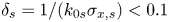 $\delta _{s}=1/(k_{0s}\sigma _{x,s})<0.1$, as shown in figure 6(b). As the group length increases (i.e.
  $\delta _{s}$ decreases), more beats can be expected. When we eventually approach to the limit
  $\delta _{s} \to 0$ (not shown here), denoting a uniform Stokes wave as studied and examined in Massel (Reference Massel1983), there are an infinite number of beats.

Figure 6. (a) The beating length ( $L_b(n)$ for
  $n=1$) and (b) the overlapping and beating length (
 $L_o$ and
  $L_b(n)$ for
  $n\geqslant 1$) as a function of
  $k_{0s}h_s$. In the figure,
  $\lambda _{0,s} = 2{\rm \pi} /k_{0s}$ is the carrier wavelength of the main packet on the shallower side;
 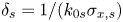 $\delta _s = 1/(k_{0s}\sigma _{x,s})$ denotes the non-dimensional bandwidth on the shallower side.
4. Numerical validation
4.1. A fully nonlinear potential-flow numerical solver
In order to validate our solutions and justify our assumption that evanescent waves do not contribute meaningfully to behaviour at second order in steepness when waves travel over a step, we perform fully nonlinear potential-flow simulations. We employ a fully nonlinear potential-flow numerical solver that uses the boundary element method for the boundary value problem described by (2.1)–(2.5). The resulting numerical wave tank was first developed by Koo & Kim (Reference Koo and Kim2004) and has recently been used to examine a related problem by Zheng et al. (Reference Zheng, Lin, Li, Adcock, Li and van den Bremer2020). Generation of waves in this numerical wave tank is based on linear theory (Havelock Reference Havelock1929), consistent with our experiments reported on in the companion paper (Li et al. Reference Li, Draycott, Adcock and van den Bremer2021).
4.2. Comparison between theory and numerical simulations
Although we have tested a number of different cases, we show a comparison here between theory and numerical simulations for the same parameters as examined in the previous section, namely  $\epsilon = 0.03$,
  $\delta = 0.06$,
  $k_0h_d = 1.1$,
  $k_{0s}h_s = 0.70$,
  $h_d = 0.75$ m,
  $h_s/h_d = 0.53$,
  $T_p = 1.9$ s and
  $\lambda _0 = 4.4$ m, which denotes the carrier wavelength on the deeper side. We choose a Gaussian wavepacket that focuses linearly at
  $t_{f} = 30T_p$ and
  $x_{{f}}=-5\lambda _0$ with the step at
  $x=0$. A computational domain of a length equal to
  $100\lambda _0$ was chosen in the numerical wave tank, where the distances between the wavemaker and the step and between the damping zone (the beach) are equal to
  $20\lambda _0$ and
  $80\lambda _0$, respectively. In order to compare the theoretical and numerical solutions explicitly for each order and phase (sub- and superharmonic), we filter the (narrow-banded) numerical solutions in the frequency domain.
Figure 7, which shows a comparison of the theoretically and numerically predicted surface elevations near the step decomposed by order and harmonic, reveals almost perfect agreement for the first-order and the second-order superharmonic and subharmonic surface elevation. The agreement includes phase and amplitude in the vicinity of the step. Figure 8 confirms this good agreement in Fourier space and figure 9 in physical space. The agreement becomes less perfect in the long-time tail of the wavepackets in figure 7, reflecting the non-dispersive approximation made in our theoretical solutions owing to truncation in bandwidth and nonlinearity (cf. Tayfun Reference Tayfun1980, Reference Tayfun1986; Mei et al. Reference Mei, Stiassnie and Yue1989; Trulsen & Dysthe Reference Trulsen and Dysthe1996). The almost negligible difference between the theory and numerical simulations shown in figure 7(i) is due to the long-packet approximation we made in § 2.6.3.

Figure 7. Comparison of the theoretically and numerically predicted interaction with the step decomposed by order. The wavepacket focuses linearly at  $t= 30 T_p$ and
  $x=-5\lambda _0$ with the step at
  $x=0$. The three different times (
 $t= 30 T_p$,
  $35T_p$,
  $40T_p$) corresponding to the three columns capture the passing of the step.

Figure 8. Comparison of the theoretically and numerically predicted free-surface elevation in Fourier wavenumber space ( $k$) at different times (a–c) and in frequency space (
 $f$) at different locations (d–f). The parameters are the same as in figure 7.

Figure 9. Comparison of the theoretically (red dashed lines) and numerically (black solid lines) predicted spatio-temporal evolution of superharmonic (a) and subharmonic (b) wavepackets following interaction with a step at  $x=0$ (vertical dashed line). The parameters are the same as in figure 7. The straight blue lines with arrowheads indicate the different group speeds and their propagation directions. The numerical results are represented by solid black lines and theory by dashed red lines.
5. Conclusions
This paper has examined the interaction of deterministic surface gravity wavepackets with an abrupt depth transition in the form of a step in intermediate water depth. To do so, we have developed second-order theory for narrow-banded wavepackets based on a Stokes and multiple-scales expansion, thereby extending the work of Massel (Reference Massel1983), which is only valid for monochromatic waves. To obtain tractable solutions from perturbation theory, we additionally assume that forcing of second-order terms due to local first-order evanescent waves, which are generated at first order owing to the presence of the step and vanish rapidly with distance away from it, can be ignored. We justify this assumption ex post by performing numerical simulations using a fully nonlinear potential-flow solver. Good agreement with our theoretical solutions is found.
As a wavepacket travels over a sudden depth transition, additional wavepackets are generated that propagate freely obeying the linear dispersion relation and arise at both first and second order in wave steepness in a Stokes expansion. As the superharmonic bound waves travel over the step, their magnitude changes, and two freely travelling superharmonic wavepackets are released. The two free packets consist of a generally in-phase reflected packet that travels in the opposite direction, and a generally out-of-phase transmitted packet propagating in the same direction as the main (linear) packet albeit at a lower speed. The same happens for the subharmonic components. In the subharmonic shallow-water limit, in which the packet is long relative to the water depth, we can find solutions for the subharmonic components in closed form. At the subharmonic level, the bound set-down generally increases in magnitude, and a free transmitted set-up travels ahead of the main packet with a free set-down being reflected.
In the region near the top of a depth transition, the resulting transient processes play a crucial role. In intermediate water depths, these processes are generally dominated by the superharmonic terms. Both the superharmonic bound waves and the freely travelling superharmonic waves appear immediately after the step on the shallower side. This causes beating, which is modulated by the envelopes of both packets and only exists near the step. Together, these effects cause a series of local peaks in surface elevation, which decline in magnitude with distance away from the step, declining more strongly for less narrow-banded and thus spatially shorter wavepackets. Such a decline is absent in the spatially periodic beating pattern predicted by Massel (Reference Massel1983) for monochromatic waves. We conjecture that this combination of beating between the bound and free superharmonic waves and modulation by their respective envelopes with each travelling at a different speed is the cause of the local peak in skewness and kurtosis near a depth transition reported in a series of previous papers reviewed in Trulsen et al. (Reference Trulsen, Raustøl, Jorde and Rye2020).
Acknowledgements
Y.Z. and Z.L. acknowledge support from the National Natural Science Foundation of China (51979162). T.S.v.d.B. acknowledges a Royal Academy of Engineering Research Fellowship. The authors thank Dr E.M. Gutierrez for sharing his code and Professor S. Liao for valuable discussions.
Funding
This work has been supported by NSFC-EPSRC-NERC grants 51479114 and EP/R007632/1. Y.L. acknowledges support from the Research Council of Norway through FRIPRO mobility project 287389.
Declaration of interests
The authors report no conflict of interest.
Appendix A. Linear solutions at ${O}(\epsilon \delta )$ in the presence of a step

The velocity potential at  ${O}(\epsilon \delta )$,
  $\varPhi ^{(11,1)}$, can be generally expressed as
 \begin{gather} \varPhi^{(11,1)} = \varPhi^{(11,1)}_I+\varPhi^{(11,1)}_{R,b}+\varPhi^{(11,1)}_{R,f}+ \textrm{Re} \sum^{\infty}_{n=1} \left( \varPhi^{(11,1)}_{Ed,b,n}+\varPhi^{(11,1)}_{Ed,f,n} \right) \quad \textrm{for}\ x<0, \end{gather}
 \begin{gather}\varPhi^{(11,1)} = \varPhi^{(11,1)}_T+ \textrm{Re} \sum^{\infty}_{m=1} \left( \varPhi^{(11,1)}_{Es,b,n} + \varPhi^{(11,1)}_{Es,f,m} \right)\quad \textrm{for}\ x>0, \end{gather}
where the subscript  $b$ denotes the bound wavepacket forced by the linear waves at the previous order (
 ${O}(\epsilon \delta ^0)$) and the subscript
  $f$ the free wavepacket generated due to the step.
The velocity potential  $\varPhi ^{(11,1)}$ should be solved for following the same procedure as in § 13.2.1 in Mei et al. (Reference Mei, Stiassnie and Yue1989). Thus, for the different packets
  $A_i$, a solvability condition similar to (13.2.29) in Mei et al. (Reference Mei, Stiassnie and Yue1989) applies, leading to the general requirement
 \begin{equation} c_{gi}\partial_X A_i + \partial_T A_i = 0\quad \textrm{with}\ c_{gi} = \left. \dfrac{\text{D}\omega}{\text{D} k}\right|_{k=k_{i}} , \end{equation}
where  $i = 0$ (for which
  $A_i = A_R$),
  $i = {n}$ (for which
  $A_i = A_{Ed,n}$),
  $i = {0s}$ (for which
  $A_i = A_{T}$) or
  $i= {m}$ (for which
  $A_i = A_{Em}$). Equation (A2) leads to the form of the packets in (2.14). Analogously to the particular solution (13.2.30) in Mei et al. (Reference Mei, Stiassnie and Yue1989), we arrive at
 \begin{gather} \varPhi^{(11,1)}_{R,b} =\dfrac{g}{\omega_0}\dfrac{(z+h_d)\sinh k_0(z+h_d)}{\cosh k_0h_d}R_0 \partial_X A_R(X,T)\cos{({-}k_0x_0-\omega_0 t)} , \end{gather}
 \begin{gather}\varPhi^{(11,1)}_{R,f}=\dfrac{gh_d}{\omega_0}\dfrac{\cosh k_0(z+h_d)}{\cosh k_0h_d} R_{10} \partial_X A_R(X,T)\cos{({-}k_0x_0-\omega_0 t)}, \end{gather}
 \begin{gather}\varPhi^{(11,1)}_{Ed,b,n} = \dfrac{g}{\omega_0}\dfrac{(z+h_d)\sinh k_0(z+h_d)}{\cosh k_0h_d}R_n \partial_XA_{Ed,n}(X,T)\exp({-\mathrm{i} k_nx_0-\mathrm{i}\omega_0 t}), \end{gather}
 \begin{gather}\varPhi^{(11,1)}_{Ed,f,n} = \dfrac{gh_d}{\omega_0}\dfrac{\cosh k_n(z+h_d)}{\cosh k_nh_d}R_{1n} \partial_XA_{Ed,n}(X,T)\exp({-\mathrm{i} k_nx_0-\mathrm{i}\omega_0 t}), \end{gather}
 \begin{gather}\varPhi^{(11,1)}_{T,b} =\dfrac{g}{\omega_0}\dfrac{(z+h_s)\sinh k_{0s}(z+h_s)}{\cosh k_{0s}h_s} T_0\partial_XA_{T}(X,T)\cos{(k_{0s}x_0-\omega_0 t)} , \end{gather}
 \begin{gather}\varPhi^{(11,1)}_{T,f} =\dfrac{gh_s}{\omega_0}\dfrac{\cosh(z+h_s)}{\cosh k_{0s}h_s} T_{10} \partial_X A_{T}(X,T)\cos{(k_{0s}x_0-\omega_0 t)}, \end{gather}
 \begin{gather}\varPhi^{(11,1)}_{Es,b,m} =\dfrac{g}{\omega_0}\dfrac{(z+h_s)\sinh k_m(z+h_s)}{\cosh k_mh_s}T_m\partial_XA_{Es,m}(X,T) \exp({-\mathrm{i} k_mx_0-\mathrm{i}\omega_0 t}), \end{gather}
 \begin{gather}\varPhi^{(11,1)}_{Es,f,m} = \dfrac{gh_s}{\omega_0}\dfrac{\cosh k_m(z+h_s)}{\cosh k_mh_s}T_{1m} \partial_XA_{Es,m}(X,T)\exp({\mathrm{i} k_mx_0-\mathrm{i}\omega_0 t}), \end{gather}
where  $R_{1i}$ and
  $T_{1j}$ (
 $(i,j) = 0, 1 ,2 \ldots$) are the unknown reflection and transmission coefficients of the free waves at this order (in analogous fashion to those at
  ${O}(\epsilon \delta ^0)$). Finally, at
  ${O}(\epsilon \delta ^1)$, the step boundary conditions (2.4) and (2.5) should be satisfied, which leads to simultaneous equations for the unknown coefficients
  $R_{1i}$ and
  $T_{1j}$ (
 $(i,j) = 0, 1 ,2 \ldots$). These can be solved for in a manner similar to the numerical method presented in Appendix B. We note that the solutions derived in this section can be readily checked by substituting the linear solutions up to
  ${O}(\delta )$ back into the linearised boundary value problem (2.1)–(2.5).
Appendix B. Numerical approach to obtain $R_n$ and $T_m$


As noted in § 2.5, the coefficients  $R_n$ and
  $T_m$ are solved based on the step boundary conditions described by (2.13). We note that the following orthogonal properties of the hyperbolic (cosine) functions apply:
 \begin{equation} \int\limits_{{-}h}^0 \cosh k_i(z+h) \cosh k_j(z+h) \,\mathrm{d} z = \left\{ \begin{array}{@{}ll} 0, & i\neq j,\\ \dfrac{h}{2}, & i = j, \end{array} \right. \end{equation}
in which  $h = h_d$ (or
  $h_s$) and
  $k_i = k_n$ (or
  $k_m$). Therefore, integrating the boundary conditions over the water column at
  $x=0$ yields
 \begin{align} &\sum_{n=0}^{N} R_n \int\limits_{{-}h_s}^0 \dfrac{\cosh k_n(z+h_d)}{\cosh k_nh_d} \dfrac{\cosh k_m(z+h_s)}{\cosh k_mh_s} \,\mathrm{d} z + \int_{{-}h_s}^0 \dfrac{\cosh k_0(z+h_d)}{\cosh k_0h_d} \dfrac{\cosh k_m(z+h_s)}{\cosh k_mh_s} \,\mathrm{d} z \nonumber\\ &\quad = \frac{T_mh_s}{2 \cosh^2k_mh_s}\quad \textrm{for}\ m=0,1,2,\ldots,M, \end{align}
 \begin{align} &\sum_{m=0}^{M} T_m \int\limits_{{-}h_s}^0 k_m \dfrac{\cosh k_m(z+h_s)}{\cosh k_mh_s} \dfrac{\cosh k_n(z+h_d)}{\cosh k_nh_d} \,\mathrm{d} z = \frac{k_0 h_d}{2\cosh^2 k_0h_d}\delta_{0,n} -\dfrac{ k_nh_d R_n}{2\cosh^2 k_nh_d}\nonumber\\ &\quad \textrm{for}\ n = 0,1,2,\ldots,N, \end{align}
in which  $\delta _{0,0} = 1$ and
  $\delta _{0,n} = 0$ for
  $n\neq 0$. Equation (B2) consists of
  $N+M+2$ linear equations of
  $N+M+2$ unknowns (i.e.
  $R_n$ and
  $T_m$), which can be solved numerically as a system of simultaneous equations.
Appendix C. Spatio-temporal dependence of the wavepackets
Because the boundary conditions associated with the step (2.4) and (2.5) require evaluation of the solution at  $x=0$, information about the spatial dependence of the solution is lost at this stage. Letting the coefficients
  $R_0$,
  $T_0$,
  $R_n$ and
  $T_m$ capture magnitude and phase, the fact that the boundary conditions at the step (2.4) and (2.5) have to be satisfied for all time is captured by the time dependence of the packets at
  $x=0$:
 \begin{align} A_R(0,T) = A_I(0,T), \quad A_T(0,T) = A_I(0,T),\quad A_{Ed,n}= A_I(0,T), \quad A_{Es,m}= A_I(0,T). \end{align}
The spatial dependence of the packets can be obtained from the solvability condition (A2). Consequently, all (first-order) packets should vary as a function of  $X-c_{{g}i}T$, where
  $c_{{g}i}$ denotes the group velocity of the relevant packet, which is imaginary for evanescent waves. Inserting the linear potential at
  ${O}(\epsilon \delta ^0)$ into the boundary conditions at the step yields
 \begin{align} &(A_I +A_RR_0)\dfrac{\cosh k_0(z+h_d)}{\cosh k_0h_d}+\sum_{n=1}^{N} \dfrac{R_n A_{Ed,n} \cosh k_n(z+h_d)}{\cosh k_nh_d}\nonumber\\ &\quad = \sum_{m=1}^{M} \dfrac{T_m A_{Es,m}\cosh k_m(z+h_s)}{\cosh k_mh_s} + T_0 A_{T} \dfrac{\cosh k_{0s}(z+h_s)}{\cosh k_{0s}h_s} \quad \textrm{for}\ -h_s < z < 0, \end{align}
 \begin{align} &\mathrm{i}(A_I k_0 -k_0A_RR_0) \dfrac{\cosh k_0(z+h_d)}{\cosh k_0h_d} -\sum_{n=1}^{N} \mathrm{i} k_n R_n\dfrac{\cosh k_n(z+h_d)}{\cosh k_nh_d} \nonumber\\ &\quad =\sum_{m=1}^{M} \dfrac{ \mathrm{i} k_m T_m\cosh k_j(z+h_s)}{\cosh k_jh_s} +\mathrm{i} k_{0s} T_0 A_{T} \dfrac{\cosh k_{0s} (z+h_s)}{\cosh k_{0s} h_s} \quad \textrm{for}\ -h_s < z < 0, \end{align}
 \begin{equation} \mathrm{i}(A_I k_0 -k_0A_RR_0) \dfrac{\cosh k_0(z+h_d)}{\cosh k_0h_d} -\sum_{n=1}^{N} \mathrm{i} k_n R_n\dfrac{\cosh k_n(z+h_d)}{\cosh k_nh_d} = 0 \quad \textrm{for}\ -h_d < z < {-}h_s. \end{equation}
Applying orthogonality properties to (C2) (see Appendix B), the boundary conditions at the step can be rearranged in a matrix form as follows:
 \begin{equation} \boldsymbol{C}\boldsymbol{Y} = \boldsymbol{K}A_I\quad\text{for}\ -h_s < z < 0, \end{equation}
where  $\boldsymbol {Y}= [R_0A_R,R_1A_{Ed,1},R_2A_{Ed,2},\ldots ,R_NA_{Ed,N}, T_0A_{T}, T_1A_{Es,1},\ldots ,T_MA_{Es,M}]^\textrm {T}$ is the vector of unknowns, the matrix of coefficients
  $C$ is composed of elements
 \begin{gather} C_{ij}= \int\limits_{{-}h_s}^0\dfrac{\cosh k_i(z+h_i)\cosh k_j(z+h_j)}{(\cosh k_ih_i \cosh k_jh_j)}\,\mathrm{d} z\quad \text{for}\ i\leqslant N+1, \end{gather}
 \begin{gather}C_{ij}= \int\limits_{{-}h_s}^0\dfrac{\mathrm{i} k_{i,j}\cosh k_i(z+h_i)\cosh k_j(z+h_j)}{(\cosh k_ih_i\cosh k_jh_j)}\,\mathrm{d} z\quad \text{for}\ i>N+1 \end{gather}
and  $\boldsymbol {K}$ is a vector composed of elements given by
 \begin{gather} K_{j}= \int\limits_{{-}h_s}^0\dfrac{\cosh k_0(z+h_d)\cosh k_j(z+h_j)}{\cosh k_0h_0\cosh k_jh_j }\, \mathrm{d} z\quad \text{for}\ j\leqslant N+1, \end{gather}
 \begin{gather}K_{j}= \int\limits_{{-}h_s}^0\dfrac{\mathrm{i} k_0\cosh k_0(z+h_d)\cosh k_j(z+h_j)}{\cosh k_0h_0\cosh k_jh_j }\,\mathrm{d} z \quad \text{for}\ j> N+1. \end{gather}
The detailed expressions for  $k_ih_i$ (
 $k_jh_j$) in (C4) and (C5) can be found in (B2) in Appendix B. Thus, we obtain for the unknowns
 \begin{equation} \boldsymbol{Y} = \boldsymbol{C}^{{-}1} \boldsymbol{K} A_I. \end{equation}
The time dependence of  $\boldsymbol {Y}$ and thus that of
  $A_R$,
  $A_{Ed,n}$,
  $A_T$ and
  $A_{Es,m}$ originates from the time dependence of
  $A_I$. The coefficients are thus time independent and given by
 \begin{equation} [R_0,R_1,R_2,\ldots,R_N, T_0, T_1,\ldots,T_M]^\textrm{T} = \boldsymbol{C}^{{-}1} \boldsymbol{K}, \end{equation}
which is the same as (B2).
Appendix D. Summary of the solution for the velocity potential
Table 1 summarises the solution for the velocity potential, the components of which are defined as
 \begin{gather} \varPhi^{(ij,a)}_b = \text{Comp}\left(A_b^{(ij,a)}\phi_b^{(ij,a)}(z)\chi_b^{(ij,a)}(x,t)\right), \end{gather}
 \begin{gather}{\varPhi}^{(20,1)} = \frac{1}{2{\rm \pi}}\int \hat{\varPhi}^{(20,1)}(\kappa) \,\mathrm{e}^{\mathrm{i} \kappa x}\,\mathrm{d}\kappa \quad \textrm{with}\quad \hat{\varPhi}^{(20,1)} = \text{Comp}\left(A_b^{(20,1)}\phi_b^{(20,1)}(z)\chi_b^{(20,1)}\right), \end{gather}
where Comp can be either a real ( $\textrm {Re}$) or an imaginary (
 $\textrm {Im}$) operator.


 Open access