


1. Introduction
1.1. Large-scale coherent structures and particles
The complex behaviour of particles in turbulent, wall-bounded flows is a direct consequence of the organization of coherent structures in the flow. Understanding the large-scale clustering behaviour of particles thus starts with understanding large-scale motions (LSMs) in turbulence.
Very large-scale streamwise regions of coherent momentum and vorticity have been recognized in measurements of the turbulent boundary layer (TBL) since the early work of Kovasznay, Kibens & Blackwelder (Reference Kovasznay, Kibens and Blackwelder1970). As spatial measurement techniques improved, the nature of these large-scale features was explored by Adrian, Meinhart & Tomkins (Reference Adrian, Meinhart and Tomkins2000) and Dennis & Nickels (Reference Dennis and Nickels2011) in the context of the uniform momentum zones that appeared to flank packets of hairpin vortices, and by Hutchins & Marusic (Reference Hutchins and Marusic2007a,Reference Hutchins and Marusicb) in the context of the very long, meandering features in the near-wall region of the TBL. These meandering features were identified visually in both particle image velocimetry (PIV) measurements of the streamwise–spanwise velocity plane, e.g. Adrian (Reference Adrian2007), as well as via rakes of hotwires that were interpreted using Taylor's frozen turbulence hypothesis as spatially coherent structures, e.g. Monty et al. (Reference Monty, Stewart, Williams and Chong2007). While these LSMs features can be isolated by spatial or temporal filtering of the measured velocity fields, their interpretation ultimately remains somewhat subjective: many of the low-to-moderate Reynolds number studies of Adrian et al. (Reference Adrian, Meinhart and Tomkins2000), Adrian (Reference Adrian2007), Tomkins & Adrian (Reference Tomkins and Adrian2003) and, for example, Saxton-Fox & McKeon (Reference Saxton-Fox and McKeon2017) suggested that the LSMs represent the superposition of smaller scale features, in a ‘bottom-up’ construction, while Hunt & Morrison (Reference Hunt and Morrison2000), based on theoretical analysis, and Liu, Wang & Zheng (Reference Liu, Wang and Zheng2019), based on measurements in the atmospheric boundary layer, argue that these LSMs were the ‘top-down’ result of large-scale dynamics at the outer edge of the boundary layer. Whatever the causal direction of the hierarchy, the hierarchical nature of the large- and small-scale motions has significant implications for the development of turbulence models and control strategies (see Marusic, Mathis & Hutchins Reference Marusic, Mathis and Hutchins2010).
The same question about the hierarchical nature of coherent structures also arises in the context of particle-laden, turbulent flows. Caporaloni et al. (Reference Caporaloni, Tampieri, Trombetti and Vittori1975) and then Crowe, Gore & Troutt (Reference Crowe, Gore and Troutt1985) reported that particles tend to preferentially accumulate in regions of the flow that correspond to coherent motions of the carrier fluid. Squires & Eaton (Reference Squires and Eaton1991) found that different accumulation behaviours correspond to specific types of coherent motion, with particles that are denser than the carrier fluid gathering in regions of high strain and low vorticity. Crowe, Troutt & Chung (Reference Crowe, Troutt and Chung1995) described this preferential concentration in terms of the Stokes number of the particles in the flow,  $St$, which represents the characteristic time scale of the particles to that of the flow. Higher Stokes number particles corresponded to denser particles and thus concentrated preferentially in regions of high strain. In the near wall region, Picano, Sardina & Casciola (Reference Picano, Sardina and Casciola2009) observed that particles approach the wall by means of high momentum sweeps (Q4 events) and are swept away from the wall by means of coherent ejections (Q2 events). Although the sweeps and ejections occur in roughly equal proportion, particles can still accumulate at the wall due to the presence of low-speed streaks, which trap particles beneath quasi-streamwise vortices, according to Sardina et al. (Reference Sardina, Schlatter, Brandt, Picano and Casciola2012a) and Marchioli & Soldati (Reference Marchioli and Soldati2002).
With increasing Stokes number, the particle inertia becomes more significant and, at sufficient volume fraction, two-way coupling between the particles and flow is observed, which can result in enhancement or suppression of turbulent fluctuations, as reviewed by Hetsroni (Reference Hetsroni1989). However, particles can also modify the coherent structures themselves. Gillissen (Reference Gillissen2013) reported that particles appear to interfere with the regeneration process of hairpin eddies at the wall. Similarly, Dritselis & Vlachos (Reference Dritselis and Vlachos2008, Reference Dritselis and Vlachos2011) showed that particles can modify the shape of coherent structures, at least in an ensemble-averaged sense. And, Wang & Richter (Reference Wang and Richter2019) showed how inertial particles in open channel flow can exert a direct modulating effect on the LSMs.
Although the local kinematic behaviour of individual particles in the immediate vicinity of vortices has been thoroughly studied, the behaviour of individual, coherent particle clusters has only recently begun to receive more attention.
1.2. Identifying particle clusters
Initially, particle clustering behaviours were analysed only with respect to mean concentration distributions or particle velocities. Early studies, like Eaton & Fessler (Reference Eaton and Fessler1994), presented qualitative particle density maps and concentration profiles. Righetti & Romano (Reference Righetti and Romano2004) quantified the particle and fluid velocity distributions, and Rouson & Eaton (Reference Rouson and Eaton2001) showed how the presence of particles affected the joint probability density function (p.d.f.) of invariants of the velocity gradient tensor near the wall. Lagrangian techniques have also been applied to study the collective particle dynamics by Berk & Coletti (Reference Berk and Coletti2021).
Eventually, the spatial particle distribution was explored in a more quantitative manner. Namenson, Antonsen & Ott (Reference Namenson, Antonsen and Ott1996) utilized a wavenumber power spectra of the two-point correlation function of particle density in order to quantify the spatial patterns of particles in a fractal sense, whereas Falkovich, Fouxon & Stepanov (Reference Falkovich, Fouxon and Stepanov2003) adopted a pair-correlation function between spatially separated regions of particle concentration to describe the scales of clustering. Aliseda et al. (Reference Aliseda, Cartellier, Hainaux and Lasheras2002) employed a box-counting approach in which the p.d.f. of the number of particles in a given box was compared with the Poisson distribution expected for uniformly distributed particles. These methods all provide a statistical picture of the magnitude of the clustering and the dominant length scales associated with clusters in an average sense, which was shown by Aliseda et al. (Reference Aliseda, Cartellier, Hainaux and Lasheras2002) to be around 10 Kolmogorov length scales in homogeneous isotropic turbulence (HIT). However, these statistical methods were not used to directly identify and study the structure of individual particle clusters.
Monchaux, Bourgoin & Cartellier (Reference Monchaux, Bourgoin and Cartellier2010, Reference Monchaux, Bourgoin and Cartellier2012) first began identifying specific particle clusters with Voronoi tessellation, a technique that had been used widely in the astrophysics community, e.g. Ramella et al. (Reference Ramella, Nonino, Boschin and Fadda1998), precisely because it is non-parametric and thus less subjective than filter-based approaches. Voronoi tessellation circumscribes each individual particle inside a unique cell, thereby tessellating the entire flow field. Like Aliseda et al. (Reference Aliseda, Cartellier, Hainaux and Lasheras2002), they then compared the p.d.f. of Voronoi cell areas with the p.d.f. produced from a uniform particle distribution and identified all Voronoi cells smaller than the area at the intersection of these two p.d.f.s as being part of a cluster. The tessellation approach identifies clusters in a bottom up approach, from individual particles, and thus tends to reproduce the same characteristic length scales found in the box-counting methods. However, when cells associated with a small-scale cluster are not contiguous with other small-scale cluster cells, due to intervening non-cluster cells, there is no means of identifying a larger-scale cluster within the Voronoi algorithm itself.
The Voronoi approach has been recently applied by Zhu et al. (Reference Zhu, Pan, Wang, Liang, Ji and Wang2021) to the experimental identification of particle clusters in the streamwise/wall-normal ( $x$–
$x$– $y$) plane of a TBL. They showed that particle clusters tend to reside on the downstream-inclined ridges of attached, streamwise ( $x$), low-momentum structures as a result of the high-strain associated with the near-wall, sweep-ejection process. The particle cluster size was quantified by the area of the Voronoi region used to identify the clusters, $A_v$. As expected for the Voronoi technique, the typical cluster size, defined as $\sqrt {A_v}$, was found to be small compared with the boundary-layer thickness, $\delta$, with the vast majority of clusters exhibiting $\sqrt {A_v}/\delta < 0.1$. Berk & Coletti (Reference Berk and Coletti2020) and Baker & Coletti (Reference Baker and Coletti2021) also reported the strong impact of ejection events on particle dynamics in the TBL. They found a reduced velocity of particles relative to the fluid, largely associated with particles collecting predominantly in low velocity regions, farther from the wall. In their recent review of particle-laden flows, Brandt & Coletti (Reference Brandt and Coletti2021) also report the general tendency for particles to lag the flow above the viscous sublayer due to their preferential appearance in low-speed regions.
However, there are cases where the particles tend to lead the surrounding flow. Sardina et al. (Reference Sardina, Schlatter, Picano, Casciola, Brandt and Henningson2012b) found that above one displacement thickness,  $\delta ^*$, particles lead the fluid in a TBL. They claimed that this was the result of particles’ retaining their inertia while the fluid loses momentum (at a fixed wall-normal location) due to the growth of the boundary layer. Zhu et al. (Reference Zhu, Pan, Wang, Liang, Ji and Wang2021) also found inertial particles leading the fluid at $y^+ \approx 330$, well beyond the viscous sublayer, but they suggested that the cause was particle advection by large-scale coherent structures which tend to exceed the local mean velocity. The idea that particles collect as a result of turbulent, coherent motions goes back to the work of Crowe et al. (Reference Crowe, Gore and Troutt1985) and Eaton & Fessler (Reference Eaton and Fessler1994), noted above, who identified regions of high strain and low vorticity as ideal ‘convergence’ zones for inertial particles. But, most of the clusters identified in previous studies have been substantially smaller than large-scale coherent motions.
1.3. Identifying large-scale clusters in wall-bounded flows
In the momentum field, LSMs have traditionally been detected by filtering the instantaneous velocity fields into large- and small-scale signals, following the approach of Bandyopadhyay & Hussain (Reference Bandyopadhyay and Hussain1984). However, filtering is not well-suited for the identification of clusters of discrete features, like particles, hence the use of the Voronoi technique described above. But there are alternative approaches to identifying clusters and hierarchies of scalar quantities, many of which, like the Voronoi tessellation, have emerged in the field of astrophysics with respect to the problem of identifying clusters of galaxies from telescope measurements.
Slezak, Bijaoui & Mars (Reference Slezak, Bijaoui and Mars1990) first introduced the use of the continuous, spatial wavelet transformation to identify spatial clusters of galaxies over a broad range of length scales. The hierarchical nature of wavelets is ideally suited for detecting the hierarchical, geometric organization of galaxy clusters. Wavelets have also been used widely in turbulence analysis, typically for temporal measurements (see the works of Meneveau (Reference Meneveau1991) and Narasimha (Reference Narasimha2007) for examples), although they have appeared occasionally for analysing spatial turbulent fields. Li (Reference Li1998) and Li et al. (Reference Li, Hu, Kobayashi, Saga and Taniguchi2001, Reference Li, Hu, Kobayashi, Saga and Taniguchi2002) employed spatial wavelets as a means of efficiently decomposing and representing the fluctuating velocity field in turbulent shear flows. And, more recently, He, Wang & Rinoshika (Reference He, Wang and Rinoshika2019) used a one-dimensional temporal wavelet, along with proper-orthogonal decomposition, to explore the interactions between large- and small-scale structures. Very recently, Matsuda, Schneider & Yoshimatsu (Reference Matsuda, Schneider and Yoshimatsu2021) applied a wavelet decomposition to particle density fields in HIT in order to calculate scale-dependent statistics, analogous to the filtering technique for momentum decomposition. However, none of these studies used spatial wavelets to establish a hierarchy of discrete, coherent structures of particles in turbulence, or to study their spatial distribution and clustering.
In order to identify specific clusters via wavelets (as opposed to a general wavelet decomposition of an instantaneous field), Slezak et al. (Reference Slezak, Bijaoui and Mars1990) followed by Escalera, Slezak & Mazure (Reference Escalera, Slezak and Mazure1992), Escalera & Mazure (Reference Escalera and Mazure1992) and Escalera & MacGillivray (Reference Escalera and MacGillivray1995) identified local maxima in the wavelet transformation of the galaxy field, and used these maxima to locate discrete clusters. By comparing the wavelet coefficients of these local maxima with coefficients generated from synthetic, uniformly distributed galaxy fields, statistical significance testing was used to identify clusters of galaxies which were statistically unlikely to appear by chance for a given wavelet length scale.
Unlike Voronoi tessellation, the wavelet-based approach allows for the identification of hierarchies of clusters at any size, shape or spatial orientation, and the use of significance testing means that the number of arbitrary parameters is reduced to choosing a significance level only. The wavelet-based cluster detection is therefore ideally suited for the detection of large-scale particle clusters in turbulent flows, at the scale of the LSMs, which are only rarely found by Voronoi tessellation. On the other hand, the essentially hierarchical nature of wavelets means that special care must be taken in the interpretation of large-scale clusters which may be double-counted as the superposition of many smaller scale clusters, a problem absent in the Voronoi approach.
In § 2, we describe wall-parallel measurements of a low concentration particle field in the log layer of a TBL. The particle and velocity fields are measured simultaneously, and in § 3, two techniques are used to identify large-scale particle clusters in the flow: Voronoi tessellation in § 3.1; and the spatial wavelet transformation in § 3.2. The spatial wavelet is shown to identify large-scale particle clusters that are not detected by the Voronoi approach. The hierarchical structure of the large-scale clusters detected by wavelets is then investigated in § 4 and contrasted with the Voronoi results. Finally, the relationship between cluster size and particle velocities is examined in § 5, with emphasis on the extent to which particle velocity varies with the size of associated cluster, in order to provide additional evidence for previous reports that particles tend to collect on large-scale coherent motions.
2. Experiments
Simultaneous measurement of particles and their surrounding flow field has been performed by adapting the widely used approach of PIV and particle tracking velocimetry (PTV). Towers et al. (Reference Towers, Towers, Buckberry and Reeves1999) showed that by using two colours, one for the velocity tracers and another for inertial particles, the two fields could be measured simultaneously with simple optical discrimination via filtering. Alternatively, single colour particles have been discriminated by digital masking, exploiting variations in their size and relative light intensity, by Lindken & Merzkirch (Reference Lindken and Merzkirch2002) and Cheng, Pothos & Diez (Reference Cheng, Pothos and Diez2010). Subsequent studies by Elhimer et al. (Reference Elhimer, Praud, Marchal, Cazin and Bazile2017) and Hoque et al. (Reference Hoque, Mitra, Sathe, Joshi and Evans2016) have employed a combination of digital and optical discrimination techniques.
In the present study, we have adopted the combined optical/digital approach to make two-dimensional measurements in the wall-parallel plane of a TBL. Although holographic techniques capable of resolving the three-dimensional flow field have started to be used in recent years, their limited observational volume tends to make them ill-suited for capturing large-scale coherent motions, which can meander for over a length of many boundary layer thicknesses in the streamwise ( $x$) direction, as noted by Katz & Sheng (Reference Katz and Sheng2010). Moreover, the computational comparison study of Monchaux (Reference Monchaux2012) has indicated that the particle clusters educed from two-dimensional measurements are not significantly biased by the lack of the third dimension and thus should still provide valuable dynamical information not available in the smaller volumes demanded by three-dimensional measurement techniques.
2.1. Planar, two-colour PIV in the log-layer
The two-colour PIV and PTV measurements were performed in the  $200\ {\rm mm} \times 200\ {\rm mm} \times 2000\ {\rm mm}$ test section of the Technion High Speed Water Tunnel Facility. The experimental set-up for the two-colour PIV is illustrated in figure 1, where the streamwise ( $x$), wall-normal ( $y$) and spanwise ( $z$) velocity components are denoted by $u$,
$u$,  $v$ and $w$, respectively. The wall-parallel ( $x$–
$x$– $z$) plane was illuminated with a 527 nm wavelength laser sheet produced by a dual-pulse laser (Litron LD30-527) and imaged by two high-speed cameras (Phantom VEO-340L and VEO-440L, $2560 \times 1600$ pixels) positioned above and below the test section, oriented perpendicular to the measurement plane. The field of view was centred on a streamwise position 847 mm downstream of the entrance of test section where the boundary layer was tripped via a small step in the wall surface. The laser sheet was approximately 0.8 mm thick and was positioned with its centre location, $h$, 2.9 mm above the floor of the test section. Previous streamwise/wall-normal measurements were used to determine the friction velocity of the flow by a modified Clauser method. Details of the flow, including the acceleration parameter, $K= ({\nu }/{u_\tau ^2})({{\rm d}U_\infty }/{{\rm d}\kern0.7pt x})$, are shown in table 1. The mean velocity profile, turbulence intensity profile and streamwise map of spectral energy density appear in Appendix A. The wall-normal range of the laser sheet corresponded to $h^+ = 229\unicode{x2013}302$, which falls within the upper range of the log layer described by Marusic et al. (Reference Marusic, Monty, Hultmark and Smits2013) as $3 {Re}_\tau ^{1/2} < y^+ < 0.15 {Re}_\tau$ or, in this case, $139 < y^+ < 323$. The total measurement area was $5.9\delta$ in the streamwise direction and $3.7 \delta$ in the spanwise direction, centred within the test section.

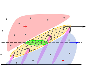
Figure 1. An illustration of the experimental set-up, showing the green laser illumination of the wall-parallel plane ( $x$–
$x$– $z$) near the bottom wall of the test section. Green and red dots represent the glass tracer particles and fluorescent inertial particles, respectively. Two cameras were positioned above and below the test section, each with colour filters to record the two types of particles simultaneously. The resulting filtered fields are illustrated above and below the test section, in place of the cameras.
Table 1. Parameters for the underlying boundary layer flow and the location of the laser sheet at wall normal height,  $h$. The boundary layer thickness, $\delta$, represents $\delta _{99}$. Mean flow profiles and streamwise energy spectra are provided in Appendix A.

The flow was seeded with small, glass tracers (Sigma-Aldrich 440345-500G,  $1.1\ {\rm g}\ {\rm ml}^{-1}$, diameter $9\unicode{x2013}13\ \mathrm{\mu}{\rm m}$) to measure the velocity field, and large polyethylene fluorescent particles (Cospheric UVPMS-BR-1.20 $75\unicode{x2013}90\ \mathrm {\mu }{\rm m}$, $1.2\ {\rm g}\ {\rm ml}^{-1}$, diameter $75\unicode{x2013}90\ \mathrm {\mu } {\rm m}$) to identify particle clustering. The volume fractions for the tracers and particles were $6.7 \times 10^{-5}$ and $9.2 \times 10^{-6}$, respectively.
The key parameter describing the relative inertia of the particles compared with that of the carrier flow, and thus the extent of coupling, is the Stokes number,  $St$, which is the ratio of the viscous time scale of the particle, $\tau _p$, to an appropriate time scale of the flow, $\tau _f$. The viscous time scale, in the limit of infinitesimal particle Reynolds number, ${Re}_p \equiv {d_p^3 \rho _f g (\rho _p-\rho _f)}/{18 \mu ^2} \ll 1$, is given in terms of the particle density, $\rho _p$, the fluid density, $\rho _f$, the particle diameter, $d_p$, and the dynamic viscosity, $\mu$, as $\tau _p= {(\rho _p-\rho _f)d_p^2}/{18\mu }$ (Eaton & Fessler Reference Eaton and Fessler1994). For heavy particles, $\rho _p \gg \rho _f$, this viscous time scale is approximately $\tau _p \approx {\rho _pd_p^2}/{18\mu }$ (Stokes Reference Stokes1851).
The flow time scale  $\tau _f$ for turbulent flows can be defined in terms of the Kolmogorov scales, as $\tau _\eta = (\nu /\epsilon )^{1/2}$ (via the dissipation rate, $\epsilon$, and kinematic viscosity, $\nu$) following Monchaux et al. (Reference Monchaux, Bourgoin and Cartellier2010) and Aliseda et al. (Reference Aliseda, Cartellier, Hainaux and Lasheras2002); or in terms of the friction velocity as $\tau _\nu = {\nu }/{u_\tau ^2}$, following Yamamoto et al. (Reference Yamamoto, Potthoff, Tanaka, Kajishima and Tsuji2001) and Zhao, Andersson & Gillissen (Reference Zhao, Andersson and Gillissen2013). The dissipation rate in the log layer was estimated from the planar PIV data, assuming that it is in balance with the production rate (see Brouwers (Reference Brouwers2007) for discussion). The production itself was approximated as $\mathcal {P} \approx -\overline {uv}({\partial U}/{\partial y}) -\overline {vv}({\partial V}/{\partial y})$, where the remaining contributions to the production are assumed negligible, following Blackman et al. (Reference Blackman, Perret, Calmet and Rivet2017), yielding a dissipation rate of $\epsilon \approx 0.6\ {\rm m}^2\ {\rm s}^{-3}$.
Table 2 summaries the Stokes numbers and mass/volume fractions for the particles used in this experiment, along with a selection of relevant past studies performed in a channel flow, boundary layer and in experiments with HIT. The current volume fraction for inertial particles was consistent with previous studies, although the mass fraction is much lower, due to the smaller density of the current particles. Nevertheless, the Stokes number of the inertial particles is nearly two orders of magnitude larger than the velocity tracers due to their size. According to Brandt & Coletti (Reference Brandt and Coletti2021), the low volume fraction in all of these experiments is indicative of the one-way coupling regime between the fluid and inertial particles, which is better suited to observe the influence of large-scale coherent motions of the canonical boundary layer on the particle clustering.
Table 2. Range of particle parameters for current experiment (top) and past clustering studies (bottom). The Kolmogorov time scale,  $\tau _\eta$, was calculated using the dissipation rate obtained via the balance of production and dissipation in the log layer. Here DNS is direct numerical simulation.

2.2. Particle and velocity field processing
The fluorescent, inertial particles had an excitation peak at 575 nm and an emission peak at 607 nm. Therefore, the fluorescent light of the particles was isolated from the laser light by using a notch filter (Chroma, ZET532nf) blocking the laser wavelength,  $527$ nm. The reflected light of the tracer particles was isolated from the fluorescent light by using a bandpass filter (Chroma, ET525/30m) overlapping the same wavelength. Because the fluorescent particles also reflected light at the laser wavelength, albeit at much weaker intensity than the glass tracers, the slight signature of the fluorescent particles was removed from the tracer image using a digital masking procedure, which also eliminated noise from the particle image. The fluorescent particles were masked using a fixed intensity threshold ( $1000$ out of $4096$ grey levels). The resulting binary mask was then used for measuring the particle clustering behaviour, described in § 3, as well as for masking out the low-intensity reflections of the fluorescent particles from the velocity tracer images, prior to PIV processing of the velocity field. The size distribution of the fluorescent signature of the particles is discussed in the next section, § 2.3.
The masking and PIV processing was performed using commercial software (Davis 10.1.1). Five independent recordings were performed at 800 Hz with  $\Delta t = 130\ \mathrm {\mu }{\rm s}$ ( $\Delta t^+= 1.1$) between image pairs. The duration of each recording was approximately 188 eddy turnover times ( $\delta / U_\infty$), yielding a total temporal record length of around 940 eddy turnover times. The convergence of all statistical quantities was verified by random sampling of the snapshots across different eddy turnover times. Perspective correction was applied to the image pairs according to a planar calibration image, and a sliding-average background of size 8 pixels was subtracted. The multipass vector calculation included an initial pass of a square $32\times 32$ pixel window, followed by a second pass with a $16\times 16$ pixel circular window. To avoid spatial aliasing, interrogation windows with $50\,\%$ overlap were applied for both passes. The correlation value was also calculated for the PIV algorithm and vectors with a correlation value lower than 0.5 were deleted. Vectors with greater deviation than two times the standard deviation were removed and replaced with interpolated velocity data. The spatial resolution of the underlying images was $0.054\ {\rm mm}\ {\rm pixel}^{-1}$, resulting in a spatial resolution of the velocity field, after PIV processing, of $\Delta x^+ = 39.5$. The spatial resolution for the particle field was $\Delta x^+ = 4.9$.
The particle velocities themselves were obtained by PTV applied to the pre-binarized fluorescent particle image pairs, where the time delay between pairs was  $130\ \mathrm {\mu }{\rm s}$. A ‘Laplace of Gaussian’ filter was applied to the particle images first, and the particle centres were obtained with subpixel accuracy after a Gaussian interpolation, following Heyman (Reference Heyman2019). The velocities of the particles were then calculated by matching particle pairs between two pulses, using the numerical approach described in Janke, Schwarze & Bauer (Reference Janke, Schwarze and Bauer2020). More than $95\,\%$ of particles in the two pulses were matched with high confidence; the remaining $5\,\%$ particle losses were due to out-of-plane particle motions.
2.3. Particle cross-section homogenization
The threshold binarization of the fluorescent particle field had the effect of exaggerating the size of some particles due to their greater scattering cross-section. The variations in scattering cross-section can result from both variations in the physical size of the particle (which, in this case is relatively small for highly monodisperse particles) and variations in the intensity of incident light, which varies with the location of the particles relative to the peak intensity of the laser sheet as noted by Raffel et al. (Reference Raffel, Willert, Scarano, Kähler, Wereley and Kompenhans2018). In order to identify particle clusters purely by their spatial distribution, without bias due to the scattering cross-section of individual particles, the binarized particle images were homogenized to generate a field in which all particles were represented with a uniform number of pixels (i.e. perfectly monodisperse).
The homogenization process first eliminated all binary pixel clusters with fewer than two pixels. The pixel clusters were then fitted by an ellipse where the major ( $d_{maj}$) and minor ( $d_{min}$) axes of the ellipse were defined by the second moments of the underlying cluster area, as described in Appendix A of Haralock & Shapiro (Reference Haralock and Shapiro1991). The image processing was performed using MATLAB. Prior to homogenization, the mode of the major axes was approximately $3.7$ pixels, and the distribution was clearly not singular, as desired. Thus, all of the irregular shaped (polydisperse) pixel clusters were replaced by square clusters at their original centroid locations with side length 3 pixels, corresponding to a major axis of approximately $3.5$, in order for the homogenized particle field to retain particles of similar size as in the original particle field, but perfectly homogeneous in shape and pixel count.
3. Cluster identification
The homogenized binary particle field was used to detect spatially significant clusters of particles using two different techniques: Voronoi tessellation and spatial wavelet identification.
3.1. Voronoi tessellation
The Voronoi technique was implemented following the approach of Monchaux et al. (Reference Monchaux, Bourgoin and Cartellier2010) and Monchaux et al. (Reference Monchaux, Bourgoin and Cartellier2012). We first analysed each homogenized particle field to obtain the unique Voronoi tessellation of cells describing that field, as shown in figure 2(a). Each cell represents the region of the field closer to the particle it encloses than to any other particle. A cluster of particles is defined as a region of contiguous cells, each of area  $A$, where the area of each cell normalized by the average area of all cells, $\langle A \rangle$, $\bar {A} = A/\langle A \rangle$, is smaller than some normalized threshold area, $\bar {A}_c$, that would be expected were the particles distributed spatially by a uniform random distribution with the total number of particles specified by a Poisson point process, with expected value, $\lambda$, set equal to the average number of particles per field detected in the real experiments. (An alternative method for generating synthetic particle fields with fixed numbers of particles per field will be described in § 3.2.2.)

Figure 2. (a) A sample particle field with particles denoted by blue points surrounded by the black edges of the Voronoi cells. Cells with area  $\bar {A} < \bar {A}_c$ are shaded grey. (b) Probability density ( $p)$ of normalized Voronoi cell areas ( $\bar {A}$) for: $10^5$ synthetic fields generated by a Poisson process (dashed, red) with shape parameter equal to the mean number of particles in the experimental particle fields; and $4425$ experimental particles fields (solid, black). The vertical dashed (black) line represents the crossing point between the two p.d.f.s ( $\bar {A}_c= 0.68$) which distinguishes between clustered and non-clustered cells.
Figure 2(b) shows the distribution of the cell areas from the synthetic Poisson fields (dashed) and measured particle fields (solid). Cells bordering the edge of the measurement region were eliminated. The intersection point between the two distributions is used as the threshold area value,  $\bar {A}_c$. Cells with area smaller than this threshold represent regions of unusually dense particle concentration and are marked grey in figure 2(a).
The contiguous regions of grey cells in figure 2(a) were treated as particle clusters. Note that here, contiguity includes cells that share a common edge and even cells connected by only a single vertex. To quantify the size and orientation of these very irregular clusters of cells, each cell cluster was fitted to an ellipse by least squares (following the same procedure described in § 2.3 for the pixel clusters) and the major and minor axes, denoted  $L_{maj}$ and $L_{min}$, respectively, and the orientation angle, $\theta$, measured with respect to the streamwise direction, were extracted. The characteristic ellipses associated with the Voronoi clusters are illustrated in figure 3(a). This ellipse fitting was done for consistency with the wavelet analysis presented below in § 3.2, in which the wavelets are naturally characterized by the geometric parameters of an ellipse. But the characteristic scale of the Voronoi clusters can also be calculated directly by their total area and perimeter, as done by Monchaux et al. (Reference Monchaux, Bourgoin and Cartellier2010).

Figure 3. (a) Ellipses identifying the cell clusters previously identified in the example particle field from figure 2(a), marked with red solid lines. (b) Joint p.d.f. ( $p$) of the major and minor axis lengths of ellipses bounding the Voronoi clusters, including all orientation angles. The domain of the map represents the physical measurement limits of the present experiment, including the definitional requirement for all ellipses that $L_{maj} > L_{min}$.
The parameters describing the cluster ellipses provide a convenient statistical perspective on both the size and orientation of particle clusters in the flow. Figure 3(b) shows the joint p.d.f. of the cluster major axes,  $L_{maj}$, with respect to the minor axes, $L_{min}$, averaged over all orientation angles. The vast majority of particle clusters detected by the Voronoi technique is smaller than $\delta$ and there are almost no large clusters detected with a size of $2\delta$ or greater. The most probable clusters are slightly anisotropic, with $(L_{maj}/\delta,L_{min}/\delta ) \approx (0.29,0.18)$. In terms of the actual area of the Voronoi cluster, the mode was approximately $\sqrt {A_v}/\delta \approx 0.2$. These clusters are a bit larger than the typical size detected in previous studies; for instance, Zhu et al. (Reference Zhu, Pan, Wang, Liang, Ji and Wang2021) reported the most probable Voronoi area as $\sqrt {A_v}/\delta \approx 0.04$. The difference is due to the particle volume fraction: in Zhu et al. (Reference Zhu, Pan, Wang, Liang, Ji and Wang2021), the volume fractions are $7 \times 10^{-5}$ and $11\times 10^{-5}$, approximately one order of magnitude higher than the volume fraction in present experiment, $9.2 \times 10^{-6}$.
The tendency of the Voronoi approach to detect small-scale features is also apparent in reports of clustering in HIT by Monchaux et al. (Reference Monchaux, Bourgoin and Cartellier2010). There, they reported an inverse power law distribution (with an exponent of  $-2$) of particle cluster areas, without any particular characteristic length scale, and all of the clusters identified were nearly an order of magnitude smaller than the integral length scale of the flow (granting that their field of view in the streamwise direction extended only approximately two integral length scales). Using a box-counting technique, Aliseda et al. (Reference Aliseda, Cartellier, Hainaux and Lasheras2002) were able to obtain a typical cluster size for HIT of approximately 10 Kolmogorov length scales, again about an order of magnitude smaller than the integral scales of their flow.
Based on Voronoi analysis alone, we might conclude that the significant organization of particles is confined to the small scales and does not extend in space as far as the coherent momentum structures, associated with LSMs. However, the Voronoi analysis is inherently limited in its ability to detect such extended features, because even a single non-contiguous cell can interrupt a cluster. In other words, multiple contiguous cells are needed to instantiate a large-scale cluster, but only a single large cell can prevent one from being detected, and thus we expect a bias towards the detection of small-scale features. In particular, if large-scale features are the result of a superposition of small-scale features, as is hypothesized in the case of momentum structures, then any separation between the constituent small-scale features will prevent detection of the resultant large scales by the Voronoi technique. We therefore turn to an alternative technique for spatial cluster identification in order to identify large-scale particle clustering behaviour without this bias: the wavelet.
3.2. Wavelet transformation
In order to identify large-scale particle clusters, the homogenized binary particle map was transformed via a wavelet transform. The wavelet transform represents a convolution of a wavelet kernal,  $\psi (x,z)$, with the underlying wall-parallel ( $x$–
$x$– $z$) particle field in order to detect clusters of particles that correspond to the wavelet geometry. Farge (Reference Farge1992) noted that the continuous wavelet transform is better suited for tracking coherent structures, although worse for efficient modal representation of data. Because of this, the astrophysics studies referenced in § 1.3 generally employed the continuous wavelet transform to identify galaxy clusters, whereas previous turbulence studies utilized the discrete transform to produce efficient, low-order representations of turbulent flow fields.
3.2.1. Anisotropic wavelets
The wavelet employed for the cluster detection was the anisotropic (real-valued) Mexican hat wavelet as defined in Antoine et al. (Reference Antoine, Murenzi, Vandergheynst and Ali2004), which allows for independent variations in the minor axis length of the wavelet,  $L_{min}$, the aspect ratio of the major and minor axes, $\varepsilon = L_{max}/L_{min}$, and the major axis orientation angle $\theta$, and is particularly well suited for feature detection applications, as noted by Hou & Qin (Reference Hou and Qin2012). The wavelet parameters are illustrated in figure 4(a). The major and minor axes describe the spatial domain of an ellipse that coincides with the positive annulus of the wavelet. (Note that not all anisotropic Mexican hat wavelet definitions are the same – see the discussion in Appendix B for details.)

Figure 4. (a) A representative wavelet amplitude map, illustrating the signed magnitude of the wavelet (red for the positive annulus, blue for the negative), showing its major and minor axes,  $L_{maj}$ and $L_{min}$, and its orientation angle, $\theta$. The inset illustrates the cross-sectional slice of the wavelet across its major axis, showing the magnitudes of the positive (red) and negative (blue) annuli. (b) A grid of the wavelet dimensions and aspect ratios, where each intersection indicates a particular combination of wavelet parameters. The dashed horizontal line indicates the streamwise domain size.
As the Mexican hat wavelet is convolved with a particle field, the resulting wavelet coefficient field represents the magnitude of the spatial particle clustering within the positive annulus of the wavelet, discounting those particles that appear in the negative annulus, and ignoring particles situated beyond that region. Therefore, the spatial parameters which define the positive annulus of the wavelet also characterize the geometric clustering of the particles detected by that wavelet. The axes are thus conceptually analogous to the elliptical axes that were used to bound the grey cells of the Voronoi clusters in the previous section. By varying the wavelet parameters,  $(L_{min},\varepsilon,\theta )$, different shapes and orientations of particle clusters were detected.
The wavelet transform was calculated over 10 linearly spaced minor axis scales,  $L_{min}$, starting from the smallest scale of interest, $0.1 \delta$ or $215 \nu /u_\tau$, chosen to comfortably exceed the typical spanwise length scale of the near wall streaks (see Smith & Metzler Reference Smith and Metzler1983), and extending to $0.73 \delta$. This resulted in the largest major axis within the measurement domain, $L_{maj} \approx 5.9$, obtained when the minor axis is multiplied by the largest aspect ratio considered. The aspect ratios were linearly spaced between $\varepsilon = 1$ and $10$. The resulting set of wavelet dimensions is illustrated in the map in figure 4(b). Every combination of wavelet dimensions was deployed at all orientation angles, $\theta = 0^\circ, 15^\circ, 30^\circ,\ldots, 180^\circ$, resulting in a total number, $n$, of unique wavelets, $(L_{min},\varepsilon,\theta )_j$.
Each particle field,  $i = 1,\ldots,N$, was transformed into the wavelet domain for each unique wavelet, $j = 1,\ldots,n$, yielding maps of wavelet coefficients $C_{ij}(x,z)$. The continuous wavelet was implemented via a Fourier transform technique (‘cwtft2’ in MATLAB), where finite boundary effects were avoided by assuming a periodic particle domain.
Following the approach of Escalera & Mazure (Reference Escalera and Mazure1992), the locations,  $(x^*,z^*)_{ij}$, of the relative maxima, $C^*_{ij}(x^*,z^*)$, of the wavelet transform field were identified using a sparse peak finder. These maxima represent strong regions of local particle clustering at the scale (and orientation) of a specific wavelet. However, the presence of a relative maximum alone does not necessarily indicate a statistically significant spatial density of particles. In order to ascertain whether the maximum is significant, it was compared with a threshold value of the wavelet coefficient maximum, $\hat {C}_{95}$, at the 95th percentile level, determined via the wavelet transform of a uniform, spatial, random process with the same number of particles as the field of interest. To accomplish this comparison, synthetic particle fields were generated with a uniform random process in order to establish the statistical threshold of significance.
3.2.2. Significance testing via synthetic particle fields
The threshold for significant wavelet maxima,  $\hat {C}_{95}$, was determined as a function of the wavelet geometric properties $L_{min}$ and $\varepsilon$ (excluding $\theta$ by symmetry arguments). However, the wavelet coefficient field was also found to depend on the size of the particles used in the homogenization procedure, $d_h$ (measured in pixels), as well as the number density of particles in a particular field, $\phi _p$, where number density is defined as the number of particles per field area.
The particle number density dependence also influenced the Voronoi technique described above, and was taken into account via the generation of synthetic particle fields. There, the random fields were based on a Poisson point process, in which the number of particles per field was selected from a Poisson distribution with the same mean number of particles as the measured fields. In this way, the dependence on number density was swept into the threshold generation implicitly. An alternative approach, adopted in the wavelet studies of Slezak et al. (Reference Slezak, Bijaoui and Mars1990) and Escalera & Mazure (Reference Escalera and Mazure1992), involved generating random fields with a fixed number of particles, identical to the experimental field of interest. In this way, the confounding effect of number density was eliminated from the threshold completely, not just in an average sense. The difficulty with using a fixed number of particles is that every new experimental particle field would require a corresponding set of synthetic fields with that same particle density to generate a new statistical threshold. Therefore, in this study, we chose the middle ground between these approaches: explicitly modelling the wavelet field dependence on the number density,  $\phi _p$, to obtain higher accuracy than the Poisson assumption (which had previously been criticized by Escalera et al. (Reference Escalera, Slezak and Mazure1992)) without the computational cost of calculating separate synthetic fields for each new measured field.
The threshold wavelet maximum,  $\hat {C}_{95}(L_{min},\varepsilon,d_h,\phi _c)$, was determined by (1) generating large sets of random particle fields for each parameter value; (2) finding the converged distribution of wavelet maxima $C^*$ for each set; (3) selecting the 95th percentile value of $C^*$ to define the threshold, $\hat {C}_{95}$, for each particular wavelet; and (4) fitting an empirical function to describe parametric dependence of $\hat {C}_{95}$ on these individual wavelet parameters. The functional representation of the threshold reduced the computational burden of calculating new synthetic fields for every possible combination of wavelet parameters. To obtain a statistically converged threshold, each set of wavelet parameters required a large number of synthetic fields (resulting in more than $2.5 \times 10^6$ maxima detected per wavelet). The convergence behaviour and accuracy of the threshold, $\hat {C}_{95}$, is discussed in Appendix C.
Figure 5 shows the variation of the threshold,  $\hat {C}_{95}$, as a function of the particle size, $d_h$ in pixels (figure 5a), the particle number density (per frame), $\phi _p$ (figure 5b), the wavelet minor axis, $L_{min}$ (figure 5c), and the aspect ratio, $\varepsilon$ (figure 5d). These different relations were collapsed into the approximate threshold function,
 \begin{align} \hat{C}_{95}(d_h,L_{min},\varepsilon,\phi_p) = \hat{C}_{95,0} \left(\frac{d_h}{d_{h,0}}\right)^{\alpha_d} \left(\frac{\phi_p}{\phi_{p,0}}\right)^{\alpha_\phi} \left(\frac{L_{min}}{L_{{min},0}}\right)^{-\alpha_L\left({\phi_p}/{\phi_{p,0}}\right)^{\beta_L}} \!\!\left(\frac{\varepsilon}{\varepsilon_0}\right)^{-\alpha_\varepsilon \left({\phi_p}/{\phi_{p,0}}\right)^{\beta_\varepsilon}}, \end{align}
where each parameter,  $A$, is normalized by a characteristic value, $A_0$, and then raised to a power that itself can depend on number density, in the form: $\alpha _A \phi _p^{\beta _A}$. The fit was performed by nonlinear least square regression, and the range of parameters and their resulting exponents and corresponding standard errors, are listed in table 3. The quality of the fit was assessed by comparing the actual statistical percentile of the synthetic data corresponding with the model threshold (i.e. the effective threshold percentile) versus the design percentile of $95$ from which the model was formulated. It was found that more than $87\,\%$ of the effective threshold percentiles were within the percentile of $95\pm 2.5$, such that using the model threshold was likely to produce nearly the same effective significance level as direct examination of the distribution of maxima from synthetic fields.

Figure 5. The variation of  $\hat {C}_{95}$ with respect to (a) homogeneous particle size, $d_h$, holding the other parameters fixed; (b) particle number density, $\phi _p$; (c) wavelet size, $L_{min}$; (d) wavelet aspect ratio, $\varepsilon$. The individual points (red circles) are chosen from within the range given in the second column of table 3. The solid lines are fitted power laws with exponents given in the last two columns of table 3.
Table 3. Nonlinear, least-squares, best-fit parameters for the wavelet maxima threshold model described in (3.1). The uncertainty is listed as standard error, where  $n=132$ unique wavelets were used for fitting the power-law surface.

The threshold relation in (3.1) was applied to the experimental particle fields to determine which wavelet maxima represented statistically significant spatial particle clusters. Unlike the threshold used previously in the Voronoi analysis, the percentile-based approach adopted here allows for the choice of significance level, and provides for an intuitive interpretation of the particle clusters. Significant particle clusters are defined in terms of the likelihood of those clusters appearing in a field of randomly distributed particles. Clusters of particles that result in a wavelet maximum in the top 5 % of all wavelet maxima from randomly distributed particle fields are defined as statistically significant. Other threshold values, from 10 % to 1 %, were also examined and result in similar trends as presented below, with some slight variation in the prominence of less likely (i.e. more extreme) cluster sizes.
3.2.3. Wavelet-identified clusters
Figure 6(a) illustrates the same example particle field used above for the Voronoi analysis, with all the significant wavelet maxima circumscribed by their corresponding positive annulus ellipses, showing the regions of significant, coherent clustering. The wavelet ellipses in the example appear to encompass all of the particles previously identified by the Voronoi analysis, along with a substantial number of additional particles not identified by the Voronoi. Over all the particle fields,  $94\,\%$ of the particles associated with Voronoi clusters were also associated with wavelet clusters. And while the Voronoi analysis placed approximately $32\,\%$ of all particles inside clusters, the wavelet analysis placed nearly $72\,\%$ of all particles inside clusters. Of course, this number could be reduced by increasing the statistical significance threshold. But more important than the difference between these techniques in the number of particles identified within clusters is the difference in appearance of the cluster-bounding ellipses. Unlike the Voronoi ellipses, the wavelet ellipses overlap each other, i.e. multiple different wavelets detect the same underlying clusters of particles, but at different scales.

Figure 6. (a) Ellipses identifying the wavelet clusters, marked with red solid lines, overlayed on the Voronoi clusters from figure 3(a). (b) Joint p.d.f. of the two ellipse axes of the wavelet clusters for all orientation angles.
The overlapping of ellipses is indicative of the hierarchical nature of the wavelet detection technique, which identifies small clusters whose superposition creates the appearance of larger clusters, and also those large clusters themselves. This overlap reveals a hierarchy of particle clustering, similar to the momentum hierarchies familiar from wall-bounded turbulence. However, this redundancy also creates an interpretative difficulty, because the distribution of wavelet clusters inherently conveys a cumulative picture, potentially double-counting ‘child’ clusters within ‘parent’ clusters. Thus special care is required when analysing the distribution of the geometric cluster parameters obtained by the wavelet technique.
Figure 6(b) shows the joint p.d.f. of the cluster major axes,  $L_{maj}$, with respect to the minor axes, $L_{min}$, averaged over all orientation angles, comparable to the joint p.d.f. of the Voronoi ellipses shown earlier in figure 3(b). The Voronoi ellipse parameters were continuously distributed and thus the joint p.d.f. could be constructed by a standard histogram technique. However, the wavelet ellipse parameters constitute a finite set of discrete values, illustrated by the grid in figure 4(b), and thus linear interpolation was used to obtain a continuous probability density surface, i.e. filling in between the grid locations. The outer boundary of the grid is shown in solid black outline. The final Voronoi and wavelet p.d.f.s were linearly interpolated to the same, underlying grid density for comparison.
The wavelet cluster joint p.d.f. shows a high concentration of isotropic clusters, ranging from the smallest wavelets up to the largest (along the bottom edge of the graph), with the highest probability clusters being small, nearly isotropic clusters consistent with the Voronoi distribution. However, unlike the Voronoi distribution, the wavelet p.d.f. also shows a substantial number of large-scale clusters with major axis larger than  $1 \delta$ in length, including both highly anisotropic clusters as well as nearly isotropic clusters. These large scales are consistent with the overlapping, large-ellipses noted above, and thus are assumed to be associated with the hierarchical superposition of smaller particle clusters.
4. Particle clusters and hierarchies
To better understand the content of the large-scale clusters identified by the wavelet technique, we first compare the joint p.d.f.s of the wavelet and Voronoi clusters in figure 7(a), superimposing the contour lines from the Voronoi joint p.d.f. in figure 3(b) over the colour levels of the wavelet joint p.d.f. from figure 6(b).

Figure 7. (a) Joint p.d.f. for the characteristic cluster ellipses for the wavelet technique (colour levels) and the Voronoi technique (contour lines, black) for all orientation angles; the probability peak for Voronoi clusters and wavelet clusters are marked by magenta square and diamond, respectively. (b) The conditional joint p.d.f. of the wavelet technique for all clusters whose centroid falls within the large-scale cluster corresponding to the label (b) in panel (a) of the figure. (c) The conditional joint p.d.f. of the wavelet technique for all clusters whose centroid falls within the large-scale cluster corresponding to the label (c) in panel (a) of the figure.
As noted above, the major axes of most Voronoi clusters are smaller than  $\delta$, with almost no clusters greater than $\delta$, while we can detect a significant amount of clusters that are greater than $\delta$ in the wavelet analysis. However, the peak of the Voronoi cluster distribution, $(L_{maj}/\delta, L_{min}/\delta ) = (0.29, 0.18)$, is actually slightly greater than the wavelet peak location, $(L_{maj}/\delta, L_{min}/\delta ) = (0.1, 0.1)$, which corresponds to the smallest wavelet, i.e. the basic building block for superposition of particle clusters. The Voronoi and wavelet peaks are marked by the magenta square and diamond symbols, respectively, in figure 7(a). This is likely due to the hierarchical nature of the wavelet identification: all wavelet clusters can, in principle, be decomposed into smaller clusters, down to the smallest measurable wavelet scale, whereas a Voronoi cluster represents only a single scale and does not allow for the possibility that the cluster is actually composed of sub-clusters, i.e. ‘children’. So, the Voronoi analysis is actually biased against the smallest possible constituent clusters and thus displays a slightly larger peak cluster size than the wavelet.
Besides the peak for small clusters, the wavelet distribution also shows peaks at the large scales which are not apparent in the Voronoi analysis, exemplified by the points labelled (b) and (c) in figure 7(a). Point (b) represents strongly anisotropic, large-scale clusters of size  $(L_{min}/\delta,L_{maj}/\delta ) = (0.24, 1.92)$ which are similar to the dimensions of LSMs in turbulent wall-bounded flows. Point (c) represents mildly anisotropic, large-scale clusters of size $(L_{min}/\delta,L_{maj}/\delta ) = (0.66, 1.98)$. Because we expect these large-scale peaks in the cluster distribution to represent a superposition of smaller scale clusters, we reconstruct a conditional version of the joint p.d.f., including only clusters whose characteristic ellipses overlap the ellipses of the points (b) and (c). These conditional joint p.d.f.s are displayed in figure 7(b,c).
The conditional p.d.f. of cluster size in figure 7(b) shows that the large-scale, highly anisotropic (long, thin) clusters detected by the wavelets are predominantly coincident with very small, isotropic clusters (along with a small number of large-scale, isotropic clusters). In other words, long, thin particle clusters at the scale of the LSMs can be thought of as a superposition of small-scale isotropic clusters, reminiscent of the superposition explanation of large-scale, long meandering momentum streaks suggested by Adrian et al. (Reference Adrian, Meinhart and Tomkins2000), among others. Similarly, the conditional p.d.f. of cluster size in figure 7(c) shows that the large-scale, nearly isotropic clusters detected by the wavelets are predominantly coincident with the long, thin clusters at point (b), in addition to the small-scale isotropic clusters, which again substantiates the idea that the wavelets detect a wide range of ‘parent’ clusters which are constituted of one or more generations of smaller ‘child’ clusters.
Unfortunately, while the wavelet technique is adept at determining the hierarchical relationships between parent and child clusters, there is no objective way to assign the hierarchy of related particles a unique, characteristic scale. In other words, there is no direct comparison with the unique clusters identified by the Voronoi analysis. However, recent work on data-driven wavelet selection by Floryan & Graham (Reference Floryan and Graham2021) may provide a unique wavelet decomposition useful for making such characterizations in the future.
The identification of spatial particle clusters from instantaneous measurements, either via the Voronoi or wavelet techniques, leaves open the question of the dynamical significance of the detected clusters: do the instantaneous clusters exhibit an influence on the velocity of the particles included within them? And if so, how do the particle velocities vary, on average, with the size of their corresponding clusters?
5. Particle velocities within clusters
5.1. Particle velocity distribution
To study the velocity of the particles within the clusters, we first present the overall probability distribution of the fluid velocity,  $u$, and the particle velocity, $u_p$, irrespective of the clusters, in figure 8(a). The fluid velocity distribution (in blue) is bimodal reflecting the signature of the high and low speed streaks in the wall-parallel plane at the height of the log layer. The particle velocity distribution is unimodal with negative skew, where most particles are measured as travelling faster than the mean velocity. In fact, the mode of the particle velocity distribution coincided roughly with the velocity of the near-wall, high-speed streaks, although the particle velocities are broadly distributed.

Figure 8. (a) Distribution of overall fluid velocity,  $u$ (blue) and particle velocities, $u_p$ (red). (b) Distribution of particle velocities in-clusters (solid) and out-of-clusters (dashed) for the Voronoi method. (c) In-cluster and out-of-cluster particle velocities for the wavelet method.
In the hairpin paradigm, Tomkins & Adrian (Reference Tomkins and Adrian2003) argued that the high-speed streaks are associated with the forward flow induction produced by aligned hairpin legs. Dennis & Nickels (Reference Dennis and Nickels2011) provided additional experimental evidence in support of this view, via conditional averaging, showing that the high-speed regions appear adjacent to the hairpin legs, due to the forward flow induction. However, this does not necessarily mean that the particles are dynamically associated with the high-speed streaks themselves. They could just as easily be associated with the sweeping events induced along the backbone of the hairpin packet, as argued by Zhu et al. (Reference Zhu, Pan, Wang, Liang, Ji and Wang2021), and still obtain a similar velocity distribution due to the same induction process.
The overall particle velocity distribution was then conditioned on whether the particles in question were part of a cluster or not. For the Voronoi technique, shown in figure 8(b), the difference between the in-cluster and out-of-cluster particle velocity distributions was very subtle, with in-cluster particles exhibiting a slightly higher average velocity. For the wavelet technique, shown in figure 8(c), the difference was a bit more pronounced, again with in-cluster particles travelling faster. In both cases, the differences were not significant enough to drawn any inference about the relative position of the in-cluster particles with respect to coherent motions in the momentum field.
5.2. Particle clusters convection scaling
In order to establish the physical orientation of the particle clusters in the turbulent boundary layer with respect to the coherent structures, conditional averaging of the momentum field was attempted. However, as Zhu et al. (Reference Zhu, Pan, Wang, Liang, Ji and Wang2021) previously reported, such averaging is impractical when dealing with very low particle concentrations in the flow. Therefore, they employed other inferential techniques, including quadrant analysis in the vicinity of particles, as well as conditional spectral techniques, in order to argue that particles tended to collect along the sweep and ejection events that demarcate the outer envelope of hairpin packets (or, equivalently, uniform momentum zones). Here, we take a different approach towards inferring the particle orientation by exploiting the trend of particle velocities with respect to their cluster size. The convection velocity of coherent structures varies with their size, as has been known since the early work of Wills (Reference Wills1964), and thus so too should the velocity of particle clusters being convected by those structures.
In order to establish a relationship between cluster size and particle convection velocity, ideally we seek a unique convection velocity for each cluster size, ignoring the superposition effect. Thus, in this section, we focus on only the unique clusters identified by the Voronoi analysis. Then, to obtain the relationship between the particle velocities and the large-scale clustering, we averaged the particle velocities conditioned on the size of their associated Voronoi clusters in order to construct a map of the average particle velocities as a function of the cluster axis lengths. However, because the variation in particle velocities across different clusters was high, the averaging was performed using the ‘objective mapping interpolation’ technique, as described by McIntosh (Reference McIntosh1990), to obtain a smooth representation of the particle velocity trends. The maps of average particle velocities are shown in figure 9 for the Voronoi technique. Overlapping the particle velocities are the contour lines associated with the cluster size distribution from figure 3(b). A general trend of increasing particle velocity with cluster size is visible in both maps, with greater sensitivity to the variation in the ellipse minor axes compared with the major axes.

Figure 9. (a) Contour map of mean particle velocity for each Voronoi cluster as a function of  $L_{maj}$ and $L_{min}$ calculated via objective mapping interpolation. (b) Grey scatter points correspond to the mean particle velocity for each Voronoi cluster; the red line is a $0.06 \delta$-wide, rectangular moving-average of the scattered clusters; the black line is the average trend calculated from the contour map. The blue triangle represents the slope of coherent structure convection velocities, $u_c$, with respect to their streamwise wavelength, $\lambda _x$.
To observe the trends in more details, we plot the average variation in particle velocity with respect to the major and minor axes separately (averaging over the respective axes) in figure 9(b). These plots indicate the high variability in particle velocities per cluster by the cloud of grey points in the background (each point representing the average velocity of particles in a specific cluster), and then show the moving-average smoothing of the cluster velocities in red, and the average trends obtained by the ‘objective mapping interpolation’ technique in black. Both smoothing techniques resulted in a robust trend of increasing average particle velocity with cluster size.
Adrian et al. (Reference Adrian, Meinhart and Tomkins2000) provided a conceptual model for the convection velocity of different sized hairpin packets. Smaller packets exist closer to the wall and induce more intense backward velocity than larger packets, which reach farther from the wall, meaning that larger packets advect downstream faster. Del Alamo & Jimenez (Reference Del Alamo and Jimenez2009) quantified how the advection velocity of eddies increases with size as the attached eddies reach farther into the high-speed outer flow. They employed a ‘correlation height’ for the large-scale coherent structures and deduced the corresponding convection velocity from a convolution of the mean velocity profile of the flow in the vicinity of the correlation height.
The approximate convection velocity of different scale coherent motions was calculated following the approach of Del Alamo & Jimenez (Reference Del Alamo and Jimenez2009) and is shown in figure 10 as a function of streamwise and spanwise wavelengths of the motions, denoted  $\lambda _x$ and $\lambda _z$, respectively. The mean velocity profile used in the calculation was a channel flow reported by Hoyas & Jiménez (Reference Hoyas and Jiménez2008). The convection velocity averaged over spanwise wavelength is shown in figure 10(b), where the slope of the convection velocity with respect to the streamwise wavelength, $\lambda _x$ (for motions with $\lambda _x/\delta \gtrapprox 3.5$) is illustrated by a blue triangle. This slope triangle has also been inset in figure 9(b) for comparison with the slope of the particle advection velocity with respect to particle cluster size.

Figure 10. (a) Normalized convection velocity varying with streamwise ( $\lambda _x$) and spanwise wavelength ( $\lambda _z$) in the log layer. (b) The convection velocity profile averaged over $\lambda _z/\delta = 0\unicode{x2013}2$. The triangle displayed here and in figure 9(b) was calculated from the range of coherent motions $\lambda _x/\delta = 4\unicode{x2013}6$. Here $\delta$ corresponds to the half-channel height in the calculation of Del Alamo & Jimenez (Reference Del Alamo and Jimenez2009).
In figure 9(b), particle velocities and coherent motion convective velocities exhibit a similar trend, providing further evidence to support the notion that particle clusters collect on the back of coherent motions like hairpin packets, as proposed by Zhu et al. (Reference Zhu, Pan, Wang, Liang, Ji and Wang2021). However, in this slope comparison, the scale of the coherent motions was assumed much larger than that of the particle clusters. This discrepancy between the sizes of momentum and particle clusters may be the result of slicing the three-dimensional particle clusters in the wall-parallel measurement plane. The discrepancy might also be attributed to the hairpin thickness/height aspect ratio (see the attached eddy modelling of Perry & Chong (Reference Perry and Chong1982) and Marusic & Monty (Reference Marusic and Monty2019)) under the assumption that the particles are localized narrowly in the region of highest intensity straining flow adjacent to the vortex cores. Additional evidence that the particle clusters are associated with self-similar attached eddies can be found in the joint-distribution of the cluster shapes themselves, shown above in figure 3(b). Tracing along the peaks of the joint p.d.f. reveals that the most probable clusters have a roughly constant aspect ratio, independent of their size, which indicates wall-parallel slices through self-similar attached eddies that are involved in the transport of the particle clusters.
The particle cluster advection process, combining the previous report of Zhu et al. (Reference Zhu, Pan, Wang, Liang, Ji and Wang2021) with the convective velocity scaling of Del Alamo & Jimenez (Reference Del Alamo and Jimenez2009), and the current experiments, is illustrated schematically in figure 11. Figure 11(a) indicates the wall-parallel view of two particle clusters of different streamwise dimensions. Figure 11(b) shows the inference of the streamwise/wall-normal view of the particle clusters with respect to a hairpin packet. The particle clusters are shown in the yellow region indicating the outer interface of the hairpin packet which is illustrated as discrete, purple hairpins. The slice of the clusters in the measurement plane is shown in green. The sweep ( $Q4$) and ejection ( $Q2$) events are marked about the hairpin heads. Beneath the hairpin legs is a region of low-momentum fluid caused by the backward vortex induction described by Adrian et al. (Reference Adrian, Meinhart and Tomkins2000). Above the hairpin backbone is a region of higher momentum fluid being swept in towards the wall. The average particle velocity is denoted with a vector $\bar {u}_p$ exceeding that of the local mean flow in the measurement plane, $\bar {u}$, consistent with figure 9.

Figure 11. (a) Wall-parallel illustration of the particle field with two particle clusters labelled in green. (b) The streamwise/wall-normal inference of the particle clusters illustrated within the outer envelope of a hairpin packet (yellow), as proposed originally by Zhu et al. (Reference Zhu, Pan, Wang, Liang, Ji and Wang2021), but now taking into account the differential convection velocities of the particles due to two different size hairpin packets. The hairpins are illustrated in purple, the induced low-speed region beneath their legs in blue, and the high-speed fluid being swept in is shown in red. The vector,  $\bar {u}_p$ reflects the relative convection velocity of the particles and coherent structures compared with the mean flow, $\bar {u}$, as a function of the two hairpin packet sizes.
6. Conclusions
The large-scale clustering of inertial particles of modest Stokes number in a TBL was studied experimentally by two-colour, simultaneous PIV and PTV measurements in the wall-parallel plane of the log layer. Particle clusters were educed using two techniques: a standard Voronoi tessellation and a new implementation of the spatial wavelet transform. The wavelet approach was designed to detect the large-scale superposition of particle clusters that Voronoi tessellation misses by utilizing a wide range of wavelet scales and aspect ratios, up to the size of LSMs. The wavelet detection employed significance testing to determine statistically significant clusters based on the wavelet transformations of synthetic, random particle fields.
Both Voronoi and wavelet approaches identified the most common clusters at small-scales. For the Voronoi technique, the dominant cluster size was characterized by a bounding ellipse with major and minor axes:  $( L_{maj}/\delta, L_{min}/\delta )= (0.29, 0.18)$. For the wavelet technique the dominant cluster was a bit smaller, $( L_{maj}/\delta, L_{min}/\delta )= (0.1, 0.1)$. However, whereas the Voronoi technique detected very few clusters larger than the boundary layer thickness, the wavelet technique detected a significant number of clusters at the scale of the LSMs ( $2\unicode{x2013}3\delta$). These large-scale clusters were shown to be the result of superpositions of smaller scale clusters, by using conditional averaging of the cluster size p.d.f. In particular, the large-scale clusters were composed of long, thin (anisotropic) clusters, as well as very small, nearly isotropic clusters. The wavelet technique was thus found to successfully identify superpositions of particle clusters at a wide range of scales, including the scales of LSMs, but the Voronoi technique was better suited to identify unique clusters for the purpose of understanding cluster dynamics.
The dynamics of the clusters were studied indirectly by examining the velocities of the particles contained within them. The Voronoi detection technique, which identifies unique clusters, indicated an increase in the particle velocities as their corresponding cluster sizes increased, suggesting that the particles were being convected by coherent momentum structures moving faster than the local mean flow. The variation of convection velocity with cluster size was compared with the same variation reported for coherent momentum structures. Despite the noise in the data (due to local particle concentrations), the variations in convection velocity appeared consistent between particle clusters and coherent structures, adding support to previous reports that particle clusters tend to be advected on the backbones of hairpin packets.
Funding
This research was supported by grant no. 1704/17 from the Israel Science Foundation. The authors thank the anonymous referees for useful suggestions regarding the convergence verification.
Declaration of interests
The authors report no conflict of interest.
Appendix A. Streamwise/wall-normal statistics of the boundary layer
The mean velocity profile and premultiplied energy spectral density for the streamwise/wall-normal measurements of the flow without particles are shown in figure 12(a,b). The spatial resolution for the streamwise/wall-normal plane was  $0.056\ {\rm mm}\ {\rm pixel}^{-1}$, which means that for each velocity vector the spatial resolution was 41.2 wall units and 0.019 $\delta$ in outer units.

Figure 12. (a) The premultiplied, streamwise energy spectrum for the streamwise/wall-normal plane in the present study. Black crosses correspond to standard locations of the near wall cycle ( $y^+= 15$, $\lambda _x^+= 1000$) and outer peak ( $y/\delta \approx 0.06$, $\lambda _x/\delta = 6$). (b) Mean velocity profile (blue circles) and turbulence intensity profile (red triangles) for the present experiment at $Re_\theta = 5520$; black solid and dashed lines correspond to velocity and turbulence profiles from Fernholz & Finley (Reference Fernholz and Finley1996) ( $Re_\theta = 7140$). The grey rectangle represents the laser plane in the log layer ( $y= 2.5\unicode{x2013}3.3\ {\rm mm}$), with inner unit $y^+=229\unicode{x2013}302$.
Appendix B. Anisotropic Mexican hat properties
The anisotropic Mexican hat wavelet is written in different forms in a variety of texts and software packages, and therefore some care must be taken to avoid wavelets with side lobes in physical space, as is observed in the standard Mexican hat implementation, ‘mexh’ in MATLAB which is described in Misiti et al. (Reference Misiti, Misiti, Oppenheim and Poggi2013). The formula for ‘mexh’, in spectral space, can be obtained by the command ‘cwtftinfo2(‘mexh’)’, where the aspect ratio  $\varepsilon = (\sigma _x/\sigma _y)$ and the wavenumbers ( $\omega _x, \omega _y$) are non-dimensionalized by the scale of the wavelet, which is taken to be equal to $\sigma _y$. (Thus large aspect ratios refer to wavelets stretched in the $\hat {x}$-direction, and small aspect ratio refer to wavelets stretched in the $\hat {y}$-direction.) Fourier-transforming the spectral wavelet formula back to physical space yields
 \begin{equation} \psi_{mexh}(x,y) = \frac{2 {\rm \pi}}{\sigma_x \sigma_y^5} \left( \frac{x^2}{\sigma_x^4} + \frac{y^2}{\sigma_y^4} - \frac{\sigma_y^2}{\sigma_x^2} - 1 \right) \exp{\left[-\frac{1}{2 \sigma_y^2} \left(\frac{x^2}{\sigma_x^2} + \frac{y^2}{ \sigma_y^2} \right) \right]}. \end{equation}
However, the reference cited by the MATLAB documentation reports a different formulation in physical space, which does not correspond to the spatial transformation of their spectral definition. This physical space formulation is described by Antoine et al. (Reference Antoine, Murenzi, Vandergheynst and Ali2004) as
 \begin{equation} \psi(x,y) = \frac{1}{\sigma_x \sigma_y} \left( \frac{x^2}{\sigma_x^2} + \frac{y^2}{\sigma_y^2} - 2 \right) \exp{\left[-\frac{1}{2} \left(\frac{x^2}{\sigma_x^2} + \frac{y^2}{ \sigma_y^2} \right) \right]}, \end{equation}
and also matches (to within a prefactor of  $2 {\rm \pi}$) the form reported more generally in the research literature, e.g. Freeman et al. (Reference Freeman, Kashyap, Rosner and Lamb2002). The MATLAB formulation produces a wavelet with two discrete side lobes, whose contour levels do not form ellipses, and thus behaves significantly differently from the standard, anisotropic Mexican hat wavelets, as shown in figure 13.

Figure 13. (a) The non-normalized ‘mexh’ wavelet with  $\sigma _x = 3$ and $\sigma _y = 1$ as described in (B1). The dashed line represents the bound of the negative (blue) tails, which form two distinct lobes about the positive (red) core. (b) The non-normalized ‘gabmexh’ wavelet with the same scaling, absent any lobe structure, as described in (B3), which is used throughout the study.
However, MATLAB offers a second anisotropic implementation of the Mexican hat wavelet under the name ‘gabmexh’, which has the following formulation in physical space:
 \begin{equation} \psi_{gabmexh}(x,y) = \left( \frac{x^2}{\sigma_x^2} + \frac{y^2}{\sigma_y^2} - 2 \right) \exp{\left[-\frac{1}{2} \left(\frac{x^2}{\sigma_x^2} + \frac{y^2}{ \sigma_y^2} \right) \right]} \end{equation}
and this reproduces the elliptical, anisotropic Mexican hat wavelet generally seen in the literature, (B2), to within a scaling factor, which is compensated for by the appropriate normalization. Thus we adopt the ‘gabmexh’ throughout this study, with a  $\sigma _x \sigma _y$ normalization factor, to match the general anisotropic wavelet literature and to avoid the side lobes.
In order to include the orientation angle,  $\theta$, in the definition of the wavelet (B3), the unrotated $x'$–
$x'$– $y'$ coordinates should be transformed to $x$–
$x$– $y$ coordinates which are rotated by angle $\theta$ using the two-dimensional rotation matrix.
Appendix C. Wavelet threshold model properties
The shape of the p.d.f. of the extrema coefficients,  $C^*$, from the continuous wavelet transform of synthetic particle fields varies for different combinations of wavelet parameters and coverage ratios. For small wavelets relative to the features of the binary field at low coverage ratios, the p.d.f. is discontinuous, with a left-hand side that appears normal, representing partial overlap of the wavelets, rising to a maximum for perfect overlap, and then on the right-hand side a nearly uniform distribution of low probability representing overlap of multiple features within individual wavelets. As the wavelets become larger and the coverage ratio increases, the p.d.f. becomes bimodal and then eventually appears to converge to a beta distribution. Because the shape of the p.d.f. varies across wavelets, we employ an empirical percentile measure to determine the probability thresholds instead of trying to fit the shape of the p.d.f. to one of the canonical distributions. This empirical percentile technique works so long as the p.d.f. is sufficiently converged at the percentile of interest. More than $2.5 \times 10^{6}$ extrema for all cases were used to calculate the histogram and verify its convergence.
Figure 14 displays the true (empirical) percentile values corresponding to the  $\hat {C}_{95}$ values produced by (3.1). For a perfect model, the cumulative probability distribution function would appear as a step function at $0.95$. In reality, $96.2\,\%$ of the empirical percentiles are higher than $0.9$, i.e. the vast majority of empirical percentiles are within $\pm 5\,\%$ of the model assumption, indicating that the power-law model does a reasonable job of replicating the empirical percentile values.

Figure 14. Cumulative probability distribution function (CDF) of the true, empirical percentile values,  $Q$, corresponding to the $\hat {C}_{95}$ values produced by (3.1).


 Open access