


1 Introduction
Droplet dissolution dynamics is essential to many natural and industrial processes, such as coating, self-cleaning, surface spraying, etc. (Cazabat & Guena Reference Cazabat and Guena2010; Bhushan & Jung Reference Bhushan and Jung2011; Lohse & Zhang Reference Lohse and Zhang2015). It is also relevant to the extraction process used in drug delivery (Chou et al. Reference Chou, Lee, Yang, Huang and Lin2015). Droplet dissolution is in many ways similar to droplet evaporation, which has been studied extensively over the past decades (Picknett & Bexon Reference Picknett and Bexon1977; Deegan et al. Reference Deegan, Bakajin, Dupont, Huber, Nagel and Witten1997; Popov Reference Popov2005; Shahidzadeh-Bonn et al. Reference Shahidzadeh-Bonn, Rafai, Azouni and Bonn2006; Cazabat & Guena Reference Cazabat and Guena2010; Gelderblom et al. Reference Gelderblom, Marin, Nair, Van Houselt, Lefferts, Snoeijer and Lohse2011; Erbil Reference Erbil2012; Stauber et al. Reference Stauber, Wilson, Duffy and Sefiane2015; Hatte et al. Reference Hatte, Pandey, Pandey, Chakraborty and Basu2019; Pandey et al. Reference Pandey, Hatte, Pandey, Chakraborty and Basu2019), and it is also analogous to bubble dissolution or growth (Epstein & Plesset Reference Epstein and Plesset1950; Enríquez et al. Reference Enríquez, Sun, Lohse, Prosperetti and van der Meer2014). The basis of all these physical processes is the same, namely the mass gain or loss of the bubble or droplet being proportional to the concentration gradient at the interface, with the concentration field outside the drop or bubble being determined by the advection–diffusion process.
The pioneering work by Epstein & Plesset (Reference Epstein and Plesset1950) formulated the classical calculation for the diffusive growth or shrinkage of a gas bubble. In the theory, they consider a single spherical bubble dissolving in the bulk by pure diffusion, and the concept can be directly applied to the case of droplet dissolution (Duncan & Needham Reference Duncan and Needham2006). Epstein & Plesset solved the diffusion equation for the spherically symmetric case, obtaining the mass transfer rate  ${\dot{m}}$ as
 $$\begin{eqnarray}{\dot{m}}=\frac{\text{d}m}{\text{d}t}=-4\unicode[STIX]{x03C0}R^{2}D(c_{s}-c_{\infty })\left\{\frac{1}{R}+\frac{1}{(\unicode[STIX]{x03C0}Dt)^{1/2}}\right\}.\end{eqnarray}$$
 It depends on the droplet radius  $R$, the mass diffusivity $D$, the saturation concentration on the surface of the droplet $c_{s}$, the bulk concentration $c_{\infty }$ and the time $t$. However, in many circumstances, the droplets are sitting on the substrate instead of staying inside the bulk. To cope with that geometry, Popov (Reference Popov2005) has extended the Epstein–Plesset (EP) theory to also be able to tackle sessile droplets (with the quasi-static approximation, i.e. the diffusion equation reducing to a Laplace equation),
 $$\begin{eqnarray}\frac{\text{d}m}{\text{d}t}=-\frac{\unicode[STIX]{x03C0}}{2}LD(c_{s}-c_{\infty })f(\unicode[STIX]{x1D703}),\end{eqnarray}$$
where
 $$\begin{eqnarray}f(\unicode[STIX]{x1D703})=\frac{\sin \unicode[STIX]{x1D703}}{1+\cos \unicode[STIX]{x1D703}}+4\int _{0}^{\infty }\frac{1+\cosh 2\unicode[STIX]{x1D703}\unicode[STIX]{x1D716}}{\sinh 2\unicode[STIX]{x03C0}\unicode[STIX]{x1D716}}\tanh [(\unicode[STIX]{x03C0}-\unicode[STIX]{x1D703})\unicode[STIX]{x1D716}]\,\text{d}\unicode[STIX]{x1D716}\end{eqnarray}$$
 is a correction factor depending on the contact angle  $\unicode[STIX]{x1D703}$ and $L$ is the footprint diameter of the droplet.
In general, for droplet dissolution on a substrate, there are different dissolution modes, which can lead to different dissolution dynamics, such as constant contact angle, constant contact area, or stick–jump mode (Picknett & Bexon Reference Picknett and Bexon1977; Stauber et al. Reference Stauber, Wilson, Duffy and Sefiane2014; Dietrich et al. Reference Dietrich, Kooij, Zhang, Zandvliet and Lohse2015; Zhang et al. Reference Zhang, Wang, Bao, Dietrich, van der Veen, Peng, Friend, Zandvliet, Yeo and Lohse2015).
However, the real situation encountered in daily life often differs a lot from the classical set-up of an isolated single-component drop in an infinite or semi-infinite domain. An example is multi-component dissolution (Chu & Prosperetti Reference Chu and Prosperetti2016; Lohse Reference Lohse2016). For a multi-component drop dissolving in a host liquid, there is formation of Marangoni flow caused by the variation of surface tension over the droplet surface, which in addition can influence the behaviour of emulsification (Tan et al. Reference Tan, Diddens, Mohammed, Li, Versluis, Zhang and Lohse2019). Similarly, the Marangoni flow also plays a crucial role in multi-component sessile droplet evaporation (Scriven & Sternling Reference Scriven and Sternling1960; Tan et al. Reference Tan, Diddens, Lv, Kuerten, Zhang and Lohse2016; Diddens et al. Reference Diddens, Tan, Lv, Versluis, Kuerten, Zhang and Lohse2017; Kim et al. Reference Kim, Muller, Shardt, Afkhami and Stone2017; Edwards et al. Reference Edwards, Atkinson, Cheung, Liang, Fairhurst and Ouali2018; Li et al. Reference Li, Lv, Diddens, Tan, Wijshoff, Versluis and Lohse2018b, Reference Li, Diddens, Lv, Wijshoff, Versluis and Lohse2019).
Other complicating factors that should also be taken into account are of geometrical nature. Bansal, Chakraborty & Basu (Reference Bansal, Chakraborty and Basu2017a) and Bansal et al. (Reference Bansal, Hatte, Basu and Chakraborty2017b) studied the effect of confinement in the evaporation dynamics of sessile droplets, in which they showed that, regardless of the channel length, there are some universal features of the droplet’s temporal evolution. Xie & Harting (Reference Xie and Harting2018) studied how the liquid layer surrounding the immersed droplet influences the dissolution time. They showed that dissolution slows down with the increasing thickness of the surrounding liquid layer. Li et al. (Reference Li, Wang, Zeng, Li, Tan, Zandvliet, Zhang and Lohse2018a) studied the dissolution of binary droplets with entrapment of one liquid by the other, from which they reveal a slowed-down dissolution process, due to partial blockage of the more volatile liquid by the less volatile one.
Next to diffusive processes, convection can play a key role in droplet dissolution. When droplets made of a less dense liquid dissolve into a denser surrounding liquid, for a large enough droplet, buoyancy can become dominant and the dissolution is no longer purely diffusive. An example is a large enough droplet composed of long-chain alcohols dissolving in water (Dietrich et al. Reference Dietrich, Wildeman, Visser, Hofhuis, Kooij, Zandvliet and Lohse2016). As the density of the alcohol–water mixture is considerably less than that of water, the dissolution process can lead to solutal convection, which can considerably shorten the lifetime of the droplet. The dimensionless parameter quantifying the significance of the buoyancy force over the viscous force is the Rayleigh number  $Ra$. Dietrich et al. (Reference Dietrich, Wildeman, Visser, Hofhuis, Kooij, Zandvliet and Lohse2016) find that, for $Ra\geqslant 12.1$, regardless of the type of alcohol, the Sherwood number $Sh$, which is the non-dimensional mass flux, follows the same scaling relationship, $Sh\sim Ra^{1/4}$.
Another crucial factor that affects the dissolution rate is collective effects (i.e. the effect of the neighbouring droplets). When there are multiple droplets, one expects that the presence of the neighbouring droplets leads to shielding effects, as are indeed seen in Carrier et al. (Reference Carrier, Shahidzadeh-Bonn, Zargar, Aytouna, Habibi, Eggers and Bonn2016), Laghezza et al. (Reference Laghezza, Dietrich, Yeomans, Ledesma-Aguilar, Kooij, Zandvliet and Lohse2016), Bao et al. (Reference Bao, Spandan, Yang, Dyett, Verzicco, Lohse and Zhang2018) and Wray, Duffy & Wilson (Reference Wray, Duffy and Wilson2019). As a result, the lifetime for multiple droplets becomes longer than that for a single droplet. The shielding effect has also been studied in the case of collective microbubble dissolution by Michelin, Guérin & Lauga (Reference Michelin, Guérin and Lauga2018). These authors have constructed the theoretical framework to account for such purely diffusive shielding effects; but, for collective effects affected by convection, many questions remain open. Laghezza et al. (Reference Laghezza, Dietrich, Yeomans, Ledesma-Aguilar, Kooij, Zandvliet and Lohse2016) have experimentally studied collective droplet dissolution in the regime in which convection is relevant. They report that, remarkably, the neighbouring droplets can enhance the mass flux because of enhanced buoyancy-driven convective flow in the bulk, but the detailed fluid dynamics of the process remains to be elucidated. This is not possible in Laghezza et al. (Reference Laghezza, Dietrich, Yeomans, Ledesma-Aguilar, Kooij, Zandvliet and Lohse2016) because the lattice Boltzmann simulations employed in that paper do not include convection and the underlying mechanism could thus not yet be elucidated.
In this study, we investigate both single and multiple droplet dissolution by numerical simulations, with convection being considered in all cases. The structure of the paper is as follows. In § 2 we introduce the numerical method for simulating droplet dissolution. In § 3 we provide the code verification. We then present the results and discussions, first for the single droplet case (§ 4) and then for multiple droplets (§ 5). In § 6 the conclusions and an outlook are given.
2 Numerical method and parameters
The simulation of droplet dissolution consists of two parts. The first is the coupled solution of the velocity field  $\tilde{\boldsymbol{u}}(\boldsymbol{x},t)$, the (kinematic) pressure field $\tilde{p}(\boldsymbol{x},t)$ and the concentration field $\tilde{c}(\boldsymbol{x},t)$ for the outside of the droplets, using the three-dimensional Navier–Stokes equations, the advection–diffusion equation and the incompressibility condition within the Oberbeck–Boussinesq approximation:
 $$\begin{eqnarray}\displaystyle & \displaystyle \unicode[STIX]{x2202}_{t}\tilde{\boldsymbol{u}}+(\tilde{\boldsymbol{u}}\boldsymbol{\cdot }\unicode[STIX]{x1D735})\tilde{\boldsymbol{u}}=-\unicode[STIX]{x1D735}\tilde{p}+\sqrt{\frac{Sc}{Ra}}\unicode[STIX]{x1D6FB}^{2}\tilde{\boldsymbol{u}}+\tilde{c}, & \displaystyle\end{eqnarray}$$
 $$\begin{eqnarray}\displaystyle & \displaystyle \unicode[STIX]{x2202}_{t}\tilde{c}+(\tilde{\boldsymbol{u}}\boldsymbol{\cdot }\unicode[STIX]{x1D735})\tilde{c}=\sqrt{\frac{1}{RaSc}}\unicode[STIX]{x1D6FB}^{2}\tilde{c}, & \displaystyle\end{eqnarray}$$
 $$\begin{eqnarray}\displaystyle & \displaystyle \unicode[STIX]{x1D735}\boldsymbol{\cdot }\tilde{\boldsymbol{u}}=0. & \displaystyle\end{eqnarray}$$
The two dimensionless control parameters are the Rayleigh number,
 $$\begin{eqnarray}Ra=\frac{g\unicode[STIX]{x1D6FD}_{c}c_{s}R_{0}^{3}}{\unicode[STIX]{x1D708}D},\end{eqnarray}$$
and the Schmidt number,
 $$\begin{eqnarray}Sc=\frac{\unicode[STIX]{x1D708}}{D}.\end{eqnarray}$$
 Here  $g$,
$g$,  $\unicode[STIX]{x1D6FD}_{c}$, $c_{s}$, $R_{0}$, $\unicode[STIX]{x1D708}$ and $D$ are the gravitational acceleration, the solutal expansion coefficient, the saturation concentration of the solute, the initial droplet radius, the kinematic viscosity and the diffusion coefficient, respectively. Equations (2.1) and (2.2) are already made dimensionless using the initial droplet radius $R_{0}$, the free-fall velocity $u_{\mathit{ff}}=\sqrt{\unicode[STIX]{x1D6FD}_{c}gc_{s}R_{0}}$ (and the corresponding time $t_{\mathit{ff}}=R_{0}/u_{\mathit{ff}}$) and the saturation concentration $c_{s}$, such that the dimensionless radius, radial distance, velocity, time and concentration are related to the dimensional ones in the way $\tilde{R}=R/R_{0}$, $\tilde{r}=r/R_{0}$, $\tilde{\boldsymbol{u}}=\boldsymbol{u}/u_{\mathit{ff}}$, $\tilde{t}=t/t_{\mathit{ff}}$ and $\tilde{c}=c/c_{s}$.
The second part of the solver involves the equation that governs the dynamics of the droplet dissolution, i.e. the rate of change of the droplet radius. In this study we assume that the dissolution is in the constant contact angle mode at  $90^{\circ }$. Therefore, the temporal change of the dimensionless droplet radius does not contain the explicit contact angle dependence and can be written as
 $$\begin{eqnarray}\frac{\text{d}\tilde{R}}{\text{d}\tilde{t}}=\frac{c_{s}}{\unicode[STIX]{x1D70C}_{d}}\frac{1}{\sqrt{RaSc}}\left\langle \!\left.\frac{\unicode[STIX]{x2202}\tilde{c}}{\unicode[STIX]{x2202}\tilde{r}}\right|_{\tilde{r}=\tilde{R}}\right\rangle _{S}.\end{eqnarray}$$
 Here  $\unicode[STIX]{x1D70C}_{d}$ and $\langle \cdot \rangle _{S}$ represent the density of the droplet and the averaging over the entire surface of the droplet, and $(\unicode[STIX]{x2202}\tilde{c}/\unicode[STIX]{x2202}\tilde{r})|_{\tilde{r}=\tilde{R}}$ is the outer concentration gradient at the boundary of the droplet.
We solve the equations using the second-order finite difference method with a fractional-step third-order Runge–Kutta (RK3) scheme (Verzicco & Orlandi Reference Verzicco and Orlandi1996; van der Poel et al. Reference van der Poel, Ostilla-Mónico, Donners and Verzicco2015). To impose the interfacial concentration of the immersed droplet(s), the moving least squares (MLS) based immersed boundary method (IBM) has been used (Spandan et al. Reference Spandan, Meschini, Ostilla-Mónico, Lohse, Querzoli, de Tullio and Verzicco2017). For this method, the boundary of each droplet is represented by a network of triangular elements (see inset of figure 1a) and the movement of those elements is governed by (2.6), in which the concentration gradient on the surface of the droplet  $(\unicode[STIX]{x2202}\tilde{c}/\unicode[STIX]{x2202}\tilde{r})|_{\tilde{r}=\tilde{R}}$ can be computed through interpolating the concentration at the probe located at a short distance (within the region where concentration varies linearly with distance) outside the droplet.

Figure 1. (a) Schematics for triangulated Lagrangian meshes for the immersed boundary method. The configuration of multiple droplets with  $2\times 2$ array is shown in (b) and $3\times 3$ array in (c).
The boundary condition at the surface of the droplet(s) is set to be the saturation concentration  $c_{s}$ for the concentration field, while it is assumed to be no-slip and no-penetration conditions for the velocity field (note that the convective flow develops above the droplet surface but not exactly at the droplet surface), disregarding any possible flow in the droplet. For the Cartesian container, the boundary condition for the concentration field is taken as no mass flux at all walls, except the outflow boundary condition taken for the top wall. The boundary conditions for the velocity field are taken as (i) no slip at the bottom wall, (ii) periodic at the sidewalls and (iii) outflow boundary condition for the top wall, which is done by setting the vertical gradient of all the velocity components to be zero. It is worth noting that the advantage of using the outflow boundary condition at the top wall is to minimize the finite domain size effect. It is especially useful in the situation of large $Ra$ where upward-moving plumes are observed, as this outflow boundary condition prevents an artificial accumulation of solute over the domain.
In this study, we focus on the cases of large Schmidt number, namely  $Sc=1200$ as for long-chain alcohol dissolving in water, as done in the experiments of Dietrich et al. (Reference Dietrich, Wildeman, Visser, Hofhuis, Kooij, Zandvliet and Lohse2016). These simulations are challenging because the mass diffusivity is much smaller than the viscous diffusivity, and thus the resolution for the scalar field is more demanding than that for the velocity field, implying that – if the same grid is used for all fields – the resolution for the most time-consuming momentum solver and pressure solver becomes redundant. To overcome this challenge, we use the multiple-resolution strategy to solve the momentum and the scalar equations (Ostilla-Mónico et al. Reference Ostilla-Mónico, Yang, van der Poel, Lohse and Verzicco2015). In all cases, the size of the domain is $16R_{0}\times 16R_{0}\times 16R_{0}$. The mesh of $144\times 144\times 144$ is used to resolve the velocity field, whereas the mesh for the concentration field has been doubled, which is $288\times 288\times 288$. This mesh might appear still small for $Sc=1200$. In our case, however, we have a very small $Ra$; therefore the total Péclet number $Pe=\sqrt{RaSc}$, which rules the scalar diffusivity, remains smaller than 700.
We will present the result of droplet dissolution for Rayleigh numbers spanning almost four decades ( $0.1\leqslant Ra\leqslant 400$) and for $Sc$ fixed at 1200. As seen from (2.6), the dynamics of the dissolution is also governed by the ratio of the saturation concentration to the density of the droplet, $c_{s}/\unicode[STIX]{x1D70C}_{d}$. Here we consider the particular case where $c_{s}/\unicode[STIX]{x1D70C}_{d}=0.027$, corresponding to 1-pentanol in water.
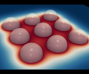
Apart from the single droplet dissolution, we also investigate convection in the situation of multiple droplets. Two different multiple droplet configurations, namely  $2\times 2$ and $3\times 3$ droplet arrays, have been explored. In both cases the droplet separation (measured from the edge of the droplet) equals half of the droplet initial radius (see figure 1 for the illustration of the set-up).

Figure 2. (a) Numerical results (red curve) for the droplet radius as a function of time for pure diffusion, compared to the EP theory (black dashed curve), with the correction term proposed by Popov (Reference Popov2005). (b) Nusselt number  $Nu$ versus time $t$ for the case of a constant-temperature spherical object, where the black squares denote the dataset given by Musong et al. (Reference Musong, Feng, Michaelides and Mao2016) and the blue curve is the result from our simulation.
3 Code verifications
Before presenting the results, we first verify our code against the analytical solution and the existing results from the literature. In the first part of the verification, we consider the dissolution of a sessile droplet with pure diffusion, i.e. we solve (2.2) with the advection term being switched off.
Epstein & Plesset (Reference Epstein and Plesset1950) considered a particular case for a single spherical bubble dissolving in the bulk fluid and analytically calculated the radius as a function of time. Later Popov (Reference Popov2005) extended this calculation to the case of a droplet sitting on a substrate at a given contact angle  $\unicode[STIX]{x1D703}$. However, Popov’s original model assumes the quasi-static behaviour, i.e. the time-dependent term on the right-hand side of (1.1) is eliminated. This assumption can greatly affect the numerical dissolution process, as shown by Zhu et al. (Reference Zhu, Verzicco, Zhang and Lohse2018). Therefore, in the verification, instead of directly using the mathematical expression in (1.2), we adopt the contact angle correction factor $f(\unicode[STIX]{x1D703})$ as proposed by Popov (Reference Popov2005) to the classical EP theory. In the case of $\unicode[STIX]{x1D703}=90^{\circ }$ and a single drop considered here, this just leads to the solution given in (1.1), and hereafter we still call this the EP theory for simplicity. Note that, due to the axial symmetry assumption in the calculation, it is only suitable for verifying the cases of a single droplet without convection, but not for the cases of multiple droplets.
Figure 2(a) shows the normalized droplet radius  $R/R_{0}$ versus the dimensionless time $\tilde{t}$ at $Ra=0.01$. It shows the excellent agreement between the EP theory (black dashed curve) and our numerical results (red curve) over the entire dissolution process. We remark that there is a little deviation at the final stage of the dissolution because the droplet size is getting smaller and the resolution of the Eulerian grid points in the Cartesian container becomes insufficient to resolve the droplet. However, if we focus on the lifetime of the droplet, which is the time for $R/R_{0}$ to reach zero, the error is less than 2 % and does not affect the final conclusion.
As second verification, we verify the code by simulating the convective flow. Musong et al. (Reference Musong, Feng, Michaelides and Mao2016) had used the IBM to study the heat transfer problem for an isolated isothermal sphere at various Grashof numbers,  $Gr=g\unicode[STIX]{x1D6FD}_{T}\unicode[STIX]{x1D6E5}_{T}d^{3}/\unicode[STIX]{x1D708}^{2}$, and Prandtl numbers, $Pr=\unicode[STIX]{x1D708}/\unicode[STIX]{x1D705}$, where $\unicode[STIX]{x1D705}$, $\unicode[STIX]{x1D6FD}_{T}$, $d$ and $\unicode[STIX]{x1D6E5}_{T}$ are the thermal diffusivity, thermal expansion coefficient, diameter of the sphere and the temperature difference between the heated surface and the ambient fluid. We modified our droplet dissolution code to deal with the heat transfer problem and compared with their result at $Gr=100$ and $Pr=0.72$. Figure 2(b) shows how the normalized heat flux (characterized by Nusselt number $Nu$ defined as the total heat flux across the surface of the sphere over the heat flux in the case of quiescent fluid) changes with time $t$. It can be seen that both the data taken from Musong et al. (Reference Musong, Feng, Michaelides and Mao2016) (black squares) and our numerical results (blue curve) agree with each other. The agreement is not only for the values after reaching the statistical steady state but also for the temporal evolution of $Nu$ over the entire heat transfer process.
4 Convective effects for single droplet dissolution
In this section we first show how the radius of a single surface droplet changes in time for different  $Ra$. Figure 3(a) shows the normalized radius $R(t)/R_{0}$ versus the normalized time $t/t_{EP}$ for various $Ra$, where $R_{0}$ and $t_{EP}$ represent the initial droplet radius and the reference lifetime based on the EP theory. For the cases of $0.1\leqslant Ra<10$, the curves almost collapse onto a single curve, and $R(t)/R_{0}$ drops to zero when $t\simeq t_{EP}$. This suggests that the droplet dissolution is purely diffusive and we regard those values of $Ra$ as small. However, when $Ra$ increases to 10, the buoyancy force becomes significant, as indicated by the (green) curve being below the collapsed one at small $Ra$. When $Ra$ further increases from 10 to 400, the lifetimes of the droplet are shortened progressively, as shown in figure 3(b), due to the increasing importance of the buoyancy force. For our largest explored $Ra(=400)$, the lifetime of the droplet even becomes half of $t_{EP}$, i.e. half of what it would be for pure diffusion.

Figure 3. (a) Time series for the radius of droplet  $R(t)$ for different $Ra$, where $R$ and $t$ are normalized by the initial droplet radius $R_{0}$ and the droplet lifetime estimated by EP theory $t_{EP}(Ra)$. (b) Lifetime of the droplet $\unicode[STIX]{x1D70F}$ normalized by $t_{EP}$ versus the Rayleigh number $Ra$. As discussed in § 3, the small deviation from $t_{EP}$ for small $Ra$ cases is due to the grid resolution issue because the droplet becomes too small at the final stage of dissolution.

Figure 4. Instantaneous Sherwood number  $Sh(t)$ versus the normalized time $t/\unicode[STIX]{x1D70F}(Ra)$ for different $Ra$, where $\unicode[STIX]{x1D70F}(Ra)$ is the droplet lifetime for the corresponding $Ra$. The dashed line corresponds to (4.2). The vertical dotted line indicates the time instant for the $Sh_{inst}$ shown in figure 5.

Figure 5. (a) Sherwood number  $Sh$ versus the Rayleigh number $Ra$. For the numerical results, the Sherwood number is defined at the instant when the $Sh$ curve is still relatively flat, as shown in figure 4, which is represented by $Sh_{inst}$. For details, we refer to the main text. (b) Sherwood number $Sh$ compensated with $Ra^{1/4}$ versus $Ra$. The experimental data from Dietrich et al. (Reference Dietrich, Wildeman, Visser, Hofhuis, Kooij, Zandvliet and Lohse2016) have also been included. Note that the data compare one-to-one and no fitting or scaling parameter is involved.
Another important quantity to be examined is the mass flux, which in dimensionless form is expressed as the following Sherwood number:
 $$\begin{eqnarray}Sh=\frac{\langle {\dot{m}}\rangle _{A}R}{Dc_{s}}=\frac{\unicode[STIX]{x1D70C}_{d}}{c_{s}}\frac{1}{\sqrt{RaSc}}\tilde{R}\frac{\text{d}\tilde{R}}{\text{d}\tilde{t}}.\end{eqnarray}$$
 Here  $\langle {\dot{m}}\rangle _{A}$ is the mass flux averaged over the droplet surface and $Dc_{s}/R$ is the reference mass flux for the case of the surface droplet (of $90^{\circ }$ contact angle) dissolving diffusively and quasi-statically. In (4.1) the expression for $Sh$ is further rewritten to connect it to the (dimensionless) radius shrinkage $\text{d}\tilde{R}/\text{d}\tilde{t}$ and the control parameters $Ra$,
$Ra$,  $Sc$ and $\unicode[STIX]{x1D70C}_{d}/c_{s}$.
Given the temporal evolution of the droplet radius, as shown in figure 3(a), the corresponding temporal evolution of  $Sh$ can be computed (see figure 4). Since the lifetimes for various $Ra$ differ a lot from each other, we normalize the time $t$ by the respective lifetime of the droplet $\unicode[STIX]{x1D70F}(Ra)$ in each case for better comparison. First, for $0.1\leqslant Ra<10$, we again observe that the curves collapse onto each other. Moreover, $Sh$ changes slightly with time for these cases throughout the entire dissolution process. Using $Ra=0.1$ as an example, the value of $Sh$ is approximately 1.3 at $t=0.1\unicode[STIX]{x1D70F}$, and then $Sh$ decreases gradually to 1 until the droplet is completely dissolved. In order to understand this trend, we substitute the analytical solution (1.1) given by the EP theory into the expression for $Sh$ in equation (4.1). This gives $Sh(t)$ for the diffusion-dominated case as
 $$\begin{eqnarray}Sh=1+\frac{R}{(\unicode[STIX]{x03C0}Dt)^{1/2}}.\end{eqnarray}$$
 It can be seen that the correction leads to an additive term  $R/(\unicode[STIX]{x03C0}Dt)^{1/2}$ to the purely diffusive case under the quasi-static approximation where $Sh=1$. The significance of this term diminishes when $t$ gets larger and $Sh$ approaches 1 eventually. However, on increasing $Ra$ from $Ra=10$, the expression (4.2) does not hold any more due to the increasing influence of buoyancy. Upon increasing $Ra$, we observe that the magnitude of $Sh$ becomes larger. Furthermore, taking the largest $Ra$ ( $=400$) as an example, one observes that the mass flux remains at a constant value ( $Sh\sim 3.8$) over a large portion of the dissolution time, until, near the final stage of the dissolution, the value of $Sh$ decreases rapidly. The decrease of the mass flux can be understood by the smaller effective Rayleigh number caused by the reduced droplet size, such that the effect of buoyancy is weaker.
Next, we examine the dependence of the dimensionless mass flux  $Sh$ on $Ra$. Notice from figure 4 that $Sh$ only slightly decreases for $t\leqslant 0.5\unicode[STIX]{x1D70F}$ but then sharply decreases near the final stage of dissolution. It leads us to define an instantaneous Sherwood number $Sh_{inst}$ at the instant when the $Sh$ curve is still relatively flat. Here, the moment of $t=0.2\unicode[STIX]{x1D70F}$ is chosen to calculate $Sh_{inst}$ (indicated by the vertical dotted line in figure 4). Note that our conclusion is not sensitive to the choice of the specific time, since $Sh$ does not change much near $t=0.2\unicode[STIX]{x1D70F}$. In figure 5(a), it can be seen that, on increasing $Ra$, there is a clear transition of $Sh(Ra)$ scaling from a constant to $Ra^{1/4}$. This reflects that the droplet dissolution changes from a diffusively dominated process to a convectively dominated process because of the increasing significance of buoyancy. To have a better insight into the scaling change, we further plot $Sh$ compensated with $Ra^{1/4}$ in figure 5(b), which indeed clearly reveals the $1/4$ scaling exponent.
We now compare our numerical results with the recent experimental results by Dietrich et al. (Reference Dietrich, Wildeman, Visser, Hofhuis, Kooij, Zandvliet and Lohse2016), who studied a long-chain alcohol droplet dissolving in water and also found an enhanced dissolution rate due to the occurrence of convective flow. In figure 5, we plot the experimental data points from Dietrich et al. (Reference Dietrich, Wildeman, Visser, Hofhuis, Kooij, Zandvliet and Lohse2016) together with our numerical data for comparison. First, from their experiment, data points from different alcohols have collapsed onto almost the same curve, and this curve also displays the change of scaling exponent to  $1/4$ on increasing $Ra$. As explained in Dietrich et al. (Reference Dietrich, Wildeman, Visser, Hofhuis, Kooij, Zandvliet and Lohse2016), this scaling can be understood as follows: For large enough $Ra$, there is a concentration boundary layer developed on top of the droplet surface. The thickness of this boundary layer $\unicode[STIX]{x1D6FF}_{c}$ has the Pohlhausen power-law dependence with $Ra$, which is $\unicode[STIX]{x1D6FF}_{c}/R\sim Ra^{-1/4}$ (Pohlhausen Reference Pohlhausen1921; Schlichting & Gersten Reference Schlichting and Gersten2016). By using $\unicode[STIX]{x1D6FF}_{c}$ as the typical length scale for estimating the mass flux, which is $\langle {\dot{m}}\rangle _{A}\sim Dc_{s}/\unicode[STIX]{x1D6FF}_{c}$, one can obtain $Sh\sim Ra^{1/4}$. Apart from the scaling change, our numerical results also confirm the value of the transitional Rayleigh number, $Ra_{t}\simeq 12.1$, found in the experiments.

Figure 6. Instantaneous snapshots for the concentration field together with velocity vectors for  $Ra=0.1$ (a) and $Ra=100$ (b) in the case of a single surface droplet. The location of this vertical cross-section is taken in the middle of the droplet (also the middle of the domain). The interface of the droplet at different time instants is indicated by the solid line. Movies can be seen in the supplementary material available at https://doi.org/10.1017/jfm.2020.175.
To further characterize the two different dissolution regimes, we compare the respective flow morphologies. Figure 6 shows instantaneous slices of the concentration field taken at the vertical mid-plane. We visualize the time evolution of the concentration by showing the field at different time instants for two different  $Ra$. First, for small $Ra$ ( $=0.1$), as shown in the upper panels, the dissolution happens basically through diffusion, and one can see that the dissolution rate is almost the same in all directions. On the contrary, this isotropic mass transfer is broken for larger $Ra$, specifically for $Ra\geqslant 10$. For example, at $Ra=100$, as shown in the lower row, the vertical velocity above the droplet strengthens significantly so that the concentration field is mainly displaced upwards rather than sidewards. Near the initial stage of dissolution at $t=0.05\unicode[STIX]{x1D70F}$, one can observe the emission of a concentration plume from the top of the droplet. When the solute dissolves into water, it results in less dense liquid in the denser surrounding, and such an unstable stratified region leads to the emission of plumes. This mechanism of concentration plume emission is similar to the thermal plume emission in Rayleigh–Bénard convection, which is a classical model for thermal convection with a fluid layer heated from below and cooled from above (Shang et al. Reference Shang, Qiu, Tong and Xia2003; Ahlers, Grossmann & Lohse Reference Ahlers, Grossmann and Lohse2009). As the droplet continues to dissolve, a long tail of the plume remains connected to the top of the droplet, but of a smaller size, until the droplet is completely dissolved.
5 Convective effects for multiple droplet dissolution
Given the good agreement with the experimental results, we now extend our numerical study to the case of multiple droplets. Two different multiple droplet configurations are studied, namely  $2\times 2$ and $3\times 3$ droplet arrays. To compare the different dissolution dynamics in the diffusion-dominated and convection-dominated regimes, figure 7(a) shows the top view (cutting near the bottom plate on which the droplets are placed) of the concentration fields for $Ra=0.1$ and $Ra=100$ using the $3\times 3$ array as an example. To also have a quantitative comparison, figure 7(b,c) shows the normalized radius $R/R_{0}$ versus the normalized time $t/t_{EP}$, where $t_{EP}$ is the lifetime estimated by the EP theory for a single droplet.

Figure 7. (a) Top view for the instantaneous concentration fields taken at the layer close to the bottom plate for  $Ra=0.1$ and $Ra=100$. To guide the eye, the interfaces of the droplets are also outlined by the grey surfaces. (b,c) Time series for the normalized radius $R(t)/R_{0}$ versus the normalized time $t/t_{EP}$ for $Ra=0.1$ in (b) and $Ra=100$ in (c). Here $R_{0}$ and $t_{EP}$ denote the initial droplet radius and the single droplet lifetime estimated by the EP theory. To denote the droplets at different topological locations, they are indexed with the number 1, 2 and 3 as indicated in (a) for $t=0.1\unicode[STIX]{x1D70F}_{1}$.
For  $Ra=0.1$ the collective dissolution leads to much faster accumulation of solute among the droplets as compared to the single droplet dissolution. This is the so-called shielding effect (Carrier et al. Reference Carrier, Shahidzadeh-Bonn, Zargar, Aytouna, Habibi, Eggers and Bonn2016; Laghezza et al. Reference Laghezza, Dietrich, Yeomans, Ledesma-Aguilar, Kooij, Zandvliet and Lohse2016; Bao et al. Reference Bao, Spandan, Yang, Dyett, Verzicco, Lohse and Zhang2018; Michelin et al. Reference Michelin, Guérin and Lauga2018; Wray et al. Reference Wray, Duffy and Wilson2019). The existence of the neighbouring droplets tends to lower the concentration gradient experienced by all the droplets and results in a decreased dissolution rate. Another feature of the shielding effect is that the dissolution of the multiple droplets follows the sequence $\unicode[STIX]{x1D70F}_{3}<\unicode[STIX]{x1D70F}_{2}<\unicode[STIX]{x1D70F}_{1}$, where $\unicode[STIX]{x1D70F}_{i}$ is the lifetime for the $i$th droplet – see figure 7(a) for $t=0.1\unicode[STIX]{x1D70F}_{1}$ for the locations. Indeed, both the qualitative visualization in figure 7(a) and the radius time series in figure 7(b,c) confirm such a sequence of dissolution. Moreover, we show that, for all the droplets, they dissolve slower than the single droplet case with pure diffusion.
In contrast, the dissolution pattern changes significantly when convection plays a role. The second row of figure 7(a) shows the concentration field for  $Ra=100$. From the footprint of the concentration field at $t=0.4\unicode[STIX]{x1D70F}_{1}$, it shows that the solute tends to flow towards the central droplet. Apart from the change in the concentration distribution, figure 7(c) further shows that the dissolution time of droplet 3, $\unicode[STIX]{x1D70F}_{3}$, becomes comparable to that of droplet 2, $\unicode[STIX]{x1D70F}_{2}$. This feature is non-trivial and opposes the expectation from the shielding effect.

Figure 8. Instantaneous snapshots for the concentration field together with velocity vectors in the vertical mid-plane for  $Ra=100$ in the case of the $3\times 3$ multiple droplet array. Note that the mid-plane cuts through the centre of droplets 1 and 2. Snapshots at different time instants indicate the formation of a single, larger plume from individual plumes. The time $\unicode[STIX]{x1D70F}_{1}$ represents the lifetime of the central droplet (droplet 1). A movie of this process can be seen in the supplementary material.
To understand this counter-intuitive result, we thus explore the morphological changes in the flow caused by the significant influence of convection for multiple droplets. Figure 8 visualizes the concentration field at the vertical mid-plane for  $Ra=100$. At the initial stage of dissolution ( $t=0.02\unicode[STIX]{x1D70F}_{1}$), we observe plumes emitted mainly from the two side droplets. For the central droplet, the concentration gradient is largely diminished due to the existence of the neighbouring droplets. Therefore, at $t=0.03\unicode[STIX]{x1D70F}_{1}$, we find that the upward velocity above the central droplet is weaker than that above the side droplets. However, instead of just moving upwards, the concentration plumes tend to merge together above the central droplet. Eventually, the merging event results in a single larger plume moving vertically upwards at $t=0.04\unicode[STIX]{x1D70F}_{1}$. Finally, at $t=0.05\unicode[STIX]{x1D70F}_{1}$, the narrow tail of the plume is maintained and this morphology remains for the rest of the dissolution process until the droplets are completely dissolved.
So far, we have revealed that the plumes need not be individual but that they can interact with each other, leading to a new mechanism for collective droplet dissolution through merging of plumes. This somewhat mimics the daily-life example (in the days of Michael Faraday) of two merging flames from two nearby candles: as the fluid in the middle of the two candles receives the strongest heating from the two flames, there is a stronger updraft between the two candles and the merged flame can reach a higher position. Likewise, a more energetic merged plume can form for multiple droplet dissolution which enhances the mass transfer. We cite Michael Faraday’s ‘Chemical History of a Candle’ (Faraday Reference Faraday1861): ‘There is no better, there is no more open door by which you can enter into the study of natural philosophy than by considering the physical phenomena of a candle.’ Here, we have recognized the similarity between the candle melting and the droplet dissolving in their collective behaviours, and therefore it enlightens the research on droplet dissolution. In the analogous case – a bubble – Lhuissier & Villermaux (Reference Lhuissier and Villermaux2012) have also found that rich fluid mechanics can be learnt through studying the bursting bubble similar to the study of the melting candle.
To demonstrate the effect of the merging event on the lifetime of the droplets, figure 9(a,c) shows the normalized lifetime  $\unicode[STIX]{x1D70F}/\unicode[STIX]{x1D70F}_{single}$ versus $Ra$ for $2\times 2$ and $3\times 3$ droplet arrays. Here the lifetimes $\unicode[STIX]{x1D70F}$ have been normalized by the respective reference value $\unicode[STIX]{x1D70F}_{single}(Ra)$, which is the $Ra$-dependent lifetime corresponding to the single droplet case. In addition, we also plot the maximum vertical velocity $w_{max}$ at the mid-height versus $Ra$ for both arrays in figure 9(b,d). Again, the vertical velocity has been normalized by the value obtained from the respective single droplet case, $w_{max,single}(Ra)$, which also depends on $Ra$, of course. Here we only consider the magnitude of the vertical velocity because we focus on the enhancement of mass transfer in the buoyancy-driven flow where gravity is acting in the vertical direction.

Figure 9. (a,c) Normalized droplet lifetime  $\unicode[STIX]{x1D70F}/\unicode[STIX]{x1D70F}_{single}$ in the case of multiple droplets versus $Ra$ for $2\times 2$ droplet array in (a) and $3\times 3$ droplet array in (c). Here $\unicode[STIX]{x1D70F}_{single}$ represents the lifetime in the case of a single droplet. The indices represent the droplets from different locations, as indicated in figure 7(a). The inset in (c) shows that the multiple droplet lifetime can be shorter than the single droplet lifetime for large enough $Ra$. It also shows the minimal normalized lifetime at $Ra=20$. (b,d) Maximum vertical velocity $w_{max}$ normalized by that in the single droplet case, $w_{max,single}$, versus $Ra$ for the $2\times 2$ droplet array in (b) and the $3\times 3$ droplet array in (d). Both show a pronounced maximum around $Ra=4$.

Figure 10. Horizontal profiles of the normalized vertical velocity  $w/w_{max}$ for various $Ra$, where $w_{max}$ is the maximum value of the respective profile. The dimensionless horizontal coordinate is represented by $\tilde{x}$ and we plot the vertical dashed line to show the locations of droplet 2 (blue) and droplet 1 (black).
For the  $2\times 2$ droplet array, all four droplets are topologically equivalent and therefore figure 9(a) only shows one set of data. When $Ra\leqslant 1$ the normalized dissolution time $\unicode[STIX]{x1D70F}/\unicode[STIX]{x1D70F}_{single}$ is not sensitive to the change of $Ra$ and the multiple droplets dissolve slower than the single droplet with $\unicode[STIX]{x1D70F}=1.5\unicode[STIX]{x1D70F}_{single}$. However, $\unicode[STIX]{x1D70F}/\unicode[STIX]{x1D70F}_{single}$ decreases with increasing $Ra$ when $Ra$ becomes larger than 1. As $Ra$ increased up to around 40, the lifetimes of the multiple droplets become comparable to that of the single droplet. With further increasing $Ra$, the value of $\unicode[STIX]{x1D70F}/\unicode[STIX]{x1D70F}_{single}$ again becomes insensitive to the change of $Ra$ and stays at around 1. This reduction in the lifetime $\unicode[STIX]{x1D70F}$ compared to $\unicode[STIX]{x1D70F}_{single}$ can be explained by the enhanced vertical velocity shown in figure 9(b). Owing to the merging of the concentration plumes, the maximum velocity $w_{max}$ is considerably larger than that of the single droplet case, $w_{max,single}$.
Likewise, for the  $3\times 3$ droplet array, the trend of $\unicode[STIX]{x1D70F}/\unicode[STIX]{x1D70F}_{single}$ is similar to that for the $2\times 2$ array but there is a stronger collective effect. In this $3\times 3$ array, there are three topologically different droplets. We display their lifetimes versus $Ra$ in figure 9(c). From that, we can basically classify three different regimes based on the slopes of the curves: in regime I, where $Ra\leqslant 1$, the normalized lifetime remains unchanged with increasing $Ra$. In this parameter range, the droplet dissolution is still limited by diffusion and the shielding effect dominates the dissolution process. In the range $1\leqslant Ra\leqslant 10$, regime II, we recall that the single droplet dissolution within this $Ra$ range should be diffusion-dominated. However, here we observe the decrease of the normalized lifetime with increasing $Ra$, which reflects the increased influence of the buoyancy force due to the collective droplets. Indeed, figure 9(d) also shows the significant enhancement in the vertical velocity in this $Ra$ range. In regime III, $Ra\geqslant 10$, we observe that the normalized lifetime of the outermost droplet 3 has reached a plateau where $\unicode[STIX]{x1D70F}/\unicode[STIX]{x1D70F}_{single}$ stays at around 1. To inspect the behaviour of $\unicode[STIX]{x1D70F}/\unicode[STIX]{x1D70F}_{single}$ at the transition from regime II to III in more detail, we zoom in to the region around $Ra=10$ as shown in the inset of figure 9(c). We observe that there is an optimal case at $Ra=20$ where the lifetime of droplet 3 becomes even shorter (approximately 5 %) than that in the case of a single droplet. This in fact holds for the whole range $10\leqslant Ra\leqslant 100$.

Figure 11. Time series of Sherwood number  $Sh$ versus the normalized time $t/\unicode[STIX]{x1D70F}$, where $\unicode[STIX]{x1D70F}$ is the lifetime of the droplet at $Ra=0.1$ in (a) and $Ra=20$ in (b). For each $Ra$, the blue curve represents the case of single droplet while the black curve represents the outermost droplet (droplet 3) in the case of the $3\times 3$ droplet array. In (b), the vertical cross-section of the concentration fields at different time instants is also shown. Depending on the moment in time, the collective dissolution is either stronger or weaker than that of the isolated droplet.
Given that larger  $Ra$ represent a relatively stronger buoyancy effect, the above observation indeed raises the question of why there is an optimal $Ra$ at which there is a maximum reduction in the droplet lifetime compared to the single droplet case. We explain it by showing the horizontal profiles of the vertical velocity $w$ (normalized by the maximum vertical velocity $w_{max}$) taken at the mid-height in figure 10. The profiles are taken at the instant when droplet 2 is half of its initial radius. For all $Ra$, the profiles exhibit a maximum at the centre ( $\tilde{x}=0$, where the entire horizontal extent ranges from $\tilde{x}=-8$ to $\tilde{x}=8$) and the profiles are symmetric about the central line. A key feature is that, when $Ra$ increases from 4 to 400, the profiles become narrower, as noticed by the half-maximum of the profiles. The consequence is that at the location of the droplet 2, which is either $\tilde{x}=-3$ or $\tilde{x}=3$, the value of $w/w_{max}$ actually decreases with increasing $Ra$. This suggests that, although the effect of buoyancy is stronger at larger $Ra$, the vertical velocity experienced by the edge droplets can be diminished due to the shrinkage in width of the upward-moving merged plume.
To better understand the optimal case, for which the normalized dissolution time is minimal as a function of  $Ra$, we examine the time series of $Sh$. For comparison, we begin with the time series for the case of $Ra=0.1$ in figure 11(a). It shows that, for the outermost droplet (droplet 3), the value of $Sh$ during the entire dissolution process is lower than that of the single droplet dissolution, thanks to the shielding effect. However, at the optimal case of $Ra=20$, figure 11(b) shows that the value of $Sh$ for the outermost droplet is not always smaller than that in the single droplet case: First, when $t$ is below $0.1\unicode[STIX]{x1D70F}$, the value of $Sh$ for droplet 3 is lower than that of the single droplet. By the corresponding concentration field over that period of time, one can see that the individual concentration plumes just emit from the droplets without merging at this early stage. However, there is a cross-over around $t=0.1\unicode[STIX]{x1D70F}$ where the individual plumes are observed to just merge into a single plume. After that, $Sh$ for the outermost droplet remains larger than that for the single droplet case. The result again confirms that it is the merging of plumes that leads to the enhancement of the dissolution rate.
Note that Laghezza et al. (Reference Laghezza, Dietrich, Yeomans, Ledesma-Aguilar, Kooij, Zandvliet and Lohse2016) have also experimentally observed the enhancement of the mass flux for collective and convective dissolution. Indeed, they find that the dissolution time of the droplets at the edges can reduce to values below that of a single isolated droplet. Thanks to our numerical work, this dissolution enhancement can now be linked to the merging of the plumes.
6 Concluding remarks and outlook
In summary, we numerically modelled and investigated convective droplet dissolution over a wide range of  $Ra$ from 0.1 to 400 with $Sc$ being fixed at 1200 and $c_{s}/\unicode[STIX]{x1D70C}_{d}$ fixed at 0.027 (representing 1-pentanol in water). For all our explored cases, we consider the constant contact angle dissolution mode with contact angle being fixed at $90^{\circ }$. As the starting point, we verified our code for the pure diffusive droplet dissolution by comparing with the analytical results by Epstein & Plesset (Reference Epstein and Plesset1950) and Popov (Reference Popov2005). We then provided further verification to show our proper implementation of the convective term in our code by comparing to the heat flux data in a heat transfer problem. Then we used this numerical code to simulate droplet dissolution for both the single droplet and multiple droplets scenarios.
For a single droplet, we showed that the Sherwood number  $Sh$ stays at around 1 regardless of $Ra$, provided that $Ra$ is smaller than 10. However, $Sh$ undergoes a transition to $Sh\sim Ra^{1/4}$ when $Ra$ is above 10. Our numerical results agree with the previous experimental results by Dietrich et al. (Reference Dietrich, Wildeman, Visser, Hofhuis, Kooij, Zandvliet and Lohse2016) for single droplet dissolution, in which the transition from a constant value to $Sh\sim Ra^{1/4}$ was also found at the same $Ra_{t}\simeq 10$. Moreover, we gained insight into the change in the flow morphologies by comparing the concentration fields in the different regimes. An essential feature of the convective regime $Sh\sim Ra^{1/4}$ is that there is a clear emission of concentration plumes above the droplet, which carries large amount of solute away from the droplet. Our results thus illustrated, from both the $Sh$ behaviour and the flow morphologies, how, with increasing $Ra$, the dynamics of droplet dissolution changes from diffusion-dominated to convection-dominated.
When we extended the geometry to multiple droplets, richer phenomena could be observed. With multiple droplets, the traditional view was that the shielding effect can lead to the large suppression of mass flux due to the smoothened concentration gradient around the droplets. However, the basis of the shielding effect is that the diffusion dominates the dissolution process. Here, with the significant role of convection for large  $Ra$, we first showed that the outermost and the second outermost droplets (in $3\times 3$ droplet array) have comparable lifetimes, which opposes the view of a shielding effect. Thanks to the numerical simulations, we further revealed that the concentration plumes can merge into a large, single plume, which is the mechanism leading to the collective enhancement of droplet dissolution. With the help of plume merging, the magnitude of vertical velocity is greatly increased and the dissolution time for the outermost droplet can be shorter than that of a single droplet by 5 % (at $Ra=20$) for our explored parameter range. Based on qualitative experimental observations, Laghezza et al. (Reference Laghezza, Dietrich, Yeomans, Ledesma-Aguilar, Kooij, Zandvliet and Lohse2016) had also reported the enhanced mass flux for multiple droplet dissolution. Here, we understand this enhancement by linking it to the newly found mechanism – plume merging. Another non-trivial result is the existence of an optimal $Ra$. We have provided an explanation by showing that the updraft associated with the large plumes becomes narrower for larger $Ra$. It eventually limits the mass flux of the droplets near the edge, as those droplets are less affected by the upward-moving merged plume.
To the best of our knowledge, our study is the first of its kind to provide a detailed physical quantification of the convective collective droplet dissolution problem using numerical simulations. The present study reveals a variety of physical effects thanks to the interplay between the two mechanisms, namely the shielding effect and the merging of concentration plumes. Our findings have thus provided a more comprehensive picture of the collective behaviour of multiple droplet dissolution.
Many questions remain open. For example, how does the separation between multiple droplets influence the relative strength of the two mechanisms? How do things change for different contact angles  $\unicode[STIX]{x1D703}\neq 90^{\circ }$, or even for different dissolution modes, namely for the constant contact radius mode rather than the constant contact angle mode as employed here? Another question is on the convective effect for negative Rayleigh number, i.e. for droplets consisting of denser liquid dissolving in a less dense host liquid. As we have demonstrated some non-trivial and at first sight counter-intuitive results in collective and convective droplet dissolution, it is clearly worthwhile to further explore the parameter space of this system.
Acknowledgements
We greatly appreciate valuable discussions with X. Zhang, A. Prosperetti and E. Villermaux. We acknowledge the support from ERC-Advanced Grant under the project no. 740479. K.L.C. also acknowledges Croucher Foundation for the Croucher Fellowships for Postdoctoral Research. We acknowledge that the results of this research have been achieved using the DECI resource Kay based in Ireland at Irish HPC Centre with support from the PRACE. We also acknowledge PRACE for awarding us access to MareNostrum at the Barcelona Supercomputing Centre (BSC) under PRACE project no. 2017174146 and JUWELS at the Jülich Supercomputing Centre. This work was also partly carried out on the national e-infrastructure of SURFsara with the support of the SURF Cooperative.
Declaration of interests
The authors report no conflict of interest.
Supplementary movies
Supplementary movies are available at https://doi.org/10.1017/jfm.2020.175.


 Open access