


Introduction
Stream-flow data from most Norwegian river gauging stations are collected by the hydrological Department within the Norwegian Water Resources and Energy Administration. Some data series, comprising daily run-off figures for selected streams, cover more than 100 years, but the majority of water discharge data were collected during the last few decades. To make a good plan for a hydro-electric power station, it is vital to have a statistically-reliable hydrologic background to select optimal turbine and generator installations. Thus a 30-year observation period of daily run-off measurements is normally required.
For many mountain streams, this requirement may be difficult to fulfill, due to the fact that remote mountain areas were, in the past, not regarded as important for hydrological studies. Gauging stations were not installed until relatively recently, when it became clear that the increased demand for energy required hydro-electric developments also in these remote and almost uninhabited areas. However, in some cases data are available also from some old hydrometric stations, so that the short series can be supported by the old ones via correlation models.
A more serious problem is the fact that almost all existing data from mountain basins were collected in a period of general glacier shrinkage, i.e. during years when the glaciers supplied amounts of “extra” melt water to the mountain streams. Thus, their run-off has been larger than during previous periods when glaciers were in a more or less steady state.
It has proved very difficult to find out how large this glacier contribution has been. In the planning procedure for power stations, it is vital to find a realistic figure for “normal run-off”, i.e. a figure which may be valid for the lifetime of the power station. This “normal” figure is defined as the long-term average without glacier influence or with all glaciers being in a steady state.
One way to find this important figure is to carry out detailed mass-balance investigations on glaciers within the given basin. This has also been done – a number of glaciers were selected for such studies in the 1960s and 1970s. Due to many years of negative glacier mass balance, a reduction has now been made of the actually-observed discharge figures and we have obtained a much more realistic base for future power developments in Norway (Reference ØstremØstrem, 1973).
Another method, which has now been tested, is a repeated glacier mapping programme, comprising periods of general glacier retreat. This is a new way to provide data to adjust actual measured water run-off in glacier-fed streams, i.e. to produce the above-mentioned “glacier-behaviour-corrected” figures. It is quite obvious that a power station cannot be dimensioned for an expected continued glacier retreat in the future, relying on extra amounts of water provided by annual negative mass balance. This would be the case if the raw hydrological data from glacier-fed rivers were used directly in the planning procedure.
River Discharge Measurements in Norway
The longest series of water discharge measurements dates back to 1845, when the first gauging station was installed in Norway. The network of hydrometric stations has been increasing, particularly since the 1950s, and presently some 1200 gauging stations are operating. (Catalogues of available data from the entire network are issued by the Hydrological Department, see for example NVE 1983.) So there is a good hydrological basis for calculations of average annual flow, at least in non-glacierized areas. However, already in the years 1900-1910, several stations were installed in rivers which are more or less glacier-influenced. About ten such stations in glacier-fed rivers have been continuously running for more than 75 years, giving daily discharge data for rivers with an appreciable amount of glaciers in their basins. For example, the hydrometric station at Loen (draining 78 km2 glacier area, which is 30% of its total basin) has been running since 1901. Similarly, the hydrometric station at Olden (draining 76 km2 glacier area which is 36% of its total basin) has been running since 1902. The station at Breimsvatn, which has been operating since 1900 has a glacier coverage of 12% or 71 km2.
The hydrographs from these stations show appreciable annual variations which are partly due to variations in annual precipitation and partly due to glacier influence. It has, however, proved extremely difficult to differentiate between these two sources of annua! discharge variations. There are some long meteorological observation series available and it is obvious that glacier-fed rivers carry more water in dry, hot summers than other streams, but to find the quantitative relation has been, so far, extremely difficult.
Glacier Mass Balance
The earliest mass-balance investigations in Norway were made on the valley glacier, Storbreen, in Jotunheimen by the Norwegian Polar Research Institute (Reference LiestølLiestøl 1967, Reference Liestøl1984). This observation series is, in fact, the second longest of its kind in the world; it started in 1948 and is still being maintained. This means that we have at least one long series of data showing glacier behaviour during the last 37 years. From this, some conclusions can be drawn concerning the above-mentioned corrections to be made in existing data series on river discharge.
However, one single glacier (5.4 km2) cannot be representative for all the other glaciers (2745 km2) in the country (Reference Østrem and ZieglerØstrem et.al. 1969, Reference Østrem, Haakensen and Melander1973), Therefore, the Hydrological Department started mass-balance investigations on several glaciers in various parts of Norway during the 1960s, The longest continuous series is that from Nigardsbreen, an outlet glacier from the ice cap Jostedalsbreen, in south-western Norway (Reference Østrem, Liestøl and WoldØstrem et.al. 1976). Investigations started there in 1962 and will be continued also in the future. It is intended to continue all long observation series and, most probably, to include more glaciers in the observational programme. This will be done in connection with the planning of future power developments in glacier-rich areas. However, for such planning, much longer series of glaciological data would be desirable.
Glacier Mapping and Glacier Variations
Corrections of discharge data for glacier behaviour have been made only for the last 10-20 years and only for certain basins, due to relatively short series of mass-balance observations on representative glaciers. On the other hand, air photography has been carried out for a longer period – in principle since the 1950s - so attempts have now been made to use the oldest available air photographs of selected glaciers to form a basis for a topographical comparison betwen the “old” glacier surface and the corresponding glacier surface today.
This means that, if repeated air photography and detailed maps of the glacier surface are available in each case, a simple subtraction can be made to calculate the decrease in surface elevation. Thus it is possible to calculate the volume of additional melt water which has been delivered to the glacier-fed streams.
Consequently, the actually-observed river discharge can be reduced correspondingly to provide “glacier-corrected” hydrological data for the planning of water power installations.
When the calculations are made, it is assumed that the total glacier shrinkage in the intervening years İs evenly distributed in time. This assumption is obviously not glaciologically correct, but for a calculation of, say, 30 years of average discharge the simplification has no influence on the final result. From the long series of mass-balance observations obtained at Storbreen, mentioned above, and from similar studies at Storglaciären, in northern Sweden, dating back from 1946, it is quite clear that there has been an almost continuous annual glacier shrinkage since the 1950s. Some odd years of glacier growth have been observed (e.g. 1962 when Nigardsbreen added 2 m of water equivalent to its entire surface), but the general trend has been glacier retreat for most of the glaciers under study. Only very recently, some of the glaciers in maritime areas show a tendency to grow again. This confirms the need for corrected run-off data for future planning.
Repeated glacier mapping
During the 1960s, it proved necessary to produce large-scale, detailed maps for those glaciers which were selected for mass-balance investigations. The selection of glaciers was made in accordance with current plans for hydro-electric developments in various parts of Norway.
At an early stage, three glaciers in southern Norway were selected for detailed mass-balance investigations, and it became essentia! to have good glacier maps available in printed form for this work. Consequently, special air photography was done to produce the maps of Nigardsbreen and Tunsbersdalsbreen. outlet glaciers from the Jostedalsbreen Ice Cap. Photographs were taken in 1964 and maps were issued in the following years. Similarly, a map of Helistueubreen in the Jotunheimen mountain area was issued in 1965 (Fig.1).
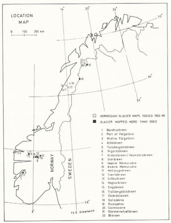
Fig. 1 Index map showing the location of glacier maps issued in Norway. Areas indicated by black squares are covering glaciers which are mapped more than once.
The first map of Hellstugubreen was based upon terrestrial photography and plane-table measurements, so soon it became clear that special air photography would be necessary to produce a more accurate map. Photographs were taken in 1968 and a map produced in 1969 – but unfortunately only blue-line prints were available - so, when further air photography was performed in 1980, a new map was constructed and this map was printed in four colours. It is therefore now possible to study variations in glacier volume with a high accuracy, particularly between 1968 and 1980. The result is shown in Table I.
Table 1 Glaciers where Repeated Mapping was used to Calculate Volume Change to Produce Hydrological Data (“Glacier-Corrected Run-Off”)
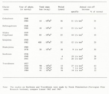
For the outlet glacier, Nigardsbreen, it also became clear that a great change had taken place since the 1964 air photography. New verticals were therefore taken in 1974, resulting in a map printed in 1975 in four colours. However, due to some missing areas on the 1964 verticals and because the 1974 pictures showed some of the firn areas covered by fresh snow, it is not possible, in this case, to make a complete calculation of glacier shrinkage. New photographs were taken in August, 1985, and these could be compared to good photographs taken in 1966 by the Geographical Survey of Norway, for the construction of a new topographic map of the area. This study will be of extremely high interest because detailed mass-balance investigations have been performed on Nigardsbreen since 1962. Thus, it will be possible also to compare the two methods of determining the total glacier shrinkage, i.e. the use of multi-temporal glacier maps and the traditional field observations of mass balance.
The most recent example of the use of repeated glacier mapping is the small cirque glacier, Grâsubreen, in the Jotunheimen mountain area. Good air photographs were taken and detailed glacier maps were constructed in 1968 and 1985. Here, it has been shown by Haakensen (1985) that both direct annual mass-balance measurements and glacier mapping seem to be necessary, in certain cases, to calculate the extra amount of melt water delivered by glacier shrinkage. The main reason is that this glacier is of the sub-polar type — certain parts of the annual melt water re-freeze on the glacier surface, and this process has inter-fered with the ablation observations.
A more recent set of repeated air photography, resulting in two good glacier maps, is that from Midtre Folgefonni, based upon verticals from 1959 and 1981. The map is printed in four colours and it was given the typical cartographic style which has developed during the last two decades in Norway, see next section.
A relatively small glacier, Riukojietna, a little ice cap in northern Norway, was photographed in 1960 and in 1978 and a special map was produced, depicting the glacier surface on these two occasions. As in the examples mentioned above, valuable hydrological information resulted from the map comparisons (Table I).
Multi-temporal glacier mapping
In one particular case it has been possible to compare several maps of the same glacier, based upon air photographs taken on various occasions. The glacier Salajekna, a somewhat complicated system of valley glaciers on the Norwegian-Swedish border in northern Scandinavia, was the subject of air photography missions from both countries, The earliest-known modern vertical air photography of a glacier was, in fact, that made over Salajekna, in 1950, by Widerøe’s Flyveselskap. This large-scale photography was intended mainly for mining engineering purposes, but because a great number of pictures covered the glacier, we were able to produce a detailed glacier map from it.
Only a few years later, in 1957-58, it was decided to take air photographs of the entire border between Norway and Sweden. Consequently, the glacier Salajekna was again photographed and the pictures were sufficiently good to produce another glacier map. Finally, the mapping Agencies in Norway and Sweden took photographs in 1971 and 1980-82, respectively, to produce new topographic maps. Consequently, no less than four different glacier maps could be produced, making possible a comparison between the glacier outline as well as the surface variations during the last 30 years. These four maps are printed together on the same sheet of paper and are enclosed with this article. The results of some comparisons are shown on the reverse side of the map, together with old drawings and photographs.
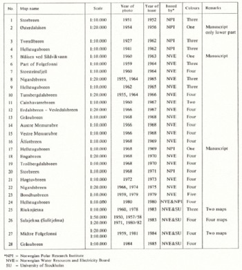
A list of glaciers, where the “topographic method” has been used to produce hydrological data, is given in Table I. A list of all special glacier maps produced in Norway is given in Table II, and an index map showing their location is shown in Fig.1.
Table II Glacier Maps Issued in Norway
Cartographic Details on Glacier Maps
Since, the 1950s, about 25 glacier maps have been produced in Norway. The first ones were prepared and issued by the Norwegian Polar Research Institute. Later, the Norwegian Water Resources and Energy Administration has produced most of the maps. In addition to these printed maps, some glacier maps were issued as blue-line prints only (as mentioned above).
Colours
During these last decades, various methods of cartographic representation have been tried. In most cases the glacier surface is represented by white surfaces and contour lines are printed in a light green colour. This combination was selected to facilitate map use in field work — plotting of observational data is easier on a white surface. The glacier outline has been drawn either as a black line, a relatively heavy green line, or by making a good contrast to a brown screen indicating exposed ground. Contour lines on the ground were, in this case, marked by a slightly heavier brown line. Using blue for hydrography and black for frame, geographical grid, legend and various supplementary information, we ended up with a total number of four colours. This cartographic style, first implemented on the map “Erdalsbreen-Vesledalsbreen” (printed in 1967), was adhered to for most of the maps issued since then.
A problem arises when a great number of crevasses are present on the glacier surface. We have mainly used the same green colour as for contour lines to mark large crevasses on the glacier surface. However, on certain glaciers, particularly in large ice falls, this combination produced a chaos which made the map almost illegible. So, for the map of Bondhusbreen, issued in 1979, an additional colour was used to show large, individual crevasses and a special pattern was used to show areas of dense networks of crevasses and seracs. Later, we have tried to use the blue colour for crevasses, because streams are seldom found on the glaciers. In cases where melt-water streams are present, there is little risk of misinterpretation.
The four colours mentioned above proved to be practical for the use of glacier maps in the field and in the office. In recent years, we have also included some additional information on the reverse side of the map. This information, e.g. air photographs, old maps, profiles indicating surface-elevation variations, ground photographs, as well as a text describing details in the construction of the map (and accuracy ratings), is printed in one colour. We have used either black or a dark grey tone, to avoid interferences with the other side. For field use, a special edition was made without any print on the reverse, also to facilitate its use on a light table.
Scale, contour interval, coordinates, etc.
The scale selected for most of the Norwegian glacier maps has been 1:10 000. This scale is easy to handle both regarding the physical size of the map sheet and for all subsequent planimetering and calculations. This scale was also recommended by the First International Symposium on Glacier Mapping, held in Ottawa, Canada, 1965. However, for large glaciers (e.g. Nigardsbreen, Tunsbergdalsbreen, Engabreen and Salajekna), it was necessary to use the scale of 1:20 000 to keep the physical size of the map within reasonable dimensions.
The contour interval, 10 m, is a standard on all Norwegian glacier maps. This interval was also recommended by the Glacier Mapping Symposium in Ottawa, 1965.
Geographical coordinates are always given in the frame ot the maps. However, due to the recommendations from Ottawa, 1965, only UTM coordinates are drawn in a 1000 m grid on the maps (in exceptional cases 2 km grids were drawn). In most cases, the original map compilation was based upon a local triangulation network, because coordinates for exisiting triangulation points were given in this system. Therefore, local coordinates – mostly the official network used by the Norwegian or the Swedish Geographical Surveys - are also shown in the frame by tick marks, as x- and y-coordinates in metres (or km) from a national origin. Similarly, geographical latitudes and longitudes (from Greenwich) are also given by tick marks.
Additional features, such as predominant moraine ridges, large and well-defined rocks, spot elevations for hills and depressions etc., are normally also plotted on our glacier maps. This is done to facilitate navigation on the glacier because such points are normally easy to find and they can also be used as triangulation points, Naturally, all official triangulation points and bench marks are also plotted on the maps. Names are, in general, taken from the official topographic map series, but some additional local names have often been included.
The accuracy of the map is, in most cases, discussed in the text on the reverse. In most cases, a special air photography was made to produce the glacier map, and, consequently, the flight lines and flying heights were selected to obtain the highest possible accuracy in the compilation procedure. Most of the maps are constructed by means of a Wild B-8 stereo plotter or a similar instrument. Many maps are made from several stereo models and aero-triangulation has, in many cases, preceded the final compilation of the map. In cases where repeated mapping was performed, it was often attempted to adjust the new map to the old map’s contour lines on bedrock areas. Thus, a good base was laid to determine variations in glacier surface and glacier outlines with the highest possible accuracy. Compare also Haakensen (1985) concerning problems in this procedure.
Future Developments
During recent years it has been possible to digitize map models directly, when the compilation is done in the stereo plotter. By the use of such digitized map models, it will be possible to subtract one from another and obtain the volume difference directly from the computer.
By repeated air photography on a suitable scale and by compilation and digitizing the terrain models, it will be possible, in future, to obtain data on glacier volume changes easily for a large number of glaciers. This will probably cost only a fraction of that of the traditional field measurements to obtain data on glacier mass balance and, thus, this future method will provide a new and relatively cheap base to adjust run-off figures for glacier behaviour.
Conclusions
For the planning of hydro-electric power stations, it is vital to obtain realistic run-off figures. For glacier-free areas, this requirement is fulfilled by the use of long-term (at least 30 years) hydrologic observations from gauging stations in the area.
Special problems arise when glacier-rich basins are considered for power development, particularly if river gauging was made during a period of general glacier shrinkage. This has been the case in Norway since the 1930s and a reduction of actually-observed water discharge to an average “glacier-corrected” figure has proved very difficult.
One method, introduced in 1962 by the Hydrological Department, is to perform detailed mass-balance measurements at representative glaciers in the basins under consideration. Then an annual correction (positive or negative) can be applied to the actually-observed volume of discharged water at a given gauging station. Such glacier mass-balance measurements have been carried out at a number of Norwegian glaciers and some glaciers are still under observation on a continuous basis (see, for example Reference CollinsCollins 1984).
Another method, introduced recently by the author, is to use detailed and high-quality glacier maps to determine the change (decrease) in glacier volume and, hence, to calculate the “extra” amount of water which has been delivered to the stream in the time period between repeated glacier mapping. One of the conditions to use this method is, of course, that the mapping accuracy is sufficient to produce reliable figures for volume changes. The time period between the portrayal of the glacier surface must be long enough to allow a realistic elevation difference to be measured; i.e. the surface displacement must be significantly larger than the errors in height determinations, as found from the maps. These errors are, in turn, related to many factors, e.g. density and quality of bench marks, surveyed on the ground or by aero-triangulation, the flying height, the conditions of the glacier surface at the time of photography (most maps are reproduced from aerial photography), the type of stereo-plotter and the skill of the operator, the drafting accuracy when the map is produced, and, finally, the methods for elevation determination for points in a selection grid net applied to the maps.
Experience has shown that many of these errors can be reduced if the two maps, constructed on the same scale, are registered by means of their contour lines drawn in glacier-free areas. Comparison between corresponding lines and elevations of triangulation points will give a measure of the relative quality of the maps, or, more correctly, the maximum error in height determination can be found (Haakensen 1985). In practice, this error should be kept smaller than 1 m when the method is used for temperate glaciers for periods of at least 10-15 years between air photographs.
For the glaciers where map comparisons have been made so far (Table I), the average surface displacement for the entire glacier is in the order of 5 — 12 m during periods of 18 — 32 years, whereas the vertical shrinkage of the lower part of the glaciers may be more than 50 m. Thus, an error in the maps of about one metre can only produce, in most cases, a total error in the final result in the order of 5 – 10%.
Glacier retreat has produced considerable amounts of “extra” melt water; figures between 10 and 20% are usually found (Table I) by map comparisons for the last 20 – 30 years. For Tverrȧbreen, in south Norway, it is shown that the greatest annual mass loss occurred from 1927 to 1942 (63% extra water in the stream), a smaller glacier retreat occurred from 1942 to 1968 (only 16% of the total river discharge) with an increasing tendency again from 1968 to 1984 (32%). By detailed studies of Nigardsbreen, in south-western Norway, annual deficits of up to 30% were found by conventional mass-balance investigations (Reference ØstremØstrem 1973).
It is hoped, in the future, to repeat air photography from relevant altitudes to produce more glacier maps of similar accuracy to continue the work. Also, new methods are being considered — i.e. to digitize all contour lines to make possible a computer-assisted evaluation of glacier volume changes. Then, a physical terrain model is generated for each event of air photography and the difference between these models will directly give the change in glacier volume, whereas the bedrock stands unchanged.
For the printed glacier maps, most often used for field work, a special cartographic style has been developed — see enclosed copy of the Salajekna map. In general, the scale of 1:10 000 has been a standard (except for very large glaciers) and a contour interval of 10 m has proved practical. The use of UTM coordinates was proposed by the First International Symposium on Glacier Mapping (Ottawa, Canada, 1965) and has been implemented on all Norwegian glacier maps. Local network and geographical coordinates are shown by tick-marks. Data on the map compilation, accuracy, etc. are printed on the reverse on most maps.


