


Policy Significance Statement
Up to 811 million people face hunger today, and climate-change risks exacerbating their vulnerability to shocks such as drought and floods. Early warning systems are an essential tool to anticipate the incidence of hunger and target assistance accordingly. This research demonstrates the feasibility and accuracy of a forecasting system, which uses data from a network of embedded enumerators on the ground in combination with sophistical machine learning algorithms. When used to predict food security outcomes, the model has an 83% accuracy rate and generate accurate forecasts up to 4 months in the future. These results should inform the scaling up of sentinel sites and strengthening of existing early warning systems in countries prone to recurring food insecurity.
1. Introduction
Nearly 690 million people are hungry, or 8.9% of the world population, according to the Food and Agriculture Organization (2020). The vulnerability of these populations, who often rely on subsistence agriculture, is exacerbated by droughts, floods, and other shocks. This has a direct impact on human capital accumulation. When deprived of their livelihoods, households (HHs) engage in negative coping strategies, such as the depletion of productive assets or the reduction of food intake (Maxwell, Reference Maxwell1996). Nutritional deprivation experienced by children early in life can have lifelong consequences on their educational achievements and wage-earning potential (Alderman et al., Reference Alderman, Hoddinott and Kinsey2006).
To mitigate such adverse effects, it is crucial to earmark resources in a timely and targeted fashion, a process that would be greatly facilitated by detailed predictions of which HHs are most likely to suffer from food insecurity. These analytic efforts, in turn, rely on up-to-date data from either remote sensing or embedded sentinel sites (Headey and Barrett, Reference Headey and Barrett2015).
Driven by this imperative, to date, there have been widespread efforts to predict food insecurity. These include efforts to predict crop production based on satellite data (Lobell et al., Reference Lobell, Schlenker and Costa-Roberts2011). These implicitly focus on food availability, while food security is as much determined by allocation and affordability. A recent publication (Yeh et al., Reference Yeh, Perez, Driscoll, Azzari, Tang, Lobell, Ermon and Burke2020) uses publicly available satellite imagery trained on HH data to predict asset levels, accounting for 70% of the observed variation. Yet the same algorithm struggles to capture changes in these levels over time, given the amount of noise in the data. At the policy level, the Integrated Phase Classification (IPC) System and Famine Early Warning System use a combination of geospatial data and qualitative reports on the ground to issue forecasts of food security outcomes at the subnational level. However, their predictive accuracy has been decidedly mixed (Choularton and Krishnamurthy, Reference Choularton and Krishnamurthy2019). A recent study in Malawi uses HH survey data to predict food insecurity at the subnational level, demonstrating significant gains in accuracy when introducing measures of assets and demographics on top of geospatial data (Lentz et al., Reference Lentz, Michelson, Baylis and Zhou2019).
We outline here the efforts to predict food security using a system of high-frequency (HF) sentinel sites in southern Malawi. The Measurement Indicators for Resilience Analysis (MIRA) data collection protocol uses embedded enumerators to collect monthly HH data on food security outcomes (Knippenberg et al., Reference Knippenberg, Jensen and Constas2019). These data are uploaded and immediately available for analysis. Using predictive algorithms powered by machine learning (ML), we demonstrate how this approach can provide up-to-date forecasts of food security outcomes informed by timely, ground-truth data. The proposed methodology is a proof of concept, demonstrating the use of HF data for now-casting food security outcomes in the context of ongoing programmatic and policy decisions.
In this study, we propose an ML framework illustrated in Figure 1, to analyze and forecast the food security status of the low-resource communities and HHs in Malawi. This study was a Microsoft AI for Humanitarian Action project conducted using a dataset collected based on the MIRA protocol designed by Catholic Relief Services (CRS) in collaboration with researchers at Cornell University. Our results suggest that when predicting future food insecurity outcomes, the best-performing model has an F1 of 81% and an accuracy of 83% in predicting food security outcomes, far better than a linear equivalent. Most of the presented models demonstrate decent performance with at least 15 months of data, reflecting the importance of capturing seasonal effects. Previous levels of food insecurity, combined with 20 key indicators, are sufficient to predict future food insecurity. These can be collected through a combination of remote sensing and rapid surveying, either in person or over the phone. These results validate the predictive power of sentinel sites to inform the triggering and targeting of assistance within communities.
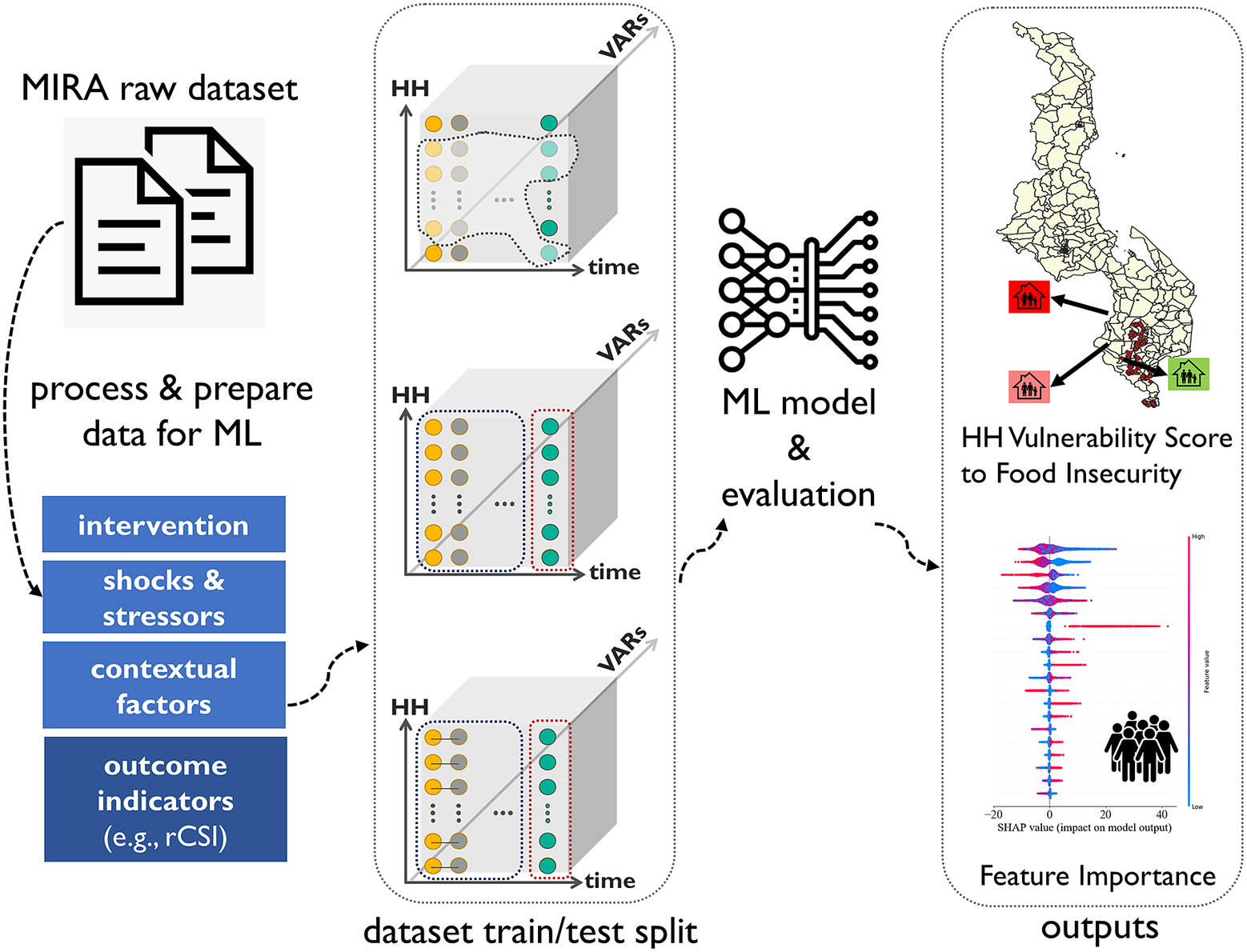
Figure 1. Machine learning workflow developed to study food security status of households and communities based on the Measurement Indicators for Resilience Analysis protocol.
The paper is structured as follows: Section 2 provides a brief overview of the literature on resilience measurement that guided the study. Section 3 provides the context for the HR data collection initiative, MIRA. Section 4 summarizes the data, including the use of the reduced Coping Strategy Index (rCSI) as a measure of food insecurity. Section 5 outlines the methodological validations, benchmarking the use of ML algorithms against a logistic regression (LR), shortlisting a series of predictors, and predicting future food security outcomes. Section 6 presents top predictors of food insecurity and the predictive performance of the model. Section 7 discusses the policy implications of these results. Section 8 concludes.
2. Literature Review
We contribute to a rapidly growing literature that focuses on using new, systematized approaches to improve predictions of food security. McBride et al. (Reference McBride, Barrett, Browne, Hu, Liu, Matteson, Sun and Wen2021) provide an excellent review of the existing evidence, emphasizing that these predictive models should be built for purpose.
Food security is a key welfare indicator, sensitive to seasonal and spatial variation. Estimates of the prevalence of food security are strongly correlated and depict similar trends over time, fluctuating between a relatively abundant period and a “hungry season,” often immediately preceding the harvest (Maxwell et al., Reference Maxwell, Vaitla and Coates2014). Many HHs oscillate in and out of food security throughout the year, a dynamic that is not necessarily captured by annual or bi-annual HH surveys (Anderson et al., Reference Anderson, Reynolds, Merfeld and Biscaye2018).
In terms of methodological improvements to predict welfare outcomes, McBride and Nichols (Reference McBride and Nichols2018) highlight the use of ML algorithms to improve the performance of the Proxy Means Testing. The authors argue that these algorithms should seek to optimize out-of-sample prediction by minimizing inclusion and exclusion errors. Kshirsagar et al. (Reference Kshirsagar, Wieczorek, Ramanathan and Wells2017) use LASSO to shortlist 10 variables that can be used for a predictive model of welfare, presenting a user-friendly approach that can be operationalized in the field.
In the context of predicting food security indicators, Cooper et al. (Reference Cooper, Brown, Hochrainer-Stigler, Pflug, McCallum, Fritz, Silva and Zvoleff2019) use geo-located data on child nutrition combined with localized climate and governance indicators to map where droughts have the largest effects on child stunting outcomes. Given the importance of data transparency and availability, Browne et al. (Reference Browne, Matteson, McBride, Hu, Liu, Sun, Wen and Barrett2021) show how a random forest (RF) model trained on open access data can predict contemporaneous and near-future food security outcomes in order to inform early warning systems. Andree et al. (Reference Andree, Chamorro, Kraay, Spencer and Wang2020) draw from historical IPCs, available at the subnational level, to predict future outcomes. Training the data on a series of geospatial and administrative indicators, the predictive algorithm outperforms the IPC own forecasts based on expert opinion. Their proposed model allows for a trade-off between inclusion and exclusion errors, reflecting policy preferences.
Maxwell et al. (Reference Maxwell, Caldwell and Langworthy2008) point out that a lack of HF food security data hinders early warning for food security crises. To improve these predictions, Headey and Barrett (Reference Headey and Barrett2015) emphasize the collection of HF monthly or quarterly data, as opposed to the standard survey administered on an annual or biannual basis. They recommend a panel design, like the one outlined by the Food Security Information Network, arguing that monitoring HHs over time would allow for the detailed examination of underlying determinants that improve HH resilience.
One of the earliest attempts to operationalize the use of HF panel data was by Mude et al. (Reference Mude, Barrett, McPeak, Kaitho and Kristjanson2009) to inform an early warning model in northern Kenya. Knippenberg et al. (Reference Knippenberg, Jensen and Constas2019) use HF HH food security data to demonstrate the cyclical and path dependent nature of HH food security. This predictive model allows them to create a shortlist of HH characteristics that impact HH food security outcomes. Lentz et al. (Reference Lentz, Michelson, Baylis and Zhou2019) use a log-linear model to predict food security outcomes in Malawi, using HH survey data combined with geospatial and price data. The additional resolution allows their predictive model to outperform IPC predictions.
3. Context: The MIRA Study
In the first few months of 2015, flooding in Malawi displaced an estimated 230,000 people, damaged about 64,000 hectares of land, and destroyed the asset wealth of many. By August 2015, the floodwaters receded and the majority of those displaced returned to their homes to rebuild their lives.
A consortium led by CRS was implementing the United in Building and Advancing Life Expectations (UBALE) program in three of the poorest and disaster-prone districts in Malawi – Chikwawa, Nsanje, and Rural Blantyre. UBALE was a 5-year, $63 million United States Agency for International Development (USAID)/FFP-funded Development Food Assistance Program being managed by CRS-Malawi. UBALE had a suite of overlapping interventions that aimed to sustainably reduce food insecurity and build resilience by reaching 250,000 vulnerable HHs in 284 communities. The main activities of the project included agriculture and livelihood, nutrition, and community disaster risk reduction activities, as well as a capacity strengthening component to strengthen and enhance existing systems and structures. The floods combined with the implementation of the UBALE program provided an excellent opportunity to examine HH resiliency and the factors that influence resilience.
The MIRA study officially started in May 2016 with a baseline evaluation and was then piloted over 3 months in the Chikwawa District. A full survey was developed to capture the initial states, capacities of HHs participating in the study, as well as shocks and stressors, and other HH characteristics, modeled on traditional HH surveys (see Table 12). This full survey was administered as a baseline, midline, and end line.
In addition, the researchers developed an HF questionnaire to be administered monthly. It was designed as a resilience-focused, low-burden tool, taking less than 10 min to administer. By collecting key indicators monthly, it provides essential information to track HH well-being trajectories over time in a shock-prone environment.
Following the pilot, the MIRA protocol was rolled out to 2,234 HHs across all three districts under the USAID-funded UBALE program. The selection of communities was randomized, stratified by access to the Shire river as the pilot had revealed this to be an important determinant of HH’s livelihood strategies. HHs within the community were selected at random from established registries which included all HHs in the community.Footnote 1 For this second cohort, over 37 rounds of data have been collected.
The MIRA protocol has been adopted by several other CRS country programs to collect more datasets. This ML study jointly conducted by CRS and Microsoft has led to the development of a scalable MIRA AI model in CRS, which is planned to be used as one packaged solution in other programs in CRS as well. In this paper, we focus our empirical analyses only on the Malawi dataset. However, once new datasets become available, the proposed ML workflow can be used on MIRA datasets from these other locations.
4. MIRA Dataset in Malawi: Case Study
To leverage the panel feature of the MIRA dataset for forecasting purposes, we selected the HHs that regularly participated in the MIRA program for at least 20 consecutive months from October 2017 to November 2019. This selection scheme resulted in 1,886 HHs for whom the data are included in our data science study described in the next sections. Table 1 outlines the difference in means across HHs that were retained and those that dropped off after the baseline. HHs that dropped out were slightly younger on average, had spent slightly less time in the village, and were more likely to rely on farming. With those caveats in mind, the retained sample remained broadly representative of the HHs in the community. Thus, in total, 37,720 observation records are available for our study. The visual distribution of the observations across southern Malawi is illustrated in Figure 2.Footnote 2
Table 1. Comparison of the sample of retained HHs versus HHs that dropped

Abbreviation: HH, household.

Figure 2. Malawi map and visual distribution of households.
All of the HHs are based in southern Malawi. When enumerators meet with HHs to conduct HF or annual surveys throughout the MIRA programs deployments, they keep records of HHs’ GPS locations and survey timestamps. Table 2 shows the geographical coverage of the MIRA dataset where TA and GVH denote Traditional Authorities and Group Village Headman. Table 3 shows some demographics information about these HHs.
Table 2. Measurement Indicators for Resilience Analysis coverage

Table 3. Basic HH demographics and livelihood information

Abbreviation: HH, household.
In this study, the outcome indicator for food security is the reduced coping strategy, rCSI, which is computed based on the coping strategy module questions outlined in Table 4. Our proposed models can be used for other food security metrics of interest, as well. To compute the rCSI score, we use equation (1), where $ s $
denotes a single coping strategy,
$ s $
denotes a single coping strategy, $ \mathcal{S} $
the set of coping strategies,
$ \mathcal{S} $
the set of coping strategies, $ {w}_s $
weights assigned to each strategy, and
$ {w}_s $
weights assigned to each strategy, and $ days $
the number of days each strategy is used by the HHs in the past 7 days. Weights are based on best practice in the literature (see Maxwell, Reference Maxwell1996) and are outlined in Table 4 for each strategy in the coping strategy index module:
$ days $
the number of days each strategy is used by the HHs in the past 7 days. Weights are based on best practice in the literature (see Maxwell, Reference Maxwell1996) and are outlined in Table 4 for each strategy in the coping strategy index module:
 $$ rCSI=\sum \limits_{s\in \mathcal{S}}\left({w}_s\cdotp {days}_s\right).\hskip0.5em $$
Table 4. Coping strategy index module in the Measurement Indicators for Resilience Analysis high-frequency survey and weights assigned to each strategy to compute rCSI score

Abbreviations: rCSI, reduced Coping Strategy Index.
Figure 3a demonstrates the histogram of the rCSI score for the entire dataset when all HHs and time steps are pooled together. Figure 3c,d shows the spatial distribution of rCSI scores across districts and TA areas in southern Malawi. Temporal distribution of the average raw rCSI score and a binary version of it, for two different thresholds of 16 and 19, are demonstrated in Figures 3b and 4a,b, respectively.

Figure 3. Reduced Coping Strategy Index score distributions.

Figure 4. Mean binary reduced Coping Strategy Index score distributions based on the two thresholds 19 and 16.
For further details of MIRA surveys, please see the snippets of the MIRA HF and annual survey modules shown in Tables 11 and 12.
5. Methodology
In this study, we pursue two goals: (Step I) conduct feature importance analysis to derive community-level insights on top predictors of food insecurity and (Step II) conduct food security forecasting to predict future food security outcomes. In this section, we present our ML approaches and methodologies for each of these goals.
Step I: Identifying key predictors
The first step is to calculate the top predictors of future food insecurity. To derive community-level insights from the MIRA dataset in Malawi, we use the entire dataset to train and test classical ML models. Then we select the top-performing model and apply a black-box interpretability technique, named Shapley additive explanations (SHAP; Lundberg and Lee, Reference Lundberg and Lee2017), to rank variables in terms of their contribution to the predicted outcomes. The SHAP framework uses game-theoretical notions to determine the contributions of predictor features to final predictions. This approach assumes that predictor features are similar to players in a coalitional game where the game payoff, which is the predicted probability in our problem, is distributed among the features based on Shapley concepts in game theory. In the game theory domain, the Shapley value is a solution concept of fairly distributing both gains and costs to several actors working in a coalition. SHAP can be applied to a variety of ML models as discussed in Lundberg and Lee (Reference Lundberg and Lee2017).
In this study, we focus on the rCSI score as the food security metric or the outcome indicator. We model the problem as a binary classification task where we convert the continuous outcome indicator into a binary variable, $ \mathbf{y}\in \left\{0,1\right\} $
, based on a threshold,
$ \mathbf{y}\in \left\{0,1\right\} $
, based on a threshold, $ \overline{r} CSI $
. Two cutoffs were used:
$ \overline{r} CSI $
. Two cutoffs were used: $ \overline{r} CSI=16 $
is the mean outcome in the dataset, splitting the sample into two halves.
$ \overline{r} CSI=16 $
is the mean outcome in the dataset, splitting the sample into two halves. $ \overline{r} CSI=19 $
represents a level of acute food insecurity that warrants provision of immediate humanitarian assistance.Footnote
3
$ \overline{r} CSI=19 $
represents a level of acute food insecurity that warrants provision of immediate humanitarian assistance.Footnote
3 $ y=1 $
represents the positive or food insecure, class and
$ y=1 $
represents the positive or food insecure, class and $ y=0 $
represents the negative or not food insecure class of HHs. We use all other HH variables collected as predictor or input features,
$ y=0 $
represents the negative or not food insecure class of HHs. We use all other HH variables collected as predictor or input features, $ {x}_i $
, to predict the outcome indicator,
$ {x}_i $
, to predict the outcome indicator, $ {y}_i $
.
$ {y}_i $
.
To train a predictive model, we use LR and RF approaches. The LR models the posterior probabilities of the classes via a linear function in input features, that is, $ {x}_i $
, while at the same time ensuring that they sum to one and remain in
$ {x}_i $
, while at the same time ensuring that they sum to one and remain in $ \left[0,1\right] $
. In contrast to the logistic model, regression trees can capture complex interactions between features. Tree-based methods partition the feature space into a set of rectangles and then fit a simple model (e.g., a constant) in each one. However, trees are noisy and suffer from high variance. To improve the variance reduction, the RF is a reasonable choice as they are built based on a large collection of de-correlated trees and averaging their results. More details about these classical ML models can be found in Friedman et al. (Reference Friedman, Hastie and Tibshirani2001).
$ \left[0,1\right] $
. In contrast to the logistic model, regression trees can capture complex interactions between features. Tree-based methods partition the feature space into a set of rectangles and then fit a simple model (e.g., a constant) in each one. However, trees are noisy and suffer from high variance. To improve the variance reduction, the RF is a reasonable choice as they are built based on a large collection of de-correlated trees and averaging their results. More details about these classical ML models can be found in Friedman et al. (Reference Friedman, Hastie and Tibshirani2001).
Dataset preparation for ML is demonstrated visually in Figure 5a for more clarity. In Figure 5a, we focus on one HH for demonstration; thus, we skip the vertical axis that indicates all HHs. The horizontal axis denotes time steps, and the depth axis denotes all available variables including predictor features (i.e., information captured in shock, assistance, and contextual data modules in MIRA surveys that might influence the food security status of the HHs) and the outcome indicator (i.e., the rCSI score for which we aim to make predictions). Each variable is demonstrated by a circle. Each arrow that is drawn on a row of circles denotes one data point for which predictor features are associated with the rCSI score in the corresponding time step.

Figure 5. Machine learning dataset preparation and split scheme with cross-sectional data assumption where independent variables are used as predictor features for the reduced Coping Strategy Index score at the time step. Records are pooled together for HHs and time steps to generate a randomized data split. The horizontal axis denotes time, the vertical axis denotes HHs, and the depth axis denotes independent variables.
Note that although this data preparation approach provides insights about the population, this scheme for data point generation cannot be used for forecasting purposes since predictor features and the outcome indicator come from the same time step for each data point. Moreover, the explicit temporal aspect of the dataset is not modeled for this analysis. Rather, we include the monthly information as one of the predictor features and rely on inherent and implicit temporal information in the dataset. We change these assumptions, in our second approach described in the next section, where we propose a forecasting model at the HH level.
We denote the dataset as $ \mathcal{D}=\left(\mathbf{X},\mathbf{y}\right) $
where
$ \mathcal{D}=\left(\mathbf{X},\mathbf{y}\right) $
where $ \mathbf{X}\in {\mathrm{\mathbb{R}}}^{TN\times f} $
is a matrix of
$ \mathbf{X}\in {\mathrm{\mathbb{R}}}^{TN\times f} $
is a matrix of $ f $
predictor features recorded at each of these
$ f $
predictor features recorded at each of these $ T $
discrete time steps and
$ T $
discrete time steps and $ N $
HHs. Each time step
$ N $
HHs. Each time step $ t\in \left[T\right] $
is 1-month long, and each location
$ t\in \left[T\right] $
is 1-month long, and each location $ n\in \left[N\right] $
denotes an HH that has participated and is included in our study.
$ n\in \left[N\right] $
denotes an HH that has participated and is included in our study. $ \mathbf{y}\in {\left\{0,1\right\}}^{TN} $
denotes the observation vector associated with all data points. Finally, we pool together the entire data points for all HHs across all time steps and split into train/test portions randomly for ML modeling as illustrated in Figure 5b.
$ \mathbf{y}\in {\left\{0,1\right\}}^{TN} $
denotes the observation vector associated with all data points. Finally, we pool together the entire data points for all HHs across all time steps and split into train/test portions randomly for ML modeling as illustrated in Figure 5b.
Step II: Predicting future food insecurity
Having identified key predictors using a cross-sectional approach, to derive HH-level insights, we propose to leverage the ML framework and time-series characteristics of the MIRA dataset. The goal is to forecast the vulnerability of each HH to food insecurity based on their historical records. To that end, we use the neural network (NN) architectures proposed in Wang et al. (Reference Wang, Yan and Oates2017) along with the RF model to compare their performances in similar settings.
Figure 6 can be used as a visual demonstrator of the dataset preparation scheme. Each variable at each time step is demonstrated by a circle. Figure 6a shows all the variables for one HH. Thus, we skipped the vertical axis that indicates all HHs. The horizontal axis denotes time steps, and the depth axis denotes all variables including predictor features (i.e., information captured in shock, assistance, and contextual data modules in MIRA surveys that might influence HHs food security) and the outcome indicator (i.e., the rCSI score for which we aim to make predictions).

Figure 6. Time-series data point preparation and split scheme. The horizontal axis denotes time, the vertical axis denotes households, and the depth axis denotes independent variables.
We now allow a time window for predictor features to be used in the ML model. For example, in Figure 6a, each parallelogram shows the variables and their time window used to predict the outcome indicator. The parallelogram is connected to the corresponding outcome variable via an arrow. Depending on the selected time window for the time series and the entire time covered by the dataset, we slide the parallelogram to generate more data points for each HH. When identifying predictors, we used predictor features and the outcome indicator from the same time step $ t $
; here, the outcome variable, food insecurity, comes from the next time step
$ t $
; here, the outcome variable, food insecurity, comes from the next time step $ t+1 $
to ensure that the analysis is suitable for forecasting. Once all the data points are generated, we split the data into train/test sets considering time order. In other words, we use the data of all HHs from the very last time step as the test set and all other data points before the last time step as the training set.
$ t+1 $
to ensure that the analysis is suitable for forecasting. Once all the data points are generated, we split the data into train/test sets considering time order. In other words, we use the data of all HHs from the very last time step as the test set and all other data points before the last time step as the training set.
Figure 7 demonstrates the details of the layers for all NN models. Figure 7a shows the details of the multilayer perceptron (MLP) model, which contains three hidden layers consisting of 500 fully connected neurons. Each of the hidden layers is followed by a ReLU activation function to add nonlinearity to the model. ReLU stands for rectified linear activation function, which is a piecewise linear function that outputs the input directly if it is positive; otherwise, it outputs zero, if the input is negative. The final layer is a softmax function to convert the output of the network to the values between $ 0 $
and
$ 0 $
and $ 1 $
. A softmax function is a generalization of the logistic function to multiple dimensions to normalize the output of a network to a probability distribution over predicted output classes. The dashed lines in the plot show the dropout rate, which denotes the regularization method used to avoid overfitting during the training. Figure 7b shows the convolutional neural network (CNN). The main building blocks in CNNs are convolutional layers, which are the basic process of applying a filter to an input to produce an output activation. This operation has been shown to be effective in fields like computer vision in extracting unique features. The network used in this study consists of two convolutional layers with 6 and 12 filters followed by a sigmoid function to add nonlinearity to the network. The final layer is a softmax layer to convert outputs properly for the binary classification task. Figure 7c demonstrates the Resnet architecture in which some skip connections are introduced and ReLU activation is used to add nonlinearity. Furthermore, batch normalization operations are considered to make artificial NNs faster and more stable through the normalization of the input layer by re-centering and re-scaling. This model also contains a pooling layer that reduces the spatial size of the representation to reduce the number of parameters and computation in the network. The final layer is a softmax function.
$ 1 $
. A softmax function is a generalization of the logistic function to multiple dimensions to normalize the output of a network to a probability distribution over predicted output classes. The dashed lines in the plot show the dropout rate, which denotes the regularization method used to avoid overfitting during the training. Figure 7b shows the convolutional neural network (CNN). The main building blocks in CNNs are convolutional layers, which are the basic process of applying a filter to an input to produce an output activation. This operation has been shown to be effective in fields like computer vision in extracting unique features. The network used in this study consists of two convolutional layers with 6 and 12 filters followed by a sigmoid function to add nonlinearity to the network. The final layer is a softmax layer to convert outputs properly for the binary classification task. Figure 7c demonstrates the Resnet architecture in which some skip connections are introduced and ReLU activation is used to add nonlinearity. Furthermore, batch normalization operations are considered to make artificial NNs faster and more stable through the normalization of the input layer by re-centering and re-scaling. This model also contains a pooling layer that reduces the spatial size of the representation to reduce the number of parameters and computation in the network. The final layer is a softmax function.

Figure 7. Neural Nets used for time-series forecasting.
6. Results
In this study, we aim to present a proof of concept to use ML predictive modeling and interpretability frameworks in food security domain to develop insights for stakeholders. We evaluate several data modeling scenarios and report validation results to reflect on the models’ performance and robustness. To quantitatively evaluate the performance of trained ML models, we use standard metrics including precision, recall, F1, and accuracy defined in Table 5. For some of our experiments in this study, we only focus on F1 score, an aggregate metric that reflects simultaneously on both precision and recall metrics. It is computed as the harmonic mean of precision and recall, for which the equation is shown in Table 5.
Table 5. Evaluation metrics for performance of classifier

Abbreviation: HH, household.
Step I results: Key predictors
In this section, we demonstrate the results of SHAP framework on top of RF predictive model. We also evaluate performance of both RF model and the LR model as the baseline for comparison. After data processing, 37,720 records and 126 predictor variables are available for our experiments. Due to space consideration, we only show a selected list of variables in Table 3 and in the survey snippets in Tables 11 and 12. We have converted all the variables into monthly data. For the annual surveys, we assumed those variables remained similar across different months in a specific year. These variables have been collected annually since they are not expected to change at a fast pace. In this experiment, we apply fivefold cross-validation and random shuffling on the dataset (Table 6). For each fold, an LR model and an RF model are trained on 75% of the Malawi dataset and assessed on the unseen 25% of the data. We split the dataset in a randomized way to create each fold. For the binarization of the rCSI score based on the threshold 16, the class imbalance (ratio of positive to negative classes) in the dataset is 47.81% for the training set and 48.81% for the test set. For the threshold 19, these numbers are 39.01 and 40.52%. We report the average performance across all folds.
Table 6. Comparing classical ML model performances based on random partitioning of the dataset

Abbreviations: LR, logistic regression; ML, machine learning; RF, random forest.
The evaluation results for ML models performance are shown in Table 7 using LR and RF. The cutoff threshold indicates the threshold values, $ \overline{r} CSI $
, above which HHs are classified as food insecure, converting the rCSI score to a binary variable. The RF model outperforms the LR across metrics and for both threshold values. We then apply the SHAP framework to tease out the most predictive variables that inform future food insecurity.
$ \overline{r} CSI $
, above which HHs are classified as food insecure, converting the rCSI score to a binary variable. The RF model outperforms the LR across metrics and for both threshold values. We then apply the SHAP framework to tease out the most predictive variables that inform future food insecurity.
Table 7. Predictive performance using previous rCSI + SHAP top 20 features and 15 months of data

Abbreviations: CNN, convolutional neural network; MLP, multilayer perceptron; rCSI, reduced Coping Strategy Index; RF, random forest; SHAP, Shapley additive explanations.
In Figure 8a, we see the global summary results of the SHAP analysis. The SHAP value, shown on the x-axis, indicates the contribution of each specific feature to the model output for each data point. The larger SHAP values correspond to larger contribution of the specific feature to the model outputs, which are the predicted probability for vulnerability to food insecurity. Positive SHAP values correspond to positive contribution to the predicted probabilities, and negative values indicate negative contribution to probability predicted by the model. The relative value of each feature is shown with colors on the dots where blue indicates small and red indicates large values. The features are demonstrated on the y-axis where they are ordered globally based on their average level of contributions to the final predictions, according to the corresponding SHAP values for the entire dataset, collectively. In this plot, overlapping points are jittered in the y-axis direction to get a sense of the distribution of the Shapley values per feature. We used the InterpretML 0.2.7 Python library for the SHAP implementation and generation of summary and dependence plots. As shown in the plot, the locations of the HHs are among the top features and have contributed significantly to the final predictions, and thus they have resulted in a wider range of SHAP values. This reflects how food insecurity is a co-variate phenomenon, concentrated in specific areas where HHs are disproportionately poor and lack access to safety nets. Moreover, this observation indicates that the models are location-specific, and thus they should be retrained for each new site.

Figure 8. Shapley additive explanations global and dependence plots.
Future welfare and overall status are also among the top predictor features. To analyze these variables further, we also show SHAP dependence plots. Figures 8c,d demonstrates that an increase in self-evaluation of future welfare and overall status corresponds to a downward trend in SHAP values and the corresponding vulnerability scores. The colors shown in the dependence plots indicate a second feature, chosen automatically by the SHAP algorithm, that may have an interaction effect with the feature we are plotting. If an interaction effect is present between this other feature and the feature we are plotting, it will show up as a distinct vertical pattern of coloring. For the three variables shown in Figure 8, we do not observe such meaningful interaction effects. The SHAP dependence plot for time variable is shown in Figure 8b, where upward trends visible from October to February align with the patterns observed in Figures 3b and 4a,b.
Step II results: Predicting future outcomes
To evaluate the performance of respective models, we report the F1 score. As before, the outcome indicator is a binary variable using the threshold $ \overline{r} CSI $
. In the plots shown in Figures 9 and 10, the y-axis indicates the F1 score and the x-axis indicates time-series length used to prepare the dataset. In each plot, there are five curves for the cases where (a) only the past rCSI score, (b) the rCSI score along with the SHAP top 8 features from Step 1, (c) the rCSI score along with the SHAP top 20 features, (d) only the SHAP top 8 features, or (e) only the SHAP top 20 features are used as the predictor features subset in ML models. We transform the MIRA dataset into three-dimensional arrays where the first dimension represents a record or data point generated based on the sliding window scheme shown in Figure 6. Depending on the length of the time series used and the number of variables included in the experiment, the training and test set sizes vary. For example, for case (c), the training set size is (13,202, 21, 12) and the test set size is (1,886, 21, 12), where the first, second, and third dimensions show the number of records, number of variables, and length of the time series used, respectively. Note that in case (c), variables used include historical rCSI scores along with the SHAP selected 20 variables. For the MLP and RF models, this multidimensional input array needs to be reshaped into (13,202, 252) and (1,886, 252), where the second dimensions represent the number of time steps and variables used in an aggregate way. In this case, for the threshold 19, the positive class represents 33.71 and 36.85% of the datasets, in the training set and the test set, respectively. For the threshold 16, these numbers are 42.59 and 45.28%. We kept 10% of the training data for validation. The test set is created based on the data from the last time step in November 2019. In the next section, we show the model’s robustness across multiple future time steps.
$ \overline{r} CSI $
. In the plots shown in Figures 9 and 10, the y-axis indicates the F1 score and the x-axis indicates time-series length used to prepare the dataset. In each plot, there are five curves for the cases where (a) only the past rCSI score, (b) the rCSI score along with the SHAP top 8 features from Step 1, (c) the rCSI score along with the SHAP top 20 features, (d) only the SHAP top 8 features, or (e) only the SHAP top 20 features are used as the predictor features subset in ML models. We transform the MIRA dataset into three-dimensional arrays where the first dimension represents a record or data point generated based on the sliding window scheme shown in Figure 6. Depending on the length of the time series used and the number of variables included in the experiment, the training and test set sizes vary. For example, for case (c), the training set size is (13,202, 21, 12) and the test set size is (1,886, 21, 12), where the first, second, and third dimensions show the number of records, number of variables, and length of the time series used, respectively. Note that in case (c), variables used include historical rCSI scores along with the SHAP selected 20 variables. For the MLP and RF models, this multidimensional input array needs to be reshaped into (13,202, 252) and (1,886, 252), where the second dimensions represent the number of time steps and variables used in an aggregate way. In this case, for the threshold 19, the positive class represents 33.71 and 36.85% of the datasets, in the training set and the test set, respectively. For the threshold 16, these numbers are 42.59 and 45.28%. We kept 10% of the training data for validation. The test set is created based on the data from the last time step in November 2019. In the next section, we show the model’s robustness across multiple future time steps.

Figure 9. Evaluation results versus time-series length (reduced Coping Strategy Index cutoff = 19).

Figure 10. Evaluation results versus time-series length (reduced Coping Strategy Index cutoff = 16).
For NN models, excluding rCSI score as time series, as shown in cases (d) and (e), deteriorates performance significantly. Across configurations, case (c) is consistently among the top-performing models. Most of the presented models demonstrate decent performance with at least 15 months of data. This amount of data would capture all seasonal fluctuations. Time-series length also had a significant impact on Resnet results.
All other metrics are summarized for the optimal setup, that is, using rCSI + SHAP top 20 features and time-series length of 15 months, in Table 7.
Robustness: Additional time steps
Even if model parameters can be updated in real time based on the most up-to-date data collected from the field, there is value in forecasting several months into the future to inform the planned delivery of assistance. To that end, we demonstrate the performance of our proposed approach up to 4 months in the future in Table 8. Since the length of time series impacts the number of time steps available for training and testing, we use a semi-optimal configuration with a 12-month predictive window where each HH has eight rounds of outcomes. This allows reasonable number of time steps available for training and testing. We train our model on the first four time steps and leave the last four time steps for validation. Since we are assigning more data to the validation set and fewer data to the training set, performance deteriorates slightly, but 4 months out the model can still predict food insecure HHs with an F1 between 0.664 and 0.735 and an accuracy between 0.792 and 0.784.
Table 8. RF model performance across multiple steps ahead using rCSI + SHAP top 20 features and length of 12 months for time series

Abbreviations: rCSI, reduced Coping Strategy Index; RF, random forest; SHAP, Shapley additive explanations.
Tables 9 and 10 show confusion matrix for all time steps and both thresholds to demonstrate Type-I (false-positive) and Type-II (false-negative) errors. For the threshold $ \overline{C} SI=19 $
, the predictions show a consistent false negative of 11% and a false positive of 30–35%. Lowering the threshold to
$ \overline{C} SI=19 $
, the predictions show a consistent false negative of 11% and a false positive of 30–35%. Lowering the threshold to $ \overline{C} SI=16 $
decreases the false negative rate to 7%, but increases the false positive rate to between 34 and 45%. The false negatives are stable across time steps, whereas the false positives increase. Were these predictions tied to the disbursement of assistance, these different thresholds highlight the trade-off between exclusion error, where eligible HHs would not receive assistance, and inclusion error, where noneligible HHs would receive assistance.
$ \overline{C} SI=16 $
decreases the false negative rate to 7%, but increases the false positive rate to between 34 and 45%. The false negatives are stable across time steps, whereas the false positives increase. Were these predictions tied to the disbursement of assistance, these different thresholds highlight the trade-off between exclusion error, where eligible HHs would not receive assistance, and inclusion error, where noneligible HHs would receive assistance.
Table 9. Confusion matrix for the threshold 19 and random forest results for robustness check presented in Table 8

Abbreviation: ts, time step.
Table 10. Confusion matrix for the threshold 16 and random forest results for robustness check presented in Table 8

Abbreviation: ts, time step.
7. Policy Implications
These results provide a use case in how to leverage ML algorithms trained on HF data to predict future levels of food insecurity.
The analysis allows us to shortlist which features have the greatest predictive power and should accordingly be monitored. Previous food security as measured using rCSI is an informative feature, indicating its persistence within HHs over time. Through the SHAP framework, we can infer that other highly predictive features are location, current, and future subjective notions of welfare, seasonal information, experienced shocks, and social assistance. While these should not be interpreted causally, these results highlight that for the regions studied here, a small subset of 21 indicators out 126 accounts for most of the variation in food insecurity. Monitoring these features can be done rapidly and at a low cost. Location and prices can be monitored remotely, while other indicators can be solicited either through in-person interviews or over the phone. Since rCSI is composed of five indicators, it could even be collected cost effectively via short message service or interactive voice response.
The analysis also demonstrates the value added from collecting HF data that capture seasonal fluctuations. Once 1 year of observations is included in the algorithm, the predictive power as measured using the F1 metric increases significantly. This algorithm can predict outcomes up to 4 months in the future, providing sufficient time for government agencies and humanitarians to mobilize and distribute assistance. Unlike other ML efforts that focus on large administrative areas, this can be targeted at the community level, and even down to HHs if necessary, based on their previous history of food insecurity.
Finally, this paper demonstrates a use case driven by imperatives on the ground, and one that is being scaled up at the national level. By proving both cost effective and policy-relevant, the MIRA methodological approach has gained many adherents. It is being implemented in additional countries, including Madagascar and Ethiopia. The World Bank, USAID, and Department for International Development have all financed HF monitoring systems in Malawi relying on sentinel sites, drawing from the MIRA protocol. To ensure that these efforts are integrated into national institutions, CRS and its partners are currently engaged with the government of Malawi to incorporate MIRA into its national resilience strategy.
8. Conclusion
In this study, we demonstrated how ML modeling combined with HF sentinel data can be leveraged to predict future food insecurity. Twenty-one key predictors are sufficient to predict community and HH food security outcomes up to 4 months into the future. Highlighting the importance of seasonality, including at least 15 months of historical data boosts model performance significantly.
While our empirical analysis is based on HF MIRA survey data collected in southern Malawi, our proposed methodology can be applied to other HF datasets. In particular, this paper serves as one more exemplar of the value of embedded HF sentinel sites to monitor food security. Once in place and combined with sophisticated algorithms, these can predict food security outcomes and present actionable knowledge about low-resource communities for stakeholders and authorities. Such knowledge can inform more targeted intervention programs.
Funding Statement
This research was supported by grants from the Microsoft AI for Humanitarian Actions Program.
Competing Interests
The authors declare no competing interests exist.
Author Contributions
J.C. and E.K. designed the on-site data collection program and led the data cleaning process. J.C. wrote the context section. S.G. designed the ML workflow, conducted the empirical analysis, and wrote the ML technical sections and results. E.K. informed the data analysis, and wrote the introduction, literature review, and data and policy implication sections. D.A. and A.K. enabled planning for internal operationalization of the ML workflow at CRS. A.K., P.P., and R.S. conducted program management efforts for this collaborative project jointly done by CRS and Microsoft. C.B. and J.L.F. reviewed and approved the final version of the manuscript.
Data Availability Statement
Dataset is not publicly available.
9. Annex
Table 11. MIRA high-frequency survey snippet.

Table 12. MIRA annual survey snippet.


 Open access
Comments
No Comments have been published for this article.