


Notation
 $\Omega$
a subspace of the usual 3D Euclidian space.
- $\textbf{x}$
a 3D point where
$\textbf{x} \in \Omega$.- t
the usual time variable.
- $\textbf{o}(\textbf{x})$
the occupancy field.
- K or $K_j$
a 3D spatial cell such that
$\Omega = \cup_{j=1}^N K_j$.- $\textbf{o}_K$ and $\bar{\textbf{o}}_K$
occupied and unoccupied states in cell K.
- $s_K$
distance traversed by a lidar ray in cell K.
- $n_K$
number of reflected rays in cell K.
- $\textbf{r}$
denotes the direction of a lidar ray in 3D.
- $\mathfrak{D}$
data space.
- $\mathfrak{M}$
model space.
- $\textbf{d}$
an outcome of the sample space associated to
$\mathfrak{D}$.- $\textbf{m}$
an outcome of the sample space associated to
$\mathfrak{M}$.- $\textbf{D}$
measured outcome on
$\mathfrak{D}$. Note that $\textbf{D}$ represents a measurement as opposed to $\textbf{d}$ which represents a variable.- $\mu_{\mathrm{D}}$ and $\mu_{\mathrm{M}}$
homogeneous measures on data and model spaces.
- $\varphi_\mathrm{D}$ and $\varphi_\mathrm{M}$
measurable functions on data and model spaces, respectively.
- $\tilde{\mathfrak{D}}$
codomain of
$\varphi_\mathrm{D}$, that is new data space.- $\tilde{\mathfrak{M}}$
codomain of
$\varphi_\mathrm{M}$, that is new model space.- $\tilde{\textbf{d}}$
an outcome of the sample space associated to
$\tilde{\mathfrak{D}}$.- $\tilde{\textbf{m}}$
an outcome of the sample space associated to
$\tilde{\mathfrak{M}}$.- $\mu_{\tilde{\mathrm{D}}}$ and $\mu_{\tilde{\mathrm{M}}}$
homogeneous measures on new data and new model spaces.
- c
speed of light.
- $\{t_i\}_{i \in I}$
first arrivals detected by the lidar instrument.
- $\textbf{x}_0$
lidar location in 3D.


Note: subscript K (e.g.,  $\tilde{\textbf{m}}_K$) denotes a constant field value associated to cell K. Throughout the manuscipt, we use
  $d\mu_{\mathrm{M}}$ in place of
  $d\mu_{\mathrm{M}}(\textbf{m})$ to shorten the length of equations.
1. Introduction
Lidar sensors are accurate, reliable, and highly popular sensors in mobile robotics. Current data assimilation algorithms for onboard sensors mostly focus toward decreasing computation time and improving localization accuracy for Simultaneous Localization And Mapping (SLAM). As a result, a significant fraction of these algorithms pay little attention to map parameters and mainly operate in the data space [Reference Pire, Baravalle, D’alessandro and Civera1,Reference Shan and Englot2]. For instance, in Lidar Odometry And Mapping (LOAM), lidar data are represented as point clouds and robot relative location is achieved by directly matching edge and planar features extracted from point clouds [Reference Zhang and Singh3]. Recent advances in machine learning algorithms have further accelerated this trend [Reference Ramezani, Tinchev, Iuganov and Fallon4,Reference Tinchev, Penate-Sanchez and Fallon5]. While relative localization and computation efficiency are essential when dealing with mobile platforms, quantitative assessment of map parameters can also be valuable. In particular, explicitly using material parameters requires a well-defined forward model embedding the physics at hand. An explicit link to the underlying physics can be useful to assess relative robustness of algorithms by comparing material parameters used in each algorithm. Mapping material parameters can also be a precious source of information for autonomous agents operating in unknown complex environments [Reference Rekleitis, Bedwani and Dupuis6,Reference Opromolla, Fasano, Rufino, Grassi and Savvaris7] or performing scientific tasks [Reference Lee, Kommedal, Horchler, Amoroso, Snyder and Birgisson8,Reference Ceccarelli, Cafolla, Carbone, Russo, Cigola, Senatore, Gallozzi, Di Maccio, Ferrante, Bolici, Supino, Colella, Bianchi, Intrisano, Recinto, Micheli, Vistocco, Nuccio and Porcelli9]. The early work of Elfes [Reference Elfes10] has been a the forefront of map parameter estimation using lidar Bayesian data assimilation for occupancy mapping [Reference Chen, Chen, Zhu, Su, Zhou, Guan and Liu11–Reference Burgard, Fox, Hennig and Schmidt13]. Unfortunately, occupancy mapping algorithms suffer from multiple shortcomings, which find their roots in the lack of physical definition of the occupancy state. The absence of a clear definition of the occupied state of a cell when using occupancy grid mapping is a good example of such shortcomings. Indeed, how much occupied a cell needs to be in order to be defined as occupied? Can we define the degree of occupancy of a cell? How does the occupancy state relate to physical quantities such as dielectric permittivity, reflectivity, mean free path? These limitations eventually hamper quantitative estimations of map quality. Interestingly, attempts to overcome occupancy mapping limitations can be found in the literature. In Thrun’s study [Reference Thrun12], the problem is presented as trying to recover the local probability of reflection in place of occupancy. Alternatively, Deschaud et al. [Reference Deschaud, Prasser, Dias, Browning and Rander14] introduce a permeability field parameter to account for random data generation. Levinson and Thrun [Reference Levinson and Thrun15] achieve a substantial improvement through the use of probabilistic infrared reflectivity parameters taking into account measured reflected intensities. In spite of these attempts, we believe there remains a need for a sound mathematical treatment of quantitative data assimilation with physics related map parameters.
In data assimilation, the forward model can be understood as a relation between recorded data and model parameters. Practically, forward models often account for the physics at hand. For instance, Maxwell’s equations along with constitutive relations allow in theory to relate measured lidar data to dielectric permittivity and permeability fields. In such a case, dielectric permittivity and permeability fields correspond to model parameters while Maxwell’s equations and constitutive relations act as the forward model. This forward model can be labeled as deterministic since, for given dielectric permittivity and permeability fields, if our lidar instrument is perfect, recorded lidar values are fully known. In practice, using these model parameters and forward model for lidar data assimilation would be unrealistic, especially when dealing with onboard real-time computation. Thankfully, it is possible to use coarser model parameters associated to nondeterministic (or probabilistic) forward models, which are much less expensive to compute. These model parameters, along with their probabilistic forward models, allow to recover quantitative information on the environment from lidar recordings. In this paper, we propose to use the underlying physics to derive such model parameters and their associated probabilistic forward models. In particular, we show how these model parameters relate to lidar mean free path and to the concept of local degree of occupancy. Using these new model parameters and forward models, we introduce a new lidar data assimilation algorithm, which can be used for onboard real-time mapping. Main advantages of the proposed algorithm lie in its ability to relate model parameters to physics which, is of paramount importance for quantitative information retrieval, comparison of data assimilation algorithms, and data fusion.
The paper is divided into three distinct sections. The first section discusses main shortcomings of classic occupancy grid mapping algorithms. This section illustrates the motivations for this work. The second section details the underlying mathematical framework, which allows to reconciliate Bayes’ inference rule and probabilistic forward models with the underlying physics. It offers a clear insight on how to relate physics to our model parameters in theory. The last section applies results from the third section to lidar mapping for mobile robots. It introduces a new forward model with new model parameters for onboard lidar data assimilation. A careful and detailed analysis is provided to understand how our new approach relates to classic occupancy mapping. An example is further provided to illustrate our results.
2. Overview of Occupancy Grid Mapping
The well-established occupancy grid formalism seeks to assimilate lidar data to deliver a real-time occupancy map of the environment (see Fig. 1). Basic sensor lidar data assimilation algorithm using the occupancy grid framework can be derived from Bayes’ rule [Reference Elfes10,Reference Thrun12,Reference Thrun, Burgard and Fox16]. We introduce the forward model, also known as the sampling distribution, which is simply described by  $p(\textbf{d} | \textbf{o} )$ [Reference Jaynes17,18]. It corresponds to the probability to record
  $\textbf{d}$ from a single lidar ray given an occupancy field
  $\textbf{o}$. The occupancy field is a binary field which, in this framework, lives on a 3D grid. Accordingly, we let
  $\textbf{o}_K$ be the occupied state in cell K and
  $\bar{\textbf{o}}_K$ be to the unoccupied state. Using Bayes’ rule, the elementary occupancy parameter estimation equation can be derived as
 \begin{equation}\begin{aligned}p(\textbf{o}| \textbf{d} ) = \frac{p(\textbf{o}) \, p(\textbf{d} | \textbf{o})}{\int_{\mathfrak{O}} p(\textbf{o}) \, p(\textbf{d} | \textbf{o}) \, d\textbf{o}}\end{aligned}\end{equation}
 where  $\mathfrak{O}$ is to the set of all possible occupancy fields and
  $p(\textbf{o})$ represents our prior information on the occupancy field.
  $p(\textbf{o}| \textbf{d} )$ thus corresponds to the well-known inverse sensor model [Reference Thrun, Burgard and Fox16]. At this point, all we need is to specify the forward model
  $p( \textbf{d} | \textbf{o} )$.

Figure 1. Schematic configuration of lidar data acquisition using a mobile robot. Red dotted lines represent lidar rays. The robot record time of flight is associated to each ray. Several voxels associated to the occupancy field discretization for mapping purpose are displayed in blue. Rover image credit: NASA/JPL–Caltech
2.1. Defining the occupancy state
Attempts at proper mapping and localization over the years have yielded numerous alternative expressions for the forward model. Surprisingly, in many occupancy algorithms, it is common not to explicitly provide a physical definition of the occupancy state [Reference Thrun, Burgard and Fox16]. As a result, the occupancy is implicitly defined through its associated forward model  $p(\textbf{d} | \textbf{o} )$. However, in practice, forward models are usually derived using real-world parameters in place of the occupancy model parameter. The lack of clear connection between forward models and the occupancy field results in a loose definition of the occupancy parameter. Note that this issue is further discussed in Section 3.3. A more formal way to inspect this definition issue is to study the occupancy state of a cell a posteriori. A cell K is naturally defined as occupied if its posterior probability value
  $p(\textbf{o}_K| \{\textbf{D}_i\}_{i \in I} )$ converges toward 1 as the number of (relevant and accurate) measurements N converges toward infinity. A cell K is unoccupied if its posterior probability value converges toward 0. We introduce the true intrinsic probability
  $\alpha(\textbf{d}|W)$, which is the probability to generate a single lidar measurement
  $\textbf{d}$ given the real world W during our experiment. This intrinsic probability is neither
  $p(\textbf{d}|\bar{\textbf{o}}_K )$ or
  $p(\textbf{d}|\textbf{o}_K )$, but corresponds to the statistical response induced by the true physical parameters that affects our measurements. We let the data space be
  $\mathfrak{D}$ such that
  $\textbf{d} \in \mathfrak{D}$ and
  $\textbf{D}_i \in \mathfrak{D}$ for all i. Then, for each cell K, we can write (see Appendix A for details),
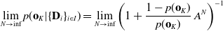 \begin{equation}\begin{aligned}\lim_{N \to \inf} p(\textbf{o}_K| \{\textbf{D}_i\}_{i \in I} ) = \lim_{N \to \inf} \left( 1 + \frac{ 1- p(\textbf{o}_K) }{p(\textbf{o}_K)} \, A ^N \right)^{-1}\end{aligned}\end{equation}
where
 \begin{equation}\begin{aligned}A = \exp \left( \int_{\mathfrak{D}} \alpha(\textbf{d}|W) \, \log\frac{ p( \textbf{d} | \bar{\textbf{o}}_K ) }{p( \textbf{d}| \textbf{o}_K )} \, d \mu_{\mathrm{D}} \right)\end{aligned}\end{equation}
 As N converges toward infinity,  $p(\textbf{o}_K| \{\textbf{D}_i\}_{i \in I} )$ converges to 1 if
  $A<1$, it converges to
  $p(\textbf{o}_K)$ if
  $A=1$ and to 0 if
  $A>1$. Thus, the previous equation provides an explicit definition of the occupancy state in cell K given the cell lidar response. In other words, cell K is occupied if its lidar response
  $\alpha(\textbf{d}|W)$ is such that
  $A<1$. It is possible to show, using Gibbs’ inequality, which
  $\alpha(\textbf{d}|W)=p( \textbf{d} | \textbf{o}_K )$ results in
  $A \leq 1$ and
  $\alpha(\textbf{d}|W)=p( \textbf{d} | \bar{\textbf{o}}_K )$ results in
  $A \geq 1$. However, this definition is impractical and remains highly abstract.
2.2. Occupancy inverse models versus forward models
Occupancy grid algorithms can further suffer from issues related to the underlying prior used. We discuss here the occupancy grid algorithm Octomap introduced by Hornung et al. [Reference Hornung, Wurm, Bennewitz, Stachniss and Burgard19], which is widely used in the mobile robotics community. Octomap relies on an elementary forward model, where  $p(\textbf{d}|\textbf{o} )$ is fully determined by
  $\cup_K \{p( \textbf{d}|\textbf{o}_K ),p( \textbf{d}|\bar{\textbf{o}}_K )\}$ and where measurements are usually assumed independent. As a result,
  $p(\textbf{d} | \textbf{o}_K )$ and
  $p(\textbf{d} | \bar{\textbf{o}}_K )$, which correspond to the probabilities that a single lidar ray measures
  $\textbf{d}$ if the cell K state is occupied or unoccupied, respectively, are sufficient to describe the full forward model. The occupancy state is thus fully determined by both values
  $p( \textbf{d} | \textbf{o}_K )$ and
  $p( \textbf{d} | \bar{\textbf{o}}_K )$. If we let
  $\mathscr{K}_e$ be the set of all unoccupied cells and
  $\mathscr{K}_f$ be the set of all occupied cells, we can explicitly write the resulting occupancy grid forward model,
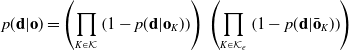 \begin{equation}\begin{aligned}p(\textbf{d}|\textbf{o} ) =\left( \prod_{K \in \mathscr{K}} \left(1-p(\textbf{d}|\textbf{o}_K )\right) \right) \, \left( \prod_{K \in \mathscr{K}_e} \left(1-p(\textbf{d}|\bar{\textbf{o}}_K )\right) \right)\end{aligned}\end{equation}
 If we further assume uncorrelated prior information across each cell, that is  $p(\textbf{o})$ fully determined by
  $\cup_K \, p(\textbf{o}_K)$, the associated posterior probability given multiple measurements
  $\{\textbf{D}_i\}_{i \in I}$ is simply,
 \begin{equation}\begin{aligned}&p(\textbf{o}_K| \{\textbf{D}_i\}_{i \in I} ) = \left( 1 + \frac{ 1- p(\textbf{o}_K) }{p(\textbf{o}_K)} \, \prod_{i=1}^N \frac{ p( \textbf{D}_i | \bar{\textbf{o}}_K ) }{p( \textbf{D}_i | \textbf{o}_K )} \right)^{-1}\end{aligned}\end{equation}
 where  $N=\dim I$ is the number of individual lidar measurements. Note that the posterior probability of each cell characterizes the posterior probability over all cells. It is common to use
  $p(\textbf{o}_K | \textbf{d} )$ (i.e., the inverse model) in Eq. (5) in place of the forward model. However, Bayes’ rule restricts the possible range of values of
  $p(\textbf{o}_K | \textbf{d} )$ as
 \begin{equation}\begin{aligned}&p(\textbf{o}_K| \textbf{d} ) = \frac{p(\textbf{d}|\textbf{o}_K) \, p( \textbf{o}_K)}{p(\textbf{d}|\textbf{o}_K) \, p( \textbf{o}_K) + p(\textbf{d}|\bar{\textbf{o}}_K) \, p( \bar{\textbf{o}}_K)}\end{aligned}\end{equation}
 Consequently, setting  $p(\textbf{o}_K | \textbf{d} )$ arbitrarily can result in unfortunate mis-calculus. To illustrate this, let us assume we decide to update our prior knowledge on the occupancy value
  $p( \textbf{o}_K)$ in a given problem. Assuming we are using the inverse model
  $p(\textbf{o}_K | \textbf{d} )$, it may be very tempting in practice to simply modify
  $p( \textbf{o}_K)$ and to not alter
  $p(\textbf{o}_K | \textbf{d} )$. However, should we choose to do so, we would implicitly modify the forward model (see Eq. (6)). While our prior knowledge
  $p( \textbf{o}_K)$ should be updated, there is no reason to update the forward model as well since the physics and the definition of occupancy do not change. Instead, we should of course update both
  $p( \textbf{o}_K)$ and
  $p(\textbf{o}_K | \textbf{d} )$ such that
  $p(\textbf{d}_K | \bar{\textbf{o}}_K )$ remains unchanged. More practically, let us assume that our prior is such that
  $p(\textbf{o}_K)=0.8$. Let us further assume that
  $p(\textbf{o}_K | \textbf{d} )$ is fully characterized by
  $p(\textbf{o}_K| \textbf{d}_K )=0.7$ and
  $p(\textbf{o}_K| \bar{\textbf{d}}_K )=0.4$.
  $\textbf{d}_K$ indicates that a lidar reflection is measured in cell K and
  $\bar{\textbf{d}}_K$ indicates that a ray passes through cell K. Using Eq. (6) yields for both cases
 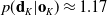 $p(\textbf{d}_K | \textbf{o}_K ) \approx 1.17$ and
  $p(\textbf{d}_K | \bar{\textbf{o}}_K )=2$ ! Indeed, the prior knowledge on the occupancy value
  $p(\textbf{o}_K)$ does not agree with the inverse model, that is
  $p(\textbf{o}_K| \textbf{d}_K )<p(\textbf{o}_K)$ and
  $p(\textbf{o}_K| \bar{\textbf{d}}_K )<p(\textbf{o}_K)$, which is of course not logical. All in all, using the inverse model directly is not a limitation in itself, if carefully handled. Nevertheless, we find that explicitly introducing forward sensor models is much needed.
2.3. Binary state model limitations
It is well understood that the occupancy field discards the distribution and density of reflectors inside a cell. Indeed, only two states are allowed, which greatly limits the description of the environment. As a direct consequence, binary state occupancy maps do not permit to compare occupancy values across multiple cells, which have not been probed evenly. For instance, the posterior probability of a cell might be high (i.e., close to 1) either because the cell reflectivity is high or because the cell has a moderate amount of reflectors, but has been probed intensively. In other words, in Eq. (2), the rate of convergence for two occupied (or unoccupied) cells depend on their respective true intrinsic probabilities  $\alpha(\textbf{d}|W)$, which are usually not equal. Using binary occupancy maps alone results in the loss of much of the information gathered from lidar recordings and prevents quantitative analysis of the robot potential knowledge of the environment.
Overall, Bayesian schemes applied to classic occupancy grid suffer from several drawbacks. While occupancy fields are extensively used, we find that the lack of a well-founded forward model limits map quality assessment. On the other hand, a deterministic physics model is simply too costly to compute for onboard applications and we must find alternative approaches.
3. Space Mapping and Data Assimilation
The probabilistic nature of the forward model  $p( \textbf{d} | \textbf{o} )$ cannot be solely explained by uncertainties on our lidar instrument readings or by random time-evolving events. It is in reality best explained by the underlying physics of lidar ray interaction with the occupancy grid map. Indeed, the use of a single model parameter with a binary value per cell in a spatially discretized model fails to describe natural environments with complex distributions of reflectors (i.e., leaves, particles, fractal features, local dynamic events) [Reference Deschaud, Prasser, Dias, Browning and Rander14]. We thus have to deal, in addition to model inaccuracies and instrument uncertainties, with cells which seem to randomly reflect or let lidar ray pass through. This apparent random behavior is precisely what
  $p( \textbf{d} | \textbf{o} )$ and
  $p( \textbf{d} | \bar{\textbf{o}}_K )$ encompass. Having a probabilistic forward model can appear counterintuitive given the deterministic nature of the physics at hand. Thankfully, it is possible to formally derive its mathematical expression from the underlying physics using Bayes’ rule and space mapping as detailed in this section.
3.1. Related studies
Statistical models are introduced in Bayesian and statistical inference literature through model selection issues [Reference Burnham and Anderson20,Reference Cox21]. This approach finds its roots in the historical need for models associated to complex systems, such as biology and human sciences, where deterministic models are not available. We choose here to focus on probabilistic forward models induced from deterministic models. Consequent efforts have been put to tackle discretization and model reduction issues in the inverse problem community [Reference Pavliotis and Stuart22–Reference Cotter, Dashti, Robinson and Stuart24]. One of the most elegant approaches to tackle many parameterization or discretization issues is Bayesian inversion on functional spaces, which has already been extensively studied (e.g., refs. [Reference Fitzpatrick25,Reference Stuart26]). However, this alternative is not always easy to manipulate and in practice, many engineering applications perform a discretization and space mapping step ahead as in refs. [Reference Burgard, Fox, Hennig and Schmidt13,Reference Hornung, Wurm, Bennewitz, Stachniss and Burgard19]. In addition, functional inverse problems usually require a numerical implementation of the forward model, which implicitly involves model reduction and discretization [Reference Stuart26,Reference Tarantola and Nercessian27]. This numerical implementation step may be of little consequence if the discretization is adapted to the geometry of the model parameter field. Nevertheless, we usually do not have access to this geometry since the model parameter field is unknown. The literature is rich in works that explore issues related to resulting model errors in inverse problems [Reference Huttunen, Kaipio and Somersalo29–Reference Kennedy and O’Hagan31]. Recent work by Watson et al. [Reference Watson and Holmes32] on approximate models have highlighted the potential of acknowledging parameterization issues. In the field of inverse problem and optimization, the concept of space mapping has been used since the mid 1990s as recalled by Bandler et al. [Reference Bandler and Cheng33]. The original idea of space mapping was to map the problem using coarse model parameters to speed up the process of finding the global maximum on the original space. However, as we will see, space mapping can be used to directly infer information on the new space. Studies of parameterization, probabilistic model errors, and optimization naturally relate to space mapping issues discussed in this section.
3.2. Bayesian data assimilation framework
We define here data assimilation as the task of recovering information on model parameter  $\textbf{m}$ given (i) recorded measurements
  $\textbf{D}$, (ii) a sampling distribution (i.e., forward model)
  $p(\textbf{d}|\textbf{m})$, and (iii) some prior knowledge on the model parameter
  $p(\textbf{m})$. We further assume that measurements are uncertain (for instance, due to instrument limitations) and can be derived from true data
  $\textbf{d}$ using the sampling density
  $p(\textbf{D}|\textbf{m} , \textbf{d})$. Bayes’ rule then allows us to write,
 \begin{equation}\begin{aligned}p(\textbf{m},\textbf{d}|\textbf{D}) = p( \textbf{m} ) \, \frac{p(\textbf{d}|\textbf{m}) \, p(\textbf{D}|\textbf{m} , \textbf{d})}{p(\textbf{D})}\end{aligned}\end{equation}
  $p(\textbf{m},\textbf{d}|\textbf{D})$ corresponds to the usual joint posterior probability density on the model parameter and true data. This expression is the solution of our general inverse problem and is the basis of Bayesian data assimilation algorithms (e.g., refs. [Reference Jaynes17,Reference Kolmogorov34]). Since measurements
  $\textbf{D}$ usually fully depend on their associated true value
  $\textbf{d}$, we can write
  $p(\textbf{D}|\textbf{m} , \textbf{d}) = p(\textbf{D}|\textbf{d})$. This probability density induces a well-behaved density on
  $\mathfrak{D}$ since
  $\textbf{D}$ is known. Note that in occupancy grid mapping,
  $p(\textbf{D}|\textbf{d})$ corresponds to the lidar reading accuracy and
  $\int_{\mathfrak{D}} p(\textbf{D}|\textbf{d}) \, p(\textbf{d}|\textbf{m}) \, d\mu_{\mathrm{D}}$ corresponds to the sensor model. As previously stated, sensor models in the literature such as Thrun et al. [Reference Thrun, Burgard and Fox16] do not correspond to the probability to generate a lidar data point given an occupancy map. They rather correspond to the probability to generate a lidar data point given a real-world map, which results in probability densities not living on the same space. In addition, recorded data, (i.e., power over time) when using lidar instruments, are not used directly but post-processed to return time stamps. The associated data space in Eq. (4) is thus different from the raw lidar sensor recordings. We shall now discuss how to address these issues using space mapping and illustrate the importance of using appropriate forward models.
3.3. Space mapping
We loosely define space mapping as the mapping of a data assimilation problem on a joint probability space  $\mathfrak{D} \times \mathfrak{M}$ to a new joint probability space
  $\tilde{\mathfrak{D}} \times \tilde{\mathfrak{M}}$. More explicitly, space mapping allows to transport probability densities from
  $\mathfrak{D} \times \mathfrak{M}$ to
  $\tilde{\mathfrak{D}} \times \tilde{\mathfrak{M}}$ (see Fig. 2). In order to perform space mapping, we need to introduce a measurable function
  $\varphi: \, \mathfrak{M} \times \mathfrak{D} \to \tilde{\mathfrak{M}} \times \tilde{\mathfrak{D}}$, which acts as the map. In practice, data and model spaces are often different in nature, and hence it is common to provide distinct maps for each space. Consequently, we introduce two measurable functions
  $\varphi_\mathrm{M}: \, \mathfrak{M} \to \tilde{\mathfrak{M}}$ and
  $\varphi_\mathrm{D}: \, \mathfrak{D} \to \tilde{\mathfrak{D}}$, which act as maps on model spaces and data spaces, respectively. It is then possible to explicitly map outcomes of sample spaces associated to
  $\mathfrak{D}$ and
  $\mathfrak{M}$ to outcomes of sample spaces associated to
  $\mathfrak{D}$ and
  $\mathfrak{M}$, that is,
 \begin{equation}\begin{aligned}\tilde{\textbf{m}} &= \varphi_\mathrm{M} \left(\textbf{m}\right) \\[3pt]\tilde{\textbf{d}} &= \varphi_\mathrm{D} \left(\textbf{d}\right)\end{aligned}\end{equation}
 Similarly, it is possible to use this mapping to transport probability densities  $p( \textbf{m} )$,
  $p(\textbf{D}|\textbf{d})$, and
  $p(\textbf{d}|\textbf{m})$ living on
  $\mathfrak{D}$ and
  $\mathfrak{M}$ (see Eq. (7)) to probability densities living on
  $\tilde{\mathfrak{D}}$ and
  $\tilde{\mathfrak{M}}$. These new probability densities are often referred to as mapped probability densities. Using mapped probability densities results in the following new data assimilation problem on
  $\tilde{\mathfrak{D}} \times \tilde{\mathfrak{M}}$:
 \begin{equation}\begin{aligned}p(\tilde{\textbf{m}},\tilde{\textbf{d}}|\textbf{D}) = p( \tilde{\textbf{m}} ) \, \frac{p(\tilde{\textbf{d}}|\tilde{\textbf{m}}) \, p(\textbf{D}|\tilde{\textbf{d}})}{p(\textbf{D})}\end{aligned}\end{equation}
where
 \begin{equation}p(\textbf{D}) = \int_{\tilde{\mathfrak{M}}} p(\tilde{\textbf{m}}) \, \left( \int_{\tilde{\mathfrak{D}}} p(\textbf{D}|\tilde{\textbf{d}}) \, p(\tilde{\textbf{d}}|\tilde{\textbf{m}}) \, d\mu_{\tilde{\mathrm{D}}} \right) d\mu_{\tilde{\mathrm{M}}}\end{equation}
 Note that in Eq. (9),  $p( \tilde{\textbf{m}} )$,
  $p(\textbf{D}|\tilde{\textbf{d}})$, and
  $p(\tilde{\textbf{d}}|\tilde{\textbf{m}})$ correspond to mapped probability densities
  $p( \textbf{m} )$,
  $p(\textbf{D}|\textbf{d})$, and
  $p(\textbf{d}|\textbf{m})$, respectively. On the other hand, the posterior probability
  $p(\tilde{\textbf{m}},\tilde{\textbf{d}}|\textbf{D})$ associated to the new data assimilation problem in Eq. (9) is usually not equal to the mapping of the posterior probability density
  $p(\textbf{m},\textbf{d}|\textbf{D})$ from Eq. (7). In other words, the mapping of products is usually not equal to the product of mappings.
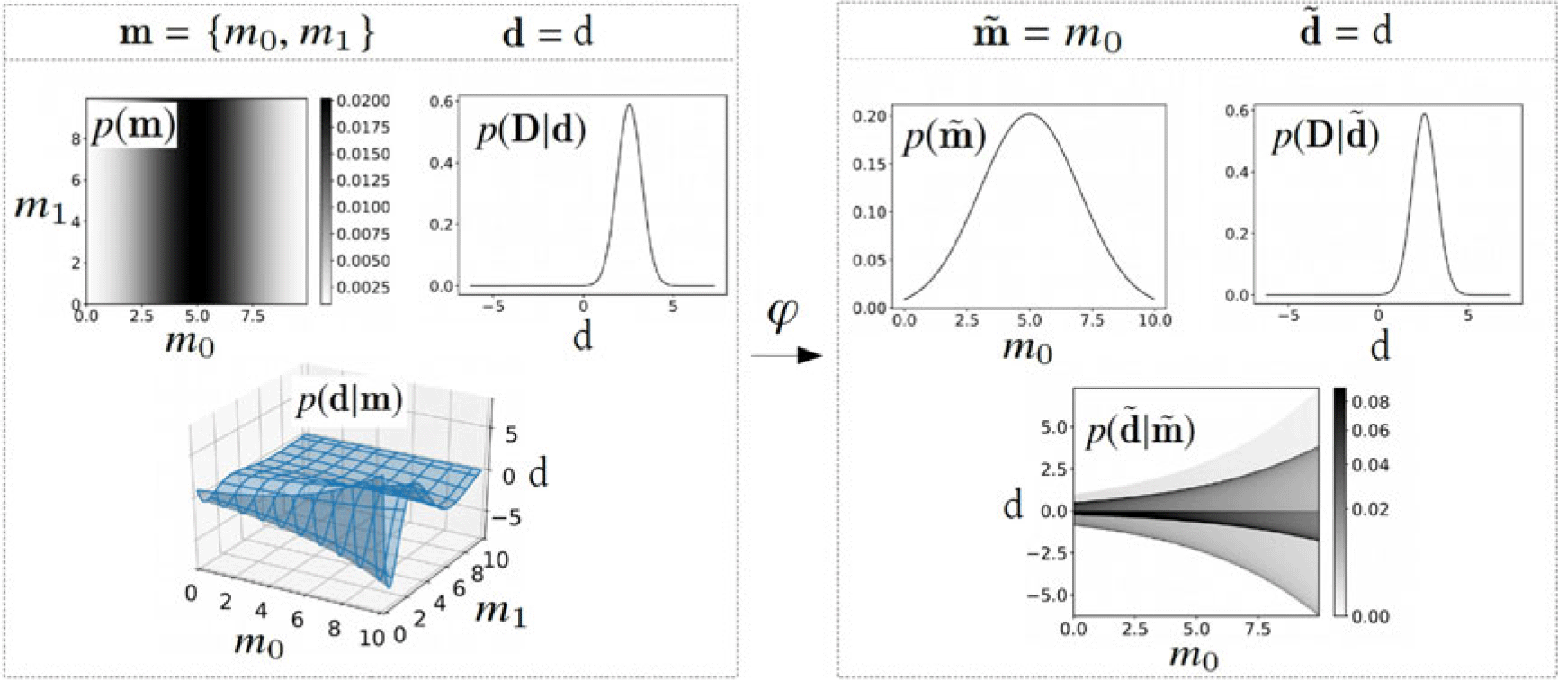
Figure 2. Model reduction is a special case of space mapping. In this example, the model parameter space is reduced from two dimensions to one dimension. Probability densities associated to the new model parameter space are displayed on the right. Note that in this example, the forward model is such that  $p(\textbf{d}|\textbf{m}) \propto \delta(\textbf{d} - g(\textbf{m}))$. This example is further detailed in Section 3.4
In order to derive an analytical expression of  $p(\tilde{\textbf{m}},\tilde{\textbf{d}}|\textbf{D})$, we need to provide analytical expressions of mapped probability densities
  $p( \tilde{\textbf{m}} )$,
  $p(\textbf{D}|\tilde{\textbf{d}})$, and
  $p(\tilde{\textbf{d}}|\tilde{\textbf{m}})$. We let
  $\mathscr{D}$ and
  $\mathscr{M}$ be measurable subsets of
  $\sigma$-algebras associated to
  $\mathfrak{D}$ and
  $\mathfrak{M}$. We further endow data and model spaces with homogeneous measures,
  $\mu_{\mathrm{D}}$ and
  $\mu_{\mathrm{M}}$, respectively [18,Reference Halmos35]. More specifically, we let
  $\mu_{\tilde{\mathrm{M}}}$ be the pushforward of
  $\mu_{\mathrm{M}}$ by
  $\varphi_\mathrm{M}$, that is
  $\mu_{\tilde{\mathrm{M}}}[\tilde{\textbf{m}} ] = \mu_{\mathrm{M}}[\varphi_\mathrm{M}^{-1}(\tilde{\textbf{m}} ) ]$. In a similar fashion, we explicitly let the pushforward measure by
  $\varphi_\mathrm{D}$ of
  $\mu_{\mathrm{D}}$ be
  $\mu_{\tilde{\mathrm{D}}}$. We can now detail the mapped forward model
  $p(\tilde{\textbf{d}}|\tilde{\textbf{m}})$,
 \begin{align}&\int_{\tilde{\mathscr{M}}} \int_{\tilde{\mathscr{D}}} p(\tilde{\textbf{d}}|\tilde{\textbf{m}}) \, d\mu_{\tilde{\mathrm{D}}} \, d\mu_{\tilde{\mathrm{M}}} \nonumber\\&\quad = \int_{\varphi_{\mathrm{M}}^{-1} \left(\tilde{\mathscr{M}} \right)} \int_{\varphi_{\mathrm{D}}^{-1} \left(\tilde{\mathscr{D}} \right)} p \big(\varphi_{\mathrm{D}}(\textbf{d})|\varphi_{\mathrm{M}}(\textbf{m}) \big) \, d\mu_{\mathrm{D}} \, d\mu_{\mathrm{M}} \end{align}
 \begin{align}&\quad = \int_{\varphi_{\mathrm{M}}^{-1} \left(\tilde{\mathscr{M}} \right)} \int_{\varphi_{\mathrm{D}}^{-1} \left(\tilde{\mathscr{D}} \right)} p(\textbf{d}|\textbf{m}) \, d\mu_{\mathrm{D}} \, d\mu_{\mathrm{M}}\nonumber\end{align}
 We can further derive mapped probability densities  $p( \tilde{\textbf{m}} )$ and
  $p(\textbf{D}|\tilde{\textbf{d}})$ of
  $p( \textbf{m} )$ and
  $p(\textbf{D}|\textbf{d})$, respectively. We let
  $\tilde{\mathscr{M}}$ and
  $\tilde{\mathscr{D}}$ be measurable subsets of
  $\tilde{\mathfrak{M}}$ and
  $\tilde{\mathfrak{D}}$, respectively such that,
 \begin{align}\int_{\tilde{\mathscr{M}}} p( \tilde{\textbf{m}} ) \, d\mu_{\tilde{\mathrm{M}}}= \int_{\varphi_{\mathrm{M}}^{-1} \left(\tilde{\mathscr{M}} \right)} p \big( \varphi_{\mathrm{M}} ( \textbf{m} ) \big) \, d\mu_{\mathrm{M}} = \int_{\varphi_{\mathrm{M}}^{-1} \left(\tilde{\mathscr{M}} \right)} p(\textbf{m}) \, d\mu_{\mathrm{M}}\end{align}
and
 \begin{equation}\begin{aligned}\int_{\tilde{\mathscr{D}}} p(\tilde{\textbf{D}}|\tilde{\textbf{d}}) \, d\mu_{\tilde{\mathrm{D}}}= \int_{\varphi_{\mathrm{D}}^{-1} \left(\tilde{\mathscr{D}} \right)} p \big( \textbf{D}|\varphi_\mathrm{D}(\textbf{d}) \big) \, d\mu_{\mathrm{D}}= \int_{\varphi_{\mathrm{D}}^{-1} \left(\tilde{\mathscr{D}} \right)} p(\textbf{D}|\textbf{d}) \, d\mu_{\mathrm{D}} \, d\mu_{\mathrm{D}}\end{aligned}\end{equation}
 Note that  $\mu_{\tilde{\mathrm{M}}}$ is not required to be the pushforward of
  $\mu_\mathrm{M}$ by
  $\varphi_\mathrm{M}$ and
  $\mu_{\tilde{\mathrm{D}}}$ is not required to be the pushforward of
  $\mu_\mathrm{D}$ by
  $\varphi_\mathrm{D}$. It is nevertheless practical to enforce these conditions to avoid additional terms as discussed in ref. [Reference Halmos35], p. 164. For regular smooth maps, which admit derivatives and local inverse, previous equations are equivalent to the usual change of variable. In particular, we can write locally
  $\mu_{\tilde{\mathrm{M}}} \big(\varphi_{\mathrm{M}} ( \textbf{m} ) \big) \, \big| \det J_{\varphi} \big| = \mu_{\mathrm{M}}(\textbf{m})$, where
  $J_{\varphi}$ is the local Jacobian of
  $\varphi_{\mathrm{M}}$. Using the new probability densities on the new joint space, we can derive the posterior probability density
  $p(\tilde{\textbf{m}},\tilde{\textbf{d}}|\textbf{D})$ given our knowledge on the new joint space using Eq. (9). Since we are only interested in recovering information on the model space, we marginalize the previous equation such that,
 \begin{equation}\begin{aligned}p(\tilde{\textbf{m}}|\textbf{D}) = \frac{p( \tilde{\textbf{m}} )}{p(\textbf{D})} \, \int_{\tilde{\mathfrak{D}}} p(\tilde{\textbf{d}}|\tilde{\textbf{m}}) \, p(\textbf{D}|\tilde{\textbf{d}}) \, d\mu_{\tilde{\mathrm{D}}}\end{aligned}\end{equation}
  $\int_{\tilde{\mathfrak{D}}} p(\tilde{\textbf{d}}|\tilde{\textbf{m}}) \, p(\textbf{D}|\tilde{\textbf{d}}) \, d\mu_{\tilde{\mathrm{D}}}$ corresponds to the well-known likelihood function. In essence,
  $p(\tilde{\textbf{m}}|\textbf{D})$ corresponds to the posterior probability density using (i) the pushforward of the forward model, (ii) the pushforward of our prior knowledge on the model parameter, and (iii) the pushforward of our instrument uncertainties. It usually differs from the pushforward of the posterior
  $p(\textbf{m},\textbf{d}|\textbf{D})$ of the inverse problem on the original space since the conjunction of the pushforwards is not the same as the pushforward of the conjunction. In practice, we often use probability densities on the new joint space without having access to their corresponding probability densities on the original space. Thus, probability densities
  $p( \tilde{\textbf{m}} )$ and
  $p(\textbf{D}|\tilde{\textbf{d}})$ can be chosen independently from any prior model parameter and instrument knowledge on the original space. On the other hand, the original forward model
  $p(\textbf{d}|\textbf{m})$ is often known from deterministic physical laws, but deriving
  $p(\tilde{\textbf{d}}|\tilde{\textbf{m}})$ can be a tedious task. It is common to use the original forward model in place of its corresponding new forward model. Since deterministic physical laws induce Dirac-like probability distribution densities, this permutation yields inaccurate results in many cases and we strongly advocate against it. We now choose to discuss two interesting cases, which involve deterministic forward models.
3.4. Model reduction
We assume that we are dealing with Riemannian manifolds probability spaces, where we can explicitly write  $$(d{\mu _{\rm{D}}}/d\textbf{d}){\mkern 1mu} d\textbf{d} = d{\mu _{\rm{D}}}$$ and
  $$(d{\mu _{\rm{M}}}/d\textbf{m}){\mkern 1mu} d\textbf{m} = d{\mu _{\rm{M}}}$$. We further assume that the forward model is
  $p(\textbf{d}|\textbf{m}) = \delta(\textbf{d} - g(\textbf{m})) \, \left( d\mu_\mathrm{D}/d\textbf{d} \right)^{-1}$, where
  $\delta$ denotes the Dirac distribution and g is a known operator from
  $\mathfrak{M}$ to
  $\mathfrak{D}$ such that
  $\textbf{d}=g(\textbf{m})$. Note that g is not necessarily linear and is often implicitly defined through a set of differential equations. Finally, we let the map
  $\varphi_\mathrm{D}$ be the identity, that is
  $\textbf{d} = \tilde{\textbf{d}}$.
 \begin{equation}\begin{aligned}\int_{\tilde{\mathscr{D}}} \int_{\tilde{\mathscr{M}}} p(\tilde{\textbf{d}}|\tilde{\textbf{m}}) \, d\mu_{\tilde{\mathrm{M}}} \, d\mu_{\tilde{\mathrm{D}}}= \int_{\mathscr{D}} \int_{\varphi_{\mathrm{M}}^{-1} \left(\tilde{\mathscr{M}} \right)} \delta(\textbf{d} - g(\textbf{m})) \, \frac{d\mu_\mathrm{M}}{d \textbf{m}} \, d\textbf{m} \, d \textbf{d}\end{aligned}\end{equation}
 In essence,  $\int_{\tilde{\mathscr{D}}} \int_{\tilde{\mathscr{M}}} p(\tilde{\textbf{d}}|\tilde{\textbf{m}}) \, d\mu_{\tilde{\mathrm{M}}} \, d\mu_{\tilde{\mathrm{D}}}$ is the number of models
  $\textbf{m}$ that satisfies both
  $\{\textbf{d} =g(\textbf{m})|\textbf{d} \in \mathscr{D}\}$ and
 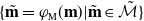 $\{\tilde{\textbf{m}}=\varphi_\mathrm{M}(\textbf{m})|\tilde{\textbf{m}} \in \tilde{\mathscr{M}} \}$. Of course, since we are not dealing with discrete sets, the term number should be understood here as a measure of volumes. If we further assume g to be a smooth regular invertible function, the previous equation reduces to a mere change of variable, that is,
 \begin{equation}\begin{aligned}\int_{\tilde{\mathscr{D}}} \int_{\tilde{\mathscr{M}}} p(\tilde{\textbf{d}}|\tilde{\textbf{m}}) \, d\mu_{\tilde{\mathrm{M}}} \, d\mu_{\tilde{\mathrm{D}}}= \int_{\mathscr{D}} \sum_{k=1}^{n(\textbf{d})} \frac{d\mu_\mathrm{M}}{d \textbf{m}} \big(g^{-1}_k(\textbf{d})\big) \, \bigg|\det \frac{dg}{d\textbf{m}}\big(g^{-1}_k(\textbf{d})\big)\bigg|^{-1} \, d \textbf{d}\end{aligned}\end{equation}
 where  $g^{-1}_k(\textbf{d})$ are the
  $n(\textbf{d})$ solutions in
  $\textbf{m}$ for the equation
  $g(\textbf{m})=\textbf{d}$ with
  $\textbf{m} \in \varphi_{\mathrm{M}}^{-1} \left(\tilde{\mathscr{M}} \right)$. Figure 3 shows a basic example, where the model parameter space is reduced from two to one dimensions. In this example, homogeneous measure densities
  $d\mu_\mathrm{D}/d\textbf{d}$ and
  $d\mu_\mathrm{M}/d\textbf{m}$ are set to constant. Figure 3(a) corresponds to the usual deterministic model, whereas Fig. 3(b) corresponds to the resulting forward model density obtained using Eq. (15). The presence of a hidden variable combined with a fully deterministic original forward model induces an obviously new nondeterministic forward model density, as shown in Fig. 3(b). In Fig. 4, we display probability densities associated to a typical data assimilation problem conducted on the joint space
  $\mathfrak{M} \times \mathfrak{D}$ and its associated data assimilation problem on the new joint space
  $\tilde{\mathfrak{M}} \times \mathfrak{D}$. We use a constant prior density associated to model parameter
  $m_1$ for both data assimilation problems. This choice is motivated by the fact that the homogeneous density (which is constant) represents best the lack of knowledge on
  $m_1$. The resulting posterior density is shown in Fig. 4(b). Since the prior probability density over
  $m_1$ is proportional to the homogeneous measure, we obtain identical marginal posterior probability densities for
  $m_0$ regardless of the data assimilation problem used (see Fig. 4(d)), which is in agreement with common sense expectations. In practice, model reduction often arises in multi-scale setups when seeking a low-dimensional homogenized approximation
  $\tilde{\textbf{m}}$ of model parameter
  $\textbf{m}$ as discussed by Pavliotis and Stuart [Reference Pavliotis and Stuart22]. Homogenization theory introduces, for instance, an effective model parameter
  $\tilde{\textbf{m}}$, which allows to derive a homogenized forward operator
  $\tilde{g} \left(\tilde{\textbf{m}} \right)$. As a result, the forward model
  $p(\tilde{\textbf{d}}|\tilde{\textbf{m}})$ is often approximated by a Gaussian distribution [Reference Nolen, Pavliotis and Stuart36] on the data space centered on
  $\tilde{g} \left(\tilde{\textbf{m}} \right)$ with covariance
  $\textbf{C}_T$. Since
  $\textbf{C}_T$ is independent from model parameter
  $\tilde{\textbf{m}}$, everything appears as if the original probabilistic forward model information is being transferred onto the data space. While this can be very useful, one must, however, bear in mind that we are really dealing with a probabilistic forward model and that in general, probabilistic forward models are not equivalent to model parameter independent random variables [Reference Kaipio and Somersalo37,Reference Lassas, Saksman and Siltanen38].
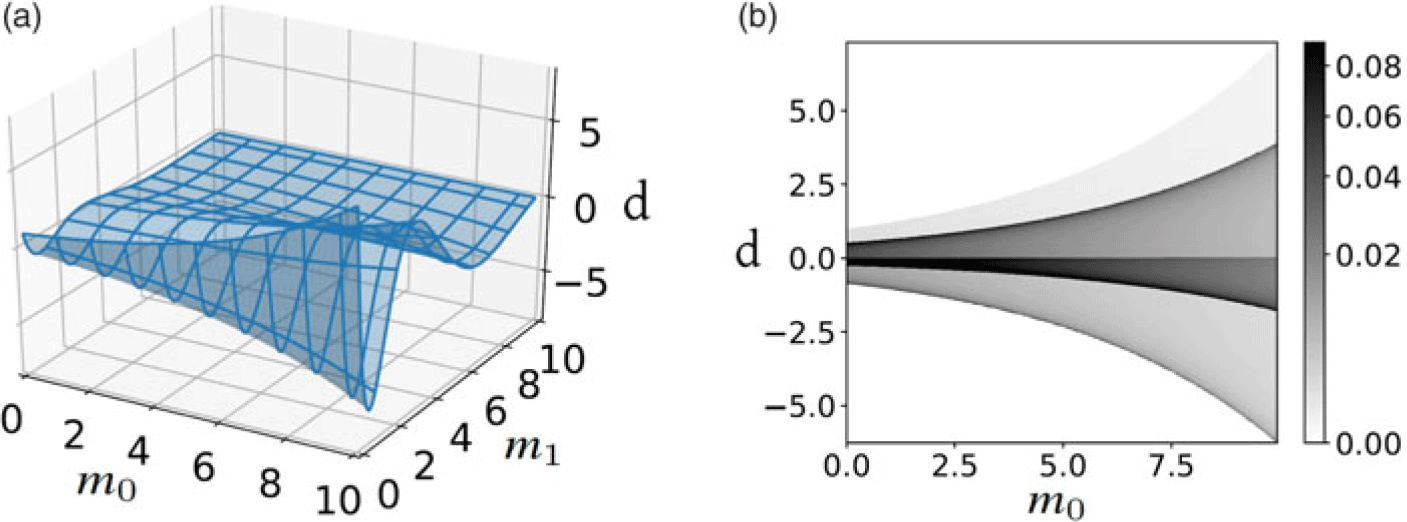
Figure 3. (a) Deterministic forward function g where  $\textbf{d}=g(\textbf{m})$ with
  $\textbf{m} = \{m_0,m_1\}$. (b) Nondeterministic forward probability
  $p(\textbf{d}|m_0)$ resulting from the mapping
  $\tilde{\textbf{m}} = m_0$. Note:
  $\tilde{\textbf{d}}=\textbf{d}$. Homogeneous measures are set to constant in this example
Figure 4. Probability densities associated to the forward operator and mapping ares described in Fig. 3. (a) Probability density  $p(\textbf{D}|\tilde{\textbf{d}}) \, p(\tilde{\textbf{m}})$ over the joint space
  $\tilde{\mathfrak{M}} \times \mathfrak{D}$. (b) Posterior probability density is associated to
  $p(\tilde{\textbf{m}},\tilde{\textbf{d}}|\textbf{D})$. (c) Marginal posterior probability density is associated to
  $p(\textbf{m}|\textbf{D})$. This density is obtained using the marginal over
  $\textbf{d}$ of
  $p(\textbf{m},\textbf{d}|\textbf{D})$. (d) Marginal posterior probability densities is associated to
  $p(m_0|\textbf{D})$ (dashed line with circular markers) and
  $p(m_0|\textbf{D})$ (continuous line)
The second case of interest is what we shall call discretization. Following Kaipio and Somersalo [Reference Kaipio and Somersalo37] and Alekseev and Navon [Reference Alekseev and Navon23], we now let  $\mathfrak{M}$ be a separable Hilbert space. Consequently, the unknown
  $\textbf{m}$ is a vector on
  $\mathfrak{M}$. To study discretization, we let
  $\tilde{\mathfrak{M}} \subset \mathfrak{M}$ be such that
  $\dim (\tilde{\mathfrak{M}}) = n$ where its n elements
  $\{ \phi_j\}$ are orthonormal. We further define the discretization operator
  $\Phi $ such that
  $\tilde{\textbf{m}} = \sum_{j=1}^{n} \langle \textbf{m}, \phi_{j} \rangle \phi_{j} = \Phi (\Phi)^T \textbf{m}$. Discretization clearly appears as a specific case of space mapping where
  $\varphi_\mathrm{M} (\textbf{m}) = \Phi (\Phi)^T \textbf{m}$. Consequently, performing discretization within an data assimilation problem framework often results in dealing with what we have described as probabilistic forward models. In the literature, it is common to write
  $\textbf{d} = \tilde{g} \left(\tilde{\textbf{m}} \right) + w$ in place of explictely using the concept of probabilistic forward model [Reference Kennedy and O’Hagan31,Reference Kaipio and Somersalo37]. w corresponds to a random variable which accounts for discretization errors. Of course, the addition of this model parameter-dependent random variable to the deterministic forward model is eventually equivalent to our proposed probabilistic forward model.
For a given problem, model space mapping induces a new data assimilation problem on a new joint space. The forward model associated to this new problem is different from the forward model associated to the original data assimilation problem. Understanding the mapping from one domain to another is essential to design proper inference algorithms. Space mapping appears thus critical when using coarse model parameters, as in robotics lidar data assimilation.
4. Lidar Data Assimilation Using a New Probabilistic Forward Model
Using results from the previous section, we propose to introduce a new model parameter to replace the occupancy field. Since our goal is to perform onboard real-time mapping, the forward model associated to this new model parameter must result in a cheap update rule.
4.1. Space mapping
It is well understood that lidar measurements are best modeled by radiative transfer [Reference Chandrasekhar39]. In the case of lidar used in mobile robotics, radiative transfer physics parameters reduce to the absorption field  $\mu_a(\textbf{x},t,\nu)$, the scattering field
  $\mu_s(\textbf{x},t,\nu)$, and the scattering phase function
 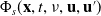 $\Phi_s(\textbf{x},t,\nu,\textbf{u},\textbf{u}')$.
  $\textbf{u}$ and
  $\textbf{u}'$ are unit vectors indicating directions of propagation.
  $\nu$ is the usual lidar light frequency and t indicates time dependency of parameter fields. These parameter fields are defined over a bounded region of interest
  $\Omega$, a connected open region in 3D, where
  $\textbf{x} \in \Omega$. Prescribed parameter fields on
  $\Omega$ yield deterministic lidar measurements, which correspond to the received power over time. Figure 5 shows a simple schematic representation associated to this model. A lidar ray is shown propagating through a field of discrete scatterers (dark blue) in a homogeneous low absorbing medium (light blue). The deterministic forward model associated to radiative transfer is usually represented through a set of differential equations (see [Reference Chandrasekhar39], Eq. (48), p. 9). The initial conditions of this set of equations are determined by the lidar instrument.
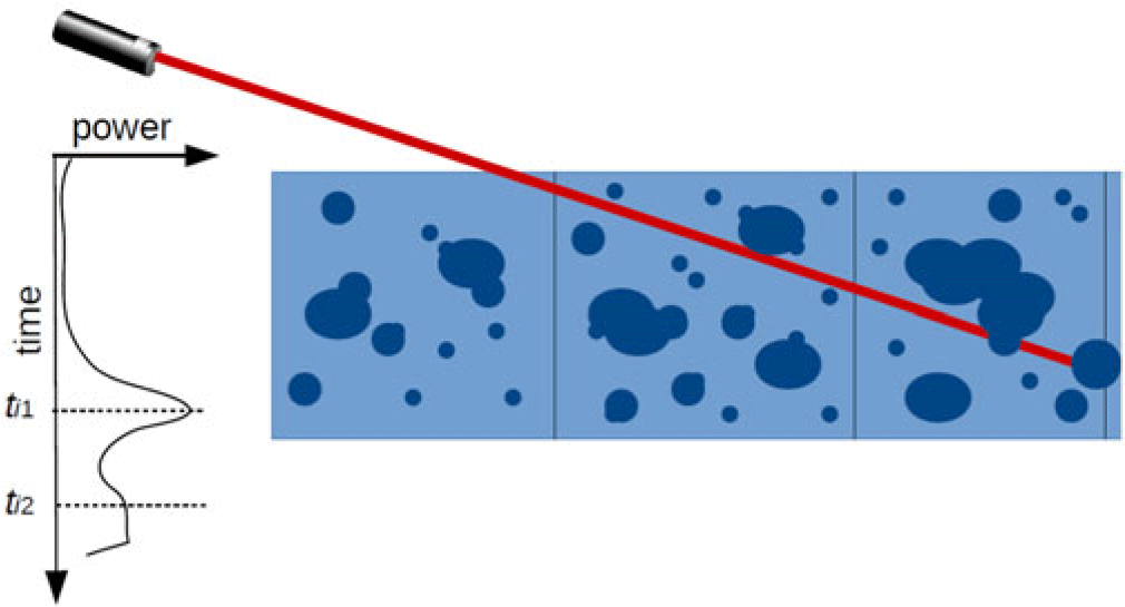
Figure 5. Schematic representation of lidar ray propagating in a scattering environment. Bins are associated to the spatial discretization  $\Omega = \cup_{K=1}^N \mathcal{V}_K$. Recorded lidar power over time is indicated as well as the associated returned times as discussed in the text
It is common to use a set of time values (see Fig. 5) in place of received power over time. Time values correspond usually to either multiple strong power peaks or to the first arrival. We let  $\{t_{i1}\}_{i \in I}$ be the set of first arrival times (i.e., one first time arrival per lidar ray). Following notations used in Section 3, we let the measurable data space associated to the received power over time be
  $\mathfrak{D}$ and the data space associated to first time value
  $t_{i1}$ be
  $\tilde{\mathfrak{D}}$ (see Fig. 6). In other words, we let
  $\{\tilde{\textbf{d}}_i\}_{i \in I}=\{t_{i1}\}_{i \in I}$. The function
  $\varphi_{\mathrm{D}}$ from lidar recorded power to first arrival times corresponds to the data map. We choose to use first arrivals, which corresponds to one time stamp return per lidar ray, for practical reasons. Indeed, while current lidar data can provide several time stamps per ray (first arrival, strongest peaks, etc.), deriving an analytical expression for the posterior probability using multiple time stamps can be tedious and would require additional work.
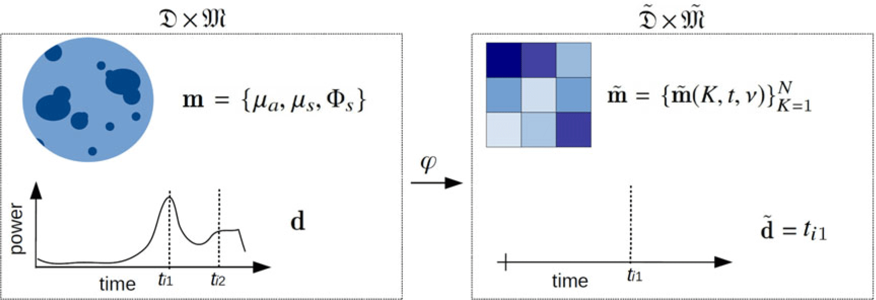
Figure 6. Proposed space mapping in this study. The function  $\varphi$ maps from (a) the original model parameter space associated to radiative transfer and data space associated to recorded lidar power to (b) the new model parameter space
  $\{\tilde{\textbf{m}}(K,t,\nu)\}_{K=1}^N$ and the new first arrival time data space
Similarly, we let the model parameter space associated to  $\mu_a$,
  $\mu_s$, and
  $\Phi_s$ be
  $\mathfrak{M}$, such that a point on this space is
 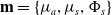 $\textbf{m}=\{\mu_a,\mu_s,\Phi_s\}$. We impose
  $\mathfrak{M}$ to be measurable, which will allow us to use results from the previous section. It is reasonable to impose such condition as
  $\mu_a$,
  $\mu_s$, and
  $\Phi_s$ do not account for small scale quantum physics. Solving radiative transfer equations is impractical in real-time data assimilation. In addition, while backscattering and radiative transfer encompass the physics at hand, local space and time discrepancies of model parameter field values and lidar setup can greatly affect recorded data as discussed by Deschaud et al. [Reference Deschaud, Prasser, Dias, Browning and Rander14]. It is thus preferable to recover local statistics in place of the model parameter field values. We let the spatial region of interest
  $\Omega$ be a set of N contiguous volume elements
  $\mathcal{V}_K$ such that
  $\Omega = \cup_{K=1}^N \mathcal{V}_K$ (see Fig. 5). Using this discretization, we introduce a new model parameter
 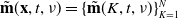 $\tilde{\textbf{m}}(\textbf{x},t,\nu) = \{\tilde{\textbf{m}}(K,t,\nu)\}_{K=1}^N$, which corresponds to the local probability that a lidar ray propagating over a unit distance is not backscattered (i.e., transparent medium). Conceptually, this probability can be derived from the local average distance traveled by a lidar ray, which is also known as the mean free path. The mean free path
  $L_K$ in cell K can be obtained by averaging over all incoming directions and over all incoming points on the cell boundary and corresponds to
  $-1/ \log \left( \tilde{\textbf{m}} \right)$. It is thus possible to explicitly derive the mapping function
  $\varphi_\mathrm{M}$ associated to the new model parameter. The new model parameter space associated to
  $\tilde{\textbf{m}}$ is denoted
  $\tilde{\mathfrak{M}}$ by the following notations from Section 3 (see Fig. 6).
So far, the concept of occupancy does not appear. To circumvent this issue, it is possible to define the degree of occupancy of a cell. Remembering that  $\tilde{\textbf{m}}(\textbf{x},t,\nu)$ is the probability that no backscattering occurs along a unit lidar ray path, we define the degree of occupancy field as the local complementary event of
  $\tilde{\textbf{m}}(\textbf{x},t,\nu)$. With the prescribed discretization, this simply means that the degree of occupancy in cell K is
  $1-\tilde{\textbf{m}}_{K}(t,\nu)$ (see Table 1). Note that with our definition, model parameters in Fig. 1 are of course unit dependent. In addition, working with
  $\tilde{\textbf{m}}$, the mean free path or the degree of occupancy is strictly equivalent (see Section 4.4).
Table 1. Parameters definition
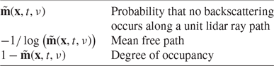
Mean free paths and first arrival times are not the only model and data parameters that can be used in lidar data assimilation. For instance, in Appendix A, we provide an augmented formulation of the problem where data records both time of flight and reflected amplitudes. We thus introduce an additional model parameter associated to the local reflected lidar power. One can also design complex new model parameters, which more closely relate to the underlying radiative transfer physics parameters. However, in this work, we specifically chose new model parameters, which yield simple data assimilation algorithm, directly usable for onboard mobile robot applications.
In the following sections, we purposely omit the frequency dependency  $\nu$ and time dependency of model parameter fields.
4.2. A new probabilistic forward model
Now that we have defined a new model parameter and data space, and we need to derive the new associated forward model. In order to derive the new forward model, we make several assumptions regarding the problem at hand. First, we assume that laser light propagates as a 1D ray, not as a cone or as a tube (see Fig. 7). Indeed, using a volumetric representation of laser rays would require to take into consideration the cross section of scatterers, the reflectivity of scatterers as well as the instrument sensitivity, which would considerably increase the complexity of the problem at hand and would not allow for onboard real-time computations. Second, we discard multiple reflections and additional scattering of laser light. This amounts to a first-order approximation and will allow to derive an analytical expression for the new forward model as we will see. We let  $\textbf{r}_i$ denote a 3D unit vector representing, for a given measurement lidar measurement, the direction along the laser ray (see Fig. 7) and we let c be the speed of light in the probed medium. Finally, we let
  $\textbf{x}_{0,i}$ be the lidar location (see Fig. 7).
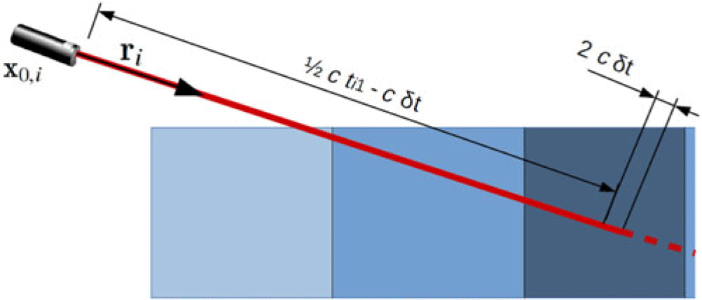
Figure 7. Schematic representation of lidar ray propagating in the new model parameter field 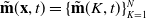 $\tilde{\textbf{m}}(\textbf{x},t) = \{\tilde{\textbf{m}}(K,t)\}_{K=1}^N$ (see Fig. 5)
Using these assumptions and notations, the probability that no reflection occurs from the lidar instrument to the point of reflection for the  $i{\rm th}$ ray with its associated first arrival time
  $t_{i1}$ can be expressed as
 \begin{equation}\begin{aligned}\exp \left( \int_0^{t_{i1}/2-\delta t} \log \big( \tilde{\textbf{m}}(\textbf{x}_{0,i}+c \, t \, \textbf{r}_i) \big) \, c \, dt \right)\end{aligned}\end{equation}
  $\tilde{\textbf{m}}(\textbf{x}_{0,i}+c \, t \, \textbf{r}_i)$ corresponds to the field value at
  $\textbf{x}=\textbf{x}_{0,i}+c \, t \, \textbf{r}_i$ and where
  $\delta t$ represents an infinitely small time increment. In order to derive this expression, we simply use the definition of the new model parameter
  $\tilde{\textbf{m}}$, which corresponds to the local probability that a lidar ray propagating over a unit distance is not backscattered. Similarly, it is possible to derive the probability that backscattering occurs at the tip of the ray. We define the tip of the ray as
  $[\textbf{x}_{0,i}+ c \, (t_{i1}/2-\delta t) \, \textbf{r}_i,\textbf{x}_{0,i}+ c \, (t_{i1}/2+\delta t) \, \textbf{r}_i]$. The probability that backscattering occurs at the tip of the ray is then,
 \begin{equation}\begin{aligned}1-\exp \left( \int_{t_{i1}/2-\delta t}^{t_{i1}/2+\delta t} \log \big( \tilde{\textbf{m}}(\textbf{x}_{0,i}+c \, t \, \textbf{r}_i) \big) \, c \, dt \right)\end{aligned}\end{equation}
 The probability of observing a first arrival time  $t_{i1}$ for the
  $i{\rm th}$ lidar ray is simply the conjunction (i.e., product) of (i) the probability that no reflection occurs from the lidar instrument to the point of reflection (see Eq. (17)) and (ii) the probability that backscattering occurs at the tip of the ray (see Eq. (18)). Letting
  $\delta t \to 0$, we can write,
 \begin{equation}\begin{aligned}&p(t_{i1}|\tilde{\textbf{m}}) \propto \lim_{\delta t \to 0} \,\exp \left( \int_0^{t_{i1}/2-\delta t} \log \big( \tilde{\textbf{m}}(\textbf{x}_{0,i}+c \, t \, \textbf{r}_i) \big) \, c \, dt \right) \cdot \\[3pt]&\left( 1-\exp \left( \int_{t_{i1}/2-\delta t}^{t_{i1}/2+\delta t} \log \big( \tilde{\textbf{m}}(\textbf{x}_{0,i}+c \, t \, \textbf{r}_i) \big) \, c \, dt \right) \right)\end{aligned}\end{equation}
 Using the spatial discretization  $\tilde{\textbf{m}} = \cup_{K=1}^N \tilde{\textbf{m}}_K$ and using
  $\lim_{\delta t \to 0} \, (1-\tilde{\textbf{m}}_K)^{2\delta t} (1+2 \delta t)/\delta t=-\log(\tilde{\textbf{m}}_K)$ yields,
 \begin{equation}\begin{aligned}p(t_{i1}|\tilde{\textbf{m}}) &\propto -\exp \left( \sum_{K} s_{K,i} \log \left( \tilde{\textbf{m}}_{K} \right) \right) \, \log(\tilde{\textbf{m}}_{K_i})\end{aligned}\end{equation}
  $s_{K,i}$ denotes the distance traversed by the
  $i{\rm th}$ lidar ray in cell K.
  $\tilde{\textbf{m}}_{K}$ is the scalar field value associated to cell K and
  $\tilde{\textbf{m}}_{K_{i}}$ is the scalar field value associated to the last cell traversed by the lidar ray (i.e., where backscattering occurs). Assuming independent lidar measurements from one another the resulting forward model can then be derived as
 \begin{equation}\begin{aligned}p(\{t_{i1}\}_{i \in I}|\tilde{\textbf{m}}) &\propto \prod_{i \in I} \: p(t_{i1}|\tilde{\textbf{m}})\propto \prod_{i \in I} \: -\exp \left( \sum_{K} s_{K,i} \log \left( \tilde{\textbf{m}}_{K} \right) \right) \, \log(\tilde{\textbf{m}}_{K_i})\end{aligned}\end{equation}
Appendix A details an alternative forward model, which uses reflectivity parameters in addition to the probability that no backscattering occurs along a unit lidar ray path. Adding the reflectivity parameter can be particularly useful in exploration robotics in complex environments and where mapping the environment is a primary task [Reference Rekleitis, Bedwani and Dupuis6,Reference Opromolla, Fasano, Rufino, Grassi and Savvaris7].
4.3. Posterior probability density and update rule
From a Bayesian perspective, the update rule associated to a lidar mapping algorithm corresponds to the computation of the posterior probability on the model parameter space given new recorded lidar data (i.e.,  $p(\tilde{\textbf{m}}|\{\textbf{D}_i\}_{i \in I})$). Using Eq. (21) in Eq. (14) and letting the homogeneous measures be constant over the new data space yields,
 \begin{equation}\begin{aligned}&p(\tilde{\textbf{m}}|\{\textbf{D}_i\}_{i \in I}) = p(\tilde{\textbf{m}}) \, \prod_{i \in I} \int_{0}^{t_{\max}} p(\textbf{D}_i|t_{i1}) \, p(t_{i1}|\tilde{\textbf{m}}) \, d t_{i1}\\&\propto p(\tilde{\textbf{m}}) \, \prod_{i \in I} \int_{0}^{t_{\max}} -p({\textbf{D}}_i|t_{i1}) \, \exp \left( \sum_{K} s_{K,i} \log \left( \tilde{\textbf{m}}_{K} \right) \right) \, \log(\tilde{\textbf{m}}_{K_i}) \, dt_{i1}\end{aligned}\end{equation}
 where  $t_{\max}$ is the lidar maximum recording time. Equation (22) corresponds to the update rule associated to the new forward model. It allows to update the information in each cell given recorded lidar data. Note that robot pose and lidar orientation are also parameters of the forward model (see Eq. (21)). Consequently, replacing
  $\tilde{\textbf{m}}$ in Eq. (22) with robot pose, lidar orientation parameters and field parameter
  $\tilde{\textbf{m}}$ allows to jointly inverse these different parameters. The new forward model thus naturally enables Simultaneous Localization And Mapping (SLAM).
Equation (22) is the general solution to our mapping problem. Unfortunately, this equation is not always practical to implement due to onboard computation resources limitation. Thankfully, the posterior probability density expression can be further simplified provided additional assumptions on prior and data uncertainty probability densities. Assuming data uncertainties are such that  $p({\textbf{D}}_i|t_{i1}) \propto \delta \left(t_{i1}-T_{i1}\right)$ and assuming uncorrelated cells such that the prior probability on the new model parameter space
  $p(\tilde{\textbf{m}})$ reduces to
  $p(\tilde{\textbf{m}}) = \prod_{K} \: p(\tilde{\textbf{m}}_K)$ allows to write,
 \begin{equation}\begin{aligned}&p(\tilde{\textbf{m}}|\{\textbf{D}_i\}_{i \in I}) = \prod_{K} \: p\left(\tilde{\textbf{m}}_K|\{\textbf{D}_i\}_{i \in I}\right)\end{aligned}\end{equation}
where
 \begin{equation}\begin{aligned}&p\left(\tilde{\textbf{m}}_K|\{\textbf{D}_i\}_{i \in I}\right) \propto p(\tilde{\textbf{m}}_K) \, \left( -\log(\tilde{\textbf{m}}_{K}) \right)^{n_K} \, \left( \tilde{\textbf{m}}_K \right)^{s_K}\end{aligned}\end{equation}
  $s_K = \sum_{i \in I} s_{K,i}$ is the cumulated distance traveled by all lidar rays in cell K and
  $n_K$ corresponds to the number of rays being reflected in cell K. While assuming uncorrelated prior densities might seem reasonable in practice, assuming no data uncertainty is of course not realistic. On the other hand, such assumption is commonly used in occupancy mapping [Reference Hornung, Wurm, Bennewitz, Stachniss and Burgard19]. The underlying reasoning is that spurious measurements on lidar instruments are statistically sparse and do not result in meaningful bias. In addition, inaccuracies regarding first arrival times are often significantly smaller than cell dimensions and consequently can be discarded. The resulting posterior density can be expressed in closed form for each cell and can be readily implemented. Having access to a closed-form expression for the posterior probability allows to significantly reduce computation costs and is very well suited for real-time onboard applications.
4.4. Constant prior probability density and mean free path parameter
Using different prior model parameter probability densities in Eq. (24) results in different update rules. Figure 8 shows posterior model parameter densities using constant prior probability densities such that,
 \begin{equation}\begin{aligned}&p\left(\tilde{\textbf{m}}_K|\{\textbf{D}_i\}_{i \in I}\right) = \frac{\left(-\log(\tilde{\textbf{m}}_{K})\right)^{n_K} \, (\tilde{\textbf{m}}_{K})^{s_K}}{n_K ! \, (s_K+1)^{-n_K-1}}\end{aligned}\end{equation}
 In such a case, the posterior probability is unimodal and admits a single maximum for  $\tilde{\textbf{m}}_K=\exp\left(-n_K/s_K \right)$. The mean and variance associated to the posterior probability density in Eq. (25) can further be obtained analytically using the following relation:
 \begin{equation}\begin{aligned}E \big[ {\tilde{\textbf{m}}_K}^z \big] = \left( \frac{s_K+1}{s_K+1+z} \right)^{n_K+1}\end{aligned}\end{equation}
 where  $z \in \mathbb{N}$. Typical probability densities associated to different values of
  $s_K$ and
  $n_K$ are shown in Fig. 8. From Fig. 8, it is clear that standard deviation decreases as
  $s_K$ and
  $n_K$ increase while their ratio remains constant. This behavior is in agreement with the expected information gain from repeated probing within a cell K. Interestingly, the mean free path value associated to the maximum likelihood (i.e.,
  $-\log \left( \exp\left(-n_K/s_K\right) \right)$) is the ratio of the sum of the distances of all ray, which is passed through the cell (i.e.,
  $s_K$) over the number of lidar ray reflected within the cell (i.e.,
  $n_K$). Hence, the best mean free path value corresponds to the intuitive result one would provide as a best estimate of the mean free path within a given cell.
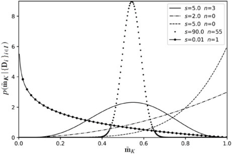
Figure 8. Posterior probability density distributions  $p(\tilde{\textbf{m}}_K|\{\textbf{D}_i\}_{i \in I})$ in cell K for different
  $s_K$ and
  $n_K$ values
All equations so far have been expressed using the local probability that a lidar ray propagating over a unit distance is not backscattered  $\tilde{\textbf{m}}$. It is, however, possible to use the local mean free path or the local degree of occupancy (see Table 1) in place of
  $\tilde{\textbf{m}}_K$. For instance, letting the local mean free path be denoted
  $L_K$ be such that
  $L_K = -1/\log(\tilde{\textbf{m}}_{K})$ and
  $\mu_{L}$ be the associated homogeneous measure then we can replace Eq. (24) with,
 \begin{equation}\begin{aligned}&p\left(L_K|\{\textbf{D}_i\}_{i \in I}\right) \propto p(L_K) \, \left(\frac{1}{L_K} \right)^{n_K} \, \exp \left( -\frac{L_K}{s_K} \right)\end{aligned}\end{equation}
 where  $p(L_K) = p(\tilde{\textbf{m}}_K) \, d \mu_{\tilde{\mathrm{M}}}/d \mu_{L}$ and
  $p(L_K|\{\textbf{D}_i\}_{i \in I}) = p(\tilde{\textbf{m}}_K|\{\textbf{D}_i\}_{i \in I}) \, d \mu_{\tilde{\mathrm{M}}}/d \mu_{L}$. In other words, using the local mean free path or the local degree of occupancy in place of
  $\tilde{\textbf{m}}_K$ does not affect forward models or data uncertainties, but requires to transport prior probability densities from one space to the other. For example, let us assume constant homogeneous measures for both
  $\tilde{\textbf{m}}_K$ and
  $L_K$ and let us further assume the prior probability
  $p(\tilde{\textbf{m}}_K)$ is constant, as shown in Fig. 8. The associated prior probability
  $p(L_K)$ is then such that
  $p(L_K) \propto d \tilde{\textbf{m}}_K/d L_K$, which yields
  $p(L_K) \propto \exp(-1/L_K)/L_K^2$. Consequently, assuming constant prior probability densities for
  $\tilde{\textbf{m}}_K$ results in assuming prior probability densities
  $p(L_K) \propto \exp(-1/L_K)/L_K^2$ for the mean free path. All in all, working with
  $\tilde{\textbf{m}}_K$, the mean free path or the degree of occupancy is strictly equivalent provided prior probabilities are carefully taken into account.
4.5. Dynamic environment
In the previous section, we have implicitly assumed the environment to be static over time. To account for dynamic environment, we use a time decay function  $f(t-t')=\exp(-|t-t'|/T)$, where T is a fixed time constant characterized by the environment dynamics and
  $t>t'$ corresponds to different times at which we acquire different independent data
  $\textbf{D}(t)$ and
  $\textbf{D}(t')$. Using this function, we let,
 \begin{equation}p(\tilde{\textbf{m}}_K(t)|\textbf{D}(t')) \propto p(\tilde{\textbf{m}}_K(t')|\textbf{D}(t'))^{f(t-t')}\end{equation}
For instance, using Eq. (28) along with Eq. (25), we can derive the following dynamic environment posterior probability density:
 \begin{equation}\begin{aligned}p \left(\tilde{\textbf{m}}_K(t)|\textbf{D}(t),\textbf{D}(t')\right)= \frac{\left(-\log(\tilde{\textbf{m}}_{K}(t))\right)^{n_K(t)} \, (\tilde{\textbf{m}}_{K}(t))^{s_K(t)}}{n_K(t) ! \, (s_K(t)+1)^{-n_K(t)-1}}\end{aligned}\end{equation}
with
 \begin{equation}\begin{aligned}&n_K(t)= n_{K}(t') \, f(t-t') + n_{K}\left(\textbf{D}(t)\right) \\[3pt]&s_K(t) = s_{K}(t') \, f(t-t') + s_K\left(\textbf{D}(t)\right)\end{aligned}\end{equation}
  $n_{K}\left(\textbf{D}(t)\right)$ corresponds to 1 or 0, depending on whether the lidar ray
  $\textbf{D}(t)$ was reflected in cell K. Similarly,
  $s_K\left(\textbf{D}(t)\right)$ corresponds to the distance traveled in cell K associated to lidar ray
  $\textbf{D}(t)$. The resulting maximum likelihood is such that
  $\tilde{\textbf{m}}_K(t)=\exp\left(-n_K(t)/s_K(t) \right)$. The time decay function allows to forget older measurements (i.e., decrease the confidence) while preserving the value of the best estimate of the degree of occupancy. If no new data are recorded, the uncertainty increases over time while the best estimate of the mean free path, that is
  $n_K(t)/s_K(t)$, remains unchanged. The different steps of the resulting algorithm are displayed in Algorithm 1.
4.6. What about occupancy parameters?
In this section, we compare results from our approach to the ones from classic occupancy grid. As discussed in Section 2, the occupancy field suffers from a lack of clear definition. In order to compare the approach detailed in this study to the occupancy field, we use the degree of occupancy of a cell which corresponds to  $1-\tilde{\textbf{m}}_K$.
We recall that the occupancy field is a binary field, where 1 locally denotes the occupied state and 0 the nonoccupied state (see Section 2). In other words, in the occupancy grid setup, a cell occupancy state is equal to 1 if it is occupied and equal to 0 otherwise. Let us now consider a simple model, where a single cubic cell of dimension  $10 \times 10 \times 10$ cm
 $^3$ is repeatedly probed by a lidar instrument. Figure 9 shows associated degree of occupancy of this cell for different lidar readings. The probability of the cell to be occupied given successive lidar measurements is detailed in Eq. (5). In Fig. 9(a), the most likely occupancy state of the cell is first 1 (i.e.,
  $p(\textbf{o}_K| \{\textbf{D}_i\}_{i \in I} )>0.5$) as the first 10 first lidar rays are reflected in the cell. Remaining lidar rays simply pass through the cell without being reflected which eventually sets the most likely occupancy state to 0 (i.e.,
  $p(\textbf{o}_K| \{\textbf{D}_i\}_{i \in I} )<0.5$).
Algorithm 1 Lidar data assimilation algorithm

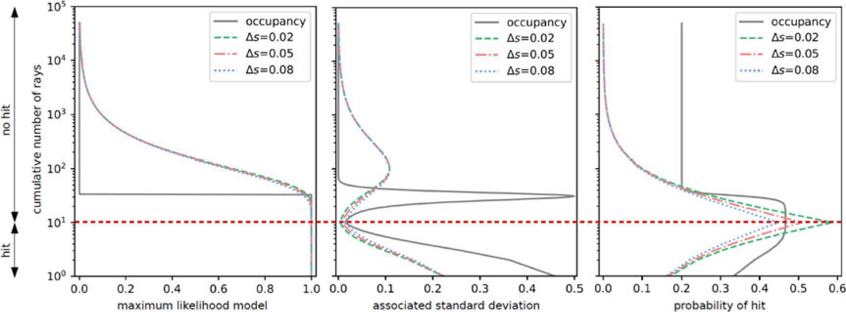
Figure 9. Evolution in a single cell of (i) the value of the model associated to the maximum likelihood (left), (ii) the associated standard deviation (center), and (iii) the probability  $p(\textbf{d}_K|\{\textbf{D}_i\}_{i \in I})$ of a ray to be reflected (i.e., hit) in the cell. Occupancy grid approach results are diplayed using a continuous line while dotted lines correspond to the degree of occupancy with our proposed approach (see legend boxes). The y-axis corresponds to the cumulated number of lidar rays being assimilated. The characteristic length of the cell is set to 10 cm. Note that
  $\Delta s$ corresponds to the update of the cumulated distance traveled through the cell (i.e.,
  $s_K$), after a single measurement. Occupancy prior is set to
  $p( \textbf{o}_K )=0.5$. We use the following values for the occupancy forward model:
  $p(\textbf{d}_K | \bar{\textbf{o}}_K )=0.2$ and
 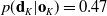 $p(\textbf{d}_K | \textbf{o}_K )=0.47$. The first 10 lidar rays are reflected (see red dotted line) while the remaining ones pass through the cell. When a lidar ray is reflected, we use different
  $\Delta s$ values (see legend box), which results in different behaviors. When a ray passes through, we set
  $\Delta s=0.1$, which corresponds to the length of the cell. After i measurements, we let
  $s_K(i)$ be the associated
  $s_K$ such that:
 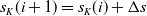 $s_K(i+1)=s_K(i) + \Delta s$
Recalling parameter definitions (see Table 1), it is possible to study the probability  $p(\textbf{d}_K|\{\textbf{D}_i\}_{i \in I})$ that a lidar ray is being reflected in a cell, that is the probability of hit in Fig. 9,
 \begin{align}&p(\textbf{d}_K|\{\textbf{D}_i\}_{i \in I}) \end{align}
 \begin{align}&= \int_{\tilde{\mathfrak{M}}_K} p(\textbf{d}_K|\tilde{\textbf{m}}_K,\{\textbf{D}_i\}_{i \in I}) \, p(\tilde{\textbf{m}}_K|\{\textbf{D}_i\}_{i \in I}) \, d \tilde{\textbf{m}}_K \end{align}
 \begin{align}&= \int_{\tilde{\mathfrak{M}}_K} \big(1- \tilde{\textbf{m}}_{K}^{s_{0K}} \big) \, \frac{\left(-\log(\tilde{\textbf{m}}_{K})\right)^{n_K} \, (\tilde{\textbf{m}}_{K})^{s_K}}{n_K ! \, (s_K+1)^{-n_K-1}} \, d \tilde{\textbf{m}}_K \end{align}
 \begin{align}&= 1-\left( \frac{s_K + 1}{s_K + s_{0K} +1} \right)^{n_K + 1}\end{align}
 where  $s_{0K}$ is the characteristic length of the cell (i.e.,
  $0.1$ in the example shown in Fig. 9). In the previous equation, we have used
  $p(\textbf{d}_K|\tilde{\textbf{m}}_K,\{\textbf{D}_i\}_{i \in I})= p(\textbf{d}_K|\tilde{\textbf{m}}_K) = 1-\tilde{\textbf{m}}_{K}^{s_{0K}}$. In the case of the occupancy grid mapping,
  $p(\textbf{d}_K|\textbf{D}) = p(\textbf{d}_K | \bar{\textbf{o}}_K ) \, p( \bar{\textbf{o}}_K|\textbf{D} ) + p(\textbf{d}_K | \textbf{o}_K ) \, p( \textbf{o}_K|\textbf{D} )$. Consequently, in occupancy grid mapping, the probability to observe lidar reflection in a cell is bounded by its forward model values
  $p(\textbf{d}_K | \bar{\textbf{o}}_K )$ and
  $p(\textbf{d}_K | \textbf{o}_K )$. In the example shown in Fig. 9, the values of the occupancy grid mapping forward model are
  $0.2$ and
  $0.47$, respectively. As the first 10 lidar rays are reflected in the cell, the probability to hit rapidly converges toward
  $0.47$. However, all remaining lidar rays pass through the cell. This induces a decrease in the probability to hit which eventually converges to
  $0.2$. On the contrary, our proposed approach allows the probability to hit to freely converge to any values between 0 and 1. In the example, the probability to hit first converges toward 1 as the number of lidar rays being reflected in the cell increases. It then converges toward 0 as all lidar rays pass through the cell. Overall, convergence rates for occupancy parameter and degree of occupancy parameter are in agreement with the analytical forms of their respective update rules. It is important to bear in mind that for the most likely degree of occupancy to converge toward 0, its associated mean free path must converge toward infinity. For example, in Fig. 9, the first 10 rays are being reflected in the cell. For the most likely degree of occupancy to reach
  $0.63$ (i.e., mean free path equals to 1), this requires at least
  $10/0.1=100$ rays to pass through the cell as observed in Fig. 9. In other words, small changes in the value degree of occupancy can be associated to large changes in the mean free path value. Standard deviations are further shown in Fig. 9. We recall that the standard deviation associated to the occupancy model described in Section 2 is equal to
  $p(\textbf{o}_K|\{\textbf{D}_i\}_{i \in I}) \, \left( 1- p(\textbf{o}_K|\{\textbf{D}_i\}_{i \in I}) \right)$. The standard deviation associated to our new model can be simply derived using Eq. (26).
Main advantages of the proposed approach can be summarized as follows. Unlike occupancy grid mapping, there is no need to specify ad hoc values associated to the forward model. Prior knowledge on the mean free path and measurements are sufficient to update our knowledge on the mean free path. The mean free path is clearly defined with regard to the underlying radiative transfer parameters, and so is the degree of occupancy. In addition, the posterior probability density over the mean free path allows quantitative comparison between cells and across maps.
4.7. A practical case
This section presents results obtained using real lidar data in an outdoor environment. Lidar data were acquired on a mobile robot platform (customized SUMMIT-XL from Robotnik) in an outdoor environment with a Velodyne Puck sensor placed on top (see Fig. 10). We used  $\sim1$ s acquisition time from which
  $\sim320,000$ lidar rays were recorded. Using a short window of time for lidar acquisition allows to identify better individual rays on the map (see Fig. 12). Robot location and orientation were estimated using an onboard inertial sensor. The resulting short trajectory of the robot is approximated by a thick red line in Figs. 11 and 12.

Figure 10. Experimental setup for lidar data acquisition. The lidar sensor is highlighted in red on the picture. The lidar sensor operates with a  $360^{\circ}$ vertical field of view (
 $\sim0.2^{\circ}$ angular resolution) and a
  $\pm 15^{\circ}$ vertical field of view (
 $2.0^{\circ}$ angular resolution)
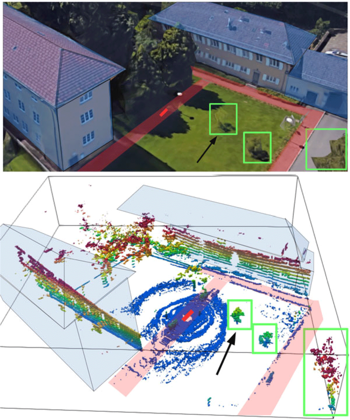
Figure 11. Top: real 3D image scene are obtained using Google Maps. Credits: Images @2019, Google, Landsat/Copernicus, Data SIO, NOAA, U.S. Navy, NGA, GEBCO, Map Data, Âl2019 GeoBasis-DE/BKG (Âl2009), Google Germany. Bottom: elevation. Cells displayed are cells with most likely degree of occupancy values larger than  $0.5$
$0.5$
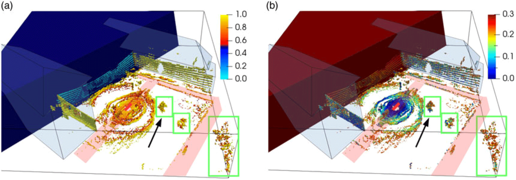
Figure 12. Reconstructed scene derived from lidar data ( $\sim320,000$ rays) using the proposed algorithm. Coloring is associated to the degree of occupancy value of the cells (i.e., most likely degree of occupancy left and standard deviation right)
Figure 12 shows maps obtained using the approach detailed in this paper. More explicitly, for this example, Algorithm 4.5 was used. The original scene is shown in Fig. 11. It corresponds to a highly diverse environment with buildings, windows, roads, mown grass, and different types of trees. Buildings, pedestrian tracks, and landmark vegetation are highlighted in the different figures. The black arrow in Figs. 11 and 12 points to the tree used in Fig. 13. On the elevation map, the ground (grass and pedestrian track) can be clearly identified by the blue cells surrounding the robot path. Note that lidar returns from two persons, in the back and in front of the robot, can be seen in the robot’s vicinity in both the elevation map and Fig. 12. The spatial discretization used is a 3D rectilinear grid. Cubic voxels are of size  $10 \times 10 \times 10 \, \mathrm{cm}^3$, which is identical to the cell size used in Fig. 9. The dimension of the scene displayed is
  $55 \times 55 \times 12 \, \mathrm{m}^3$. Most likely degrees of occupancy and degree of occupancy standard deviations are shown in Fig. 12. We recall that the most likely degree of occupancy corresponds, for each cell, to
  $1-\exp(-n_K/s_K)$. We also recall that the standard deviation associated to the occupancy model described in Section 2 is equal to
  $p(\textbf{o}_K|\{\textbf{D}_i\}_{i \in I}) \, \left( 1- p(\textbf{o}_K|\{\textbf{D}_i\}_{i \in I}) \right)$. The standard deviation associated to our new model can be simply derived using Eq. (26).

Figure 13. Details of the tree highlighted by the black arrow are shown in Figs. 11 and 12. In (a), (b), and (c), cells displayed are cells with most likely degree of occupancy values larger than  $0.5$. In (d), (e), and (f), cells displayed are cells with probabilities of being occupied larger than
  $0.5$. (a) and (d): most likely degree of occupancy. (b) and (e): degree of occupancy standard deviation. (c) and (f): probability of the occupancy state to be 1 (i.e.,
  $p(\textbf{o})$)
As expected, the degree of occupancy in each cell converges toward 0 where no reflectors are present (i.e,. empty cells). It converges toward nonzero in partially occupied or occupied cells according to the degree of reflectivity of the cell (walls, trees, grass, etc.). Associated standard deviation decreases in cells, which have been probed most effectively, by incorporating the amount of information gained from recursive probing. This can be clearly seen on the grass and concrete around the robot as well on building walls and tree trunks. Cells which have not been probed are visible in Fig. 12 on the slice and the edge of the clipped area. For instance, windows mostly act as transparent cells since returns from lidar data correspond to corridor walls and roofs. The wall facing the robot in the bottom left building contains several windows, which can be clearly seen in Figs. 11 and 12. Since these cells have not been probed, the probability density of the degree of occupancy is set to constant. This results in a degree of occupancy standard deviation of approximately  $0.29$ (dark red in Fig. 12(b)). For visualization purpose, we have arbitrarily set the associated most likely degree of occupancy of these cells to
  $0.5$ (dark blue on the slice in Fig. 12(a)). The probability density of the degree of occupancy in each cell K only depends on the cumulated ray distance cell value
  $s_K$ and on the cumulated number of hits
  $n_K$. The most likely degree of occupancy used for visualization in Fig. 12 is obtained by simply computing
  $1-\exp(-n_K/s_K)$ and the standard deviation.
In practice, the map structure obtained using our proposed forward model is nearly identical to any other map structure obtained using classic occupancy algorithm (see Algorithm 4.5). Major reflectors such as walls, floors, vegetation yield high probabilities of being occupied as well as high degrees of occupancy. However, partially occupied cells converge to either occupied or unoccupied in a classic approach while their degree of occupancy will converge toward any value between 0 and 1. It is important to recall that the occupancy value in a given cell converges either to 0 or 1 as the amount of information increases infinitely (see Eq. (2)). As a result, differences can be observed locally, especially in vegetated areas.
Figure 13 offers a detailed insight as to how algorithms operate on partially occupied cells due to vegetation. In the top row (i.e., Fig. 13(a), (b), and (c)), cells displayed are cells with most likely degree of occupancy values larger than  $0.5$. In the bottom row (i.e., Fig. 13(d), (e), and (f)), cells displayed are cells with probabilities of being occupied larger than
  $0.5$. Figure 13(a) corresponds to the view in Figs. 12(a) while 13(b) corresponds to 12(b). Note that in Fig. 13, the back of the tree is facing opposite from the robot. Consequently, lidar rays being reflected on leaves from the back of the tree must have passed through the front leaves and branches. From Fig. 13, it is possible to verify that our algorithm accounts well for partially occupied cells. Most likely degrees of occupancy range from
  $0.5$ to
  $0.8$ in cells occupied by leaves while cells occupied by denser vegetation, such as the trunk or branches, display most likely degree of occupancy values closer to 1. On the other hand, the occupancy value, as defined in Section 2, converges toward 0 in cells occupied by leaves and converges toward 1 in cells occupied by the tree trunk and branches. As a result, partially occupied cells are simply set as either occupied or unoccupied in classic occupancy mapping, and much of the information from lidar data are eventually lost.
One of the main asset of our algorithm lies also in the ability to properly relate degree of occupancy values to physics properties. Interestingly, standard deviations in cells with leaves are higher than in the trunk cells. This behavior is in agreement with our equations and with Fig.9. Overall, most likely degree of occupancy values and occupancy values are in agreement with equations detailed in this paper and follow the trends shown in Fig. 9. Using degree of occupancy parameter in place of occupancy parameter results in a precious information gain on the environment. In practice, autonomous agents’ decision-making process can benefit from this additional knowledge, for instance, when assessing traversability, especially in vegetated areas. Figure 13 further highlights limitations of occupancy mapping when sparse reflectors are present in the map. For example, setting partially occupied cells as empty or occupied can result in collision, impairment or suboptimal path planning.
The proposed data assimilation algorithm requires to cast lidar rays in the grid and fruther requires to compute the update rule in intersected cells (see Algorithm 4.5). Classic occupancy grid algorithms also requires to cast lidar rays in the grid and to compute the posterior probability in intersected cells. Consequently, computation time and memory load are expected to be fairly identical for both algorithms. In terms of memory load, algorithms require to allocate sufficient memory for grid representation and cell data. In classic occupancy grid, stored data in an intersected cell corresponds to the posterior probability which can be represented efficiently using a float number per intersected cell. In the new proposed approach, the posterior probability is fully characterized by the cumulative distance traveled as well as the number of hits. These can be represented efficiently using a float number and an integer per intersected cell. The memory load is thus not significantly different for both algorithms. Figure 14 shows run times obtained with classic occupancy mapping and our mapping algorithm. For these experiments, the number of lidar rays (i.e.,  $\sim320,000$) and the volume of the scene (i.e.,
  $55 \times 55 \times 12 \, \mathrm{m}^3$) were kept constant, but the grid resolution was incrementally changed from
  $10 \, \mathrm{cm}$ to
  $1.2\,\mathrm{m}$. For instance,
  $0.1 \, \mathrm{m}$ grid resolution (i.e.,
  $10 \times 10 \times 10 \, \mathrm{cm}^3$ cell dimensions) corresponds to the grid used in Figs. 11, 12, and 13. The total run time for a given resolution is the sum of both ray casting time and grid update time. It is important to stress that while run times depend on data assimilation algorithms, they are also very dependent on data structures and on the overall quality of the implementation. For instance, queries to find intersected cells greatly depend on the grid representation. Similarly, grid update times can often be reduced using sparse data structures. In terms of hardware, all run times were evaluated on a single core of a laptop CPU (Intel Core i5-7300HQ, 2.5 GHz). Both classic occupancy grid mapping and our own algorithm share an identical ray casting core. Both algorithms were implemented using a home developed code in C++ relying on a dense grid and on dense arrays for data storage. Note that our implementation is not well suited for large-scale problems or real-time onboard applications. For real-time onboard applications, more efficient data structure relying on sparse arrays or spatial hierarchy such as octrees can be used [Reference Hornung, Wurm, Bennewitz, Stachniss and Burgard19]. Such data structures can significantly speed up ray casting and cell data access. They also scale better as the environment volume or resolution increases. Nevertheless, independently of the implementation, it is legitimate to argue from Fig. 14 that the main bottleneck in terms of run times for both algorithms is ray casting and not the update rule. Slight differences in ray casting run times between both algorithms can be explained by the need to compute geometric distances with the new proposed approach, which is not needed in classic occupancy mapping. Similarly, differences in grid update run times can be mostly explained by the need to maintain and update geometric distances in probed cells in the first case and not in the latter. All in all, Fig. 14 indicates that the additional knowledge gained from using degree of occupancy parameter requires similar computation costs when compared to occupancy mapping.

Figure 14. Run times associated to lidar data assimilation for different grid resolutions. (a) Ray casting time. (b) Grid update time
5. Conclusion
The need for coarse maps of the environment, combined with lidar instrument’s high sensitivity, makes onboard lidar data assimilation on mobile robots a challenge from the physics perspective. Nevertheless, this study introduces a new probabilistic forward model with new model parameters using radiative transfer, space mapping, and Bayesian data assimilation. Results show that it is possible to preserve low computation costs while also maintaining a clear relation between map parameters and material parameters (i.e., mean free paths and reflectivity). Having access to an analytic expression of the forward model further allows to work with multiple parameters such as map parameters, but also lidar instrument parameters and robot pose. Hence, using an explicit expression for the forward model offers the possibility in the future to perform Simultaneous Localization And Mapping (SLAM) tasks. In addition, explicitly using map parameters with a forward model can be useful to compare robustness of algorithms based on material parameters and approximations used in each algorithm. Mapping increasingly realistic material parameters increases computation and memory loads. As a result, the approach detailed in this study does not aim at replacing current algorithms, but rather intends to fill a niche in robotic exploration where unknown and unstructured environments require robust algorithms and where material mapping is a primary task. Such scenarios include, for instance, planetary exploration robots [Reference Rekleitis, Bedwani and Dupuis6,Reference Lee, Kommedal, Horchler, Amoroso, Snyder and Birgisson8] and unmanned aerial vehicles flying in complex environments [Reference Opromolla, Fasano, Rufino, Grassi and Savvaris7,Reference Braga40]. Material parameters can also be helpful to improve autonomous agents’ decision-making process in obstacle avoidance and trajectory planning by projecting more information in the map [Reference Shaukat, Blacker, Spiteri and Gao41–Reference Khelloufi, Achour, Passama and Cherubini43]. Currently, the approach described in this paper would benefit from additional work. For instance, alternative parameters, which better account for heterogeneous scatterers and material absorption should be considered. Absorption is particularly critical for autonomous vehicles operating underwater or at sea [Reference Braga40,Reference Filisetti, Marouchos, Martini, Martin and Collings44]. Going beyond first arrival and using returned lidar power over time could also be investigated in order to take advantage of all the information collected. The ability to map material parameters should eventually also be a strong asset when conducting onboard or offline data fusion.
Acknowledgements
This work was partly supported by the joint research project MUSKETIER in a grant to A.Z. funded by the German Ministry of Research and Education, BMBF (FKZ: 01IS5001B). Much of this work was conducted within the School of Computer Science, Eberhard Karls University of Tübingen, Tübingen, Germany. We gratefully acknowledge Sebastian Buck and Goran HuskiĆ for helping with lidar data acquisition.
Conflicts of Interests
The authors declare none.
Appendix A. Deriving Eq. (2)
We study the evolution of the occupancy parameter for a given cell K as the number of lidar data grows to infinity. We use as a starting point Eq. (5), which can be derived from Bayes’ rule. We let  $n(\textbf{d})$ be the number of lidar rays associated to measurement
  $\textbf{d}$ in cell K. We recall that we assume
  $\textbf{d} \in \mathfrak{D}$. For the sake of simplicity, we first assume
  $\mathfrak{D}$ is discrete such that
  $\textbf{d}$ can take L different values, that is
  $\mathfrak{D}=\{\textbf{d}_l\}_{l \in [1,L]}$. Equation (5) now reads,
 \begin{equation}\begin{aligned}&p(\textbf{o}_K| \{\textbf{D}_i\}_{i \in [1,N]} )= \left( 1 + \frac{ 1- p(\textbf{o}_K) }{p(\textbf{o}_K)} \, \prod_{l=1}^L \left( \frac{ p( \textbf{d}_l | \bar{\textbf{o}}_K ) }{p( \textbf{d}_l | \textbf{o}_K )} \right)^{n(\textbf{d}_l)} \right)^{-1}\end{aligned}\end{equation}
 where  $\sum_{l=1}^{L} n(\textbf{d}_l) = N$ and
  $n(\textbf{d}_l)$ is the number of measurements
  $\{\textbf{D}_i\}_{i \in [1,n(\textbf{d}_l)]}$ such that
  $\textbf{D}_i=\textbf{d}_l$. We can also write,
 \begin{equation}\begin{aligned}p(\textbf{o}_K| \{\textbf{D}_i\}_{i \in [1,N]} ) = \left( 1 + \frac{ 1- p(\textbf{o}_K) }{p(\textbf{o}_K)} \, A ^N \right)^{-1}\end{aligned}\end{equation}
where
 \begin{equation}\begin{aligned}A = \exp \left( \sum_{l=1}^L \frac{n(\textbf{d}_l)}{N} \, \log\frac{ p( \textbf{d}_l | \bar{\textbf{o}}_K ) }{p( \textbf{d}_l| \textbf{o}_K )} \right)\end{aligned}\end{equation}
 As N goes to infinity, we can use the definition of the intrinsic probability  $\alpha(\textbf{d}|W)$, which is the probability to generate a single lidar measurement
  $\textbf{d}$ given the real world W. We deduce that
  $\lim_{N \to \inf} n(\textbf{d}_l)/N = \alpha(\textbf{d}_l|W)$. Using the limit in Eq. (A2), we can now write,
 \begin{equation}\begin{aligned}\lim_{N \to \inf} p(\textbf{o}_K| \{\textbf{D}_i\}_{i \in [1,N]} ) = \lim_{N \to \inf} \left( 1 + \frac{ 1- p(\textbf{o}_K) }{p(\textbf{o}_K)} \, A ^N \right)^{-1}\end{aligned}\end{equation}
where
 \begin{equation}\begin{aligned}A = \exp \left( \sum_{l=1}^L \alpha(\textbf{d}_l|W) \, \log \frac{ p( \textbf{d}_l | \bar{\textbf{o}}_K ) }{p( \textbf{d}_l| \textbf{o}_K )} \right)\end{aligned}\end{equation}
Finally, using a continuous data manifold in place of discrete data manifold yields Eq. (2).
B. Lidar Aata Assimilation Using a Reflectivity Field
Following the work of Levinson and Thrun [Reference Levinson and Thrun15], we propose to augment model parameters with the reflectivity field. The data are now composed of a time stamp  $t_{i1}$ along with its associated recorded reflected power
  $a_{i}$. In order to account for this additional information, we add a new parameter space
  $\mathfrak{R}$ to which we associate a new field, which is the reflectivity field
  $\varrho \left(a, \textbf{x}\right)$. This field corresponds to the local probability of the media to reflect a fraction a of the incoming power when the lidar ray is reflected along a unit lidar ray path. For the sake of simplicity, we discard absorption in the model, although it could be taken into account if we assume constant absorption along the lidar ray (see Fig. 5). We now introduce the following associated probabilistic forward model, which is a slightly modified version of the one detailed in Eq. (21),
 \begin{align}&p(t_{i1},a_{i}|\tilde{\textbf{m}},\varrho) \propto \prod_{i \in I} \: \varrho \left(a_i, \textbf{x}_{0,i}+ \frac{1}{2} \, c \, t_{i1} \, \textbf{r}_i\right) \nonumber\\[3pt]&\exp \left( \int_0^{t_{i1}/2-\delta t} 2 \, \log \big( \tilde{\textbf{m}}(\textbf{x}_{0,i}+c \, t \, \textbf{r}_i) \big) \, c \, dt \right) \cdot \end{align}
 \begin{align}& \left( 1- \exp \left( \int_{t_{i1}/2-\delta t}^{t_{i1}/2+\delta t} \log \big( \tilde{\textbf{m}}(\textbf{x}_{0,i}+c \, t \, \textbf{r}_i) \big) \, c \, dt \right) \right)\nonumber\end{align}
 Recalling the prescribed spatial discretization on  $\Omega$, we introduce the cell-dependent parameter
  $\varrho_{K}$ associated to a given cell K. We further choose to discretize the local probability density
  $\varrho_{K}(a_i)$ such that for
  $a_i \in {[a_j,a_{j+1}]}$,
  $\varrho_{K}(a_i)= \varrho_{j,K}$.
 \begin{equation}\begin{aligned}&p(t_{i1},a_{i}|\tilde{\textbf{m}},\varrho) \propto \prod_{i \in I} \: -\exp \left( \sum_{K} s_{K,i} \log \left( \tilde{\textbf{m}}_{K} \right) \right) \, \log(\tilde{\textbf{m}}_{K_i}) \, \varrho_{j,K_i}\end{aligned}\end{equation}
Using homogeneous priors, assuming uncorrelated cells and no measurement uncertainty, it is possible to follow the same steps as in Section 4.3 to finally obtain,
 \begin{equation}\begin{aligned}p \left(\{\tilde{\textbf{m}}_K,\{\varrho_{j,K}\}_{j \in J}|\{\textbf{D}_i\}_{i \in I} \right) \propto \prod_{K} \: \left[ p \left(\{\tilde{\textbf{m}}_K,\{\varrho_{j,K}\}_{j \in J}\right) \, \left( -\log(\tilde{\textbf{m}}_{K}) \right)^{n_{K}} \, \tilde{\textbf{m}}_{K}^{s_{K}} \, \prod_{j \in J} {\varrho_{j,K}}^{n_{j,K}} \right]\end{aligned}\end{equation}
 where  $n_{j,K}$ denotes the number of rays being reflected in the cell K with reflected power
  $a \in {[a_j,a_{j+1}]}$.
  $s_{K}$ denotes the cumulated length of all rays going through cell K. The posterior probability density now provides estimation of two independent sets of parameters for each cell K: (i)
  $\tilde{\textbf{m}}_{K}$ and (ii)
  $\{ \varrho_{j,K} \}_{j \in J}$. Let us further assume constant prior probability density
 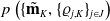 $p \left(\{\tilde{\textbf{m}}_K,\{\varrho_{j,K}\}_{j \in J}\right)$. Estimating
  $\tilde{\textbf{m}}_{K}$ has already been detailed in Eq. (24). In addition, it is then easy to show that
  $\{ \varrho_{j,K} \}_{j \in J}$ admits a maximum at
 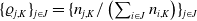 $\{ \varrho_{j,K} \}_{j \in J}=\{ n_{j,K}/ \left(\sum_{i \in J} n_{i,K}\right) \}_{j \in J}$. This maximum corresponds to the usual best estimate for data binning histograms.
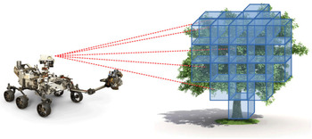


 Open access