


1. Introduction
In the last decade, small-sized drones have been rapidly developed and widely employed in many civilian applications (Floreano & Wood Reference Floreano and Wood2015; Yao, Wang & Su Reference Yao, Wang and Su2016). With the tremendous success of the relevant industry and applications of drones, the development of urban air mobility vehicles with larger sizes and weights has attracted interest (Rajendran & Srinivas Reference Rajendran and Srinivas2020; Donateo et al. Reference Donateo, de Pascalis, Strafella and Ficarella2021). However, one likely limiting factor of the development will be the annoying noise pollution during operations of the vehicles in urban regions (Al Haddad et al. Reference Al Haddad, Chaniotakis, Straubinger, Plötner and Antoniou2020; Watkins et al. Reference Watkins, Burry, Mohamed, Marino, Prudden, Fisher, Kloet, Jakobi and Clothier2020). Multiple rotors are often used in these vehicles to provide the needed forces and to realise manoeuvred flights. Consequently, the rotor operations can generate significant aerodynamic noise containing tonal and broadband contents.
Many studies have been conducted to understand the mechanisms of rotor noise generation. A few pioneering and landmark studies linking noise emission with aerodynamic flow variables were performed by Gutin (Reference Gutin1948), Deming (Reference Deming1937), Deming (Reference Deming1940), Arnoldi (Reference Arnoldi1956), Lowson (Reference Lowson1965), Lowson & Ollerhead (Reference Lowson and Ollerhead1969), Garrick & Watkins (Reference Garrick and Watkins1953) and Hubbard (Reference Hubbard1953), among others. A systematic approach to analysing the rotor noise is based on an acoustic analogy, which was initiated by Lighthill (Reference Lighthill1952) in unbounded flows and extended to problems with static boundaries by Curle (Reference Curle1955) and moving surfaces by Ffowcs Williams & Hawkings (Reference Ffowcs Williams and Hawkings1969) (FW-H). At low Mach numbers, the dominant noise sources are thickness noise and loading noise (Brentner & Farassat Reference Brentner and Farassat1998). In the presence of background mean flows, Goldstein (Reference Goldstein1974) proposed an acoustic analogy with an inhomogeneous convected wave equation, which was the basis for the rotor noise prediction model by Hanson & Parzych (Reference Hanson and Parzych1993). The noise sources estimations were based on flow velocities and loadings on the blade surfaces, which can be obtained from computational fluid dynamics or computational aeroacoustics (CAA). Notably, near-field aerodynamic flows are resolved and employed as inputs of the surface integration to compute sound at given observers (Jiang & Zhang Reference Jiang and Zhang2022). Usually, off-body integral solutions can suffer from spurious wave contamination if turbulent fluctuations pass through the integration surface (Wright & Morfey Reference Wright and Morfey2015), which was investigated in several recent studies (Shur, Spalart & Strelets Reference Shur, Spalart and Strelets2005; Ikeda et al. Reference Ikeda, Enomoto, Yamamoto and Amemiya2013; Zhong & Zhang Reference Zhong and Zhang2017, Reference Zhong and Zhang2018).
However, rotor noise study is still challenging because the flow states are complex. Flow transitions can exist because of considerable differences in the Reynolds number from rotor tips to hubs. In addition, a tip vortex is formed on the pressure side of the rotor blade, rolled up to the suction side and eventually shed from the surface. The shedding frequency also depends on the total velocity and blade thickness (Kurtz & Marte Reference Kurtz and Marte1970; Hubbard, Lansing & Runyan Reference Hubbard, Lansing and Runyan1971). The tip vortex shedding can cause unsteady surface pressure and, therefore, significant noise generation (Preisser, Brooks & Martin Reference Preisser, Brooks and Martin1994; Kim, Park & Moon Reference Kim, Park and Moon2019). The process is also influenced by the induced velocity of the vortex passing by the tip (George & Chou Reference George and Chou1986; Preisser et al. Reference Preisser, Brooks and Martin1994; Yung Reference Yung2000). Moreover, in flight conditions, the vortex shed from a blade interacting with the adjacent blades can produce significant noise (Yung Reference Yung2000) with varying directivity and strength (Splettstoesser et al. Reference Splettstoesser, Kube, Wagner, Seelhorst, Boutier, Micheli, Mercker and Pengel1997). For small-sized drone rotors, experiments are essential, and various studies have been conducted (Sinibaldi & Marino Reference Sinibaldi and Marino2013; Zawodny, Boyd & Burley Reference Zawodny, Boyd and Burley2016; Ning, Wlezien & Hu Reference Ning, Wlezien and Hu2017; Zhou & Fattah Reference Zhou and Fattah2017; Fattah et al. Reference Fattah, Chen, Wu, Wu and Zhang2019; Wu et al. Reference Wu, Chen, Fattah, Fang, Zhong and Zhang2020; Bu et al. Reference Bu, Wu, Bertin, Fang and Zhong2021). However, there is an issue that the results are often laboratory dependent because the noise measurements are sensitive to various factors (Wu et al. Reference Wu, Jiang, Zhou, Zhong, Zhang, Zhou and Chen2022). For example, in confined chambers, the noise measurements can suffer from the flow recirculation effect (Stephenson, Weitsman & Zawodny Reference Stephenson, Weitsman and Zawodny2019). There are other sources of uncertainty and unsteady factors due to the rotor motion and actual flying (Xu et al. Reference Xu, Sun, Ng and Schober2020).
This study aims at understanding the influence of various unsteady and uncertain factors, which can present in practice, on rotor noise emission. The acoustic impact of some factors was partly known in the past, but a comprehensive analysis using a unified framework is still favoured. First, in practical applications, the torque ripples of electric motors (to drive the rotors) can cause rotation speed fluctuation (Islam et al. Reference Islam, Husain, Fardoun and McLaughlin2007), which was shown to significantly affect drone noise (Kim et al. Reference Kim, Ko, Saravanan and Lee2021). The key reason is that the temporal variations of rotational speed can substantially increase the noise level (Wright Reference Wright1971; Mani Reference Mani1990) and alter noise spectra (Tinney & Sirohi Reference Tinney and Sirohi2018; McKay & Kingan Reference McKay and Kingan2019). Moreover, unsteadiness is inevitable in practical flying vehicles since the rotor speeds are adjusted by the real-time flight control (Davoudi et al. Reference Davoudi, Taheri, Duraisamy, Jayaraman and Kolmanovsky2020; Djurek et al. Reference Djurek, Petosic, Grubesa and Suhanek2020). Second, the rotor blades may experience oscillation (Marqués & Da Ronch Reference Marqués and Da Ronch2017), which is common for helicopters with pitch control mechanisms and an aeroelastic effect (Leishman Reference Leishman2006). For fixed-pitch rotors for drones, vibration can exist due to the use of light and cost-effective materials. Notably, the flexibility of rotor blades can cause coupled oscillations (Biot Reference Biot1940), which has been noticed for drone applications (Niemiec & Gandhi Reference Niemiec and Gandhi2017; Nowicki Reference Nowicki2017; Kuantama et al. Reference Kuantama, Moldovan, Ţarcă, Vesselényi and Ţarcă2021; Semke, Zahui & Schwalb Reference Semke, Zahui and Schwalb2021; Niemiec, Gandhi & Kopyt Reference Niemiec, Gandhi and Kopyt2022). The effect of flow-induced vibrations is also an active research area for marine propellers (Tian et al. Reference Tian, Zhang, Ni and Hua2017). However, the corresponding aeroacoustic studies are rare. Last, the inevitable manufacturing tolerance, wear and looseness in practical applications can cause the long-standing problem of mass imbalance and aerodynamic asymmetry of rotor blades (Best Reference Best1945; Darlow Reference Darlow2012; Huo et al. Reference Huo, Wang, Chen and Chen2020). The imbalance can result in structural vibration and extra noise generation (Altinors, Yol & Yaman Reference Altinors, Yol and Yaman2021; Semke et al. Reference Semke, Zahui and Schwalb2021). For drones, many studies have been conducted to detect and control the rotor imbalance effect (Bondyra et al. Reference Bondyra, Gasior, Gardecki and Kasiński2017; de Jesus Rangel-Magdaleno et al. Reference de Jesus Rangel-Magdaleno, Ureña-Ureña, Hernández and Perez-Rubio2018; Ghalamchi, Jia & Mueller Reference Ghalamchi, Jia and Mueller2019; Iannace, Ciaburro & Trematerra Reference Iannace, Ciaburro and Trematerra2019). Despite the (possibly) small amplitudes of these uncertainties and unsteadiness, the noise features will be significantly altered as sound contains only a tiny portion of the fluid energy.
It is difficult to quantify the effect of each factor experimentally because various mechanisms can coexist and be coupled in practice. Different factors can lead to similar impacts, making the exact causes indistinguishable. Capturing the instantaneous rotation speed variation and blade vibrations is also challenging for the instruments. Therefore, it is vital to understand the influence of each factor using more controllable approaches. In this view, high-fidelity numerical simulations could be helpful but are still too costly for parametric study. Therefore, theoretical analysis is still favoured to understand the key acoustic characteristics with various unsteady and uncertainty factors. The efficient computations using a unified framework will be helpful for more accurate and reliable noise assessment in complex working conditions.
For rotor noise prediction, Hanson & Parzych (Reference Hanson and Parzych1993) developed a frequency-domain model incorporating unsteady motions. Based on the model, Zhong et al. (Reference Zhong, Zhou, Fattah and Zhang2020) showed that periodic fluctuations can significantly increase the tonal noise levels at high frequencies. However, it only explained the behaviours of tones at harmonics of the blade passing frequency (BPF). For more generic applications, the unsteady motions might be transient and random, suggesting that noise computations based on time-domain formulations will be more convenient. Like other aeroacoustic problems, rotor noise computation (Farassat Reference Farassat1981, Reference Farassat1986; Farassat & Brentner Reference Farassat and Brentner1988; Farassat, Dunn & Spence Reference Farassat, Dunn and Spence1992; Casalino Reference Casalino2003) can be based on the integral solution of the FW-H equation, especially the widely used Farassat formulation 1A (Farassat & Succi Reference Farassat and Succi1980). However, most of the studies were conducted for rotors with constant rotation speed, even though unsteady flows were considered (Gennaretti, Testa & Bernardini Reference Gennaretti, Testa and Bernardini2013). For unsteady manoeuvres, e.g. in the helicopter noise study by Gennaretti et al. (Reference Gennaretti, Bernardini, Serafini, Trainelli, Rolando, Scandroglio, Riviello and Paolone2015), a nonlinear equation was solved to estimate the time delay that is dependent on observer location, flight trajectory and blade kinematics. For rotors experiencing unsteady motion, evaluating the retarded time with the temporally varied source locations is difficult. This work will make efforts to ease the computations to facilitate the parametric studies.
In the following, § 2 introduces the rotor noise computation formulations with the unsteady motions and uncertainties considered. Section 3 presents verification and validation of the computation model, followed by the parametric study of rotation speed variation, blade vibration and asymmetry effects. Section 4 discusses the aeroacoustic influence on dual rotors, and § 5 is the summary.
2. Formulations for rotor noise computation
In this work, we start from the acoustic analogy by Goldstein (Reference Goldstein1974) to compute the rotor aerodynamic noise generation
 \begin{equation} \left(\frac{1}{a_\infty^2}\frac{\mathscr{D}^2}{\mathscr{D}t^2} - \nabla^2\right)\left[p^\prime H(f)\right] =\frac{\mathscr{D}}{\mathscr{D} t}\left[Q\delta(f)\right] - \frac{\partial}{\partial x_i}\left[L_i\delta(f)\right] + \frac{\partial^2}{\partial x_i\partial x_j}\left[{\mathsf{T}}_{ij}H(f)\right], \end{equation}
where  $p^\prime$ is sound pressure, $a_\infty$ is speed of sound, $\boldsymbol {u}_\infty$ is the oncoming flow velocity and $\mathscr {D}/\mathscr {D}t = \partial /\partial t + \boldsymbol {u}_\infty \boldsymbol {\cdot }\boldsymbol {\nabla }$ is the material derivative. Also, $\delta (f)$ and $H(f)$ are the Dirac- $\delta$ function and Heaviside function with the argument of $f(\boldsymbol {x}(t))=0$ defining the blade surface geometry. The normal vector of the blade surface is $\boldsymbol {n}=\boldsymbol {\nabla } f$, and the location $\boldsymbol {x}(t)$ satisfying $f(\boldsymbol {x}(t))=0$ varies in time due to the blade rotation. The tensor ${\mathsf{T}}_{ij}$ is represented as ${\mathsf{T}}_{ij} = \rho u_iu_j + [(p-p_\infty ) - c_\infty ^2(\rho -\rho _\infty )]\delta _{ij} - \sigma _{ij},$ where $\rho$, $p$ and $u$ are the density, pressure and flow velocity. The subscript $(\ {\cdot }\ )_\infty$ means the variables in the uniform medium, $\delta _{ij}$ is the Kronecker- $\delta$ function and $\sigma _{ij}$ is the viscosity tensor. Further, $\partial ^2{\mathsf{T}}_{ij}/\partial x_i\partial x_j$ corresponds to the quadrupole noise source and can be omitted at low Mach numbers. Usually, $u_i$, $p$ and $\sigma _{ij}$ can be obtained by high-fidelity numerical simulations to evaluate $L_i$, corresponding to the aerodynamic loadings. However, for fast noise estimation, $L_i$ can be approximated as the aerodynamic forces acting on the blade surfaces. Finally, $Q = [\rho (u_j+u_{\infty,j}-v_j) + \rho _\infty (v_j - u_{\infty,j})]n_j$ corresponds to the thickness noise, and $v_j$ denotes velocity of the blade surface. At low Mach numbers, $\rho \approx \rho _\infty$ such that
 \begin{equation} Q \approx \rho_\infty u_jn_j. \end{equation}
2.1. Solution for rotor noise with unsteady motions
In this section, we introduce the solution to (2.1) for a rotor noise computation with the unsteady factors considered. Figure 1 illustrates the coordinates for both the observers  $\boldsymbol {x}=(x_1,x_2,x_3)$ and source points $\boldsymbol {y}=(y_1,y_2,y_3)$. The two coordinate systems are aligned, $(\ {\cdot }\ )_1$ is in the axial direction, and $(\ {\cdot }\ )_2$ corresponds to the direction when the rotation phase angle $\phi =0$. An observer described in the Cartesian system is related to the observer distance $r_o$, azimuthal angle $\varphi$ and polar angle $\theta$ as
 \begin{equation} x_1 = r_o\cos\theta,\quad x_2 = r_o\sin\theta\cos\varphi,\quad x_3 = r_o\sin\theta\sin\varphi. \end{equation}
The source point is linked to the radial location  $\eta$ and phase angle $\phi$ as
 \begin{equation} y_1=y_1, \quad y_2 = \eta\cos\phi, \quad y_3=\eta\sin\phi. \end{equation}
Equation (2.1) can be solved by using the Green's function (Blokhintzev Reference Blokhintzev1946; Najafi-Yazdi, Brès & Mongeau Reference Najafi-Yazdi, Brès and Mongeau2011)
 \begin{equation} G(\boldsymbol{x},t; \boldsymbol{y}, \tau) = \frac{\delta(g)}{4{\rm \pi}\mathscr{R}} = \frac{\delta(t-\tau-R/a_\infty)}{4{\rm \pi}\mathscr{R}}, \quad \mathrm{where}\ g = t-\tau-\frac{R}{a_\infty}, \end{equation}
where  $t$ and $\tau$ are the observer and source times. The two distances $\mathscr {R}$ and ${R}$ are
 \begin{equation} \mathscr{R} = \beta\sqrt{r^2 + (\alpha \boldsymbol{M}_\infty\boldsymbol{\cdot }\boldsymbol{r})^2}, \quad {R} = \alpha^2(\mathscr{R} - \boldsymbol{M}_\infty\boldsymbol{\cdot }\boldsymbol{r}), \end{equation}
where  $r = |\boldsymbol {r}| = |\boldsymbol {x}-\boldsymbol {y}|$, $\alpha =1/\beta$, $\beta =\sqrt {1-|\boldsymbol {M}_\infty |^2}$ and $\boldsymbol {M}_\infty =\boldsymbol {u}_\infty /a_\infty$. The spatial derivatives of $\mathscr {R}$ and $\mathcal {R}$ are computed
 \begin{equation} \tilde{\mathscr{R}}_i = \frac{\partial\mathscr{R}}{\partial x_i} = \frac{r_i + \alpha^2(\boldsymbol{M}_\infty\boldsymbol{\cdot }\boldsymbol{r})M_{\infty,i}}{\alpha^2\mathscr{R}}, \quad \tilde{R}_i = \frac{\partial R}{\partial x_i} = \alpha^2(\tilde{\mathscr{R}}_i - M_{\infty,i}). \end{equation}
Then the sound pressure at the observer  $\boldsymbol {x}$ and time $t$ is computed as
 \begin{equation} p^\prime(\boldsymbol{x},t) = \frac{\partial}{\partial t}\int_{-\infty}^t\int_{\mathrm{R}^3}\frac{Q\delta(g)\delta(f)}{4{\rm \pi} \mathscr{R}} \,\mathrm{d}\boldsymbol{y}\,\mathrm{d}\tau - \frac{\partial}{\partial x_i}\int_{-\infty}^t\int_{\mathrm{R}^3}\frac{(L_i-u_{\infty,i}Q)\delta(g)\delta(f)}{4{\rm \pi} \mathscr{R}} \,\mathrm{d}\boldsymbol{y}\,\mathrm{d}\tau. \end{equation}
By using the property of the  $\delta (f)$, each spatial integration in $\mathrm {R}^3$ will be reduced to a surface integration on $f=0$, i.e. (2.8) is written as
 \begin{align} p^\prime(\boldsymbol{x},t) = \frac{\partial}{\partial t}\int_{-\infty}^t\int_{f=0}\frac{Q\delta(g)}{4{\rm \pi} \mathscr{R}}\, \mathrm{d}S(\boldsymbol{y})\,\mathrm{d}\tau - \frac{\partial}{\partial x_i}\int_{-\infty}^t\int_{f=0}\frac{(L_i-u_{\infty,i}Q)\delta(g)}{4{\rm \pi} \mathscr{R}}\, \mathrm{d}S(\boldsymbol{y})\,\mathrm{d}\tau. \end{align}
In the second term, spatial derivatives  $\partial /\partial x_i$ are applied to the computed integration term, which are undesired in practical applications. Fortunately, using the chain rule, we have (see also Brentner & Farassat Reference Brentner and Farassat2003; Zhong & Zhang Reference Zhong and Zhang2017)
 \begin{equation} \frac{\partial}{\partial x_i}\left(\frac{\delta(g)}{\mathscr{R}}\right) ={-}\frac{1}{a_\infty}\frac{\partial}{\partial t}\left(\frac{\tilde{R}_i\delta(g)}{\mathscr{R}} \right) - \frac{\tilde{\mathscr{R}}_i}{\mathscr{R}^2}\delta(g). \end{equation}
Therefore, the solution for  $p^\prime (\boldsymbol {x},t)$ is written as
 \begin{align}
p^\prime(\boldsymbol{x},t) &= \frac{\partial}{\partial
t}\int_{-\infty}^t\int_{f=0}\left\{\frac{Q+(L_i-u_{\infty,i}Q)\tilde{R}_i/a_\infty}{4{\rm \pi}
\mathscr{R}} \right\}\delta(g)
\,\mathrm{d}S(\boldsymbol{y})\,\mathrm{d}\tau\nonumber\\
&\quad + \int_{-\infty}^t\int_{f=0}\left\{\frac{(L_i-u_{\infty,i}Q)\tilde{\mathscr{R}}_i}{4{\rm \pi}
\mathscr{R}^2}\right\}\delta(g)
\,\mathrm{d}S(\boldsymbol{y})\,\mathrm{d}\tau.
\end{align}
\begin{align}
p^\prime(\boldsymbol{x},t) &= \frac{\partial}{\partial
t}\int_{-\infty}^t\int_{f=0}\left\{\frac{Q+(L_i-u_{\infty,i}Q)\tilde{R}_i/a_\infty}{4{\rm \pi}
\mathscr{R}} \right\}\delta(g)
\,\mathrm{d}S(\boldsymbol{y})\,\mathrm{d}\tau\nonumber\\
&\quad + \int_{-\infty}^t\int_{f=0}\left\{\frac{(L_i-u_{\infty,i}Q)\tilde{\mathscr{R}}_i}{4{\rm \pi}
\mathscr{R}^2}\right\}\delta(g)
\,\mathrm{d}S(\boldsymbol{y})\,\mathrm{d}\tau.
\end{align}
The argument of the  $\delta$-function $g=t-\tau -R/a_\infty$ is a smooth function of the source time $\tau$. By using the composition rule of the Dirac- $\delta$ function, i.e. by making a change of variables from $\tau$ to $g$, the temporal integrations in (2.11) can be reduced to only evaluating values of the remaining terms when $g=0$, i.e.
 \begin{align}
p^\prime(\boldsymbol{x},t) &= \frac{\partial}{\partial
t}\int_{f=0}\left[\frac{Q+(L_i-u_{\infty,i}Q)\tilde{R}_i/a_\infty}{4{\rm \pi}
\mathscr{R}|\partial g/\partial\tau|} \right]_*
\,\mathrm{d}S(\boldsymbol{y}) \nonumber\\
&\quad + \int_{f=0}\left[\frac{(L_i-u_{\infty,i}Q)\tilde{\mathscr{R}}_i}{4{\rm \pi}
\mathscr{R}^2|\partial g/\partial\tau|}\right]_*
\,\mathrm{d}S(\boldsymbol{y}),
\end{align}
\begin{align}
p^\prime(\boldsymbol{x},t) &= \frac{\partial}{\partial
t}\int_{f=0}\left[\frac{Q+(L_i-u_{\infty,i}Q)\tilde{R}_i/a_\infty}{4{\rm \pi}
\mathscr{R}|\partial g/\partial\tau|} \right]_*
\,\mathrm{d}S(\boldsymbol{y}) \nonumber\\
&\quad + \int_{f=0}\left[\frac{(L_i-u_{\infty,i}Q)\tilde{\mathscr{R}}_i}{4{\rm \pi}
\mathscr{R}^2|\partial g/\partial\tau|}\right]_*
\,\mathrm{d}S(\boldsymbol{y}),
\end{align}
where  $[{\cdot }]_*$ means the values are evaluated at the retarded time $\tau = \tau _* = t-R/a_\infty$. Equation (2.12) is the integral solution to the acoustic analogy that considers the convection effect of oncoming flows. Similar processes in deriving the solution were also employed in several previous aeroacoustic studies (Najafi-Yazdi et al. Reference Najafi-Yazdi, Brès and Mongeau2011; Ghorbaniasl, Siozos-Rousoulis & Lacor Reference Ghorbaniasl, Siozos-Rousoulis and Lacor2016; Zhong & Zhang Reference Zhong and Zhang2017). For rotor noise, a remaining difficulty is considering the influences of unsteady motions in estimating the retarded time and $|\partial g/\partial \tau |$. In this case, the rotation phase angle $\phi$ of a point on the blade can be computed as
 \begin{equation} \phi(\tau) = \phi_0 + \int_0^\tau \varOmega(s)\,\mathrm{d}s, \end{equation}
where  $\phi _0$ is the initial value, and $\varOmega$ is the time-dependent rotational speed. From (2.4a–c), the temporal derivative of $y_2=\eta \cos \phi (\tau )$ with respect to $\tau$ is
 \begin{equation} \frac{\partial y_2}{\partial \tau} ={-} \eta\sin\phi \frac{\partial}{\partial\tau}\left[\phi_0 + \int_0^\tau \varOmega(s)\,\mathrm{d}s\right] ={-}\varOmega\eta\sin\phi(\tau) ={-}\varOmega y_3. \end{equation}
Similarly, we have  $\partial y_3/\partial \tau = \varOmega y_2$. Then, $|\partial g/\partial \tau |$ is evaluated as
 \begin{equation} \left|\frac{\partial g}{\partial \tau}\right| = 1 + \frac{1}{a_\infty}\frac{\partial R}{\partial y_i}\frac{\partial y_i}{\partial\tau} = 1 + \frac{1}{a_\infty}{\left[\tilde{R}_1v_1 - \varOmega(\tilde{R}_2y_3-\tilde{R}_3y_2)\right]}, \end{equation}
where  $v_1(\tau )$ is the vibration speed of the blade in the axial direction, and the effects of unsteady motion are explicitly written as functions of $\varOmega$ and the local coordinates $y_2$ and $y_3$, making it easy to evaluate the impact of each factor on noise radiation.
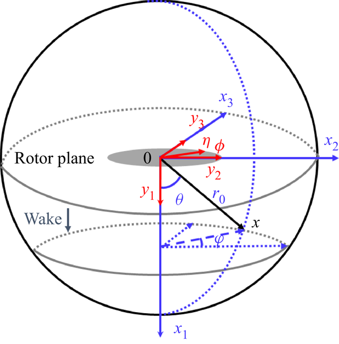
Figure 1. A schematic of the coordinate systems of the observer  $\boldsymbol {x}$ and source points $\boldsymbol {y}$.
There are several differences between (2.12) and the widely used Farassat formulation 1A (Farassat & Succi Reference Farassat and Succi1980). First, the convected wave equation accounts for the convection effect of oncoming flows. Second, the temporal derivative to the observer time  $t$ is kept in (2.12) to simplify the overall computation. Third, the term $1/|\partial g/\partial \tau |$ corresponding to the Doppler effect is explicitly expressed in the source coordinates, making it convenient to account for the impact of non-uniform rotational speed and blade vibration. A remark on the numerical implementation considering the challenges due to unsteady motions is given in Appendix A.
2.2. Estimating the source terms
Section 2.1 presents the mathematical framework of rotor noise computation with the effects of unsteady motions incorporated. To compute the rotor noise, we need to evaluate  $Q$ and $L_i$ at each surface point. An approach to computing the flow variables is to use high-fidelity numerical simulations, which, however, are too expensive for the parametric study of the influential factors. Nevertheless, in this work, CAA simulations will also be conducted for validation.
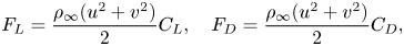
A reduced-order approach to computing the rotor noise source is the mean surface method (Hanson & Parzych Reference Hanson and Parzych1993; Zhong et al. Reference Zhong, Zhou, Fattah and Zhang2020). An illustration of the coordinate system and blade section elements is presented in figure 2. The rotor blade (the phase angle is  $\phi$) is divided into various small segments in the radial direction, and the width is $\mathrm {d}\eta$. At each section, we assume the flow is two-dimensional, and the axial and azimuthal velocities are $u$ and $v$, respectively. Here, $u$ contains the inflow projection and induced flow in the axial direction and $v$ contains inflow projection, blade rotation and induced flow in the tangential direction. Then, the term $Q\,\mathrm {d}S$ in (2.12) can be estimated as
 \begin{equation} Q\,\mathrm{d}S=\rho_\infty \boldsymbol{u}\boldsymbol{\cdot }\boldsymbol{n}\,\mathrm{d}S. \end{equation}
In the mean surface method (Hanson & Parzych Reference Hanson and Parzych1993; Zhong et al. Reference Zhong, Zhou, Fattah and Zhang2020), the projection of  $\boldsymbol {u}$ on the normal vector $\boldsymbol {n}$ is linked to the local pitch angle $\theta _c$ and thickness $h$ as
 \begin{equation} Q\,\mathrm{d}S = \rho_\infty[u\sin\theta_c + v\cos\theta_c]\,\mathrm{d}\eta\,\mathrm{d}h, \end{equation}
where  $\mathrm {d}h$ is the variation of blade thickness in the chord direction.
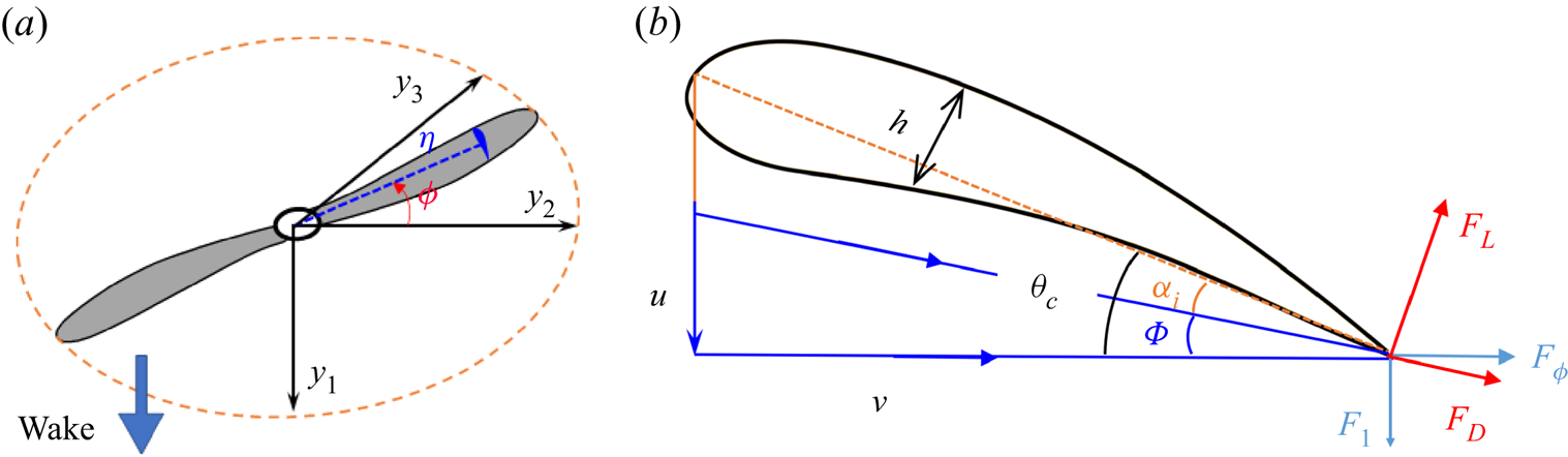
Figure 2. An illustration of the variables for rotor noise source estimation. (a) Rotor coordinate system. (b) Variables on a section.
The aerodynamic loading acting on the blade surface will contribute to  $L_i$. For each section shown in figure 2, the forces per unit area in the axial and azimuthal directions are denoted as $F_1$ and $F_\phi$, respectively. The projections in the $\boldsymbol {y}$-coordinate are
 \begin{equation} L_1 ={-}F_1,\quad L_2 = {\zeta} F_\phi\sin\phi, \quad L_3 ={-} {\zeta} F_\phi\cos\phi, \end{equation}
where  ${\zeta }=1$ if the blade rotates in the anti-clockwise direction and ${\zeta }=-1$ otherwise. As shown in figure 2, the angle of total velocity with the rotation plane is denoted as $\varPhi$. Then the equivalent angle of attack $\alpha _i$ is computed as
 \begin{equation} \alpha_i = \theta_c - \varPhi. \end{equation}
Under the assumption that the sectional flow is two-dimensional, at the given  $\alpha _i$ and Reynolds number (based on the velocity and chord length), the lift and drag are computed as
 \begin{equation} F_L = \dfrac{\rho_\infty(u^2 + v^2)}{2} C_L, \quad F_D = \dfrac{\rho_\infty(u^2 + v^2)}{2} C_D, \end{equation}
where  $C_L$ and $C_D$ are the lift and drag coefficients. As shown in figure 2(b), $F_L$ and $F_D$ are perpendicular and parallel to the total velocity that has an angle of $\varPhi$ to the rotational plane. Then the force projections in the axial and azimuthal directions are
 \begin{align} F_1 = \dfrac{\rho_\infty(u^2 + v^2)}{2}(C_D\sin\varPhi-C_L\cos\varPhi), \quad F_\phi = \dfrac{\rho_\infty(u^2 + v^2)}{2}(C_L\sin\varPhi + C_D\cos\varPhi), \end{align}
which are substituted to (2.18a–c) to estimate  $L_i$, and $L_i\mathrm {d}S$ is computed as
 \begin{equation} L_i\,\mathrm{d}S \approx L_ic\,\mathrm{d}\eta, \end{equation}
where  $c$ is the chord length.
2.3. Incorporating the effects of unsteady motions and uncertainty factors
For a parametric study of unsteady motions and uncertainty factors on rotor noise, we use a cost-effective method based on the blade element moment theory (BEMT) to obtain the aerodynamic variables for source modelling. At a given working state, the sectional flow velocity  $\boldsymbol {u}$, lift and drag coefficients $C_L$ and $C_D$ and therefore the sources based on using (2.17) and (2.22) can be computed. Therefore, the surface integrations in (2.12) are replaced by line integrations. This compact formulation is valid for slender surfaces such as rotors (Bernardini, Gennaretti & Testa Reference Bernardini, Gennaretti and Testa2016; Lopes Reference Lopes2017). The same approach was employed in our previous study of the frequency-domain formation of rotor noise computation (Zhong et al. Reference Zhong, Zhou, Fattah and Zhang2020).
However, it is still challenging to consider the unsteady aerodynamic effects in BEMT because of the possible random and complex motions. Fortunately, for practical problems, the amplitudes of these unsteadinesses are often small compared with the mean values. Therefore, we assume the lift coefficient  $C_L$ and drag coefficient $C_D$ of the sectional airfoil are the same as in ideal operations. A justification of this assumption is made in the next section using CAA. However, fluctuations in both $u$ and $v$ can still lead to perturbations in the source terms $Q$ and $L_i$. The term $|\partial g/\partial \tau |$ is also altered. In the future, the effects of unsteady velocity on aerodynamic properties (Van der Wall & Leishman Reference Van der Wall and Leishman1994) can also be considered in the model.
More specifically, in this work, we mainly focus on the rotor operations without oblique flow, i.e. the oncoming flow at the speed of  $u_\infty =|\boldsymbol {u}_\infty |$ is aligned with the rotor axis. The target rotational speed is $\varOmega _0$, and the chord length at each radial location (denoted as $\eta$) is $c_0$. To describe the unsteady motion, we denote the actual rotation speed as
 \begin{equation} \varOmega(\tau) = \varOmega_0 [1 +\varepsilon_0 + \varepsilon_1(\tau)], \end{equation}
where  $\varepsilon _0$ is a parameter describing the relative deviation of the actual rotation speed $\varOmega$ from the target value $\varOmega _0$, and $\varepsilon _1$ describes the temporal variations. In this case, the actual velocity in the tangential direction is
 \begin{equation} v(\tau) = \varOmega(\tau)\eta = \varOmega_0\eta[1 + \varepsilon_0 + \varepsilon_1(\tau)]. \end{equation}
Similarly, if the blade is vibrating, we introduce the parameter  $\varepsilon _2$ to quantify the corresponding velocity fluctuation in the axial direction as
 \begin{equation} u(\tau) = u_0 + \varepsilon_2(\tau)v_0 = u_\infty + u_* + \varOmega_0\eta\varepsilon_2(\tau), \end{equation}
where  $u_*$ is the induced velocity by the rotor, and it can be computed by using BEMT. As for the geometry asymmetry, in this work, we focus on the possible chord variation
 \begin{equation} c(\eta) = c_0(\eta)[1 + \varepsilon_3(\eta)], \quad \Rightarrow \quad \mathrm{d}S = [1 + \varepsilon_3]c_0\,\mathrm{d}\eta. \end{equation}
The parameter  $\varepsilon _3$ is time invariant but may vary with the radial location. In practice, other factors such as pitch angle variation and section geometry difference can also cause asymmetry. However, the description and following analysis will be similar and are, therefore, not repeated. In this work, we assume the amplitudes of these unsteady motions and uncertainty factors are small, i.e.
 \begin{equation} |\varepsilon_0|, \ |\varepsilon_1|, \ |\varepsilon_2|, \ |\varepsilon_3| \ll 1. \end{equation}
3. Influences on the aeroacoustics of an isolated rotor
This section will present the parametric study of influences of various unsteadiness and uncertainty factors on the rotor noise. Before that, justification, verification and validation of the noise computation model in § 2 will be presented.
3.1. Verification of the noise computation model implementation
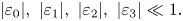
First, we will verify the implementation of the noise computation model by comparing results with experimental measurements in an anechoic chamber (Yi et al. Reference Yi, Zhou, Fang, Guo, Zhong, Zhang, Huang, Zhou and Chen2021; Wu et al. Reference Wu, Chen, Fattah, Fang, Zhong and Zhang2020). The two-bladed rotors APC  $9\times 5$ (with the tip radius of $r_{tip}=11.43$ cm) and APC $11\times 5$ (with the tip radius of $r_{tip}=13.97$ cm) are investigated. The sectional profile of both blades is close to the NACA4412 airfoil, and the chord and pitch angle distributions in the radial directions are shown in figure 3. Ten microphones at a distance of $1.5$ m from the rotor centres are used, and the equivalent observer angle ranges from $\theta =55^\circ$ to $118^\circ$. In experiments, both rotors are operated at various revolutions per second (RPS). However, there are inevitable deviations and fluctuations in the rotation speeds, which are measured using an optical encoder, and the results are shown in figure 4. The averaged values are kept relatively stable when the speeds are increased after a short time interval. The sampling frequency for RPS measurement is $50$ Hz. The unsteadiness quantified by $\varepsilon _1 = (\mathrm {RPS} - {\mathrm {RPS}_0})/{\mathrm {RPS}_0}$, where $\mathrm {RPS}_0$ is the target/nominal rotation speed, is shown in figure 4(b), and the amplitude is within $\pm 0.01$.
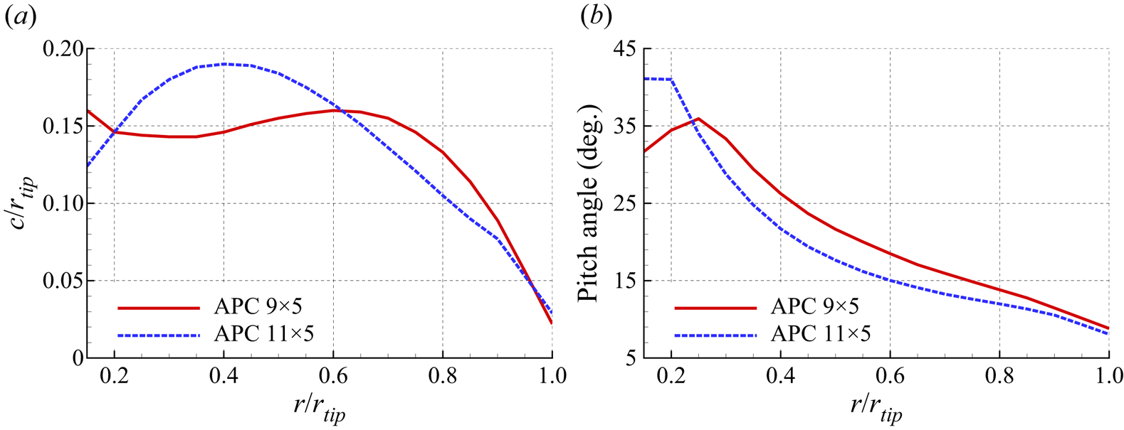
Figure 3. Chord and pitch angle distributions of the two tested APC blades in the radial directions. (a) Chord distribution, (b) pitch angle distribution.
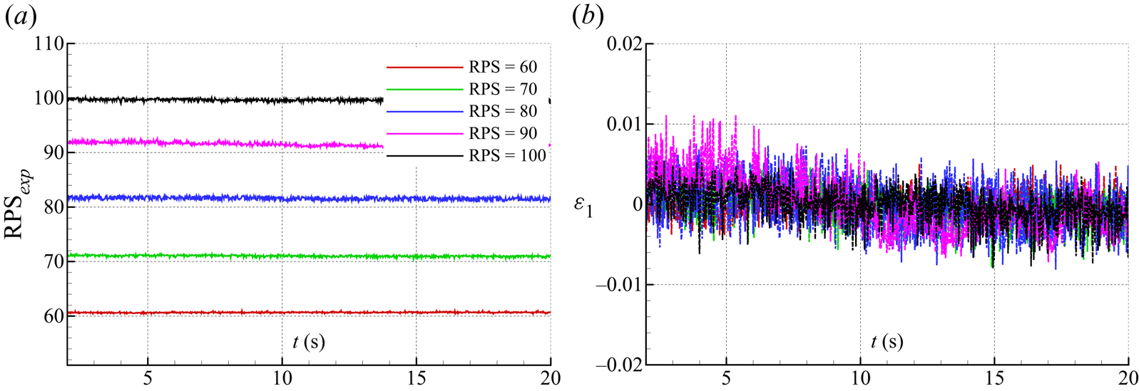
Figure 4. Examples of the measured RPS of a rotor at different target rotation speeds. (a) Measured RPS, (b) relative error  $\varepsilon _1$.
In the rotor noise prediction model, constant RPS with the averaged values  $\mathrm {RPS}_0$ shown in figure 4 and fluctuated RPS are employed as input. For the fluctuated RPS, random fluctuations with the amplitude of $0.01\mathrm {RPS}_0$ are added to the averaged value at each time step. In the experiments, it is found that the sound pressure level (SPL) at the blade passing frequency (BPF), which is equal to $2\times \mathrm {RPS}_0$ for the two-bladed rotors, is often insensitive to the unsteady fluctuations. To this end, in figure 5, we compare the predicted SPL result at different observers with the experimental measurements, showing a close agreement. However, the sampling frequency of the RPS measurements in experiments is only 50 Hz, and variations at high rates are not captured. Therefore, predictions using the fluctuated RPS cannot reproduce the impact of rotation speed unsteadiness on the sound radiation at high frequency. Nevertheless, the close results at the BPF by different approaches, i.e. experiments, constant RPS and fluctuated RPS predictions, suggested the implementation of the prediction model outlined in § 2 is well verified.
Figure 5. Comparisons of the predicted SPL of the tonal noise at BPF with experiments; (a) APC  $9\times 5$, (b) APC $11\times 5$.
3.2. Validation using CAA
We also conduct CAA simulations for the APC 9 $\times$5 rotor with unsteady rotation speeds to validate the prediction model and justify some assumptions taken in § 2.3. The acoustic preserved artificial compressibility equations suitable for low Mach number aeroacoustic simulations were implemented using an open-source library (Jiang & Zhang Reference Jiang and Zhang2022). The time marching is realised using a low-dissipation and low-dispersion Runge–Kutta scheme (Hu, Hussaini & Manthey Reference Hu, Hussaini and Manthey1996). In the near field, locally orthogonal grids are employed to resolve flow evolution and noise generation. The overall mesh consists of around $15\times 10^6$ cells in the computational domain. The accuracy of the CAA solver for rotor noise simulation has been validated by comparing the predictions with experimental test results (Jiang & Zhang Reference Jiang and Zhang2022; Jiang et al. Reference Jiang, Wu, Chen, Zhou, Zhong, Zhang, Zhou and Chen2022). In the study, $\mathrm {RPS}_0=90$ and the actual RPS is configured as
 \begin{equation} \mathrm{RPS}=\mathrm{RPS}_0[1 + \varepsilon_1\cos(2{\rm \pi} \tilde{f} t)],\quad \mathrm{where}\ \varepsilon_1=0.01,\ \tilde{f}=10\times\mathrm{RPS}_0. \end{equation}
The unsteady thrust predicted by the CAA simulation is shown in figure 6(a). The time-averaged thrust is  $T_0\approx 2.62$ N, which is close to the steady rotor simulation result using CAA. The thrust prediction by BEMT is approximately $2.6$ N. In § 2.3, we assume that $C_L$ and $C_D$ are unchanged in the presence of the unsteady motion, which should be examined using the CAA results. For simplicity, we denote the thrust coefficient for the steady rotor as $C_0$, i.e. $T_0=C_0\varOmega _0^2$, where $\varOmega _0=2{\rm \pi} \times \mathrm {RPS}_0$. The thrust coefficient of the unsteady rotor is denoted as $C$ such that
 \begin{equation} T(t) = C\varOmega^2 = C\varOmega_0^2[1+\varepsilon_1\cos(2{\rm \pi} \tilde{f}t)]^2 \approx T_0 \frac{C}{C_0} [1+ 2\varepsilon_1 \cos(2{\rm \pi} \tilde{f}t)], \end{equation}
where  $\varOmega =2{\rm \pi} \times \mathrm {RPS}$. Then, we perform Fourier transform of $T(t)$ (normalised by $T_0$) obtained by CAA, and the result is shown in figure 6(b). At $f/\mathrm {RPS}_0=10$, the amplitude of the normalised spectrum is close to $2\varepsilon _1$, as indicated by the red dot, suggesting that $C/C_0\approx 1$, i.e. the thrust coefficient remains unchanged. Therefore, the assumption of constant $C_L$ and $C_D$ employed in the prediction model is indirectly justified.
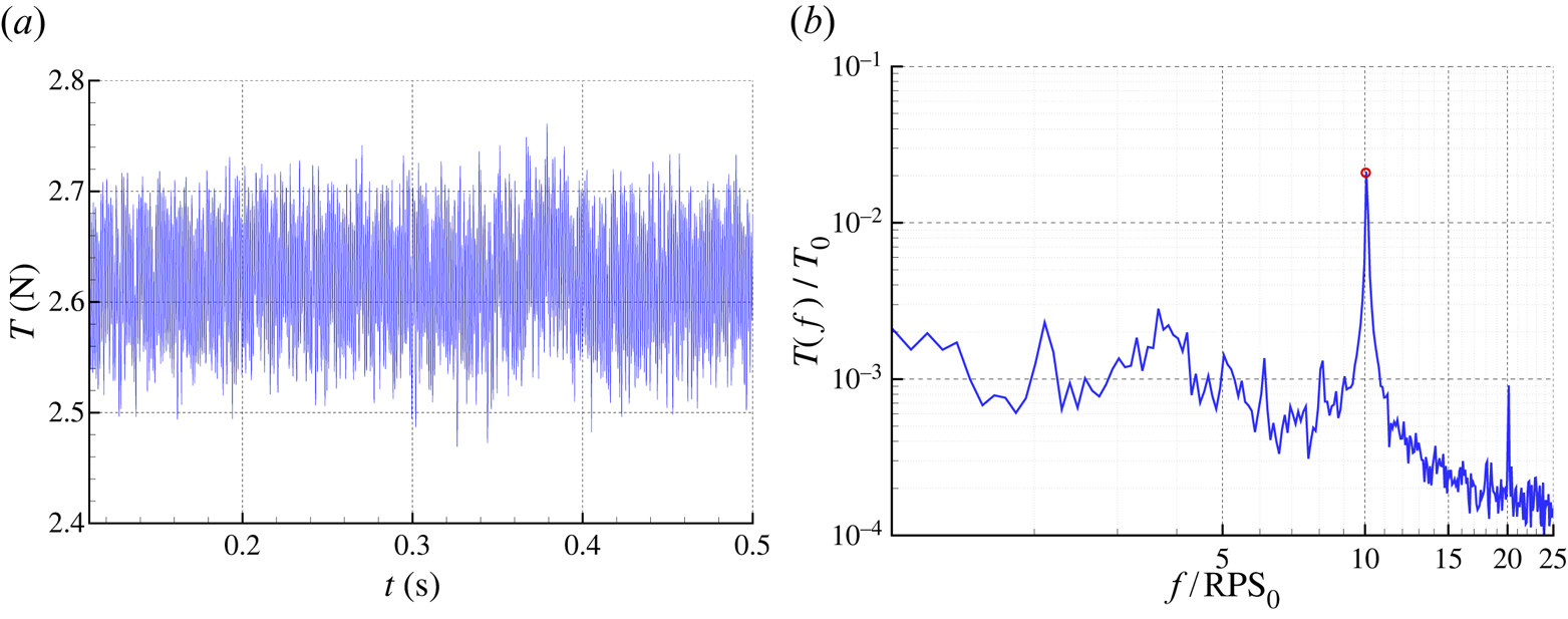
Figure 6. The computed time signal and spectrum of the rotor with fluctuated rotation speed using high-fidelity CAA simulation. For this case,  $\mathrm {RPS}_0=90$. (a) Thrust signal, (b) thrust spectrum (scaled by $T_0$).
In the numerical simulation, sound pressures at different observer points are also obtained and compared with the prediction results. Figure 7 shows the comparisons of noise spectra at  $r_o=0.2$ m and $0.4$ m. Both observers have the same observer angle of $\theta =90^\circ$, but the spectra are quite different because they are located in the near field. At BPF and its harmonics, the predicted SPLs are close to the high-fidelity CAA simulation. The computation times for the prediction model and high-fidelity CAA are a few seconds and more than 24 h, respectively. However, the broadband noise, mainly caused by the turbulence interaction at both the leading edge and trailing edge of the blades, is not contained in the prediction model.
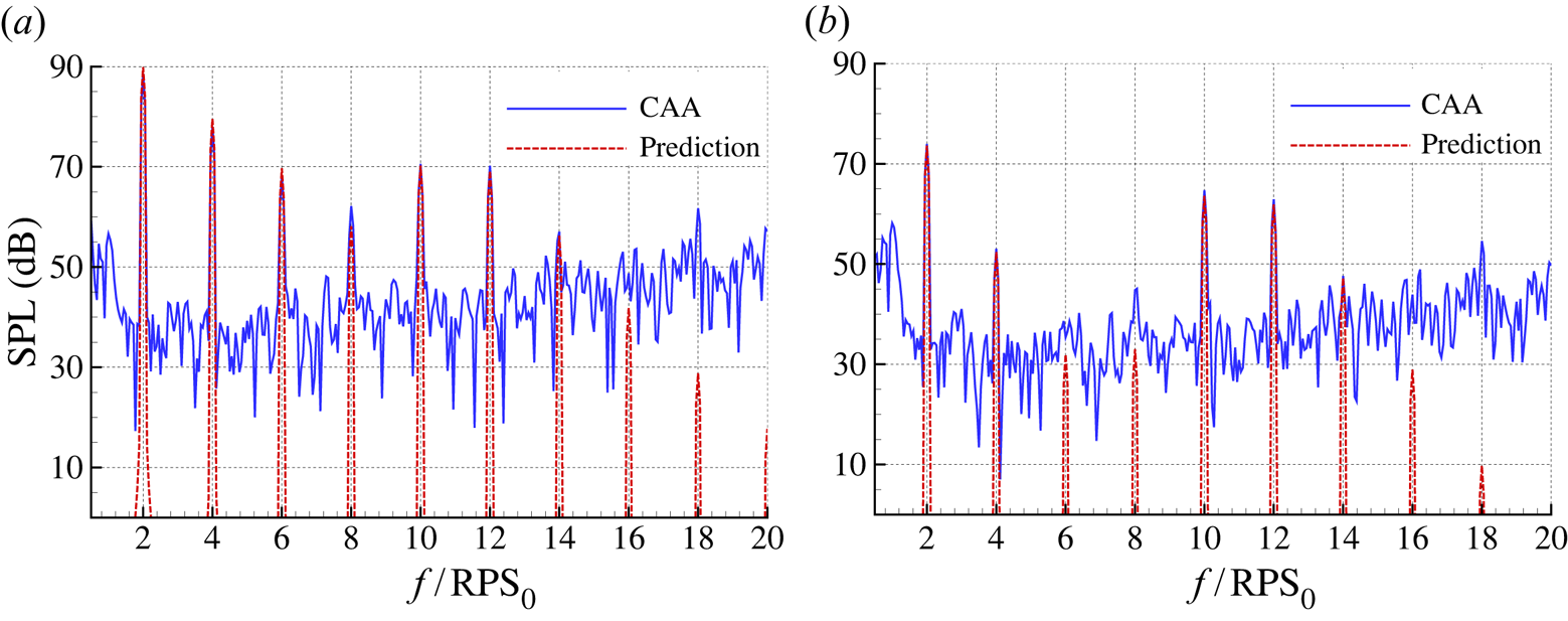
Figure 7. Comparisons of the predicted SPL spectra with high-fidelity CAA simulations at  $\theta =90^\circ$ and different observer distances $r_o$. For this case, $\mathrm {RPS}_0=90$; (a) $r_o=0.2$ m, (b) $r_o=0.4$ m.
3.3. Influence of rotation speed variation
In the following, we will conduct a parametric study of the unsteady motion and uncertainty factors based on the two-bladed rotor APC  $9\times 5$, i.e. the blade number $B=2$, in the hover state. The target rotation speed is $\mathrm {RPS}_0=100$. The observer distance is set as $r_o=1.5\,\mathrm {m}\approx 13r_{tip}$, where $r_{tip}$ is the rotor radius.
In this section, we study the influence of rotation speed variation using the proposed time-domain formulations in § 2. The additional source strengths of  $\Delta Q$, $\Delta F_L$ and $\Delta F_D$ are linearly dependent on the parameters $\varepsilon _0$ and $\varepsilon _1$. However, the variation of $\varepsilon _1$ also influences the estimated retarded time and the associated time derivatives, affecting the sound in a wide frequency range. In this section, we rewrite the relative difference between $\varOmega _0$ and $\varOmega$ defined in (2.23) as
 \begin{equation} \varepsilon_0 + \varepsilon_1(\tau) = \varepsilon_0 + \sum A_n\cos(2{\rm \pi} f_n \tau+\gamma_n) + \varepsilon_1^*(\tau), \end{equation}
where  $\varepsilon _0$ means the static deviation, and $\varepsilon _1$ and $\varepsilon _1^*$ describe the periodic and random fluctuations.
3.3.1. Static deviation of rotation speed
If the uncertainty factor in the rotation speed only contains the static deviation  $\varepsilon _0$, the actual rotation angular frequency $\varOmega$ has a deviation from the target value of $\varOmega _0$. One consequence is that the BPF has a variation of $\varepsilon _0\times \mathrm {BPF}$. The effect is shown in figure 8(a), where the frequency of each harmonic of BPF varies with $\varepsilon _0$ linearly. Moreover, in this case, the noise is dominated by the tonal noise at the BPF. The varied rotation speed can alter the strength of noise emission, and the acoustic scaling law (Zhong et al. Reference Zhong, Zhou, Fattah and Zhang2020) suggests the sound pressure amplitudes have a dependence of $(\varOmega /\varOmega _0)^h$, i.e. the difference in the SPL is
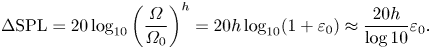 \begin{equation} \Delta\mathrm{SPL} = 20\log_{10}\left(\frac{\varOmega}{\varOmega_0}\right)^h = 20h \log_{10}(1+\varepsilon_0) \approx \frac{20h}{\log{10}}\varepsilon_0. \end{equation}
The coefficient  $h$ is dependent on the order of the BPF harmonics and observer angle (Zhong et al. Reference Zhong, Zhou, Fattah and Zhang2020). The dependence of the overall sound pressure level (OASPL) computed in the frequency range of 50–5000 Hz with $\varepsilon _0$ at different observers is shown in figure 8(b). At $\theta =90^\circ$, the coefficient is $h=B+2=4$ for the tone at BPF, which is a significant contribution to sound if the steady aerodynamic forces are considered. By contrast, at $\theta =30^\circ$ and $\theta =150^\circ$, the noise at BPF is less significant while the contributions by tones at higher frequencies, which have other dependencies on $\varOmega$, are increased, leading to different slopes. In the figure, the low noise levels at $-160$ dB, i.e. the sound pressure amplitudes tend to $0$, are presented, which, however, might be covered by other noise components in practice.
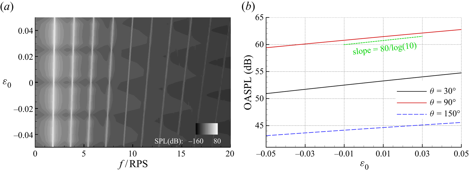
Figure 8. The influence of the static deviation of the rotational speed; (a) spectra, (b) OASPL.
For a single rotor, when  $\varepsilon _0$ is small, e.g. $|\varepsilon _0|<0.01$, the influence on the SPL is negligible. The difference in the peak location is distinguishable due to the finite frequency resolution. However, it does not mean that the RPS deviation effect is unimportant. For example, in dual rotor applications, the difference in the rotation speed can lead to a varying phase difference between the rotating blades, altering the interference effect of the sound waves. The effect will be investigated in § 4.
3.3.2. Periodic fluctuation of rotation speed
In this section, we consider cases such that the rotational speed fluctuation is periodic, i.e. the influence of sinusoidal terms in (3.3) is studied. The frequency of the RPS fluctuation is  $f_n$, and it is not necessarily a harmonic of $\mathrm {BPF}$ as in the frequency-domain solver (Hanson & Parzych Reference Hanson and Parzych1993; Zhong et al. Reference Zhong, Zhou, Fattah and Zhang2020).
Figure 9 shows the acoustic spectra with  $f_n=500$ Hz (i.e. $5\times \mathrm {RPS}_0$) at $\theta =30^\circ$ and $90^\circ$, respectively. When $A_n=0$, which means the rotation has a constant speed, tonal noise is produced at the $\mathrm {BPF}=2\times \mathrm {RPS}_0$ and its harmonics. However, the SPL is rapidly reduced with the increase of harmonic number. For example, the SPL at $2\times \mathrm {BPF}$ is lower than that at $\mathrm {BPF}$ by approximately 40 dB. By contrast, if there is a slight variation in the rotation speed, e.g. for cases with $A_n=1\times 10^{-3}$, $2\times 10^{-3}$ and $4\times 10^{-3}$, additional tonal noise is produced at $f_n$, and the SPL is comparable to that at BPF. Multiple peaks are also found at other frequencies of $f_n + k\times \mathrm {RPS}_0$, where $k$ is an integer. As shown in the zoomed regions in figure 9, at $f=f_n$, the SPL increases by approximately $6$ dB when $A_n$ is doubled, suggesting that the magnitude of produced sound is proportional to the periodic fluctuation amplitude $A_n$. It should be emphasised that the extra tones at the harmonics of $\mathrm {RPS}_0$ cannot be captured by the frequency-domain method (Hanson & Parzych Reference Hanson and Parzych1993; Zhong et al. Reference Zhong, Zhou, Fattah and Zhang2020).
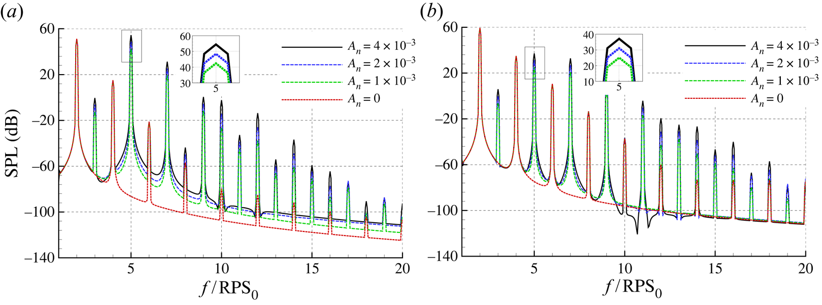
Figure 9. Computed rotor noise spectra at different observers if there are periodic fluctuations in the rotation speed. The frequency of periodic fluctuation is  $f_n=500$ Hz; (a) $\theta =30^\circ$, (b) $\theta =90^\circ$.
To further consider how the periodic unsteady motion affects the additional tonal noise components, we investigate the two close frequencies of  $f_n=1200$ Hz and $1230$ Hz. The computed noise spectra at $\theta =90^\circ$ are shown in figure 10. When $f_n=1200$ Hz, which is an integer multiple of the BPF, the noise peaks in the high-frequency range only appear at the harmonics of the BPF. By contrast, as shown in figure 10(b), when $f_n=1230$ Hz, amplitudes of the tonal noise at the harmonics of BPF are unchanged. There are significant tones at $(12.3+2k)\times \mathrm {RPS}_0$, where $k$ is an integer. Also, the amplitudes of those tones are close to those at $(12+2k)\times \mathrm {RPS}_0$ in figure 10(a). There are several slight peaks with a difference of $\pm 0.3\times \mathrm {RPS}_0$ from the main peaks. The results suggest that the periodic motions can produce significant tones related to both $f_n$, the frequency of the RPS fluctuation, and the mean rotation speed $\mathrm {RPS}_0$.
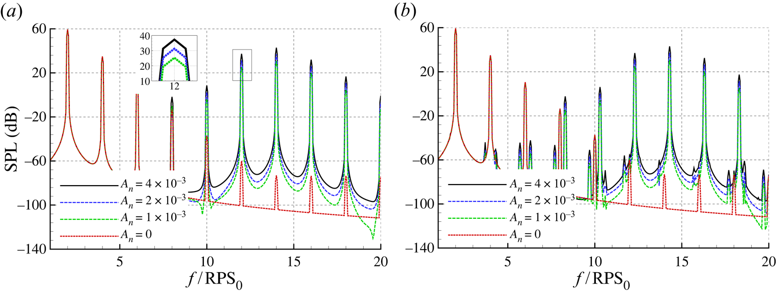
Figure 10. Computed spectra of the rotor noise at  $\theta =90^\circ$. There are periodic fluctuations with different $f_n$ in the rotation speed; (a) $f_n=1200$ Hz, (b) $f_n=1230$ Hz.
To better understand the dependence of noise features on the frequency of the periodic motion, we compute the sound radiation with the parameter  $f_n$ ranging from $0$ to $1600$ Hz. The mean rotation speed is $\mathrm {RPS}_0=100$. The corresponding acoustic spectra are computed, and the results at $\theta =30^\circ$ and $90^\circ$ are shown in figure 11. For different $f_n$, the peak values are always high at the BPF and its harmonics, which are likely contributed to by the mean rotation speed. Besides, there are high levels of sound at the frequency of $f=f_n$, and there are relatively low but discernible peaks at the alternative frequencies of $f=f_n \pm l\times \mathrm {BPF}$, where $l$ is an integer. In figure 10(b), there are also peaks at the frequencies that seem to be the combination of the BPF and $f_n$, although the levels are relatively low. Figure 11 shows that there is a complex dependence of the observed peak locations on $f_n$, especially when $f_n$ is high. By contrast, at low perturbation frequency, e.g. $f_n<2\times \mathrm {RPS}_0$, the periodic motion only produces several peaks at low frequencies, and the influence on the tonal noise at high frequencies is relatively unimportant. At $\theta =90^\circ$, clear tones are produced at high $f_n$. The results suggest that the periodic motion can equivalently produce an additional sound source at $f_n$, which is then modulated by the rotational motion of the blade at $\mathrm {RPS}_0$.
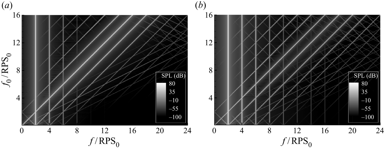
Figure 11. Computed spectra of a two-bladed rotor with periodic fluctuation in RPS. The amplitude of the periodic fluctuations is  $A_n=2\times 10^{-3}$, and $f_n$ ranges from $0$ to $1600$ Hz; (a) $\theta =30^\circ$, (b) $\theta =90^\circ$.
The investigation of the acoustic spectra suggested that the periodic fluctuation of the rotation speed can produce additional tonal noise. The locations of the peaks are sensitive to  $f_n$ and are related to $\mathrm {RPS}_0$. Figure 9 shows that, if additional peaks are produced due to the periodic motion, the amplitudes of the sound pressure are likely proportional to the amplitude $A_n$. However, the noise due to the overall aerodynamic force due to the rotation is also significant, especially at BPF. To this end, in this work, we consider the extra acoustic energy estimated by integrating the sound power from $50$ to $5000$ Hz, due to the unsteady periodic fluctuation. The dependence of the extra sound energy on $f_n$ and $A_n^2$ is shown in figure 12. In the results, $A_n^2$ indicates the amplitude of the equivalent sound source that is likely proportional to the amplitude of the unsteady fluctuation. The values are multiplied by $100$ for convenience. When $f_n$ is relatively high, e.g. $f_n>9\times \mathrm {RPS}_0$, a relatively even increase of $\Delta E$ with $A_n^2$ is achieved, suggesting that the strength of the extra sound pressure is dependent on $A_n$ linearly. By contrast, at low $f_n$, there is a lower increase of $\Delta E$ with the same $A_n^2$. Moreover, the amplitudes of the extra acoustic energy at $\theta =90^\circ$ are much lower than that at $\theta =30^\circ$.
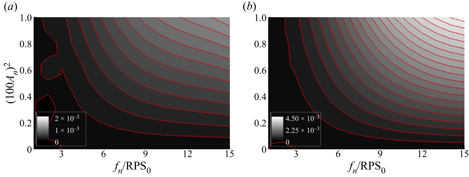
Figure 12. The dependence of additional acoustic energy  $\Delta E$ on $f_n$ and $A_n$ of the periodically fluctuated rotation speed at different observer angles; (a) $\theta =30^\circ$, (b) $\theta =90^\circ$.
The acoustic directivity of the SPL at BPF, and the OASPL (calculated from  $50$ to $5000$ Hz) with $f_n=500$ Hz and $1200$ Hz, respectively, is computed. The observer angles range from $\theta =30^\circ$ to $150^\circ$, and the amplitudes of $A_n=1\times 10^{-3}$, $2\times 10^{-3}$ and $4\times 10^{-3}$ are considered. The results are shown in figure 13. At both frequencies, little difference is found at $\theta =90^\circ$ for different $A_n$. The reason is that the original noise level at the BPF is relatively high; meanwhile, the extra acoustic energy due to the unsteady factor is relatively low, slightly changing the noise level. By contrast, the unsteady effect is more profound in the upstream and downstream directions, while the original levels at the corresponding locations are low, leading to a significant increase.
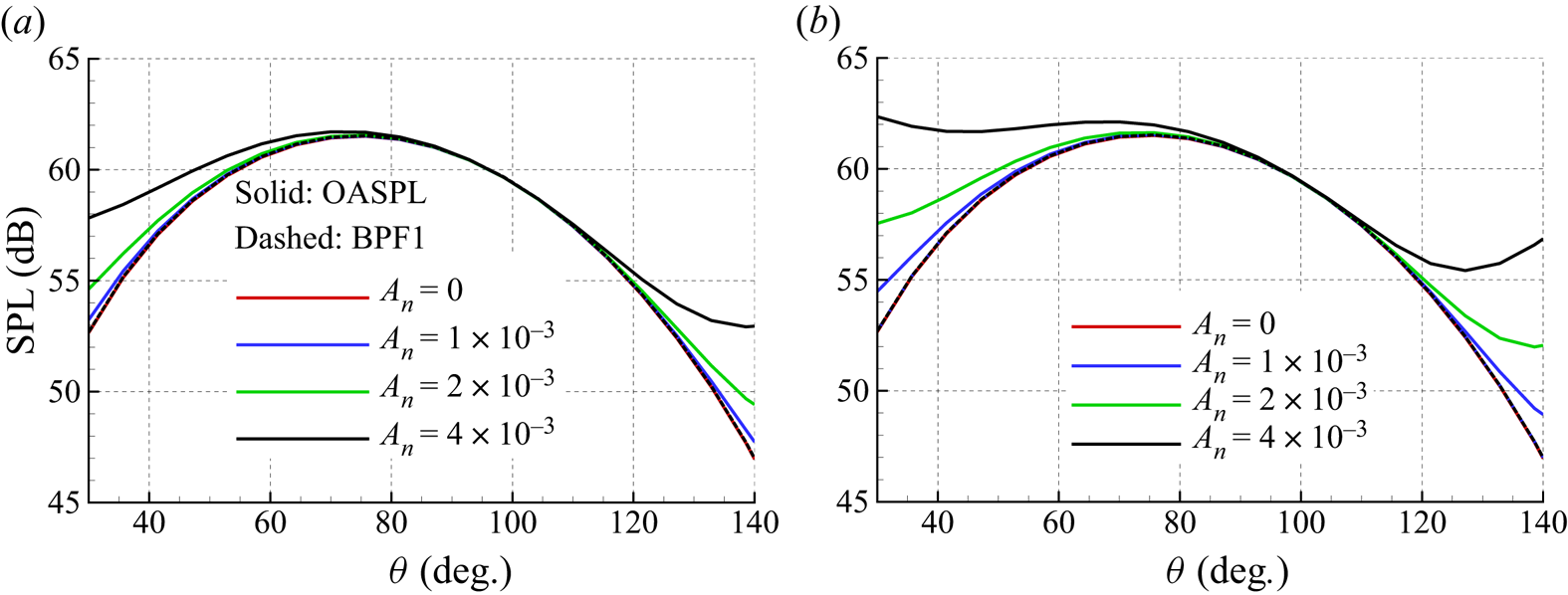
Figure 13. A comparison of directivities with rotation speed variations at different  $f_n$; (a) $f_n=500$ Hz, (b) $f_n=1200$ Hz.
3.3.3. Random fluctuation of rotation speed
This section studies the influence of random fluctuations in the actual  $\mathrm {RPS}$, described by the term $\varepsilon _1^*$ in (3.3). In experiments, determining the property of $\varepsilon _1^*$ is difficult as a high sampling frequency is needed to obtain the instantaneous rotation speed. Therefore, we assume that the inevitable random fluctuations (see figure 4) have power spectral density (PSD) with Gaussian distributions
 \begin{equation} {E}_1^*(f)=A_G\exp[-\varLambda_A(f-f_c)^2], \end{equation}
where  $f$ is the frequency, $A_G$ is the amplitude and $\varLambda _A$ and $f_c$ control the shape of the spectrum. In this work, $\varLambda _A=10^{-4}$ is studied without loss of generality. Figure 14(a) shows the two spectra with $f_c=500$ Hz and $f_c=1000$ Hz with $A_G=5\times 10^{-8}$. The spectra in the frequency domain are realised as randomly varying time signals $\varepsilon _1^*(t)$ shown in figure 14(b), based on which we recomputed the PSD, and the results reproduce the target spectra satisfactorily, as indicated by the dots in figure 14(a). With the time signals of $\varepsilon _1^*(t)$, we can compute the corresponding fluctuations in RPS. The fluctuating rotational speed is within $1\,\%$ of $\mathrm {RPS}_0$.
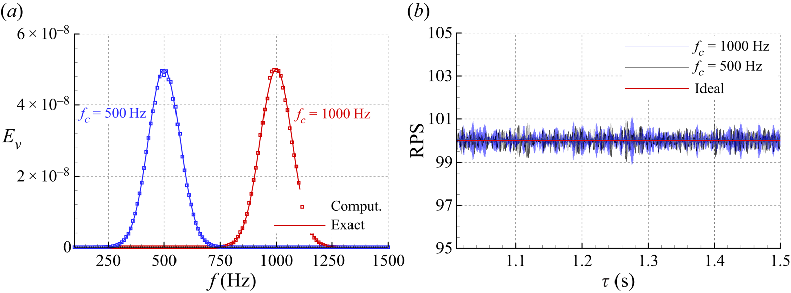
Figure 14. The spectra of the random fluctuations denoted by  $\varepsilon _1^*$ in the rotation speed and the synthesised time signals. (a) Spectra, (b) time signals.
Using the formulations outlined in § 2, we are able to compute the noise spectra with randomly fluctuated  $\mathrm {RPS}$. Figure 15 shows the results with $A_G$ ranging from $0.5\times 10^{-8}$ to $5\times 10^{-8}$. The observer angles are $\theta =30^\circ$ and $90^\circ$, and the results are compared with those with steady rotational speed (red dashed curves). The random fluctuations can lead to broadband-type noise features, while the tonal noise at BPF is slightly altered. The noise level due to the RPS fluctuation is much higher than the tonal noise peaks in a wide frequency range. At $\theta =90^\circ$, the tonal noise at $2\times \mathrm {BPF}$ is relatively high, and values are not altered by the random RPS fluctuations either. Furthermore, there are maximum values of a bump-shaped spectrum around $f_c=500$ Hz, relating to the PSD of $\varepsilon _1^*$. However, the bump shapes are observer angle dependent.
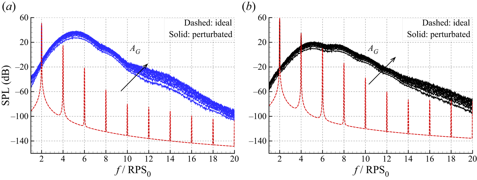
Figure 15. Computed noise spectra with random fluctuations in RPS. The fluctuations have Gaussian distributions, and  $f_c=500$ Hz and $A_G$ ranges from $0.5\times 10^{-8}$ to $5\times 10^{-8}$; (a) $\theta =30^\circ$, (b) $\theta =90^\circ$.
As indicated by arrows in figure 15, the levels of the humps increase with  $A_G$. In this work, we extract the broadband noise spectra linked to the randomly perturbed RPS by using a robust locally weighted regression method (Cleveland Reference Cleveland1979). Moreover, the results due to different $A_G$ are scaled to that of $A_{G0}=0.5\times 10^{-8}$, i.e. we define a new variable of $\mathrm {SPL}^* = \mathrm {SPL} - 10\log _{10}{(A_G/A_{G0})}$, and the results are shown in figure 16. The humped peaks are collapsed around $f_c=500$ Hz and $1000$ Hz, respectively, suggesting the strengths of the equivalent broadband noise sources are proportional to $A_G$. In addition, the results are close for $\theta =30^\circ$ and $150^\circ$, and they are higher than that at $\theta =90^\circ$.
Figure 16. Computed equivalent broadband noise spectra with different random fluctuations in RPS. The SPL is scaled by  $B_G$, the amplitude of the random fluctuations; (a) $f_c=500$ Hz, (b) $f_c=1000$ Hz.
3.4. Influence of blade vibration
This section investigates the influence of blade vibration in the axial direction. Equation (2.25) introduces the parameter  $\varepsilon _2(t)$ for quantification, which, similarly, can be decomposed into the periodic motion and random fluctuation, i.e.
 \begin{equation} \varepsilon_2(\tau) = \sum B_n\cos(2{\rm \pi} f_n \tau + \varphi_n) + \varepsilon_2^*(\tau), \end{equation}
where  $B_n$ and $f_n$ are the amplitude and frequency of the periodic motion, respectively, and $\varepsilon _2^*$ corresponds to the possible random vibration.
First, the influence of periodic vibrations with  $f_n=100$ Hz and $1000$ Hz on rotor noise is studied. For both cases, the vibration amplitude is assumed as $B_n=2\times 10^{-3}$, and the computed spectra results are shown in figure 17. At $\theta =30^\circ$, for each periodic frequency $f_n$, peaks are found at $f_n + l\times \mathrm {BPF}$, where the $l$ values are integers. For example, when $f_n=100$ Hz (the green curves), extra peaks are found at $300\,{\rm Hz}, 500\,{\rm Hz}\text { and }700\,{\rm Hz}, \ldots$, with decreasing amplitudes. Similarly, when $f_n=1000$ Hz (the black curves), levels of the tonal noise at $800$ Hz, $1000$ Hz, $1200$ Hz and $1400$ Hz are significantly increased. However, at $\theta =90^\circ$, the noise spectra are little affected, being close to that of the steady blade. The results suggest that the blade variation can hardly affect the tonal noise on the rotational plane because the blade vibrations can cause pulsating motions in the axial direction, resulting in an equivalent acoustic dipole. This conclusion is also applicable to other $f_n$. Figure 18 shows the spectra at $\theta =30^\circ$ and $\theta =90^\circ$ with $f_n$ ranging from $0$ to $1600$ Hz. Clear tones at BPF and its harmonics are found at both observer angles. Moreover, at $\theta =30^\circ$, there are also multiple parallel lines at $f = f_n + l\times \mathrm {BPF}$. At $\theta =90^\circ$, the tonal noise only occurs at the harmonics of BPF.
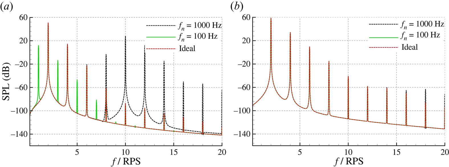
Figure 17. Computed noise spectra at different observers with periodic blade vibrations. Here,  $B_n=2\times 10^{-3}$ and $f_n=100$ Hz and $1000$ Hz are studied; (a) $\theta =30^\circ$, (b) $\theta =90^\circ$.
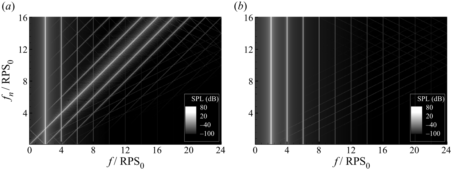
Figure 18. Computed noise spectra at different observer angles with periodic blade vibration. Cases with  $B_n=2\times 10^{-3}$, and $f_n$ ranges from $0$ to $1600$ Hz are studied; (a) $\theta =30^\circ$, (b) $\theta =90^\circ$.
The vibration can also be random, as described by  $\varepsilon _2^*$ in (3.6). In this case, we assume the PSD of the random fluctuation has a Gaussian distribution
 \begin{equation} {E}_2^*(f) = B_G\exp[-\varLambda_B(f-f_c)^2]. \end{equation}
In practical applications, time signals of  $\varepsilon _2^*(t)$ are realised by using the PSD in the frequency domain with $\varLambda _B=1\times 10^{-4}$, $f_c=500$ Hz and $B_G$ ranges from $0.5\times 10^{-8}$ to $5\times 10^{-8}$. A comparison of the resulting noise spectra at different observers is shown in figure 19. Again, the random vibrations do not alter the tonal noise components at the BPF harmonics (if discernible) in the spectra. Instead, they equivalently produce broadband-type spectra, and the noise level increases with $B_G$. At $\theta =30^\circ$, the broadband content is bumped shaped with the peak locations around $f=f_c$. At $\theta =90^\circ$, there are also broadband-shaped noise spectra, the amplitudes of which are much lower than that at $\theta =30^\circ$ (approximately $70$ dB). As a result, the peaks of the tonal noise are discernible at that observer angle. In this work, we also compute the OASPL (from $50$ to $5000$ Hz) of the equivalent components having a random vibration at different observer angles ranging from $\theta =30^\circ$ to $150^\circ$. The results for $f_c=500$ Hz and $f_c=1000$ Hz are shown in figure 20. High noise levels are found in the upstream and downstream directions due to the dipole property of the equivalent noise sources. The SPL data scaled by the amplitude as $\mathrm {SPL}^*=\mathrm {SPL}-10\log _{10}(B_G/B_{G0})$ with $B_{G0}=0.5\times 10^{-8}$ are shown in the insets in figure 20. The collapsed results suggest the strength of equivalent broadband noise is proportional to the amplitudes of the random vibration. Additionally, levels of the equivalent broadband noise increase with $f_c$.
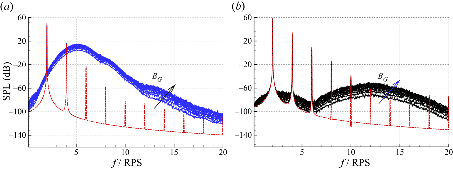
Figure 19. Computed noise spectra at different observers with random blade vibration with a Gaussian distribution. Here,  $f_c=500$ Hz and $B_G$ ranges from $0.5\times 10^{-8}$ to $5\times 10^{-8}$; (a) $\theta =30^\circ$, (b) $\theta =90^\circ$.
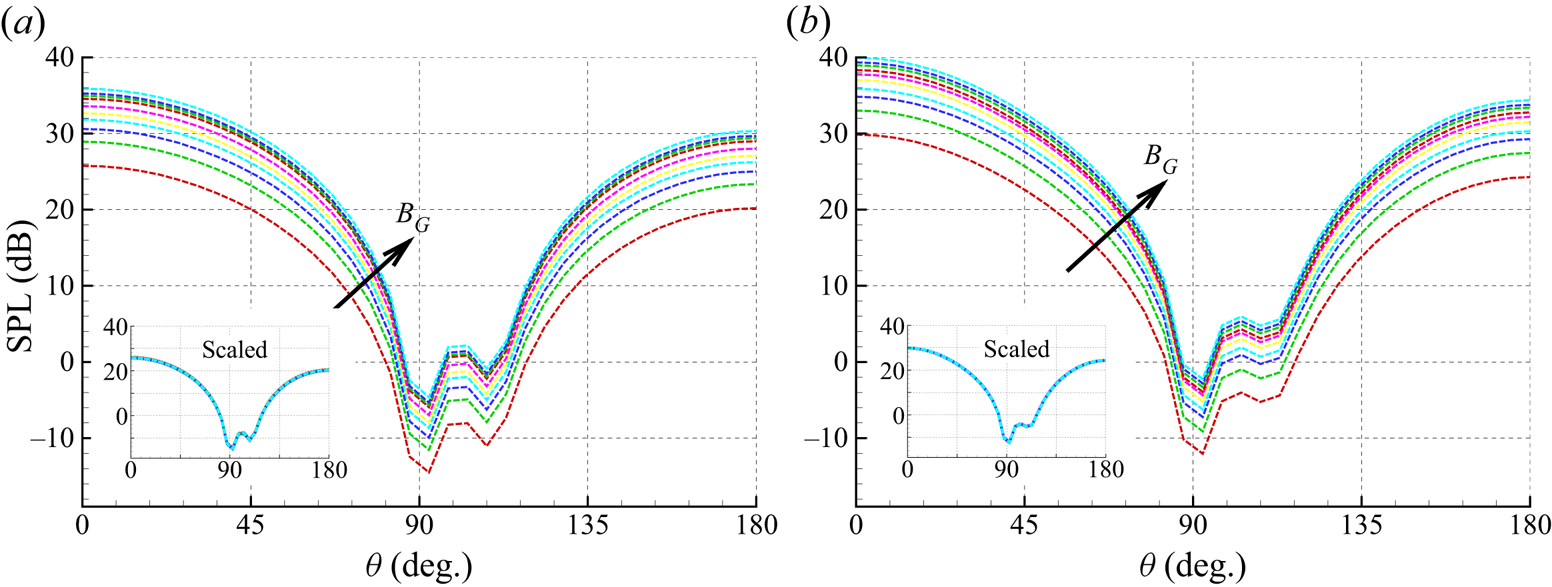
Figure 20. Computed directivity patterns of the equivalent broadband noise due to the random blade vibrations with  $f_c=500$ Hz and $1000$ Hz, respectively. Here, $B_G$ ranges from $0.5\times 10^{-8}$ to $5\times 10^{-8}$; (a) $f_c=500$ Hz, (b) $f_c=1000$ Hz.
3.5. Influence of geometry asymmetry
This section investigates the influence of geometry asymmetry on rotor noise emission. For the two-bladed rotor under investigation, we assume the chord of one blade is  $c=c_0(1+\varepsilon _3)$, while the other one remains $c_0$. In this work, small values of $\varepsilon _3=0.01$, $0.02$ and $0.04$ are investigated. First, we assume the rotor has a constant rotation speed, and the computed noise spectra at different observer angles are shown in figure 21. Compared with the symmetric rotor, which corresponds to $\varepsilon _3=0$, multiple extra peaks are found at $k\times \mathrm {RPS}_0+l\times \mathrm {BPF}$ with $k$ and $l$ as integers. Moreover, for those additional peaks, as indicated by the zoomed-in insets in figure 21, a difference of $6$ dB is found when $\varepsilon _3$ is doubled. Meanwhile, compared with the symmetric blade, the noise levels of the asymmetric blades at BPF harmonics are nearly unchanged.
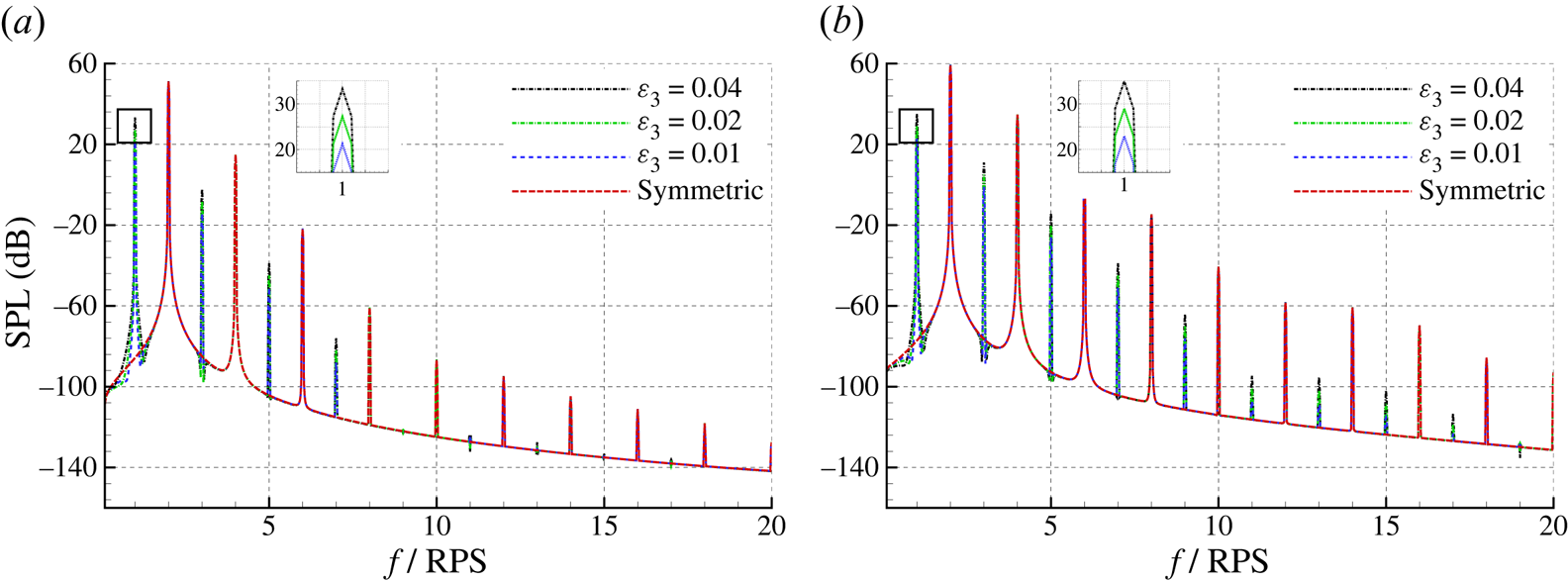
Figure 21. Computed noise spectra of asymmetric blades with constant  $\mathrm {RPS}=\mathrm {RPS}_0$; (a) $\theta =30^\circ$, (b) $\theta =90^\circ$.
Similarly, we can compute the noise spectra of the asymmetrical blades experiencing a periodic unsteady motion as quantified in (3.3). The frequency is  $f_n=1000$ Hz and the amplitude is $A_n=2\times 10^{-3}$. The results at different observer angles are shown in figure 22. Due to the periodic fluctuation of the rotation speed, the tonal noise around $10\times \mathrm {RPS}_0$ is increased, as investigated in § 3.3.2. Those peaks are not altered even though the blade geometries are asymmetric. Instead, there are additional tones between the peaks due to the periodically fluctuating rotation speed. The amplitudes of those tones (at $1\times \mathrm {RPS}_0, 3\times \mathrm {RPS}_0, 5\times \mathrm {RPS}_0, \ldots$) are increased by approximately $6$ dB when $\varepsilon _3$ is doubled. We can also compute the noise spectra of the asymmetric blade when the rotation speed has random fluctuations. The PSD of the random fluctuation is described in (3.3) with $A_G=5\times 10^{-8}$ and $f_c=500$ Hz. Again, as shown in figure 23, bump-type broadband noise is produced due to the fluctuated rotation speed, which overwhelms most of the tonal noise in the spectra. However, discernible peaks at $100$ Hz are found, and the amplitude increases with $\varepsilon _3$, while the noise level at BPF is unchanged.
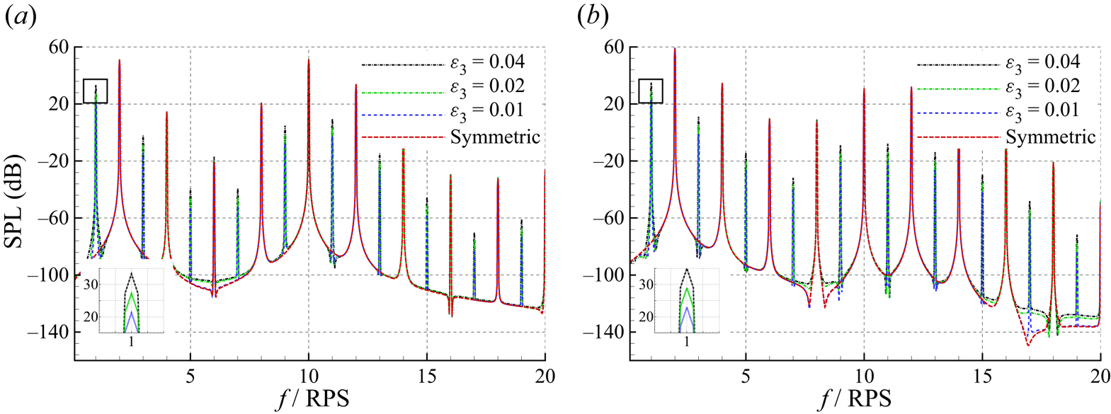
Figure 22. Computed noise spectra of asymmetric blades with periodically fluctuated RPS. The frequency of the periodic motion is  $f_n=1000$ Hz and the amplitude is $A_n=2\times 10^{-3}$; (a) $\theta =30^\circ$, (b) $\theta =90^\circ$.
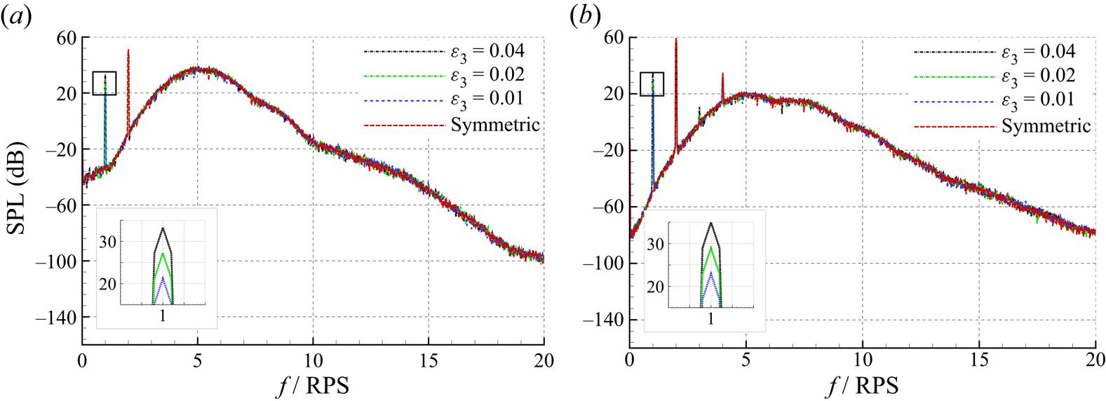
Figure 23. Computed noise spectra of asymmetric blades with random fluctuations in RPS ( $A_G=5\times 10^{-8}$ and $f_c=500$ Hz); (a) $\theta =30^\circ$, (b) $\theta =90^\circ$.
In this work, the asymmetry is described by introducing variations in the chord. A more generic configuration with spatially dependent  $\varepsilon _3$ can be considered as well. Technically, the effects of other uncertainties in pitch angle distribution can also be investigated using the same approach in this section. However, the blade asymmetry can cause mass imbalances in practice, resulting in structural vibration and altering the noise emission feature.
4. Influences on the aeroacoustics of dual rotors
In practical applications, a flying vehicle is often equipped with multiple rotors, and the rotation speed of each rotor is continuously adjusted for flight control. Studies on the aerodynamic noise features of multiple rotors have been conducted (Shukla & Komerath Reference Shukla and Komerath2018; Alvarez & Ning Reference Alvarez and Ning2020; Bernardini et al. Reference Bernardini, Centracchio, Gennaretti, Iemma, Pasquali, Poggi, Rossetti and Serafini2020; de Vries et al. Reference de Vries, van Arnhem, Sinnige, Vos and Veldhuis2021; Bu, Ma & Zhong Reference Bu, Ma and Zhong2022). However, the influence of the multi-rotor interaction on noise generation is still debated as contradictory conclusions were made in previous studies (Zhou et al. Reference Zhou, Ning, Li and Hu2017; Zhou & Fattah Reference Zhou and Fattah2017). The numerical studies by Lee & Lee (Reference Lee and Lee2020) showed a noise variation of up to  $20$ dB. By contrast, the experiments by Bu et al. (Reference Bu, Wu, Bertin, Fang and Zhong2021) suggested both aerodynamic forces and noise features are insensitive to the separation distances and initial configurations. The observations might be linked to the fact that the dual rotor aeroacoustics have been influenced by unsteady motions and uncertainty factors, which are studied in this section.
In the following study, we assume that the dual rotors, either co-rotating or counter-rotating, have identical geometry and are placed on the same plane. The separation distance of the centres is  $1.1D$, where $D$ is the rotor diameter. For this configuration, the effect of mutual interactions of the rotors on the aerodynamic force is regarded as insignificant (Bu et al. Reference Bu, Wu, Bertin, Fang and Zhong2021). Therefore, we assume the sound source generated aerodynamically by each rotor is the same as that of an isolated rotor.
4.1. Co-rotating dual rotors
Usually, the sound waves produced by the sources on the rotor blade surface experience different time delays as the source locations vary with the rotation. Therefore, for a dual rotor system, the difference in the initial phase angle  $\Delta \phi _0$ of the blades might significantly alter the noise feature. First, we study the co-rotating dual rotors at the constant rotation speed of $\mathrm {RPS}_0$ and $\Delta \phi _0=0^\circ$ and $90^\circ$. The resultant noise spectra at different observers quantified by the polar angle $\theta$ and azimuthal angle $\varphi$ (cf. the schematic in figure 1) are shown in figure 24. The results due to a single rotor are also included for comparison. The tonal noise components are only found at the harmonics of BPF, and the amplitudes decrease with frequency because there is no fluctuation in the rotation speed. At $\varphi =0^\circ$ (on the rotation plane), as shown in figure 24(a), the results at both $\Delta \phi _0=0^\circ$ and $90^\circ$ are close, and they are slightly higher than those of the single rotor. By contrast, because of the interference effect, the noise level of the $\Delta \phi _0=90^\circ$ case is lower than the $\Delta \phi _0=0^\circ$ case by $20$ dB at $\varphi =90^\circ$ (on the perpendicular plane). The results suggest that significant noise reduction at particular observers might be achieved via phase control.
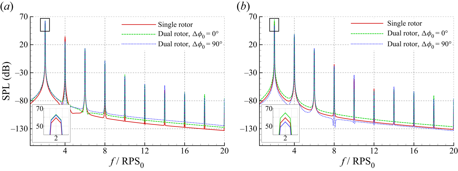
Figure 24. Computed sound spectra of two rotors with identical and constant rotation speeds. The observers are at (a)  $\theta =90^\circ$ and $\varphi =0^\circ$, (b) $\theta =90^\circ$ and $\varphi =90^\circ$.
Next, we will investigate the influence of rotational speed fluctuations on the sound interference. As described previously, for both  $\Delta \phi _0=0^\circ$ and $\Delta \phi _0=90^\circ$ cases, we assume the rotation speed has a periodic fluctuation at $f_n=1000$ Hz, and the amplitude is $A_n=10^{-3}$. A comparison of the computed noise spectra at different observer angles is shown in figure 25. Consequently, the tonal noise levels in the high-frequency range are increased due to periodic fluctuations. However, the impact of the mechanism of phase difference $\Delta \phi _0$ on the perceived noise is similar to that with constant rotation speed. At $\varphi =0^\circ$, the noise spectra of both configurations are close; at the observer angle of $\varphi =90^\circ$, a difference in SPL of up to $10$ dB is found between the $\Delta \phi _0=90^\circ$ and $\Delta \phi _0=0^\circ$ cases. Ideally, the temporal variation of the rotation speed can yield different phase angle differences of the sources and therefore affect the interference of sound waves. However, the accumulated phase difference remains small if the rotation speed fluctuation is periodic and the amplitude $A_n\ll 1$. More importantly, the frequency of the periodic fluctuation is high, making the actual variation in $\Delta \phi$ due to unsteady motion negligible. In other words, $\Delta \phi (t)\approx \Delta \phi _0$ and the effect of phase delay on the acoustic interference is the same as in the cases with constant rotation speeds. A comparison of the time signals at different observers is shown in figure 26. Again, this shows that the difference in the results at $\varphi =0^\circ$ is relatively small, while destructive superposition makes the acoustic amplitudes very small at $\varphi =90^\circ$ if $\Delta \phi _0=90^\circ$.
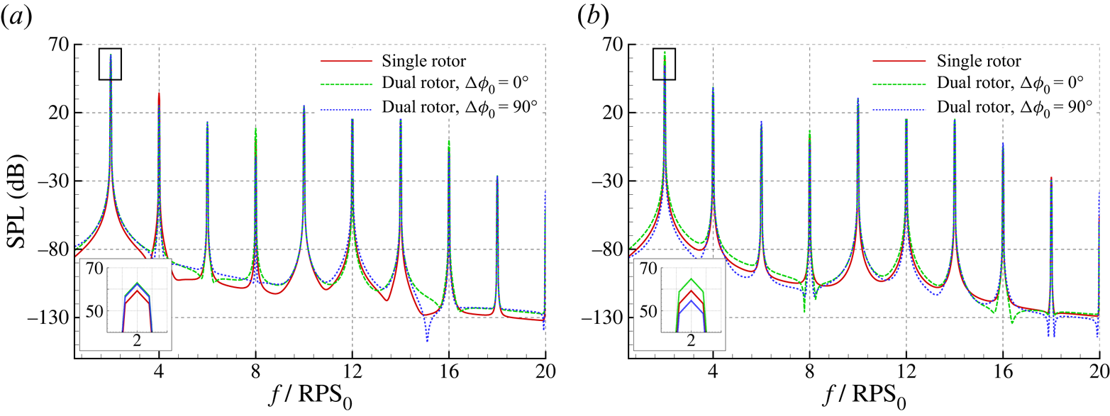
Figure 25. Computed sound spectra of two rotors with periodic fluctuations in RPS with  $f_n=1000$ Hz and $A_n=10^{-3}$. The observers are at (a) $\theta =90^\circ$ and $\varphi =0^\circ$, (b) $\theta =90^\circ$ and $\varphi =90^\circ$.
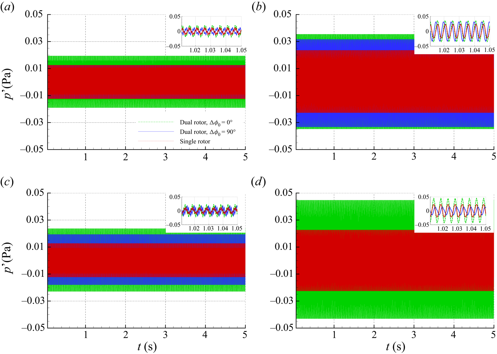
Figure 26. Computed time signals of two rotors with periodic fluctuations in RPS with  $f_n=1000$ Hz and $A_n=10^{-3}$; (a) $\theta =30^\circ$ and $\varphi =0^\circ$, (b) $\theta =90^\circ$ and $\varphi =0^\circ$, (c) $\theta =30^\circ$ and $\varphi =90^\circ$, (d) $\theta =90^\circ$ and $\varphi =90^\circ$.
However, if there is a slight difference in the mean rotation speeds  $\mathrm {RPS}_0^{(1)}$ and $\mathrm {RPS}_0^{(2)}$ due to the static deviations described by $\varepsilon _0$, the phase difference $\Delta \phi$ will vary with time. As a result, the interference effect due to $\Delta \phi _0$ is likely unimportant. To examine this conjecture, we conducted computations with $\mathrm {RPS}_0^{(1)}=99.5$ and $\mathrm {RPS}_0^{(2)}=100.5$ and compare the results for $\Delta \phi _0=0^\circ$ and $90^\circ$, respectively. Moreover, we assume the actual RPS has periodic fluctuations with $f_n=1000$ Hz and $A_n=10^{-3}$. The computed sound spectra at $\varphi =0^\circ$ and $90^\circ$ (and the polar angle is $\theta =90^\circ$ for both cases) are shown in figure 27. Compared with the single rotor, the noise spectra in the dual rotor configuration are higher, but both results for $\Delta \phi _0=0^\circ$ and $\Delta \phi _0=90^\circ$ are close, as expected. In addition, unlike the results shown in figure 25, the difference in the results at different azimuthal angles is small.
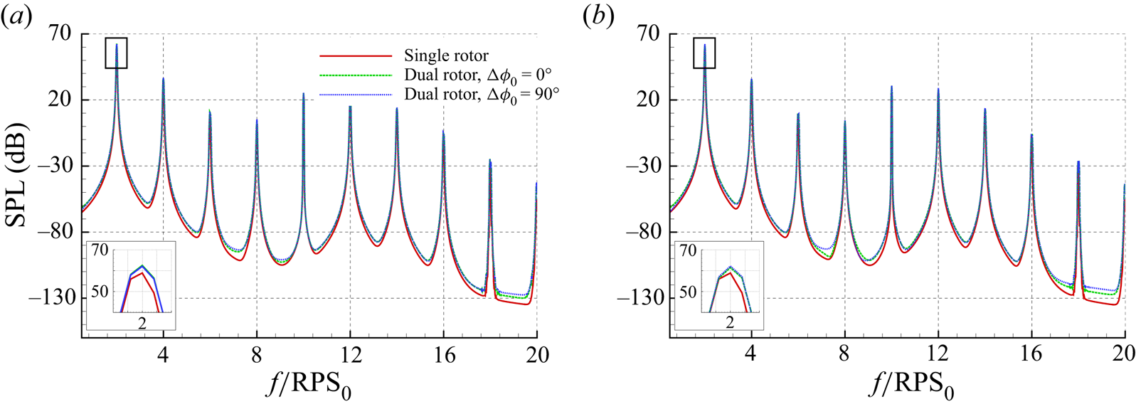
Figure 27. Computed sound spectra of two rotors with slight difference in  $\mathrm {RPS}_0$. The actual RPS is perturbed with periodic fluctuations (with $f_n=1000$ Hz and $A_n=10^{-3}$); (a) $\theta =90^\circ$ and $\varphi =0^\circ$, (b) $\theta =90^\circ$ and ${\varphi =90^\circ}$.
Apart from the periodic fluctuation, we can also study the influence of random fluctuations in the rotation speed. Figure 28 shows the noise spectra with  $f_c=500$ Hz and $A_G=0.5\times 10^{-8}$. Again, the random fluctuations produce bump-type broadband spectra, and some tonal noise is overwhelmed. However, at high frequencies, i.e. $f\ge 10\times \mathrm {RPS}_0$, the peaks are observed again as their levels are higher than the broadband contents. The results with different $\Delta \phi _0$ are close, and the tones at the BPF are nearly unchanged. Meanwhile, the results of both dual rotor configurations are approximately $3$ dB higher than that of the single rotor, similar to the experimental observations (Bu et al. Reference Bu, Wu, Bertin, Fang and Zhong2021). Figure 29 shows comparisons of the time signals of different configurations at different observers in the presence of deviations and unsteady fluctuations in the rotation speed variation. At $\theta =30^\circ$ (downstream), stochastic signals are seen as the random fluctuations of rotation speed that can lead to profound broadband noise contents. For both dual rotor configurations, clusters of sound signals occasionally appear, suggesting that wave packets are formed due to the slight difference in the mean rotation speeds. The phenomenon is more apparent at $\theta =90^\circ$, and the frequency of the wave packet is approximately $1$ Hz, which is the rotation speed difference between the rotors. Consequently, the amplitudes of the sound signals are close despite the phase differences of the wave packets, explaining why the spectra are comparable.
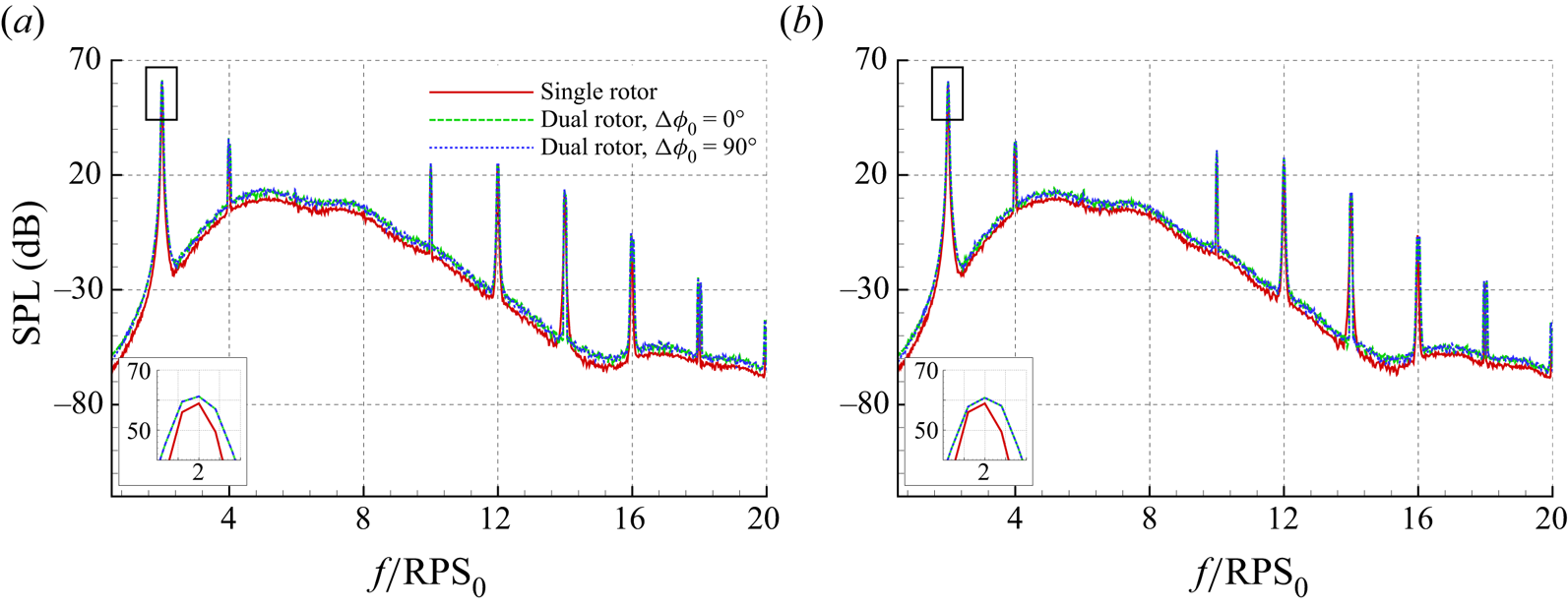
Figure 28. Computed sound spectra of two rotors with slight difference in  $\mathrm {RPS}_0$ of $99.5$ and $100.5$. The actual RPS is perturbed with periodic (with $f_n=1000$ Hz and $A_n=10^{-3}$) and random (with $f_c=500$ Hz and ${A_G=0.5\times 10^{-8}}$) fluctuations; (a) $\theta =90^\circ$ and $\varphi =0^\circ$, (b) $\theta =90^\circ$ and $\varphi =90^\circ$.
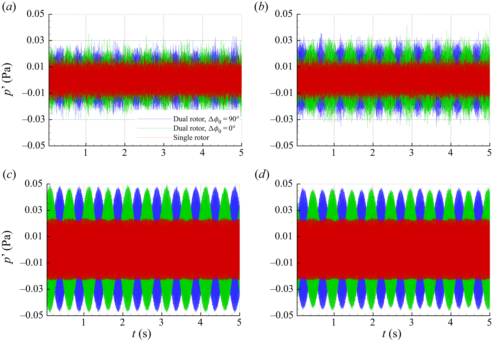
Figure 29. Computed time signals at different observers of two rotors with slight difference in  $\mathrm {RPS}_0$ of $99.5$ and $100.5$. The actual RPS is perturbed with periodic (with $f_n=1000$ Hz and $A_n=10^{-3}$) and random (with $f_c=500$ Hz and $A_G=0.5\times 10^{-8}$) fluctuations; (a) $\theta =30^\circ$ and $\varphi =0^\circ$, (b) $\theta =30^\circ$ and $\varphi =90^\circ$, (c) $\theta =90^\circ$ and $\varphi =0^\circ$, (d) $\theta =90^\circ$ and $\varphi =90^\circ$.
4.2. Counter-rotating dual rotors
We can also study the influence of the counter-rotating dual rotors. In this case, when computing the loadings using (2.18a–c), the value of  ${\zeta }$ is taken as $+1$ and $-1$ for anti-clockwise and clockwise rotating blades, respectively. The rotation direction will affect the source locations and the projections of aerodynamic loading in different directions. Firstly, we assume the averaged rotation speeds of both rotors are $\mathrm {RPS}_0=100$, on top of which there are periodic fluctuations with $A_n=10^{-3}$ and $f_n=500$ Hz. The initial phase difference is $\Delta \phi _0=45^\circ$. Computations are also conducted for the co-rotating dual rotors for comparison. Figure 30 shows the computed spectra at azimuthal observers of $\varphi =0^\circ$ and $90^\circ$, respectively. The polar angle for both observers is $\theta =90^\circ$. At $\varphi =0^\circ$, the results for both co-rotating and counter-rotating configurations are close at $\mathrm {BPF}$. There are discernible differences at higher frequencies, but the levels are much lower. By contrast, significant differences are found at $\varphi =90^\circ$. Particularly, the tonal noise at the BPF is not seen for counter-rotating rotors, which is likely cancelled due to interference. In this work, we also compute the OASPL (from $50$ to $5000$ Hz) at different observer angles to better visualise the directivity. As shown in figure 31, the noise levels have distinguishable patterns for both configurations. Both rotation direction and initial phase angle difference can affect the noise directivity. However, if there are slight differences in the mean rotation speeds, e.g. $\mathrm {RPS}_0=99.5$ and $100.5$, respectively, the interference effect will be significantly altered. As shown in figure 32, the spectra by both co-rotating and counter-rotating configurations are close. Also, for the same polar observer angle $\theta =90^\circ$, the results at different azimuthal angles $\varphi =0^\circ$ and $90^\circ$ are close. Figure 33 shows the directivity patterns of the OASPL computed from $50$ to $5000$ Hz. The noise radiation in different angles is axisymmetric, and the results for co-rotating and counter-rotating rotors are close.
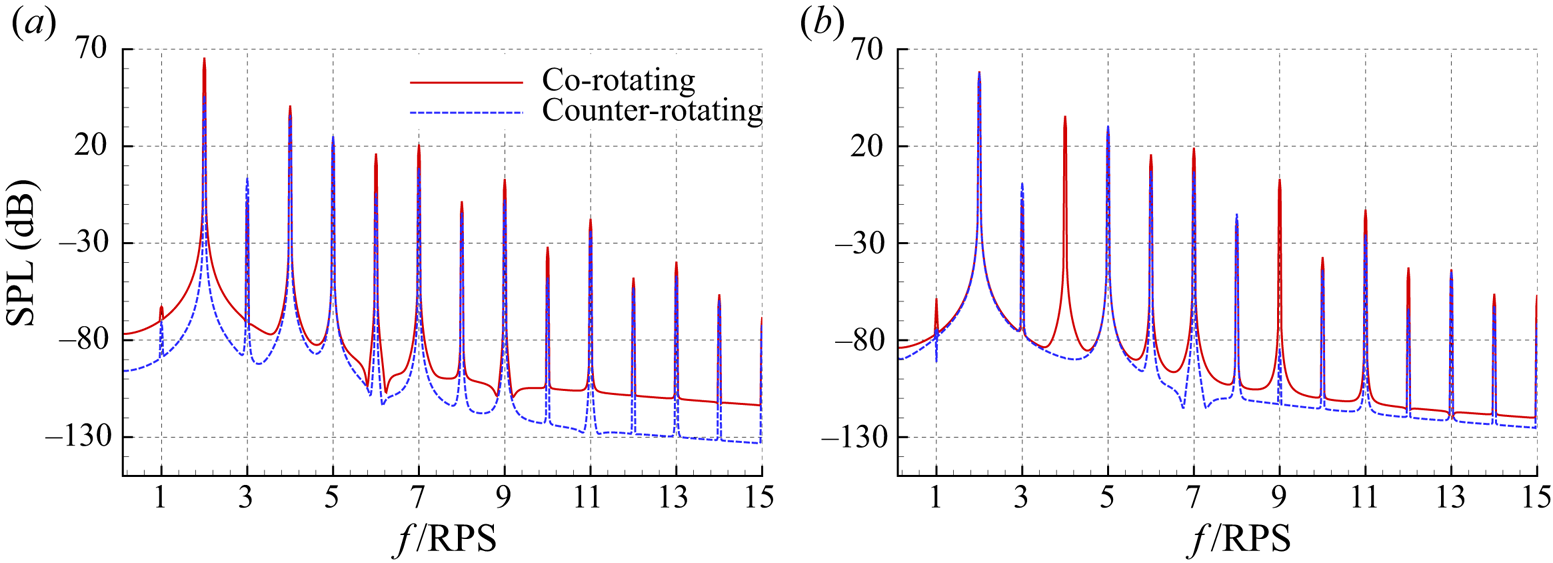
Figure 30. Computed noise spectra for dual rotors with different configurations. Both rotors have the same averaged rotation speed  $\mathrm {RPS}_0=100$. Here, $\Delta \phi _0=45^\circ$ and there are periodic fluctuations in RPS ( $f_n=500$ Hz and $A_n=10^{-3}$); (a) $\theta =90^\circ$ and $\varphi =0^\circ$, (b) $\theta =90^\circ$ and $\varphi =90^\circ$.
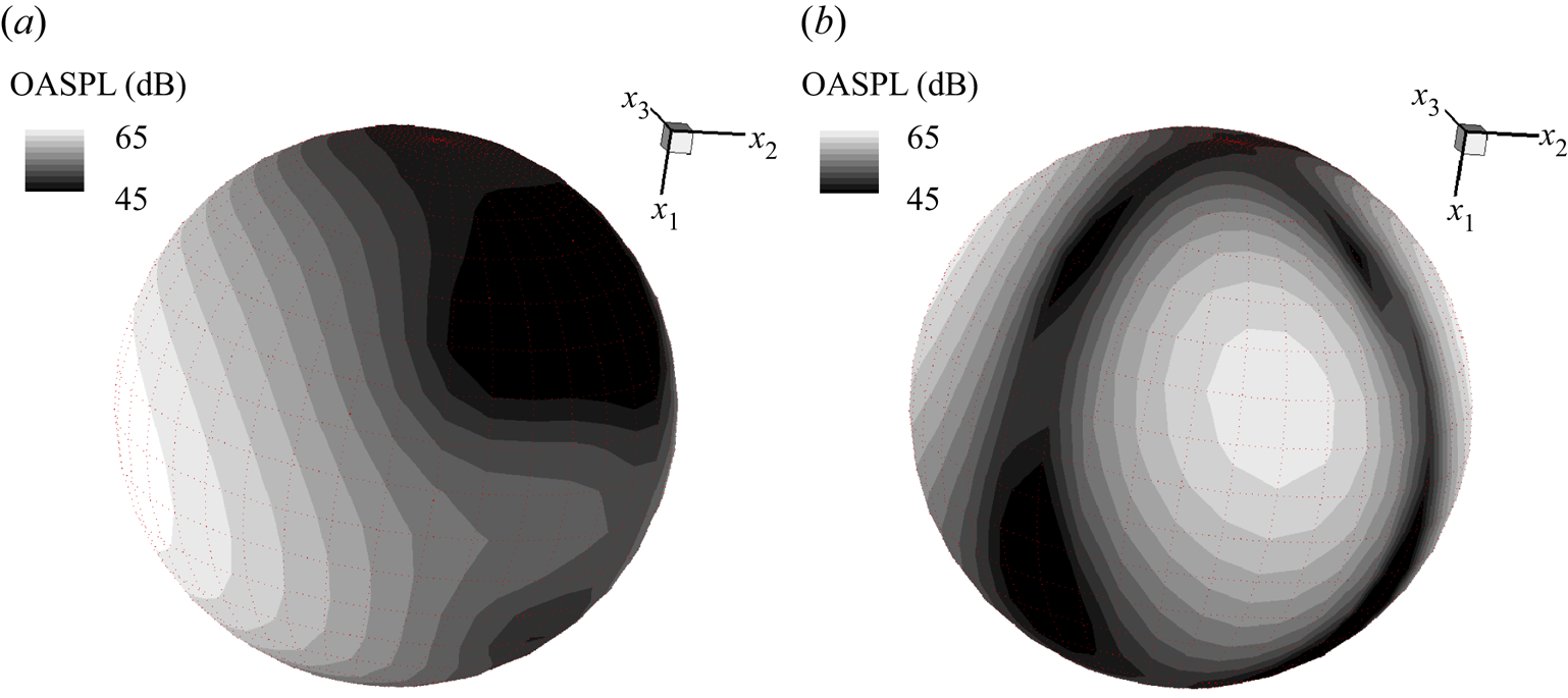
Figure 31. Computed directivity of dual rotors with different configurations. Both rotors have the same averaged rotation speed  $\mathrm {RPS}_0=100$. Here, $\Delta \phi _0=45^\circ$ and there are periodic fluctuations in RPS ( $f_n=500$ Hz and $A_n=10^{-3}$); (a) co-rotating, (b) counter-rotating.

Figure 32. Computed noise spectra for different dual rotor configurations. There mean rotation speeds of the rotors are  $\mathrm {RPS}_0=99.5$ and $100.5$, respectively. Here, $\Delta \phi _0=45^\circ$ and there are periodic fluctuations in RPS ( $f_n=500$ Hz and $A_n=10^{-3}$); (a) $\theta =90^\circ$ and $\varphi =0^\circ$, (b) $\theta =90^\circ$ and $\varphi =90^\circ$.
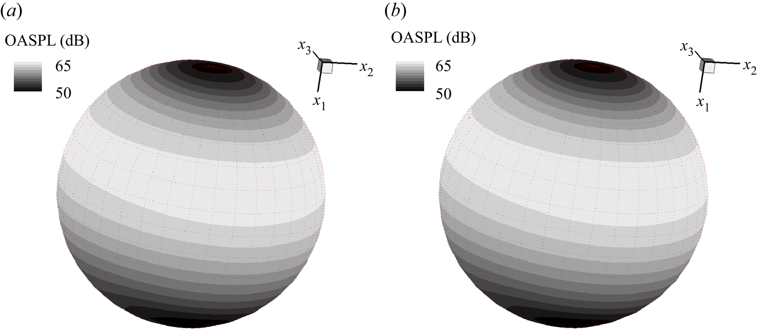
Figure 33. Computed directivity of dual rotors for different dual rotor configurations. The mean rotation speeds of the rotors are  $\mathrm {RPS}_0=99.5$ and $100.5$, respectively. Here, $\Delta \phi _0=45^\circ$ and there are periodic fluctuations in RPS ( $f_n=500$ Hz and $A_n=10^{-3}$); (a) co-rotating, (b) counter-rotating.
5. Summary
This work studies the influence of rotation speed variation and deviation, blade vibration and geometry asymmetry on rotor noise using a time-domain theoretical formulation. The effects of irregular motions are explicitly included in the source coordinate to simplify the computation and efficiently estimate the retarded time. The noise sources are modelled using aerodynamic variables from the BEMT method. The amplitudes of the factors under investigation are assumed to be small. The accuracy of the prediction model is validated by comparing it with experiments and high-fidelity CAA simulations. The rotation speed deviation due to the motor control accuracy can alter the BPF and SPLs. If periodic fluctuations are present, multiple tonal noise components at various frequencies dependent on both BPF and  $f_n$ will be produced. The increment is more significant when $f_n$ is high. If the rotation speed fluctuation is random, broadband-type noise is produced, especially in the upstream and downstream directions. The blade vibration can produce dipole-like noise perpendicular to the rotation plane. The periodic vibration can cause multiple tones, while the random fluctuation can lead to broadband noise increase. The asymmetric geometry of the rotor blades, which can cause a mass imbalance in practice, will lead to tonal noise at multiple frequencies that results from combinations of the RPS and the original peaks in the spectra. The acoustic feature of the dual rotor system is also investigated. If the rotation speeds are identical, the initial phase angle difference $\Delta \phi _0$ and relative rotation directions can significantly affect the sound distribution due to the interference effect. However, if the uncertainty factor is such that slight deviations of the rotation speeds exist for both blades, wave packets are formed due to the rotation speed difference. The phase angle difference varies with time, making the resulting spectra insensitive to $\Delta \phi _0$.
Funding
This work is supported by the Hong Kong Research Grant Council (16202520 and 16206422), National Science Foundation of China (11972029).
Declaration of interests
The authors report no conflict of interest.
Appendix A. Remarks on numerical implementation
At  $\boldsymbol {x}$, the computed sound pressure based on (2.12) is represented at the observer time $t$. The noise contributions by both $Q$ and $L_i$ are evaluated at the retarded time $\tau = t - R/a_\infty$, which, unfortunately, is challenging because $R = R(\boldsymbol {x}(t),\boldsymbol {y}(\tau ))$ is implicitly dependent on the source $\tau$. Moreover, when the rotation speed $\varOmega$ varies with time, the source locations are computed as
 \begin{equation} y_2(\tau) = \eta\cos\left(\phi+\int_0^\tau\varOmega(s)\,\mathrm{d}s\right), \quad y_3(\tau) = \eta\sin\left(\phi+\int_0^\tau\varOmega(s)\,\mathrm{d}s\right), \end{equation}
making the nonlinear integral solution difficult to solve. Alternatively, in practical application, it is common that the observer location  $\boldsymbol {x}$ is unchanged with the observing time $t$. In this case, it is easy to use the source-time-dominant algorithm to account for the retarded time effect (Brentner & Farassat Reference Brentner and Farassat2003). Nevertheless, the detailed procedures for the current formulation is presented for completeness.
For a given source time  $\tau$, the source coordinates $\boldsymbol {y}(\tau )$ can be determined, and the delayed observing time $t$ is explicitly computed as
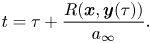 \begin{equation} t = \tau + \frac{R(\boldsymbol{x}, \boldsymbol{y}(\tau))}{a_\infty}. \end{equation}
However, for different source points emitting sound at time  $\tau$, the resulting observing times $t$ at a given observer $\boldsymbol {x}$ are different. For convenience, the blade surface is discretised into $N$ panels, and the centre of each panel is denoted as $\boldsymbol {y}_n \in [\boldsymbol {y}_1, \boldsymbol {y}_2, \ldots, \boldsymbol {y}_N]$. Both the source location and source strength are evaluated at different time steps of $\tau ^m \in [\tau ^1, \tau ^2, \ldots, \tau ^M]$. The two integral kernels in (2.12) are denoted as $\varTheta$ and $\varPi$. The values at the source location $\boldsymbol {y}_n$ and time $\tau ^m$ can be evaluated as $\varTheta _n^m$ and $\varPi _n^m$, respectively. In addition, the corresponding observing time $t_n^m$ is evaluated by using (A2). Therefore, when $m$ ranges from $m=1$ to $M$, we have an array of observing time $\boldsymbol {T}_n = [t_n^1, t_n^2, \ldots, t_n^M]$ and the corresponding arrays of $\varTheta$ and $\varPi$ as
 \begin{equation} \left. \begin{gathered} \boldsymbol{\varTheta}_n(\boldsymbol{T}_n) = [\varTheta_n^1(t_n^1), \varTheta_n^2(t_n^2), \ldots, \varTheta_n^M(t_n^M)],\\ \boldsymbol{\varPi}_n(\boldsymbol{T}_n) = [\varPi_n^1(t_n^1), \varPi_n^2(t_n^2), \ldots, \varPi_n^M(t_n^M)]. \end{gathered} \right\} \end{equation}
Therefore, to ensure noise contribution by all discretised panels can be accounted for, we define a constant observing time array  ${\boldsymbol {T}}=[t^1, t^2, \ldots, t^{\mathscr {M}}]$ with a constant interval of $\Delta t$. Therefore, the values of $\boldsymbol {\varTheta }_n(\boldsymbol {T}_n)$ and $\boldsymbol {\varPi }_n(\boldsymbol {T}_n)$ in (A3) are employed to evaluate the values at the time steps in $\boldsymbol {T}$ (i.e. by using interpolation) as
 \begin{equation} \left. \begin{gathered} \overline{\boldsymbol{\varTheta}_n}(\boldsymbol{T}) = [\overline{\varTheta_n^1}(t^1), \overline{\varTheta_n^2}(t^2), \ldots, \overline{\varTheta_n^\mathscr{M}}(t^\mathscr{M})],\\ \overline{\boldsymbol{\varPi}_n}(\boldsymbol{T}) = [\overline{\varPi_n^1}(t^1), \overline{\varPi_n^2}(t^2), \ldots, \overline{\varPi_n^\mathscr{M}}(t^\mathscr{M})]. \end{gathered} \right\} \end{equation}
Then, an array of sound pressure at  $\boldsymbol {T} = [t^1, t^2, \ldots, t^{\mathscr {M}}]$ can be computed as
 \begin{equation} \boldsymbol{P}(\boldsymbol{x}, \boldsymbol{T}) = [p^\prime(x, t^1),p^\prime(x, t^2), \ldots, p^\prime(x, t^\mathscr{M})] = \frac{\partial}{\partial t}\left(\sum_{n=1}^N \overline{\boldsymbol{\varTheta}_n}(\boldsymbol{T})\right) - \sum_{n=1}^N \overline{\boldsymbol{\varPi}_n}(\boldsymbol{T}), \end{equation}
and the temporal derivative can be easily evaluated by using a finite difference method using the temporal arrays.


 Open access