3.1. Linearised disturbance equations

With the laminar base flow at a given ambient Grashof number $Gr_\infty$, the flow is unstable (or stable) to the perturbation $k$ if the magnitude of its temporal response grows (or decreases) with time. Notably, due to the parallel nature of the unsteady periodic flow, perturbations have no streamwise dependence as would have been seen in the spatially developing flows (Huerre & Monkewitz Reference Huerre and Monkewitz1990). As a result, the perturbations would become unstable (or stable) simultaneously at the same amplification (or damping) rate in the flow anywhere, in which sense the convective instability (or stability) of the flow is global rather than local (see, e.g. later in figures 6 and 8). In this study, the temporal response to the initial perturbation $k$ is tracked by the time trace of the velocity and temperature signals ($\tilde {u}$ and $\tilde {\theta }$) at an arbitrary location $(x_p,y_p)$ within the boundary layer (see also figure 6 of Ke et al. Reference Ke, Williamson, Armfield, McBain and Norris2019). Figure 3 shows the typical temporal responses of the perturbation signals for $k_\infty =0.0486$ ($n=8$) and $k_\infty =0.0971$ ($n=16$) at $Gr_\infty =600$ and $\epsilon = 0.174$. As seen in figure 3, at $Gr_\infty =600$, the oscillatory temporal signals quickly adjust their magnitude to a fully periodic state within $1\sim 2$ temporal periods (i.e. receptivity as the flow receives the external perturbation at $t=0$). In this fully periodic state, the envelope of the temporal signals follow an exponential growth (for $k_\infty =0.0486$) or decay (for $k_\infty =0.0971$) with time. The growth rate of the perturbation signals, termed the amplification rate, is then given by

(3.1)\begin{equation} \sigma_k = \frac{1}{A_t}\frac{\partial A_t}{\partial t}, \end{equation}

where $A_t$ is the instantaneous magnitude of the perturbation signal at time $t$ (i.e. the envelope magnitude in figure 3), which is obtained by taking the fast Fourier transform in the streamwise ($x$) direction at $y=y_p$. For a given combination of $k_\infty$ and $Gr_\infty$, a positive $\sigma _k$ indicates that the temporal response is amplified by the laminar base flow while a negative $\sigma _k$ represents a damped signal. The neutral curve, which characterises the minimal Grashof numbers at which the flow is linearly unstable to a given perturbation $k_\infty$ (i.e. $\sigma _k=0$), can be traced by bisectioning the amplification rates in the $k$–$Gr$ plane.

Figure 3. Temporal responses of the temperature signals at $(x_p,y_p)=(781.6,0.25)$ for base flow at ${Gr_\infty =600}$ and $\epsilon =0.174$ ($\Delta T=50\,{\rm K}$) and (a) $k_\infty =0.0486$ ($n=8$); (b) $k_\infty =0.0971$ ($n=16$). Black dotted lines are the envelopes $\pm A_t$ of the signal that follow the exponential growth or decay; red markers in panel (b) highlight two arbitrarily chosen neighbouring peaks which describes the temporal period $\Delta \tau$ of the signal.

Figure 4 compares the neutral curves ($\sigma _k=0$) for $\epsilon =0.035,0.174$ and $0.347$ with the OB case (Ke et al. Reference Ke, Williamson, Armfield, McBain and Norris2019). While the neutral curves of all the NOB cases show apparent qualitative similarity to the OB case, these curves demonstrate a clear $\epsilon$-dependence: with increasing $\epsilon$, the neutral curve shifts towards higher Grashof numbers at both lower branch ($k_\infty < O(0.1)$) and upper branch ($k_\infty >O(0.1)$). As seen in figure 4, although the critical mode $k_\infty =0.049$ in the lower branch has minimal $\epsilon$-dependency, the critical Grashof number is increased to $Gr_\infty = 473, 536$ and $622$ for $\epsilon = 0.035,0.174$ and $\epsilon =0.347$, respectively, when compared with $Gr_{\infty }=454$ for the OB case. At larger wavenumbers in the upper branch ($k_\infty >O(0.1)$), such a dependency on the temperature difference $\epsilon$ is considerably less than that of the lower branch, where the marginally unstable Grashof number of $k_\infty =0.12$ is increased to $Gr_\infty =948, 959$ and $980$ for $\epsilon = 0.035,0.174$ and $\epsilon =0.347$, respectively. A similar $\epsilon$ dependency of the critical Grashof number has also been reported by Suslov & Paolucci (Reference Suslov and Paolucci1995b) for an NCBL in a differentially heated cavity when using a reference temperature obtained by averaging the hot and cold walls. Based on their eigenvalue analysis, Suslov & Paolucci (Reference Suslov and Paolucci1995b) found that the critical point (i.e. critical $Gr$ and $k$) for the NCBL in a cavity initially locates in the upper branch for relatively low $\epsilon$ and the critical Grashof number would increase with increasing $\epsilon$ – until $\epsilon$ is sufficiently large ($\epsilon >0.54$) such that the critical wavenumber would then shift to the lower branch. However, in the present study, such a drastic change in the critical wavenumber is not observed – we will show later in § 3.2 that this is due to a different instability mechanism in the cavity.

Figure 4. Neutral curve of the NCBL in air with non-Oberbeck–Boussinesq (NOB) effects under various temperature differences, compared with OB results obtained by Ke et al. (Reference Ke, Williamson, Armfield, McBain and Norris2019); dimensionless wavenumber $k_\infty$ and Grashof number $Gr_\infty$ are based on the fluid properties at ambient temperature $T_\infty$.

Since the perturbation wavelength $\lambda$ is fully determined by the mode number $n$ and the streamwise domain length $L_x$, the temporal response signal in figure 3 allows further examination of the wave speed of the perturbation travelling wave $v_p$,

(3.2)\begin{equation} v_p \equiv \frac{\omega}{k}= \frac{\lambda}{\Delta \tau} = \frac{L_x}{n\Delta \tau}, \end{equation}

where $\omega$ is the oscillation frequency and $\Delta \tau$ is the dimensionless time interval between two neighbouring peaks of the response signal, as shown in figure 3(b). Based on linear theory, the interaction between the perturbation and its base flow is linear so that $\Delta \tau$ is constant for a given choice of $Gr_\infty$, $k_\infty$ and $\epsilon$. Figure 5(a,b) compare the maximum base flow velocity $U_m$ with the wave velocity obtained by (3.2) at $Gr_\infty =600$ and $Gr_{\infty }=1000$, respectively. For all temperature differences and base flows considered, the wave velocity decreases with increasing wavenumber and temperature difference $\epsilon$; and the NOB effects on the phase velocity appear more apparent for higher wavenumbers. Notably, Daniels & Patterson (Reference Daniels and Patterson1997, Reference Daniels and Patterson2001) showed that for vertical NCBL flows, the ‘less accurate’ long-wave perturbations will always have a phase speed greater than the maximum base flow velocity ($v_p/U_m\approx 2$); whereas the phase velocity for the short-waves are always less than the maximum base flow velocity ($v_p< U_m$). In this sense, perturbations considered in our study are mostly short-wave disturbances, with a small portion of the ‘less accurate’ intermediate–long waves (since $v_p/U_m\approx 1.2 < 2$ in figure 5a,b) whose accuracy is improved with increasing Grashof (Reynolds) number. At $Gr_\infty =600$, the critical mode $k_\infty =0.049$ (cf. figure 4) is found to have a wave speed close to the maximum base flow velocity $U_m$. This observation is consistent with the findings of Armfield & Patterson (Reference Armfield and Patterson1992) in which the authors showed that the travelling waves amplified by the OB base flow have a wave speed close to the maximum base flow velocity; and with the eigenvalue analysis for the OB case (Ke et al. Reference Ke, Williamson, Armfield, McBain and Norris2019) from which the phase velocity of the critical point is found to be equal to $U_m$. Such a result is seen more clearly in figure 5(c), where the amplification rate $\sigma _k$ is plotted against the wave speed $v_p$. From figure 5(c), only a small band of wavenumbers are amplified by the base flow ($\sigma _k>0$) at $Gr_\infty =600$ – all of which are shown to have a wave speed close to the velocity maximum in the base flow $U_m$, regardless of the temperature differences. Figure 5(c) also shows apparent NOB effects on the amplification rates: the base flow is unstable to $k_\infty =0.049$ ($v_p/U_m=0.98$) and $k_\infty =0.061$ ($v_p/U_m=0.89$) for $\varepsilon \leq 0.174$, but appears stable for $\varepsilon =0.347$ (see inset). At $Gr_{\infty }=1000$, the base flow becomes unstable to a broader band of wavenumbers at the lower phase velocity range at $v_p/U_m\approx 0.55$ (i.e. shorter waves with higher wavenumbers). As shown in figure 5(d), while the critical mode $k_\infty =0.049$ remains the most amplified mode at $Gr_{\infty }=1000$, its phase velocity is decreased to $v_p/U_m=0.88$.

Figure 5. Wave speed of the perturbations $v_p$ against (a,b) wavenumber $k_\infty$ at $Gr_\infty = 600$ and $Gr_{\infty }=1000$; and (c,d) amplification rate $\sigma _k$ at $Gr_{\infty }=600$ and $Gr_{\infty }=1000$. Inset in panel (b) shows the magnified view for the amplified modes; black dotted lines indicates $\sigma _k=0$ and $v_p/U_m=1$.

3.2. Energy budgets for the buoyancy-driven and shear-driven modes

In figure 4, the lower wavenumbers demonstrate a greater sensitivity to the temperature difference $\epsilon$ compared with the upper branch (i.e. larger wavenumbers $k_\infty >O(0.1)$), indicating potential differences in their instability dynamics. In this subsection, we examine the instantaneous perturbation field as well as the perturbation kinetic energy budget of the representative modes in the lower and upper branches to identify and discern the underlying driving mechanisms for these two branches.

Figure 6 depicts the instantaneous contours of the temperature and velocity perturbations of the critical mode $k_\infty =0.049$ at $Gr_\infty =600$, which is representative of the lower branch instabilities. For brevity, only $\epsilon =0.174$ is shown here since all other temperature differences show qualitatively similar structures. From figure 6, it is seen that the velocity fluctuations extend farther out from the wall than the temperature fluctuations, and both instantaneous fluctuation fields have their peaks located beyond the maximum base flow velocity location – indicating that the instability is strongest in the outer part of the boundary layer. There also exists a secondary emerging peak in the velocity perturbation field at $y\approx 16$, which can be seen more clearly in figure 6(c), where the Reynolds normal stress $\overline {\tilde {u}\tilde {u}}$ profile is normalised by its instantaneous maximum (denoted by subscript $_m$). Here, $\bar {\phi }$ denotes the spatial average of flow variable $\phi$ over the homogeneous direction. Although it is difficult to make a direct quantitative comparison due to flow differences, a similar velocity perturbation structure has also been observed in earlier OB stability results for spatially developing natural convection in air (Versteegh & Nieuwstadt Reference Versteegh and Nieuwstadt1998; Aberra et al. Reference Aberra, Armfield, Behnia and McBain2012) and water (Brooker, Patterson & Armfield Reference Brooker, Patterson and Armfield1997; Brooker et al. Reference Brooker, Patterson, Graham and Schöpf2000).

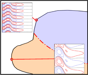
Figure 6. (a) Temperature and (b) velocity perturbation contours of the critical mode $k_\infty =0.049$ at ${Gr_\infty =600}$ and $\varepsilon =0.174$. Contour lines are equally spaced ($10\,\%$, $40\,\%$ and $70\,\%$ of the maximum), and the red solid, blue dashed and black dotted contour lines indicate positive, negative and zero levels. (c) Streamwise Reynolds normal stress $\overline {\tilde {u}\tilde {u}}$ profile normalised by its instantaneous maximum $\overline {\tilde {u}\tilde {u}}_m$. Vertical dash-dotted lines indicate the maximum base flow velocity location $\delta _m$ (green).

To further understand the energy contributions to the perturbation pattern shown in figure 6, we inspect the two-dimensional perturbation energy $E=(\tilde {u}^2+\tilde {v}^2)/2$ budget for this critical mode at $Gr_{\infty }=600$. With streamwise homogeneity, the energy budget equation can be obtained by summing (2.6b) multiplied by $\tilde {u}$ and (2.6c) multiplied by $\tilde {v}$. The resulting budget equation for our temporally developing NCBL reads

(3.3)\begin{equation} \frac{\partial {E}}{\partial t} = \mathcal{P}+\mathcal{B} + \mathcal{D}_b+ \varepsilon_b + \varPi + \varSigma, \end{equation}

where $\mathcal {P}$ is the shear production, $\mathcal {B}$ is the buoyancy production; $\mathcal {D}_b$ is the base flow diffusion; $\varepsilon _b$ is the base flow viscous pseudo dissipation; $\varPi$ is the pressure transport; $\varSigma$ represents the effects due to spatial variation in fluid density and properties. These terms read

(3.4a–c)\begin{gather} \mathcal{P} ={-} \overline{\tilde{u}\tilde{v}}\frac{\partial {U}_b}{\partial y}, \quad \mathcal{B} = \frac{\overline{\tilde{u}\tilde{\rho}}}{\rho_b\epsilon}, \quad \mathcal{D}_b = \frac{1}{2}\frac{\mu_b}{\rho_b}\left(\frac{\partial^2 \overline{\tilde{u}^2} }{\partial y^2}+\frac{4}{3}\frac{\partial^2 \overline{\tilde{v}^2} }{\partial y^2}\right), \end{gather}

(3.4d)\begin{gather} \varepsilon_b ={-}\frac{\mu_b}{\rho_b} \left\{ \overline{ \left(\frac{\partial \tilde{u}_i}{\partial x_j}\right)^2 } +\frac{1}{3} \left[ \delta_{ij}\overline{\left(\frac{\partial \tilde{u}_i}{\partial x_i}\right)^2} +\overline{\frac{\partial \tilde{u}}{\partial x}\frac{\partial \tilde{v}}{\partial y}} +\overline{\frac{\partial \tilde{v}}{\partial x}\frac{\partial \tilde{u}}{\partial y}} \right] \right\}, \end{gather}

(3.4e,f)\begin{gather} \varPi = \frac{1}{\rho_b} \left(\overline{\tilde{p}\frac{\partial \tilde{u}_i}{\partial x_i}}-\frac{\partial \overline{\tilde{v}\tilde{p}}}{\partial y} \right), \quad \varSigma = \mathcal{G}_b +\mathcal{G}_\mu +\mathcal{D}_\mu. \end{gather}

Here, $\mathcal {G}_b$ and $\mathcal {G}_\mu$ are the viscosity gradient effects due to the base flow and local instantaneous viscosity fluctuation, respectively; and $\mathcal {D}_\mu$ is diffusion due to viscosity fluctuation:

(3.5a)\begin{gather} \mathcal{G}_b = \frac{1}{2\rho_b}\frac{\partial \mu_b}{\partial y}\left(\frac{\partial \overline{\tilde{u}^2}}{\partial y}+\frac{4}{3}\frac{\partial \overline{\tilde{v}^2}}{\partial y}+2\overline{\tilde{u}\frac{\partial \tilde{v} }{\partial x}}-\frac{4}{3}\overline{\tilde{v}\frac{\partial \tilde{u}}{\partial x}}\right), \end{gather}

(3.5b,c)\begin{gather} \mathcal{G}_\mu = \frac{1}{\rho_b}\left(\overline{\tilde{u}\frac{\partial \tilde{\mu}}{\partial y}}+\overline{\tilde{v}\frac{\partial \tilde{\mu}}{\partial x}}\right)\frac{\partial U_b}{\partial y},\quad \mathcal{D}_\mu = \frac{1}{\rho_b}\overline{\tilde{\mu}\tilde{u}}\frac{\partial^2 U_b}{\partial y^2}. \end{gather}

Figure 7(a) demonstrates the individual contributors to the energy budget (3.3) for the critical mode $k_\infty =0.049$ at $Gr_\infty =600$. In linear analysis, the perturbations are allowed to grow/decay indefinitely, resulting in a time-dependent scale for the energy budget. However, we note that it is the relative contributions of the terms in (3.4) to the energy budget, rather than the scales, that is of crucial importance to the understanding of the instability mechanisms. In the present study, the energy budgets are normalised in a way such that the base flow viscous diffusion $\mathcal {D}_b$ at the wall ($y=0$) is one. As shown in figure 7(a), the buoyancy production $\mathcal {B}$, being the dominant term in driving the instability, correlates well with the peak of the $\overline {\tilde {u}\tilde {u}}$ seen in figure 6(c); whereas the shear production, $\mathcal {P}$, makes only a small contribution at the peak location and acts as a sink for $y>7$. The production terms shown here behave differently to what is observed in fully turbulent flow where the buoyancy production is usually negligible and negative, and the turbulence is predominantly maintained by shear production (for ${{Pr}}<1$, see Janssen & Armfield Reference Janssen and Armfield1996; Versteegh & Nieuwstadt Reference Versteegh and Nieuwstadt1998; Ke et al. Reference Ke, Williamson, Armfield and Komiya2023). The strong buoyancy production is often seen in the onset of the buoyant instabilities of the unstable atmospheric surface layers (e.g. Leclerc et al. Reference Leclerc, Beissner, Shaw, Den Hartog and Neumann1990, although the gravitational vector aligns differently to the mean flow direction). The high level buoyancy production in figure 7(a) suggests that the instability of the critical mode $k_\infty =0.049$ at $Gr_\infty =600$ is buoyancy driven. However, the effects of local viscosity gradient and fluctuations $\varSigma$ only have minimal effect on the balance. The contributors to $\varSigma$, given by (3.5), are shown in figure 7(b). It is seen that the viscosity fluctuation gradient effect $\mathcal {G}_\mu$ is negligible; while other terms are two orders of magnitude smaller than those in figure 7(a). The buoyancy production is then balanced by base flow viscous diffusion $\mathcal {D}_{b}$ and pressure transport $\varPi$, redistributing the production to the near-wall region and the outer free-shear layer. The sum of the contributors, giving the temporal growth of the perturbation kinetic energy $E$, is shown in figure 7(c). The net energy gain peaks beyond the velocity maximum location $\delta _m$ with a secondary peak at $y\approx 16$. These energy peaks correlate well with those of the instantaneous $\overline {\tilde {u}\tilde {u}}$ profile in figure 6(c).

Figure 7. (a) Perturbation kinetic energy budget for the critical mode in the lower branch $k_\infty =0.049$ at $Gr_\infty =600$ and $\varepsilon =0.174$; (b) contributors involving spatial variation in fluid properties (note change in scale); (c) rate of change $\partial E/\partial t$. All quantities are normalised in such a way that $\mathcal {D}_b=1$ at $y=0$. Vertical dash-dotted lines indicate the maximum base flow velocity location $\delta _m$ (green).

At $Gr_\infty =1000$ and $k_\infty =0.12$, which is representative of the upper branch instabilities, a fundamentally different perturbation field is seen in figure 8. An additional peak in the velocity contour is apparently observed in the near-wall shear layer ($y\approx 2$), as shown in figure 8(b,c). The strong oscillations in the velocity perturbation correlate well with the critical layer locations (marked in violet in figure 8), where the local base flow velocity $U_b\approx 0.55U_m$ (cf. figure 5d) matches the phase velocity $v_p$ of $k_\infty =0.12$ (see also in, e.g. Mack Reference Mack1984; Wall & Wilson Reference Wall and Wilson1996). The existence of such a near-wall peak gives rise to a stronger shear stress and marks the onset of a shear instability for the wall-bounded NCBL (see also figure 8 of Janssen & Armfield Reference Janssen and Armfield1996), rather than the buoyant instability as seen in the lower branch. This can be more clearly seen in the perturbation energy budget, depicted by figure 9(a), where the kinetic energy is shown driven predominantly by shear and buoyancy production near the outer critical layer at $y\approx 8$. Unlike the buoyant instability mode shown in figure 7, for $Gr_{\infty }=1000$ and $k_\infty =0.12$, the shear production grows in strength and demonstrates a similar peak magnitude to that of the buoyancy production $\mathcal {B}$. In the region close to the base flow velocity maximum location $\delta _m$ (green dotted lines in figure 9), $\mathcal {B}$ and $\mathcal {P}$ are slightly negative – the near-wall energy is mainly sustained by the pressure transport from the outer critical layer. Near the production peaks (i.e. outer critical layer), both the base flow viscous dissipation and diffusion are relatively small; and the overall production is balanced by the pressure transport, which redistributes the excessive kinetic energy towards the near-wall and outer shear layers. A similar distribution is also seen by Versteegh & Nieuwstadt (Reference Versteegh and Nieuwstadt1998) for a vertical natural convection in a differentially heated channel, where the near-wall peak of the redistributive pressure term is shown to increase the flow anisotropy near the non-slip wall. The strong pressure transport in the near-wall region (cf. figure 9a) also results in an additional peak for the temporal evolution $\partial E/\partial t$ around the near-wall critical layer, shown in figure 9(c). Figure 9(b) demonstrates the terms involving spatial fluid property variations. Similar to the buoyant instability in figure 7(b), these contributors to $\varSigma$ are at least two orders of magnitude smaller than those of the dominant terms in the kinetic energy budgets. While $\mathcal {G}_\mu$ remains negligible, an extra local maximum is developed for $\mathcal {D}_\mu$ and $\mathcal {G}_b$ close to the critical layer in the near-wall region, which is also suggestive of a change in the energy generation in the near-wall region.

Figure 8. (a) Temperature and (b) velocity perturbation contours of the marginally unstable mode $k_\infty =0.12$ at $Gr_\infty =1000$ and $\varepsilon =0.174$. Contour lines are equally spaced ($10\,\%$, $40\,\%$ and $70\,\%$ of the maximum), and the red solid, blue dashed and black dotted contour lines indicate positive, negative and zero levels. Panel (c) shows the streamwise Reynolds normal stress $\overline {\tilde {u}\tilde {u}}$ profile normalised by its instantaneous maximum $\overline {\tilde {u}\tilde {u}}_m$. Vertical dash-dotted lines indicate the maximum base flow velocity location $\delta _m$ (green) and the locations of the critical layers (violet).

Figure 9. (a) Perturbation kinetic energy budget for the marginally unstable mode $k_\infty =0.12$ at $Gr_\infty =1000$ on the upper branch of the neutral curve ($\varepsilon =0.174$); (b) the contributors involving spatial variation in fluid properties (note change in scale); (c) the rate of change $\partial E/\partial t$. All quantities are normalised in a way such that $\mathcal {D}_b=1$ at $y=0$. Vertical dash-dotted lines indicate the maximum base flow velocity location $\delta _m$ (green); and the locations of the critical layers (violet).

With the kinetic energy budgets, one is able to discern the driving mechanisms for arbitrary modes by comparing the relative contribution (defined by the $\mathcal {R}$) of shear production $\mathcal {P}$ to the buoyancy production $\mathcal {B}$ across the boundary layer,

(3.6)\begin{equation} \mathcal{R} = \frac{\int_{0}^{\infty} \mathcal{P} \,\mathrm{d} y }{\int_{0}^{\infty}\mathcal{B} \,\mathrm{d} y}. \end{equation}

The production ratio $\mathcal {R}$ conveniently distinguishes the flow regimes by the relative strength that drives the instabilities on the neutral curve: $\mathcal {R}>1$ for shear-driven instability and $\mathcal {R}<1$ for buoyancy-driven instability. As shown in figure 10(a), the shear-driven instability occurs at relatively large wavenumbers in the upper branch and it occupies increasingly greater area in the $k$–$Gr$ plane with increasing $Gr_\infty$ as the base flow gains more momentum. The buoyant instability, however, mainly happens at relatively low $Gr_{\infty }$ and small wavenumbers $k_\infty$ in the lower branch. This result is consistent with the findings in a differentially heated cavity (Suslov & Paolucci Reference Suslov and Paolucci1995b). However, we shall point out that the onset of shear and buoyant modes observed by Suslov & Paolucci (Reference Suslov and Paolucci1995b) may be due to a different mechanism – Suslov & Paolucci (Reference Suslov and Paolucci1995b) observed that the flow is first unstable to the shear-driven modes in the upper branch due to the breakdown of odd symmetry at the mid-span of the differentially heated cavity. For NCBLs in differentially heated cavities and channels, the shear-driven instability is typically stationary (with a phase velocity of $v_p=0$), while the buoyancy-driven modes are oscillatory in the Boussinesq limit (Suslov & Paolucci Reference Suslov and Paolucci1995b; McBain & Armfield Reference McBain and Armfield2003). With NOB effects, Suslov & Paolucci (Reference Suslov and Paolucci1995b) showed that the resulting shear-driven mode has a negative wave speed $v_p<0$ (i.e. propagating against the base flow) for cavity flows; whereas in the present study, perturbation waves are travelling in the direction of the base flow ($v_p>0$, cf. figure 5). Notably, for our NCBL, there also exists a region at low wavenumbers where the shear production is negative (resulting in $\mathcal {R}<0$). In this region, the instability is driven entirely by buoyancy (see, e.g. the critical mode budget in figure 7a, where $\mathcal {P}$ has a peak value an order of magnitude smaller than that of $\mathcal {B}$ and acts as a sink in the outer shear layer). Figure 10(b) depicts the temperature difference effects on the $\mathcal {R}$ contours. Evidently, with increasing temperature difference $\epsilon$, the $\mathcal {R}$ contours are shifted to higher $Gr_{\infty }$ and larger $k_\infty$, effectively expanding the buoyancy-driven region in the $k$–$Gr$ plane. Such a result is not surprising as the buoyancy effect becomes increasingly strong with greater temperature differences and therefore results in a broadened buoyancy-driven instability region in figure 10. The growing strength of buoyant instability with increasing $\epsilon$ is also seen by Suslov & Paolucci (Reference Suslov and Paolucci1995b), where the critical point (minimum $Gr_{\infty }$ at which the flow becomes marginally unstable to any perturbation) changes from shear driven to buoyancy driven when $\epsilon$ is large enough. However, for the temperature differences considered here up to $\epsilon =0.347$, we have not observed such a sudden change of the critical mode since the unsteady NCBL is unstable to the buoyancy-driven mode first and larger $\epsilon$ would only strengthen the buoyant instability – we conjecture that such a change in critical mode is more likely to occur in NCBLs with higher Prandtl number where the flow might become unstable to the upper shear-driven branch first.

Figure 10. (a) Ratio of integrated shear production to the buoyancy production overlaid on the neutral curve for $\epsilon =0.174$. Red dash-dotted line ($\mathcal {R}=1$) divides the shear-driven (upper) and buoyancy-driven (lower) instability regions; blue dotted line indicates $\mathcal {R}=0$, below which shear production is negative $\mathcal {P}<0$. (b) Dependence of $\mathcal {R}=1$ and $\mathcal {R}=0$ contours on the temperature differences. Colours represent the temperature differences: (green) $\epsilon =0.035$, (blue) $\epsilon =0.174$ and (red) $\epsilon =0.347$; dash-dotted lines represent $\mathcal {R}=1$ and dotted lines denote $\mathcal {R}=0$.

3.3. Neutral curves re-normalised using the film temperature

In the context of NCBL literature, flow field characterisation parameters, such as Grashof number $Gr$ and Rayleigh number $Ra$, are often evaluated at the film temperature ${T_f=(T_w+T_\infty )/2}$ for practical purposes. Earlier investigations on the NOB NCBL revealed that greater temperature differences would destabilise the gaseous boundary layer flows with a lower transition Grashof number when evaluated at $T_f$ (e.g. Chenoweth & Paolucci Reference Chenoweth and Paolucci1986; Sabhapathy & Cheng Reference Sabhapathy and Cheng1986; Jiin-Yuh & Mollendorf Reference Jiin-Yuh and Mollendorf1988), suggesting an earlier onset of instabilities at larger $\epsilon$ for air. As shown in figure 4(a), our linear stability results show that a higher $Gr_\infty$ is needed to trigger the instability for greater temperature differences $\epsilon$, i.e. increasing $\epsilon$ would stabilise the NCBL. However, these results do not imply that our calculations contradict earlier investigations as the neutral curves in figure 4 are normalised using the ambient temperature. Figure 4(a) can be re-normalised using fluid properties at $T_f$, as shown in figure 11. Here, $k_f$ and $Gr_f$ are the dimensionless wavenumber and the film Grashof number,

(3.7a,b)\begin{equation} k_f = k_\infty\left(\frac{L_{s,\infty}}{L_{s,f}}\right)=k_\infty \left(\frac{\kappa_\infty\rho_f}{\kappa_f\rho_\infty}\right)^{2/3},\quad Gr_f=Gr_\infty\left(\frac{\mu_\infty\rho_f}{\mu_f\rho_\infty}\right)^2. \end{equation}

As depicted by figure 11, while the neutral curves for the $\varepsilon$-range reported still share a similar shape, it is evident that with increasing $\epsilon$, the critical Grashof number decreases – indicating the air NCBL flow, when evaluated by the film temperature $T_f$, is destabilised when a larger temperature difference is applied to the base flow. Unlike figure 4(a), when normalised by $T_f$, the shear-driven instability demonstrates a greater dependence on the temperature difference $\epsilon$. For instance, the marginally unstable Grashof number for $k_f\approx 0.12$ is decreased from $Gr_f=892$ at $\epsilon =0.035$ to $Gr_{f}=564$ at $\epsilon =0.347$; however, the critical Grashof number for the buoyancy-driven instability in the lower branch decreases slightly to $Gr_{f}=355$ at $\epsilon =0.347$ from $Gr_{f}=445$ at $\epsilon =0.035$. Figure 11 indicates when evaluating at $T_f$, the NOB effects due to heating are to destabilise the air flow, prominent for the shear-driven modes but to a lesser extent for the buoyancy-driven modes. These results are consistent with the earlier linear stability investigations for NCBLs along vertical plates, e.g. Sabhapathy & Cheng (Reference Sabhapathy and Cheng1986) and Jiin-Yuh & Mollendorf (Reference Jiin-Yuh and Mollendorf1988) reported heating (decreasing viscosity and conductivity) would stabilise the liquid flows ($7\leq {{Pr}}\leq 100$). Note the viscosity and conductivity for liquid flows decrease with increasing temperature, which is different from the gaseous flow described by Sutherland's law.

Figure 11. Neutral curves and $\mathcal {R}=1$, $\mathcal {R}=0$ contours re-normalised using film temperature $T_f= (T_w+T_\infty )/2$. Colours represent the temperature differences: (green) $\epsilon =0.035$, (blue) $\epsilon =0.174$ and (red) $\epsilon =0.347$; dash-dotted lines represent $\mathcal {R}=1$; dotted lines denote $\mathcal {R}=0$.

3.4. Direct stability analysis

With the linear stability results obtained in § 3.1, the extent of the linear regime where a perturbation of choice, $k_\infty$, interacts linearly with the base flow can be identified by comparing the direct numerical solution to the perturbed system (2.1) in three-dimensional form. By imposing the boundary conditions as impermeable isothermal wall at $y=0$, and the quiescent ambient at $y=L_y$,

(3.8a)\begin{gather} u=v=w=0,\quad \theta = \theta_w, \quad \text{at}\ y=0, \end{gather}

(3.8b)\begin{gather} \frac{\partial{u}}{\partial y} =v= \frac{\partial{w}}{\partial y} =\theta = 0, \quad \text{at}\ y=L_y. \end{gather}

With periodic boundary condition applied in the spanwise $z$ direction, the three-dimensional direct numerical simulation (DNS) is carried out in an $L_x\times L_y \times L_z = 1035L_{s,\infty }\times 207 L_{s,\infty } \times 129 L_{s,\infty }$ computational domain with an $N_x \times N_y \times N_z = 1024\times 256 \times 128$ Cartesian grid (stretched in the $y$ direction but uniform in the homogeneous directions $x$ and $z$, with the same stretching strategy as used in the linear stability runs in § 2). The temperature perturbation, given by (2.7), is fed into the flow at $Gr_\infty =250$ with $n=8$ (so that $k_\infty =0.049$ is obtained) and $A_n=10^{-3}$. The ambient temperature is set to $T_\infty =288\,{\rm K}$ and the bulk temperature difference is set to $\Delta T=100\,{\rm K}$ to enable a direct comparison with the linear stability results for $\varepsilon =0.347$. For the DNS, the perturbation field of a flow variable $\tilde {\phi }$ is obtained by subtracting the homogeneous spatial average of a flow variable $\bar {\phi }$ from its instantaneous value $\phi$, i.e. $\tilde {\phi } = \phi -\bar {\phi }$. Figure 12(a) shows the instantaneous and the fluctuation signal of the temperature at $(x_p,y_p,z_p)=(781.6,0.25,64.5)$. Although the temperature fluctuation demonstrates a similar oscillatory behaviour as shown in the linearised solutions (e.g. figure 3), nonlinear developments become visible at $t\approx 120$ (which corresponds to $Gr_\infty \approx 2.2\times 10^4$). This can be clearly seen in figure 12(b), where the instantaneous amplitude of the temperature fluctuation signal $A_t$ is plotted against the Grashof number $Gr_\infty$. From figure 12(b), the temporal signal follows an adjustment immediately after the temperature perturbation is fed into the flow. Similar adjustments are also seen in the linearised solutions (cf. figure 3) and typically end at $t\approx 50$. During this process, the temperature fluctuation is tuned to an appropriate magnitude and phase condition in a way that it does not follow the linear amplification or decay as the boundary layer receives external artificial perturbation (also known as the receptivity process, see Reed, Saric & Arnal Reference Reed, Saric and Arnal1996; Saric, Reed & Kerschen Reference Saric, Reed and Kerschen2002; Ke et al. Reference Ke, Williamson, Armfield, McBain and Norris2019). For the unsteady DNS, a development time of $t=50$ for the base flow corresponds to $Gr_{\infty }\approx 7\times 10^3$, as shown in figure 12(b). Beyond this inevitable initial receptivity, the temperature fluctuation is amplified almost linearly in the log–log plot as the mean flow continues to develop – up until the onset of nonlinearity at $Gr_\infty \approx 1.7\times 10^4$.

Figure 12. (a) Temporal signal of the instantaneous temperature $\theta$ (left axis) and the temperature fluctuation $\tilde {\theta }$ (right axis) which is obtained by subtracting the spatial average $\bar {\theta }$ from the instantaneous value $\theta$; (b) instantaneous magnitude of the temperature fluctuation against the ambient Grashof number $Gr_{\infty }$.

This limit of the linear range can be seen in figure 13, where the amplification rate, $\sigma _k$, of the LNS is compared with the DNS results. With increasing $\epsilon$, the NOB LNS solutions are shown to have a slightly lower amplification rate than that of the OB case for $Gr_{\infty }<5\times 10^3$; however, at greater $Gr_{\infty }$, the perturbation is amplified at a much faster rate. This indicates that a larger bulk characteristic temperature difference would result in the infinitesimal perturbations being amplified more quickly as the flow continues to evolve in time, and potentially would lead to an earlier onset of nonlinearities and laminar–turbulent transition. The DNS data, however, show good agreement with the linear stability results after its initial receptivity process at $Gr_{\infty }\approx 7\times 10^3$. Notably, there are instantaneous fluctuations showing up in the DNS amplification data as there have been weakly nonlinear effects due to the interactions between the perturbation field and property/density fluctuations, all of which, being the higher order nonlinear terms, have been dropped in the linear disturbance modelling (2.6). However, this nonlinear effect is considered negligibly weak since it only has minimal impact on the amplification rates obtained by DNS. By comparing the amplification rates obtained from the DNS and the linear stability results, the linear regime for $\varepsilon =0.347$ is identified to be up until $Gr_\infty \approx 1.7\times 10^4$ (or, equivalently $Gr_{f}\approx 9.7\times 10^3$ when evaluated using $T_f$) – beyond this point, the linear stability result diverges from the DNS data since nonlinearity takes over the perturbation amplification mechanism. The onset of nonlinearity, when evaluated at film temperature, is found to be earlier than that of the OB case, whose linear range extends up to $Gr=1.3\times 10^4$ for an initial perturbation amplitude of $A_n=10^{-3}$ (Ke et al. Reference Ke, Williamson, Armfield, McBain and Norris2019). Such a result is indeed consistent with the observation of Siebers et al. (Reference Siebers, Moffatt and Schwind1985), where they experimentally found that for a fixed $T_\infty$, the film Grashof number $Gr_f$ at which transition occurs decreases with increasing wall temperature $T_w$ (and thus the temperature difference $\Delta T$).

Figure 13. Amplification rate $\sigma _k$ comparison for wavenumber $k_\infty \approx 0.049$. Lines represent the OB case based on the Orr–Sommerfeld eigenvalue analysis of Ke et al. (Reference Ke, Williamson, Armfield, McBain and Norris2019) (black dotted), and linear stability (LNS) results obtained in § 3.1 for $\epsilon =0.035$, $\epsilon =0.174$ and $\epsilon =0.347$. Markers denote the direct stability results for $\varepsilon =0.347$. Vertical lines mark the end of receptivity tuning (left) and the start of nonlinear regime (right).