


1. Introduction
Stars with a mass above ∼0.5 M⊙ but below M up,C can form a compact carbon–oxygen (CO) core supported by the degenerate electron pressure, where M up,C ∼6–9 M⊙ depending on the metallicity [e.g., Umeda et al. (Reference Umeda, Nomoto, Tsuru and Matsumoto2002)]. Hereafter, we use the solar metallicity value of M up,C ∼8 M⊙ [e.g., Umeda et al. (Reference Umeda, Nomoto, Tsuru and Matsumoto2002)] for simplicity. It is observed as an Asymptotic Giant Branch (AGB) star owing to its extended envelope.
An electron-degenerate oxygen–neon–magnesium (ONeMg) core forms in single stars of masses from M up,C to M up,ONecore. Here, M up,ONecore depends on metallicity and thermal pulses of He shell burning, which have not been fully explored yet. Hereafter, we use the solar metallicity value of M up,ONecore ∼ 10 M⊙ [e.g., Nomoto, Thielemann, & Yokoi (Reference Nomoto, Thielemann and Yokoi1984) and Jones et al. (Reference Jones2013)] for simplicity [See, e.g., Nomoto, Kobayashi & Tominaga (Reference Nomoto, Kobayashi and Tominaga2013) for the evolution of more massive stars].
An ONeMg core can also form in a binary star. The mass of the progenitor that forms the degenerate ONeMg core depends on the parameters of binary system (see Section 2).
In this review, we shall summarise the recent progress of ECSN modelling as follows [see also Nomoto & Leung (Reference Nomoto and Leung2017)]. In Section 2, the presupernova evolution of 8–10 M⊙ stars is reviewed. In Section 3, the governing physics of ECSN is reviewed. In Section 4, we review how different physics components contribute to the ECSN. In particular, this includes the summary of the treatment of flame, turbulent deflagration and electron capture and how they participate to the explode/collapse bifurcation of ECSN. In Section 5 and 6, we review how these physics components and the initial models determine the final fate of the AGB stars. In Section 7, the observables of low-energy explosions as the outcome of collapse such as SN light curves to compare with the Crab supernova 1054 and the neutron star properties are summarised.
2. Evolution of Super AGB Stars
2.1. Formation of degenerate ONeMg cores
2.1.1. Single-star scenario
In Figures 1–3, the chemical evolutions of stars in the mass range of M up,C < M < M up,ONcore and their mass dependence are shown for the case of single star. These stars have 8.8, 9.6, and 10.4 M⊙ on the main-sequence and form He cores of 2.2, 2.4, and 2.6 M⊙, respectively.
Figure 1. The chemical evolution diagram of a 8.8 M⊙ star starting from He burning until the formation of a degenerate O–Ne–Mg core [see also Nomoto et al. (Reference Nomoto1982) and Nomoto (Reference Nomoto1987)]. Notice that the shaded region corresponds to the surface convection zone, which can reach the He layer and remove the He layer known as the second dredge-up. The curly shape shading corresponds to different burning stages.
Figure 2. Similar to Figure 1 but for the 9.6 M⊙ star (Nomoto Reference Nomoto1984).

Figure 3. Similar to Figure 1 but for the 10.4 M⊙ star. The evolution up to ONe shell burning is included (Nomoto Reference Nomoto1984).
In the CO cores of these stars, electrons are partially degenerate and the stars are partially supported by the thermal pressure. In such semi-degenerate CO cores, neutrino cooling forms a temperature inversion in the central region. For the CO coremass greater than 1.06 M⊙, the C-rich matter outside the core begins to burn [See Kawai, Saio & Nomoto (Reference Kawai, Saio and Nomoto1988) for the CO white dwarf case]. Owing to heat conduction, the C-burning propagates towards to the core (Figures 1 and 2) (Nomoto Reference Nomoto1984; Timmes & Woosley Reference Timmes and Woosley1992); See Saio & Nomoto (Reference Saio and Nomoto1985, Reference Saio and Nomoto1998) for the CO white dwarf case.
After C is exhausted in the central region, a semi-degenerate ONeMg core forms. We show in Figure 4 (Nomoto Reference Nomoto1984) the central temperature against central density for the Ne core to present the critical mass of Ne-burning. The evolution of cores with masses 1.30, 1.365, and 1.37 M⊙ is shown here with the solid lines being the quantity at centre and dashed lines being that of the zone with the global maximum value. For the core models with a mass below 1.37 M⊙, the central and maximum temperature rise and then drop as density increases. The later temperature drops because of the rapid neutrino cooling. The higher maximum temperature than the central temperature shows that during the contraction, the temperature inversion appears. The temperature, however, is still not high enough to trigger Ne-ignition. The energy generated by this burning channel is slower than the local energy loss, especially by thermal neutrino loss. On the other hand, at 1.37 M⊙, the global maximum temperature can reach above 109.1 K (the dotted line), showing that the Ne begins to ignite off-centre.
Figure 4. The central temperature against central density for the pure neon stars model of 1.30, 1.365, and 1.37 M⊙ (Nomoto Reference Nomoto1984). The temperature and density in the centre are represented by solid lines; the maximum value across the star is shown by dashed-line. The Ne-ignition line, where the energy release rate by Ne-burn exceeds the local energy loss, is marked by the dotted line. The model of 1.37 M⊙ characterises the onset of Ne burning.
The CO core mass does not exceed 1.37 M⊙ in the 8.8 and 9.6 M⊙ stars, so that Ne-burning cannot be triggered in these stellar models (Figures 1 and 2). The lack of Ne-burning makes the ONeMg core strongly degenerate. For the 8.8 M⊙ star, the He-layer is dredged up to form a very thin He layer. The AGB stars are one of the possible sources of s-process elements, such as Bi, Y, and Pb. For the 9.6 M⊙ star, He shell-burning is ignited to produce C before the He layer is dredged up (Figure 2). Eventually, these stars become super-AGB (SAGB) stars (e.g., Siess Reference Siess2007).
For the 10.4 M⊙ star, off-centre Ne burning is ignited and the Ne flame propagates inward as the core contracts to increase the core temperature (Figure 3). (Note the difference from C-flame which propagates inward owing to heat conduction.) Ne-shell burning gets stronger and stronger, and its outcome would be interesting (Nomoto & Hashimoto Reference Nomoto and Hashimoto1988).
The evolution of Ne-burning is unlike its more massive counterpart because electrons in the ONeMg core are semi-degenerate. A temperature inversion appears in the central region because neutrino cooling is faster for higher densities. Such an inversion prohibits Ne to be ignited at centre. After the off centre ignition, Ne burning gradually propagates inwards by compression during gravitational contraction. This forms a Si-rich shell. For helium core of about 2.8 M⊙, the core has a density ∼108 g cm−3, which is strongly degenerate. Ne-burning can become explosive to cause a large-scale expansion of the star. This might lead to the ejection of outer H- or He-envelope, which might be observationally significant. It is therefore an interesting topic to follow the propagation of Ne-burning.
As a result of H and He shell burning, a C-rich matter accumulates on the surface of the ONeMg core. The C+ONeMg core mass increases and the central density follows. The luminosity rises following the core mass—luminosity relation.
We remind that the exact fate of the SAGB star depends on how fast the mass loss reduces the envelope mass, before the core mass increases the ONeMg core until Ne-ignition. In general, the mass loss of the sAGB star is dominated by three mechanisms. First, it is the dust-induced mass loss. During dredge-up, the carbon in the inner layer is transported to the surface. This strongly enhances the opacity. Second, the pulsation of the star is dynamically unstable. The pulsation can also lead to mass ejection of the surface layer. Third, the magnetic field near the surface can trigger mass loss due to its energy deposition.
2.1.2. Binary star scenario
In a binary star system, the degenerate ONeMg core evolves in a helium star and could give rise to the stripped-envelope ECSN. Podsiadlowski et al. (Reference Podsiadlowski, Langer, Poelarends, Rappaport, Heger and Pfahl2004) estimated that the main-sequence mass range of such a channel to reach ECSNe is as broad as 8–17 M⊙, Here, compared to the single-star scenario, a higher mass main-sequence star may form a smaller mass helium core in the ECSN mass range, because the mass transfer removes the hydrogen envelope before the mass ratio between the helium core and the main-sequence grows to the single-star case. The exact mass range depends on when the Roche-lobe overflow occurs, i.e., near the end of core hydrogen burning, or during hydrogen shell burning, thus depending on the binary parameter (Kippenhahn & Weigert Reference Kippenhahn and Weigert1967).
Tauris, Langer, & Podsiadlowski (Reference Tauris, Langer and Podsiadlowski2015) estimated the He core mass range for allowing ECSN as 2.6–2.9 M⊙, depending on the rotation period, being a little wider than the single-star case. Moriya & Eldridge (Reference Moriya and Eldridge2016) estimated that stripped-envelope ECSNe can make up about 1% of the total supernova population.
We note that the helium star that forms degenerate ONeMg core expands to lose its helium envelope to the companion in some binary systems, which needs to be carefully examined for a more accurate estimate of the ECSN rate.
In the recent large-scale survey of binary star evolution models (Poelarends et al. Reference Poelarends, Wurtz, Tarka, Cole Adams and Hills2017), by considering the initial rotation period (inter-star distance) and the progenitor mass, depending on the efficiency of mass transfer by Roche-lobe flow, a total of five possibilities are observed, namely (1) Short-P contact, (2) Long-P contact, (3) ONe WD, (4) CCSN, and (5) ECSN. In particular, the ECSN channel is likely to occur in the mass range of ∼13.5–15.2 M⊙ for the primary star, with a rotating period of 4 d and above, or ∼15.2–17.6 M⊙ for the primary star with a shorter rotation period (∼2.5–3.5 d). Notice that the exact value depends on both the efficiency of mass transfer and the mass ratio. In general, the mass range for forming ONeMg core and hence ECSN has a higher value 13.5–17.6 M⊙. More recently, Siess and Lebreully (Reference Siess and Lebreuilly2018) studied Case A and B binary evolution and concluded that these cases produce new but narrow channels to ECSNe.
2.2. Formation and evolution of ONeMg white dwarfs
In the scenario where mass loss overwhelms the mass gain by H- and He-shell burning, the core will not be massive enough for further advanced burning. A single ONeMg white dwarf (WD) forms. This scenario applies to the mass range of M up,C < M ⪅ M up,Ne where M up,Ne = 9 ± 1 M⊙ is the upper mass limit of the progenitor of an ONeMg WD. The exact value of this quantity is metallicity dependent and is found to be smaller for lower metallicities (Siess Reference Siess2007; Pumo et al. Reference Pumo2009; Langer Reference Langer2012; Doherty et al. Reference Doherty, Gil-Pons, Siess, Lattanzio and Lau2015).
Besides the single-star scenario, in the binary scenario, the SAGB also plays an important role to its companion star via binary interaction. The typical ONeMg core has a resultant mass between 1.1 and 1.37 M⊙. For the ONeMg core exceeds ∼1.367 M⊙, the ECSN is capable to start spontaneously (Takahashi, Yoshida, & Umeda Reference Takahashi, Yoshida and Umeda2013). In such interaction, the ONeMg core is not disrupted because of the very strong gravitational potential compared to its former sparsely distributed SAGB star. As a result, in such a close binary system, the ONeMg core can always accrete mass from its companion through Roche-lobe overflow.
On one hand, if the mass transfer is slow, the surface matter has sufficient time to heat up. This creates a nova event. Such nova is known to be Ne-nova because during accretion, the dredge-up by the convective layer can penetrate deep down to the Ne layer. On the other hand, when the mass transfer rate is fast, the ONeMg WD does not have time to remove the accreted mass by nova, the density increases faster than the temperature in the centre. The electron capture in the core will directly trigger the accretion-induced collapse (AIC), which is another way of forming a low mass NS.
2.3. Formation and evolution of ONeMg cores
Electron capture supernovae (ECSNe) can form for stars with a mass M up,C < M ⪅ M up,Ne, where M up,One ≈ 10 M⊙ stands for the upper mass limit where ONe remains not burnt in the core. Due to the faster H and He shell burning compared to the mass loss, the ONeMg core mass can reach 1.38 M⊙. This also leads to a higher central density. Notice that in such high density matter, the electron becomes extremely degenerate. The high Fermi energy can exceed the threshold for electron capture on the C-burning product, such as the nuclei of 25Mg, 23Na, 24Mg, 20Ne, and 16O. Usually, the electron capture is a one-way process because the isotope will not convert back to its mother nuclei. However, for ECSNe, the particular density and hence Fermi energy allow the transition from the mother nucleus in the ground state to the daughter nucleus also in the ground state. These nuclei pairs include the odd mass numbers nuclei A = 23 and 25, i.e., 25Mg–25Na, 23Na–23Ne, and 25Na–25Ne. Such pairing allows repetitive electron capture-beta decay on the URCA shell (electron captures and β decays). As a more detailed example, in the deeper layer 25Mg nuclei capture surrounding electrons and form 25Na. The 25Na nuclei are in the excited state and later emit gamma-ray when decay into its ground state. This process heats up the surrounding matter and creates an upward flow, which also brings 25Na away from the layer. As 25Na nuclei move away from the core, they experience a drop in the surrounding density. The electron Fermi energy drops accordingly. The electron capture becomes slower than the β-decay. Then the 25Na decays into 25Mg by β-decay. They follow the convective flow and return to the original layer. In the whole process, two neutrinos are emitted. The neutrinos can freely escape from the star and therefore the star has a net energy loss. The energy loss by radiative transfer is in comparison very inefficient because of the high opacity matter. This URCA process is therefore an important channel in core cooling since the neutrinos produced in each cycle can freely escape. The related rates have recently been calculated carefully (Toki et al. Reference Toki2013; Suzuki, Toki, & Nomoto Reference Suzuki, Toki and Nomoto2016).
The electron Fermi energy is larger than the threshold for electron captures 24Mg(e −, v) 24Na(e −, v) 24Ne, when the central density exceeds 4 × 10⁹ g cm−3. This means that there is a net electron capture taking place in the core. The total number of electron and also the corresponding electron ratio Ye are lowered. As the core is degenerate, the drop in electron number stands for a direct drop in degenerate pressure. A further contraction happens (Miyaji et al. Reference Miyaji, Nomoto, Yokoi and Sugimoto1980; Nomoto et al. Reference Nomoto, Sparks, Fesen, Gull, Miyaji and Sugimoto1982; Nomoto Reference Nomoto1987). (Here, Ye is the electron mole number of the matter.) Eventually, electron captures 20Ne(e −, v) 20F(e −, v) 20O, which start around the central density of 109.95 g cm−3, become important.
The electron capture in the core can drive two events to happen simultaneously. First, during electron capture, the daughter nuclei in the excited state can emit very energetic gamma ray. The gamma ray will be scattered by surrounding electrons and gradually lose energy. As a result, the central region is heated up. This leads to the formation of a strong temperature gradient. Also, electron capture lowers Ye directly. The temperature gradient can drive convective instability while the gradient of Ye tends to stabilise the convective instability. Furthermore, the contraction of the core, as triggered by the decrement of Ye, can enhance convection. As a whole, a semi-convective region in the core is generated owing to the single electron capture process.
The treatment of semi-convection with electron capture is numerically difficult. Thus, both Schwatzshild criterion (Miyaji et al. Reference Miyaji, Nomoto, Yokoi and Sugimoto1980; Nomoto Reference Nomoto1987; Takahashi et al. Reference Takahashi, Yoshida and Umeda2013) and Ledoux criterion have been applied in the literature for convection (Miyaji & Nomoto Reference Nomoto1987; Hashimoto, Iwamoto, & Nomoto Reference Hashimoto, Iwamoto and Nomoto1993; Schwab, Quataert, & Bildsten Reference Schwab, Quataert and Bildsten2015). With the Schwarzshild criterion, the central region becomes convective and heat can be efficiently transported away from the core. The core can grow to a higher mass before the runaway starts. Thus, the central density increases to ∼1010.20 g cm−3. With the Ledoux criterion, convective heat transport does not occur. The gamma ray heating as the main heat source can easily make the central temperature to reach the runaway temperature of the ONe matter. This forms a sharp jump of temperature and Ye. This corresponds to the ignition density of 109.95 g cm−3. If the mixing occurs to some extent, the ignition density becomes higher than 109.95 g cm−3. In view of strong dependence of electron capture rates on the density, it is important to determine the extent of mixing under the extremely sharp gradients in temperature and Ye.
3. Electron Capture Supernovae (ECSNe)
Ne and O burning are ignited by electron capture. The central region, being heated up by these burning channels, forms an O-deflagration front. The ash in the O-deflagration, made by mostly iron-peaked elements, has a large binding energy. The change of binding energy can easily raise the central temperature up to 1010 K. At such temperature, the matter is in nuclear statistical equilibrium (NSE) with free nucleons. Then electron capture on free protons and Fe-peak elements in NSE induces contraction. The O-deflagration on the other hand acts as a competing factor by releasing energy to the system, making the core expand. Due to the sensitivity of electron capture to matter density, the higher central density favours electron capture, while lower central density favours faster energy generation by nuclear runaway.
When electron capture dominates, the core contraction becomes unstoppable and then core collapses. When the energy generation dominates, the core can expand before the core reaches a higher density for further electron capture. Then the electron capture ceases. This competition is sensitive to the central density and the effective flame propagation speed (Nomoto & Kondo Reference Nomoto and Kondo1991). For 1D models with the ignition density of ∼109.95 g cm−3 and O-deflagration is laminar, collapse is observed (Nomoto & Kondo Reference Nomoto and Kondo1991; Timmes & Woosley Reference Timmes and Woosley1992).
We remind that turbulent flame is a multi-D phenomenon. To model the turbulent flame self-consistently, simulation with a dimension larger than one is indispensable (Jones et al. Reference Jones, Röpke, Pakmor, Seitenzahl, Ohlmann and Edelmann2016). That is, it is subject to the development of hydrodynamical instabilities such as the Rayleigh–Taylor (RT) instabilities. As a reminder, RT instabilities occur when the two fluids have opposite signs in the density gradient and pressure gradient. Such inversion can be provided by buoyancy force under gravity, with the higher density fluid at a lower gravitational potential and the lower density one at a higher gravitational potential. RT instabilities tend to perturb the flame surface and creates mushroom-shaped structure, which has inherently a larger burning area. The asphericity also enhances the production of eddy motion. As a result, the flame enters the turbulent deflagration regime. To calculate the effective propagation speed, multi-D simulations (Leung & Nomoto Reference Leung and Nomoto2018; S.-C. Leung and K. Nomoto 2018, in preparation) are conducted as described in the next sections.
4. Input Physics for studying ECSNe
In this section, we shall discuss the important physics which influence the determination of the ECSN final fate. They include the hydrodynamics (Section 4.1), the equation of state (Section 4.2), the nuclear reactions (Section 4.3), the electron captures (Section 4.4), sub-grid turbulence (Section 4.5), and the turbulent deflagration (Section 4.6).
4.1. Hydrodynamics
Common to most other simulations in stellar astrophysics, the continuum approximation is applied to model the dynamics of the star. In general, the non-relativistic Euler equations are solved. In conservative form, we have
 \begin{eqnarray}\frac{\partial \rho}{\partial t} + \nabla \cdot (\rho \textbf{\textit{v}}) = 0,\end{eqnarray}
 \begin{eqnarray}\frac{\partial \rho \textbf{\textit{v}}}{\partial t} + \nabla \cdot (\rho \textbf{\textit{v}}\kern1.5pt \textbf{\textit{v}}) = -\nabla P - \nabla \Phi,\end{eqnarray}
 \begin{eqnarray}\frac{\partial \tau}{\partial t} + \nabla \cdot [\textbf{\textit{v}} (\tau + p)] = -\textbf{\textit{v}} \cdot \nabla \Phi.\end{eqnarray}
Here, ρ, p, and v are the density, total pressure, and velocity of the fluid. τ is the total energy density defined by τ = ρv 2/2 + ρϵ, with ϵ being the specific internal energy. Φ is the gravitational potential, which can be found by solving the Poisson equation:
 \begin{equation}
\nabla^2 \Phi = 4 \pi G \rho.
\end{equation}
\begin{equation}
\nabla^2 \Phi = 4 \pi G \rho.
\end{equation}
Even though the Euler equations are used, the fluid motion inside the star is not necessarily everywhere uniform. Instead, in most cases, the stellar interior can be extremely turbulent due to the typical high Reynolds number, Re (∼1014). Furthermore, in the scenario of turbulent deflagration, the details of the sub-grid motions are important for the propagation of the flame. However, in one-dimensional models, the eddy motions cannot be tracked owing to the lack of non-radial fluid motion; in multi-dimensional models, only the largest eddies can be tracked above the numerical resolution, whereas the detailed eddy motions cannot be tracked. In that case, sub-grid turbulence (SGS) models are relied to keep track of this physical component. We shall return to this in later sections.
In calculating the spatial derivative, recent computational power can now afford the use of high-order shock-capturing scheme even in multi-dimensional simulations, such as the Essentially Non-Oscillatory (ENO) scheme and the Weighted Essential Non-Oscillatory (WENO) scheme (Barth & Deconinck Reference Barth and Deconinck1999). High-order methods assure that the transport of physical quantities is done in high accuracy in most parts of the star, where the spatial derivative is small; while the numerical discontinuity, such as the flame–ash discontinuity and around the shock which propagates inside the stars, can be tracked by automatically adopting some lower order scheme.
4.2. Equation of state
To describe the equation of states (EOS) of the white dwarf matter accurately, realistic EOS tables are preferred, i.e., the Helmholtz EOS (Timmes & Arnett Reference Timmes and Arnett1999; Timmes & Swesty Reference Timmes and Swesty2000) and the Nadyozhin EOS (Nadyozhin Reference Nadyozhin1974a, Reference Nadyozhin1974b; Blinnikov et al. Reference Blinnikov, Dunina-Barkovskaya and Nadyozhin1996). The principle components of the EOS contain the following:
Electron in the form of an ideal gas of arbitrarily relativistic and degeneracy level,
Nuclei in the form of a classical ideal gas,
Photon in the form of blackbody radiation,
Electron–positron pairs.
The EOS is usually constructed from the Helmholtz free energy, given by
 \begin{equation}
F_{{\rm total}} = F_{e} + F_{i} + F_{ee} + F_{ii} + F_{ei}.
\end{equation}
\begin{equation}
F_{{\rm total}} = F_{e} + F_{i} + F_{ee} + F_{ii} + F_{ei}.
\end{equation}
The first two terms are the free-energy of the non-interacting electron gas and ion gas. The interaction terms of electron–electron interaction, electron–ion interaction, and ion–ion interactions are Fee, Fii, and Fei, respectively [see e.g., Potehkin & Chabrier (Reference Potehkin and Chabrier2010) for a detailed motivation].
The interaction terms are important corrections to the system when the Coulomb’s coupling parameter Γ is high. Note that a classical gas condensates when Γ > 175. Here, Γ = (Ze)2/aikBT, where ai = (4πni/3) is the ion sphere radius which depends on the number density of ion ni. When Coulomb interaction becomes important, effects of electron–electron interaction appears as an exchange–correlation effect. Effects of ion–ion interaction appear when the matter is in liquid or crystal phase. The interactions among each component in the liquid phase and crystal phase result in extra correction terms in the free energy. In the liquid phase, it consists of a quantum correction term while the crystal phase has correction terms from the Madelung energy, zero-point ion-vibration energy and thermal correction owing to harmonic approximation. The electron–ion interactions term appears due to electron polarisation.
4.3. Nuclear reactions
The nuclear reactions are one of the key components in ECSN since it determines whether the star can release adequate energy to unbind the star. The real reactions are in general too complicated to be handled in multi-dimensional simulations. To completely describe the reactions taking place in the flame, a network of a few hundred isotopes is indispensable. However, such information gives heavy burden on the hydrodynamics part, especially in Eulerian multi-dimensional models. One of the reasons lies in the advection. Note that the chemical composition remains unchanged in the frame co-moving with the fluid parcel. To achieve the same physics in Eulerian hydrodynamics, one needs to solve the many advection equations for every isotope. This poses a formidable task even for modern supercomputer or computer-clusters. As a result, a simplified reaction network is designed in order to mimic the energy generation process as in the large network, while the network is small enough to make the code affordable. Two schemes are frequently adopted to represent the nuclear reaction by one or a few representative reactions.
The first way is to prepare a pre-computed table for the simulations. This scheme assumes that once the fuel is burnt, it reaches the destined composition instantaneously, which is a function of density and temperature. Note that in the case of an ONeMg core, the composition is less sensitive to the temperature due to the degeneracy of the electron gas. In the simulations, when there is certain volume of matter being swept by the deflagration wave, the affected matter is assumed to have its composition changed from the fuel composition to that according to the pre-computed table. The corresponding binding energy change is converted to the thermal energy.
The second way is to introduce the burning notation ϕ 1, ϕ 2,…. They represent the percentage of the ash made in the reactions (see also Section 4.6.2 for its representation of the deflagration front). In Townsley et al. (Reference Townsley, Calder, Asida, Seitenzahl, Peng, Vladimirova, Lamb and Truran2007), the scheme for CO WD deflagration is presented. The whole reaction network is simplified into three major steps:
Burning of 12C into 24Mg,
Burning of 16O and 24Mg into nuclear quasi-statistical equilibrium (NQSE),
Burning of matter in NQSE into NSE.
This scheme characterises the NQSE elements by 28Si and that of NSE by 56Ni. This is a good approximation to the reactions along the α-chain since these two isotopes are the major isotopes to be formed when the deflagration passes through the matter. To model the reactions, we solve the equations
 \begin{eqnarray}\frac{\partial \phi_2}{\partial t} + \textbf{\textit{v}} \cdot \nabla \phi_2 = \frac{\phi_1 - \phi_2}{\tau_{{\rm NQSE}}(T_f)},\end{eqnarray}
 \begin{eqnarray}\frac{\partial \phi_3}{\partial t} + \textbf{\textit{v}} \cdot \nabla \phi_3 = \frac{\phi_2 - \phi_3}{\tau_{{\rm NSE}}(T_f)}.\end{eqnarray}
Here, τ NQSE and τ NSE are the typical timescale for the matter to reach NQSE and NSE. In Calder et al. (Reference Calder2007), it is shown that such timescales can be well described in terms of the final ash temperature Tf. The equation of ϕ 1 is more complicated due to the deflagration nature and will be discussed in Section 4.6.2.
In regions where T > 5 × 10⁹ K, matter reaches NSE and its composition changes with a timescale shorter than typical dynamical timescale. In general, the composition in NSE varies with density, temperature, and electron fraction, where binding energy becomes coupled to the internal energy dynamically. After solving the Euler equations for a new density ρ new, temperature T trial and electron fraction Ye ,trial, the corrected temperature and electron fraction for the next timestep are searched so that they satisfy
 \begin{eqnarray}\epsilon(\rho_{{\rm new}}, T_{{\rm new}}, Y_{e,{\rm new}}) = q_{{\rm new}} + \epsilon(\rho_{{\rm new}}, T_{{\rm trial}}, Y_{e,{\rm trial}}) \nonumber \\ \quad - q_{{\rm trial}} -\dot{Y}_e N_A (\mu_n - \mu_p - \mu_e) \Delta t + \dot{\epsilon}_{\nu},\end{eqnarray}
where
 \begin{equation}
Y_{e,{\rm new}} = Y_{e,{\rm trial}} + \dot{Y}_e \Delta t.
\end{equation}
\begin{equation}
Y_{e,{\rm new}} = Y_{e,{\rm trial}} + \dot{Y}_e \Delta t.
\end{equation} $\dot{Y}_e$ is the electron capture rate of the matter. We shall discuss in detail in Section 4.4. q = q(X) is the binding energy for the composition. Since NSE is satisfied, we have q = q(XNSE) = q(ρ, T, Ye). $\dot{\epsilon}_{\nu}$ is the energy loss by neutrino emission. It can include both thermal neutrinos, such as the neutrino bremsstrahlung, pair neutrinos and plasmon neutrinos, and the neutrinos made in electron capture.
The discussion cannot be completed without discussing NSE. The principle assumption of NSE is that the nucleons, under extremely high density and temperature, are in chemical equilibrium to the state where they are all freely decomposed, namely  $^A_ZX \rightarrow Z p + (A - Z) n$. We can relate the chemical potentials by assuming chemical equilibrium:
 \begin{equation}
Z \mu_p + (A - Z) \mu_n = \mu_i,
\end{equation}
\begin{equation}
Z \mu_p + (A - Z) \mu_n = \mu_i,
\end{equation}
where  $\mu_i = m_i c^2 + \mu^{{\rm kin}}_i + \mu^{{\rm Coul}}_i$ (Seitenzahl et al. Reference Seitenzahl, Townsley, Peng and Truran2009) is the chemical potential of the isotope which includes the rest-mass energy, kinetic energy, and Coulomb correction for the ion–ion interaction. The last term, namely the ion–ion interaction, describes the same physics we have mentioned in the equation of state. To a good approximation, the nuclei can be described by the ideal gas formula, and we can write the kinetic chemical potential as
 \begin{equation}
\mu^{{\rm kin}}_i = k_B T \kern0.6pt{\rm ln} \left[ \frac{n_i}{g_i} \left( \frac{h^2}{2 \pi m_i k_B T} \right)^{3/2} \right]\!.
\end{equation}
\begin{equation}
\mu^{{\rm kin}}_i = k_B T \kern0.6pt{\rm ln} \left[ \frac{n_i}{g_i} \left( \frac{h^2}{2 \pi m_i k_B T} \right)^{3/2} \right]\!.
\end{equation}
Trial values for the neutron and proton number densities are needed. Then, one can obtain the mass fraction by
 \begin{equation}
X_i = \frac{m_i}{\rho} g_i \left( \frac{2 \pi m_i k_B T}{h^2}\right)^{3/2} {\rm exp}\left( \frac{\Delta E}{k_B T}\right)\!,
\end{equation}
\begin{equation}
X_i = \frac{m_i}{\rho} g_i \left( \frac{2 \pi m_i k_B T}{h^2}\right)^{3/2} {\rm exp}\left( \frac{\Delta E}{k_B T}\right)\!,
\end{equation}
with  $\Delta E = A \mu^{{\rm kin}}_i + N \mu^{{\rm Coul}}_i - \mu^{{\rm Coul}}_i + q_i$. Through iterations, the vector of the chemical abundance should satisfy
 \begin{eqnarray}\sum_i X_i = 1, \end{eqnarray}
 \begin{eqnarray}\sum_i X_i \frac{Z_i}{A_i} = Y_e,\end{eqnarray}
simultaneously. By satisfying these two conditions, the resultant chemical composition vector satisfies the definition of the mass fraction while Ye of that composition vector is consistent with the required value.
4.4. Electron capture
In the previous sections we have encountered the term  $\dot{\epsilon}_{\nu}$ which is the specific energy loss rate during electron capture. Here, we further discuss how the rates are calculated. In general, the weak interactions include the electron capture
 \begin{equation}
e^- + ^{A}_{Z}X \rightarrow ^{A}_{Z-1}X' + \nu_e,
\end{equation}
\begin{equation}
e^- + ^{A}_{Z}X \rightarrow ^{A}_{Z-1}X' + \nu_e,
\end{equation}
beta-decay
 \begin{equation}
^{A}_{Z}X \rightarrow e^- + ^{A}_{Z+1}X' + \nu_{\bar{e}},
\end{equation}
\begin{equation}
^{A}_{Z}X \rightarrow e^- + ^{A}_{Z+1}X' + \nu_{\bar{e}},
\end{equation}
positron capture
 \begin{equation}
e^+ + ^{A}_{Z}X \rightarrow ^{A}_{Z+1}X' + \nu_{\bar{e}},
\end{equation}
\begin{equation}
e^+ + ^{A}_{Z}X \rightarrow ^{A}_{Z+1}X' + \nu_{\bar{e}},
\end{equation}
and positron decay
 \begin{equation}
^{A}_{Z}X \rightarrow e^+ + ^{A}_{Z-1}X' + \nu_e.
\end{equation}
\begin{equation}
^{A}_{Z}X \rightarrow e^+ + ^{A}_{Z-1}X' + \nu_e.
\end{equation}
This occurs in high-temperature matter. For an arbitrary composition of matter, the effective electron capture rate is simply
 \begin{equation}
\frac{DY_e}{Dt} = \sum_i X_i \frac{m_B}{m_u}\big(\lambda^{{\rm ec}}_i + \lambda^{{\rm pc}}_i + \lambda^{{\rm bd}}_i + \lambda^{{\rm pd}}_i\big),
\end{equation}
\begin{equation}
\frac{DY_e}{Dt} = \sum_i X_i \frac{m_B}{m_u}\big(\lambda^{{\rm ec}}_i + \lambda^{{\rm pc}}_i + \lambda^{{\rm bd}}_i + \lambda^{{\rm pd}}_i\big),
\end{equation}
where D/Dt is the derivative in the rest frame of the fluid, λ ec, λ pc, λ bd, and λ pd are the rates of electron capture, positron capture, beta-decay, and positron-decay of the isotope i, respectively, in the units of s−1.
However, we have mentioned that it is computationally unfeasible to trace the evolution of all related isotope. Thus, one cannot directly obtain the effective rate from hydrodynamics model in the Eulerian form. Despite that, weak interactions become important when matter is hot. The NSE approximation provides an important clue to this problem. One can therefore estimate the chemical composition solely from its thermodynamics state and simplify the summation of electron capture rate by writing
 \begin{eqnarray}\frac{DY_e}{Dt} &&= \sum_i X_{i{\rm (NSE)}} \dfrac{m_B}{m_u}\big(\lambda^{{\rm ec}}_i +\lambda^{{\rm pc}}_i + \lambda^{{\rm bd}}_i + \lambda^{{\rm pd}}_i\big)\end{eqnarray}
 \begin{eqnarray}= \left( \dfrac{DY_e}{Dt} \right)_{{\rm NSE}} \left( \rho, T, Y_e \right).\end{eqnarray}
In general, compared to the pre-runaway phase, their electron capture rates are much slower than those of the thermalised matter in NSE. Therefore in calculation the electron captures in the cold matter is neglected. As discussed, the typical weak interaction timescale is much slower than both nuclear reaction timescale and dynamical timescale. One can solve the electron capture explicitly.
In the literature of Type Ia supernova, a prepared electron capture table (Seitenzahl et al. Reference Seitenzahl, Townsley, Peng and Truran2009) is frequently used, where for an input of (ρ, T, Ye), the corresponding electron fraction reduction rate, together with the energy loss rate by its neutrino are provided. Such approach is also essential in ECSNe. However, there are more involving isotopes in ECSN owing to its high density and temperature. In Jones et al. (Reference Jones, Röpke, Pakmor, Seitenzahl, Ohlmann and Edelmann2016), it demonstrates how the electron capture table is prepared by including rates such as from Nabi & Klapdor-Kleingrothaus (Reference Nabi and Klapdor-Kleingrothaus1999) and analytic rates from Arcones et al. (Reference Arcones, Martínez-Pinedo, Roberts and Woosley2010).
4.5. Sub-grid turbulence
In this section, we describe how to model the eddy motion in the sub-grid motion numerically and how it gives feedback to the hydrodynamics.
In order to model the progression of nuclear reaction, flame physics becomes critical to the calculation as it determines the energy production in the system, hence affecting the conditions for the stellar collapse. However, a self-consistent approach to resolve eddy motions in all scales is extremely computationally difficult. In the context of turbulence physics, turbulence can exist in all length scales down to the Kolmogorov’s scale η, which is a function of the Reynolds number, Re. The Kolmogorov’s scale is defined as L/η = Re3/4. Inside a WD, the typical Reynolds number inside the star can be as high as 1014. The corresponding Kolmogorov’s scale is therefore as small as 10−3 cm. If one needs to resolve turbulence in all scales consistently, one needs at least a number of ∼10−3cm/103 km = 1011 grids in each direction. Furthermore, typically turbulence modelling requires at least 2 degrees of freedom to account for the eddy motion. The minimal number for a fully consistent modelling in Type Ia supernova is ∼1022−33 for any physical quantities. Clearly, this is far beyond the capability of any general computer storage.
To deal with this theoretical difficulty, sub-grid turbulence (SGS) models are of great importance in resolving the turbulence without having to know the physical properties in all scales. One may notice in a usual WD simulation, the resolution Δx is ∼100−1 km, which is far above the Kolmogorov’s scale L ≥ Δx ≥ η. In this resolution, one enters the inertial range. This means that, the resolution is small enough that boundary effect of the star is a local effect; while the resolution is coarse enough that within one single mesh point a wide spectrum of turbulence is included so that the eddy motion and its interaction can be described statistically.
In the context of SGS, a few classes of models are proposed to tackle this theoretical difficulty. The first class of model is the one-equation model. This introduces the specific turbulent kinetic energy density q, which is related to the local velocity fluctuations v′ by q = |v′|2/2. This quantity behaves like a scalar such as the density or electron fraction in the Euler equations, which is advected by the fluid motion. Mathematically, we have
 \begin{equation}
\frac{\partial q}{\partial t} + \textbf{\textit{v}} \cdot \nabla q = \dot{q}.
\end{equation}
\begin{equation}
\frac{\partial q}{\partial t} + \textbf{\textit{v}} \cdot \nabla q = \dot{q}.
\end{equation}
The essence of the SGS model is the source term  $\dot{q}$, which is supposed to mimic the effects of the neglected viscosity terms in the Euler equations. In general, one includes all physical processes contributing to the production and dissipation. Typically, one has
 \begin{equation}
\dot{q} = \dot{q}_{{\rm shear}} + \epsilon_q +
\dot{q}_{{\rm diff}} + \dot{q}_{{\rm comp}}.
\label{eq:turb_q}
\end{equation}
\begin{equation}
\dot{q} = \dot{q}_{{\rm shear}} + \epsilon_q +
\dot{q}_{{\rm diff}} + \dot{q}_{{\rm comp}}.
\label{eq:turb_q}
\end{equation}
The four terms on the RHS correspond to the sources of turbulence by the shear-stress motion of the fluid, the decay of eddy motion due to its own viscosity, turbulent diffusion, and the turbulent compression. Depending on scenarios, extra terms can be inserted. For example in Type Ia supernova physics, Rayleigh–Taylor instability is an important turbulence source owing to the strong gravity and the ash–fuel induced Rayleigh–Taylor instabilities inside the star (Schmidt et al. Reference Schmidt, Niemeyer, Hillebrandt and Röpke2006). One can add a term q RT in Equation (23) to supplement the physics.
The second class of model is the two-equation models, or the k − ϵ formalism. Besides the specific turbulent kinetic energy density, the term ϵq is also modelled as an independent quantity. The separation of ϵq from the other terms is because in the prototype of one-equation model, a constant ϵq is used. The constant dissipation term is not an accurate description of the system, especially when the fluid motion is laminar or saturated with turbulence. To alleviate the problem, ϵq is required to follow the equation:
 \begin{equation}\frac{\partial \epsilon_q}{\partial t} + \textbf{\textit{v}} \cdot \nabla \epsilon_q = \dot{\epsilon}_q,\end{equation}
where
 \begin{equation}\dot{\epsilon_q} = \dot{\epsilon}_{q,{\rm shear}} + \dot{\epsilon}_q + \dot{\epsilon}_{q,{\rm diff}} + \dot{\epsilon}_{q,{\rm comp}}.\end{equation}
The proposal of the two-equation model needs further discussion. In the early models of the one-equation model, the coefficients in Equation (25) are usually set as constants and to be found by fitting the numerical models to scenarios where analytic solutions are known. In that case, shortcoming of the one-equation model is obvious that it does not reproduce the experiment results and it violates the realizability (Schumann Reference Schumann1977). The dynamical interpretation of ϵq is to alleviate this shortcoming. However, the major difficulty comes from converting the terms from the constitutive relations to the macroscopic terms such as the velocity gradient and the typical length and time scale of turbulence. To simplify the conversion from non-filtered variables to filtered variables, one usually assumes that terms on the right-hand side of Equation (24) have similar functional forms as those in Equation (23), for instance:
 \begin{eqnarray}\dot{\epsilon}_{q~{\rm diff}} = C_a \dot{q}_{{\rm diff}},\end{eqnarray}
 \begin{eqnarray}\dot{\epsilon}_{q~{\rm comp}} = C_a \dot{q}_{{\rm comp}},\end{eqnarray}
and so on. The fitting of the coefficients in the above equations is also done by matching the SGS model to models with analytic or known solutions. The linear setting of the source terms in both one-equation and two-equation models suffer from similar problems that negative turbulent energy density may be resulted. Furthermore, these quantities may violate the Schwarz inequality of the fluctuating quantities. This comes from the fact that the source terms have not taken the physical constraints of eddy production and decay in strong shear case into account. Such conditions are known as the realizability of the turbulence model (Lumley Reference Lumley1978). In Shih, Zhu, & Lumley (Reference Shih, Zhu and Lumley1995), the two-equation model is improved by making the terms in both equations a function of not only q and ϵq but also ϵ/ϵq. Schematically, the Reynolds stress is suppressed when ϵ/ϵq is large, but it is restored to the original value when ϵ/ϵq is small.
The third class of models is the Reynolds stress model. This model is a further extension of the two-equation model for two motivations. From the constitutive relation of the Reynolds stress, one can do a power series expansion to obtain the microscopic stress from the macroscopic quantities such as the mean velocity gradients and the characteristic scales of turbulence. The coefficients of each term can be constrained by matching with known asymptotic limits such as the rapid distortion theory and the Schwarz inequality. Despite it is a more consistent approach to model the turbulence, not all the coefficients can be connected to experiments with known results, because of the higher number of coefficients needed to be matched before the model can be applied real applications. This limits the applicability of this model in supernova physics.
The detailed formulation of SGS in real-life systems, such as in car engines or rockets, can be extremely complicated due to the need of a required accuracy of the turbulence dynamics. In those scenarios, the non-linear terms are needed to be treated accurately. On the contrary, for Type Ia supernova only the statistical properties of the local eddy motions are required. Two SGS models are frequently applied in Type Ia supernova simulations. In Niemeyer & Hillebrandt (Reference Niemeyer and Hillebrandt1995), the one-equation model based on the prototype of Clement (Reference Clement1993) is applied. This model traces the evolution of q by assuming Kolmogov’s scaling relation in the turbulence spectrum. In Schmidt et al. (Reference Schmidt, Niemeyer, Hillebrandt and Röpke2006), the extension of the former model is presented with more details. Here, in order to explain how a typical SGS works in simulations of stellar system, we explicitly list the functional form of all these terms as below (repeated indexes are summed):
 \begin{eqnarray}&q_{{\rm shear}} &= \Sigma_{ij} \frac{\partial v_i}{\partial x_j},\end{eqnarray}
 \begin{eqnarray}&q_{{\rm diss}} &= D \frac{q^{3/2}}{\Delta x},\end{eqnarray}
 \begin{eqnarray}&q_{{\rm diff}} &= \nabla \cdot (\nu_{{\rm turb}} \nabla q),\end{eqnarray}
 \begin{eqnarray}&q_{{\rm comp}} &= A q \nabla \cdot \textbf{\textit{v}}.\end{eqnarray}
Here,
 \begin{equation}\Sigma_{ij} = \left( \frac{\partial v_i}{\partial x_j} + \frac{\partial v_j}{\partial x_i} - A \nabla \cdot \textbf{\textit{v}} \right)\end{equation}
is the shear-stress tensor of the fluid in the grid scale;
 \begin{equation} \nu_{{\rm turb}} = C \sqrt{q} \Delta x \end{equation}
is the numerical viscosity. A is chosen such that the shear-stress tensor is traceless (Reinecke, Hillebrandt, & Niemeyer Reference Reinecke, Hillebrandt and Niemeyer2002a). For example, in two-dimensional space, one has A = 1 while A = 2/3 for three-dimensional space. The choices of C and D require more discussion here. In order to make the SGS physical, the model needs to contain two properties. First, when the fluid motion is laminar, eddy motion establishes quickly; when the fluid motion becomes turbulent, the generation of turbulence becomes saturated. In the traditional modelling of SGS, constant values of C and D are constants which need to be fitted from models where analytic solutions are known. A well-designed closure is needed to prevent an unlimited or insufficient growth of the turbulence strength. In Clement (Reference Clement1993), the wall proximity function F is introduced, where
 \begin{equation} F = \min \left[ 100, \max(0.1, \epsilon / q) \right]\!.\end{equation}
This term is connected to C and D by
 \begin{eqnarray}&C &= C_1 F,\end{eqnarray}
 \begin{eqnarray}&D &= D_1 / F.\end{eqnarray}
C 1 and D 1 are constants to be found by connecting with numerical experiments. By observing the forms of these coefficients, it can be seen that when the fluid is laminar, for example, at the beginning of the explosion, q ≪ ϵ(F → 100), the dissipation term is suppressed while the generation term is enhanced. On the other hand, once the turbulence is saturated (defined by q shear ≈ q diss), q ≫ ϵ(F → 0), the dissipation (production) term is enhanced (suppressed) to make sure the evolution of q remains physical. Certainly, there are subtleties in using the simple model recapitulated here. First, due to the dependence of the grid size Δx, together with the non-linearity in the equations, part of the explosion results can be sensitive to the choice of resolution (Reinecke et al. Reference Reinecke, Hillebrandt and Niemeyer2002a). Second, the quantity q implies Kolmogorov’s scaling relation. Therefore, in simulations with an adjustable grid size, special care is needed to take care the correct transport of q in order to conserve energy (Röpke Reference Röpke2005). In the newer model of Schmidt et al. (Reference Schmidt, Niemeyer, Hillebrandt and Röpke2006), it is shown that the explosion results are less sensitive to the resolution by a careful treatment on the terms C and D. Notice that, despite the fact that the model here is a one-equation model, which is structurally the simplest in the SGS models, by allowing C and D to be dynamical, albeit not completely independent as q, the effective model becomes comparable to the two-equation model and can predict evolution of turbulence with a consistent physical motivation.
4.6. Turbulent deflagration
To describe how the local turbulent motion affects the flame propagation, an analytic relation to connect the turbulence strength and the flame propagation speed is required. Such phenomenon has been observed in terrestrial experiments such as the Bunsen flame experiment (Damkoehler Reference Damkoehler1939). Knowing that the effects of turbulence do not directly increase the burning rate by increasing the temperature, but by increasing the surface area through distorting the surface, an estimation of
 \begin{equation}
u_{{\rm turb}} = u_{{\rm lam}} \frac{A_{{\rm turb}}}{A_{{\rm lam}}}
\end{equation}
\begin{equation}
u_{{\rm turb}} = u_{{\rm lam}} \frac{A_{{\rm turb}}}{A_{{\rm lam}}}
\end{equation}
appears (and a similar relation for two-dimensional flame). Notice that for the Bunsen flame, its surface area is directly related to the turbulent velocity v′ by
 \begin{equation}
A_{{\rm turb}} = A_{{\rm lam}} \frac{v'}{u_{{\rm lam}}}.
\end{equation}
\begin{equation}
A_{{\rm turb}} = A_{{\rm lam}} \frac{v'}{u_{{\rm lam}}}.
\end{equation}
A turb and A lam are the surface area of the flame in the turbulent and laminar regime. u lam is the propagation speed of laminar deflagration wave. This gives the turbulent flame speed formula as
 \begin{equation}u_{{\rm turb}} = v'.\end{equation}
This means that the effective propagation of the flame equals the average velocity fluctuations of the fluid at length scale below Δ. Another important estimation of the turbulent flame speed is done by considering the turbulence velocity correlation. This comes to a different formula:
 \begin{equation}
\frac{u_{{\rm turb}}}{u_{{\rm lam}}} = 1 + \left( \frac{2 v'}{u_{{\rm lam}}} \right)
\left\lbrace 1{-}\frac{u_{{\rm lam}}}{v'} \left[ 1 {-}\, {\rm exp} \left( -\frac{v'}{u_{{\rm lam}}} \right) \right] \right\rbrace\!.
\end{equation}
\begin{equation}
\frac{u_{{\rm turb}}}{u_{{\rm lam}}} = 1 + \left( \frac{2 v'}{u_{{\rm lam}}} \right)
\left\lbrace 1{-}\frac{u_{{\rm lam}}}{v'} \left[ 1 {-}\, {\rm exp} \left( -\frac{v'}{u_{{\rm lam}}} \right) \right] \right\rbrace\!.
\end{equation}
In the turbulent regime [Karlovitz et al. (Reference Karlovitz, Denniston and Wells1951)], v′ ≫ u lam, we have
 \begin{equation}u_{{\rm turb}} = \sqrt{2 u_{{\rm lam}} v'}.\end{equation}
In early works of direct flame simulations (Khokhlov Reference Khokhlov1993), a two-dimensional diffusive flame under gravity is studied. It is found that the effective flame speed is more accurately described by Equation (41).
Notice that the two different results not only imply a different scaling to the flame speed with respect to the turbulent velocity fluctuation but also to the geometry of the flame. Owing to the self-similar relation to the turbulence structure, the surface perturbed by eddy motion may behave like a fractal, where its surface area A at the cut-off length scale Δ (also the resolution size used in the simulation) is correlated to the area at which the smallest length scale Δmin of turbulence can perturb the structure before viscosity become dominant in the fluid motion, by the relation:
 \begin{equation}
A(\Delta) = A(\Delta_{{\rm min}}) \left( \frac{\Delta}{\Delta_{{\rm min}}} \right)^{D-2}.
\end{equation}
\begin{equation}
A(\Delta) = A(\Delta_{{\rm min}}) \left( \frac{\Delta}{\Delta_{{\rm min}}} \right)^{D-2}.
\end{equation}
Here, D is the dimensionality of the fractal structure owing to the eddy motion (See also, e.g., Timmes et al. Reference Timmes, Woosley and Taam1994 for an analytic derivation for the fractal dimension). By comparing this relation with Eqs. 39 and 41, one obtains D = 7/3 and 13/6 respectively. In fact, experiments involving chemical flame suggest that D ≈ 2.3, which support the first model as a correct representation of chemical flame in the turbulent regime.
Another criterion for the turbulent flame speed relation goes to the turbulent scaling relation. According to the famous Kolmogorov scaling relation, which assumes incompressible fluid without gravity, the characteristic velocity of a given length scale λ scales with the corresponding length scale,
 \begin{equation}
v(\lambda) = v(\lambda_{{\rm min}}) \left( \frac{\lambda}{\lambda_{{\rm min}}} \right)^{1/3}.
\end{equation}
\begin{equation}
v(\lambda) = v(\lambda_{{\rm min}}) \left( \frac{\lambda}{\lambda_{{\rm min}}} \right)^{1/3}.
\end{equation}
This relation also implies that D = 7/3 for its fractal representation. In early works of supernova turbulence, the Kolmogorov scaling relation is frequently referred. However, it is unclear whether such generalisation is true or not since in Type Ia supernovae, gravity exists and the nuclear flame is the major source of turbulence owing to buoyancy force and to the Rayleigh–Taylor instabilities. For example, it has been argued in Niemeyer & Woosley (Reference Niemeyer and Woosley1997) that owing to the inherent gravity, the eddy should interact with the potential energy cascade instead of the kinetic energy cascade. Therefore, the scaling relation should obey the Bolgiano–Obuknov relation and be written as
 \begin{equation}
v(\lambda) = v(\lambda_{{\rm min}}) \left( \frac{\lambda}{\lambda_{{\rm min}}} \right)^{3/5}.
\end{equation}
\begin{equation}
v(\lambda) = v(\lambda_{{\rm min}}) \left( \frac{\lambda}{\lambda_{{\rm min}}} \right)^{3/5}.
\end{equation}
This corresponds to the fractal dimensionality of 13/5, which is much higher than the classical model. Also, through semi-dimensional analysis, by assuming self-similar relation and equilibrium of spectral energy transfer with buoyancy at the large length scale, the resultant slope is also inconsistent with the Kolmogorov scaling relation.
4.6.1. Laminar flame
To describe the initial thermonuclear runaway phase, the notation of nuclear deflagration needs to be illustrated. The flame is different from the typical burning in the star by the fact that it propagates through thermal diffusion. Through the scattering of electron gas, the heat from the thermonuclear runaway zones is transported to the neighbouring cold fuel. The typical flame width δf can be estimated by
 \begin{equation}
\delta_f = \frac{\lambda c_s \epsilon}{\dot{S}},
\end{equation}
\begin{equation}
\delta_f = \frac{\lambda c_s \epsilon}{\dot{S}},
\end{equation}
where λ is the mean-free path, cs is the speed of sound, and  $\dot{S}$ is the specific internal energy release rate due to nuclear reactions. In general, we have
 \begin{equation}
\chi = \chi_e + \chi_{\gamma},
\end{equation}
\begin{equation}
\chi = \chi_e + \chi_{\gamma},
\end{equation}
where the scattering of electron and photon is included.
Using the typical number for an ONeMg core, ρ ∼ 1010 g cm−3, T ∼ 109 K, we have ϵ ∼ 1018 cm s−2, λ = 10−7 cm,  $\dot{S}$ ∼ 1025 cm2 s−3, cs ∼ 109 cm s−1, then we have δf ∼ 10−5 cm. It can be seen that the typical flame width is very thin compared to the WD size.
To study the flame structure of a given composition and density, one considers the Euler equation in the steady state limit, where the flame is regarded to propagate at a constant speed v cond, then the partial differential structure of the Euler equation can be reduced to
 \begin{equation}
\frac{D}{Dt} \rightarrow v_{{\rm cond}} \frac{d}{dx}.
\end{equation}
\begin{equation}
\frac{D}{Dt} \rightarrow v_{{\rm cond}} \frac{d}{dx}.
\end{equation}
The energy equation in the Euler equations can be rewritten as
 \begin{eqnarray}
v_{{\rm lam}} \frac{d \epsilon}{dx} + P \frac{d(1 / \rho)}{dx} =
\frac{1}{\rho} \frac{d}{dx} \left( \sigma \frac{dT}{dx} \right) + \dot{S},
\end{eqnarray}
\begin{eqnarray}
v_{{\rm lam}} \frac{d \epsilon}{dx} + P \frac{d(1 / \rho)}{dx} =
\frac{1}{\rho} \frac{d}{dx} \left( \sigma \frac{dT}{dx} \right) + \dot{S},
\end{eqnarray}
ρ, P, ϵ, and σ are the density, pressure, internal energy, and conductivity of the matter.  $\dot{Q}$ is the energy production rate of the nuclear reaction. The second term $P \frac{d(1 / \rho)}{dx}$ is the work done by pressure force, which is important for low-density matter.
To solve for this eigenvalue problem, the following boundary conditions are imposed.
 \begin{equation}
x \rightarrow -\infty: ~T = T_0, ~\rho = \rho_0, ~\textbf{X} \rightarrow \textbf{X}_0, ~\frac{dT}{dx} = 0,
\end{equation}
\begin{equation}
x \rightarrow -\infty: ~T = T_0, ~\rho = \rho_0, ~\textbf{X} \rightarrow \textbf{X}_0, ~\frac{dT}{dx} = 0,
\end{equation}
and
 \begin{equation}
x \rightarrow \infty: ~T = T_1, ~\rho = \rho_1, ~\textbf{X} \rightarrow \textbf{X}_1, ~\frac{dT}{dx} = 0.
\end{equation}
\begin{equation}
x \rightarrow \infty: ~T = T_1, ~\rho = \rho_1, ~\textbf{X} \rightarrow \textbf{X}_1, ~\frac{dT}{dx} = 0.
\end{equation}
The fuel has a temperature, density, and composition T 0, ρ 0, and X 0; while T 1, ρ 1, and X 1 are those for the ash. The term dT/dx = 0 requires that the ash reaches an equilibrium state.
Here, we present some typical structure of ONe flame. We consider an ONe fuel at a density 1010 g cm−3 and temperature 108 K, with a composition 50% 16O and 50% 20Ne by mass. We use an α-chain network to describe the nuclear reactions, which include 12C, 16O, 20Ne, 24Mg, 28Si, 32S, 36Ar, 40Ca, 44Ti, 48Cr, 52Fe, and 56Ni. The α-chain network is a good approximation to the large nuclear network at early time of the flame because the weak interactions are much slower than the nuclear reactions, which means an insignificant amount of off α-chain isotopes are formed. Furthermore, the chain contains 56Ni, which is the endpoint of α-chain reactions. This means that the network can approximate well the typical energy release of the system. In Figure 5, we plot the density and temperature profiles and in Figure 6, we plot the corresponding chemical abundance profile. Notice that although we solve the deflagration profile towards positive x direction, the flame propagates towards negative x direction. At small x, when the temperature is low, there is only thermal diffusion. About 10−6 cm, the temperature reaches 2 × 10⁹ K which is the typical runaway temperature for nuclear matter. The temperature steadily rises until x ≈ 3 × 10⁻⁵ cm, which reaches an equilibrium temperature about 10.6 × 10⁹ K. At the same time, due to the steady state approximation, the density drops mildly to ≈ 9 × 10⁹ g cm−3, which corresponds to the Atwood number of 0.053. For the chemical abundance profile, we notice that there is almost no composition in the first 10−5 cm. After that, by 16O + 16O → 28Si + 4He, the mass fraction of these two isotopes quickly rises, with 28Si becoming the dominant isotope. With the existence of 4He, more reactions are allowed, they include 20Ne + 4He → 24Mg + γ and 28Ne + 4He → 32S + γ. After 28Si reaches equilibrium, the slower NSE burning follows, which allows formation of 36Ar, 40Ca, and 54Fe.
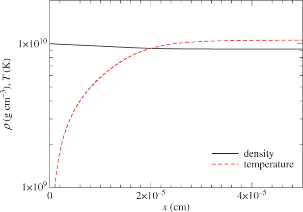
Figure 5. The thermodynamics profile of the deflagration wave with an initial density of 1010 g cm−3 and temperature of 108 K, and a composition of 50% 16O and 50% 20Ne.
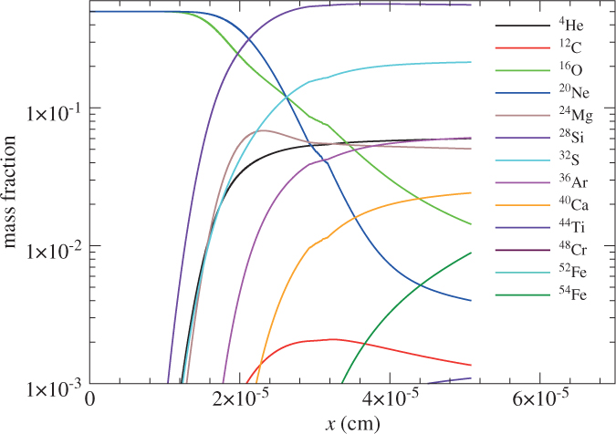
Figure 6. Same as Figure 5 but for the chemical profile.
In Timmes & Woosley (Reference Timmes and Woosley1992), the CO flame and ONe flame are studied systematically for different density under different nuclear reaction networks. The ONeMg laminar flame speed can be approximated by
 \begin{equation}
v_{{\rm cond}} = 51.8~{\rm km ~s^{-1}} \left( \frac{\rho}{6 \times 10^9~{\rm g ~cm^{-3}}} \right)^{1.06}
\left[ \frac{X(^{16}O)}{0.6} \right]^{0.688}.
\end{equation}
\begin{equation}
v_{{\rm cond}} = 51.8~{\rm km ~s^{-1}} \left( \frac{\rho}{6 \times 10^9~{\rm g ~cm^{-3}}} \right)^{1.06}
\left[ \frac{X(^{16}O)}{0.6} \right]^{0.688}.
\end{equation}
4.6.2 Flame Capturing Scheme
In Section 4.6.1, we have described how to analyse the structure of laminar flames through solving the eigenvalue problem of the steady state approximation of the Euler equations. Here, we describe how we model nuclear flames in full-star simulations for the ONeMg core. We have shown that the typical ONeMg flame has a width about 10−5 cm. This is certainly far too small for any modern computer to resolve. This also means that we cannot model flame propagation by only patching the nuclear reactions as an energy source to the system by simply including the nuclear reaction network.
Let us examine the shortcoming of this direct implementation. Consider a zone which is partially burnt by the deflagration. Let the volume burnt (not yet burnt) by the flame is α (1 – α). In hydrodynamics, one has unique density, temperature, and composition for each mesh. However, the thinness of the flame suggests that the actual mesh should be described by two set of quantities, by assigning thermodynamics quantities individually for the ash and fuel, such as Ta, ρa and Xa for the ash and Tf, ρf and Xf for the fuel. The quantities updated by the Euler equations are only some average of these two set of quantities. Therefore, if we solve the nuclear reaction by directly using the original ρ, T and X, we are incorrectly assuming that all the fuel is burning. Notice that laminar flame has a propagation much slower than the speed of sound. In typical explicit hydrodynamics code where the timestep is limited by the Courant–Friedrich–Levy criteria, the flame in each step can propagate at most a distance of v condΔt = (v cond/vs)Δx ∼ 10−2Δx. This suggests that all the fuel is completely burn after ∼102 steps. This simple approach overestimates the fuel consumption rate.
One can imagine to solve for the two set of variables. Then during the simulation, after the hydrodynamics phase, we obtain the averaged quantities Ts, ρs and Xs which represented the mass averaged quantities from the fuel and ash. Using the conservation of mass, momentum, and energy, we have
 \begin{eqnarray}\alpha \rho_a + (1 - \alpha) \rho_f = \rho_s,\end{eqnarray}
 \begin{eqnarray}\alpha \epsilon_a + (1 - \alpha) \epsilon_f = \epsilon_s,\end{eqnarray}
 \begin{eqnarray}\alpha \textbf{X}_a + (1 - \alpha) \textbf{X}_f = \textbf{X}_s.\end{eqnarray}
Hence, one first solves for ρf, ϵf and Xf and then recovers Tf accordingly. This is possible when the ash properties, if assuming complete burnt, can be analytically known. However, as indicated in Reinecke et al. (Reference Reinecke, Hillebrandt, Niemeyer, Klein and Gröbl1999a), such decomposition is physically consistent but numerically difficult because numerical noise owing to discretisation or numerical residue left from the decomposition can make the root-finding impossible. In particular, in multidimensional simulations where Eulerian hydrodynamics is used, the numerical diffusion in the advection scheme always causes mixing with neighbouring meshes. Such additional mixture, which is a source of numerical noises, strongly contaminates the original local information of the fuel and ash. Furthermore, in the case of using realistic EOS table, the root finder scheme is also limited by the interpolation accuracy of the table. Therefore, albeit being the most self-consistent approach in modelling the fuel-ash difference, such approach is seldom applied.
To resolve this difficulty, three approaches are commonly used. In general, they introduce new quantities that represent the flame geometry. They include the level-set method, the point-set method, and the advective–diffusive–reactive flame method.
The level-set method introduces a scalar field S, which is similar to other scalar quantities like the density or electron fraction, which can be transported by the fluid. The scalar field can always be evolved by itself. The scalar field represents the minimal distance of the point of the field to the surface of interest, in our case, the ONe deflagration front. Thus, it satisfies the properties |∇S| = 1. The evolution of S can be written as
 \begin{equation}
\frac{\partial S}{\partial t} + \textbf{\textit{v}} \cdot \nabla S = -\textbf{\textit{v}}_f \cdot \nabla S.
\end{equation}
\begin{equation}
\frac{\partial S}{\partial t} + \textbf{\textit{v}} \cdot \nabla S = -\textbf{\textit{v}}_f \cdot \nabla S.
\end{equation}
The flame surface is defined by the zero contour of the field S. Since the flame propagates in the normal direction, we have vf ⋅ ∇S = v cond∇S ⋅ ∇S = v cond if the distance property is satisfied. This is however not true in general. For a laminar flow, the structure of the flame can be preserved that there is no topological change. But in a turbulent flow, we expect the eddies to continuously disturb the flame surface, which creates complicated structure by smearing or even detaching part of the flame from the main structure. In that case, the topological change of the flame makes the distance properties breakdown. In order to recover this properties, a re-initialisation step is necessary (Sussman, Smereka, & Osher Reference Sussman, Smereka and Osher1994). After updating the scalar field S, the flame surface is obtained, denoted by points xflame,i, where i = 1, 2,…, then all the values of S are recalculated according to the formula:
 \begin{equation}
S_{{\rm new}}(\textbf{x}_j) = S_{{\rm old}} \delta (d_{j}) + {\rm sign}(S_{{\rm old}}) d_{j} \left[ 1 - \delta (d_{j}) \right].
\end{equation}
\begin{equation}
S_{{\rm new}}(\textbf{x}_j) = S_{{\rm old}} \delta (d_{j}) + {\rm sign}(S_{{\rm old}}) d_{j} \left[ 1 - \delta (d_{j}) \right].
\end{equation}
Here, dj is the distance of the mesh to the flame surface dj = mini|(xflame,i −xj)|, δ(x) is a function satisfying δ(x) = 0 when x → ∞, and δ(x) = 1 when x = 0. This function is to give a weight to the correction that points near the flame surface are not changed, so that the flame position, which should not depend on the representation, remains unchanged throughout the operation. The sign function guarantees that the reinitialisation does not change the status of the fuel–ash classification.
The advantage of the level-set method is its easy implementation owing to its scalar property. It can be generalised to simulations to high dimensions. For example, in Reinecke et al. (Reference Reinecke, Hillebrandt and Niemeyer2002b) the level-set method is applied to capture the flame in the three-dimensional Type Ia supernova simulation. Also, the scalar property can handle topological change of the flame straightforwardly. However, the reinitialisation can be time consuming, which scales as Nn +1 for a n-dimensional simulation with N mesh on each dimension. Certain enhancement schemes, such as the narrow band method and the binary-tree method (Sethian Reference Sethian1996, Reference Sethian1999) are proposed to avoid redundant calculations.
The second method is the point-set method (Glimm et al. Reference Glimm, Grove, Li and Zhao1999). In this method, we describe the flame surface by its surface. For simplicity, let us consider the two-dimensional case, where the flame front is characterised by lines. The point-set method makes use of tracer particles to trace the motion of the flame. The geometry of the front is reconstructed by connecting the nearest tracer particles by straight lines. The tracer particles are only pseudo particles that are massless and do not provide feedback to the fluid motion. They only record the position of the flame front. Therefore, the motion of the particles satisfies the equation of motion:
 \begin{equation}\frac{d \textbf{x}_i}{dt} = \textbf{\textit{v}}_i,\end{equation}
where i = 1,2,…,np are the identification number for each particle. The velocity of the particle vi is obtained from the fluid velocity of the Eulerian mesh where the particle locates.
Similar to the level-set method, the point-set method can exactly describe the motion of the surface when the flow is laminar. However, complications can take place when the flow is turbulent. The tracer particles can become too closely or sparsely distributed when the structure is affected by the eddy motion. In that case, particle addition or deletion is necessary to make sure the simulation maintains the required resolution for the flame with an optimal number of particles. In the upper part of Figure 7, we draw the schematic diagram for adding or removing particles which is a common procedure in this method. When the particles become overcrowded (underpopulated), we remove (locate) the concerned particle, and we reconstruct the geometric information of the flame. Another commonly encountered situation is that when two groups of particles approach each other, it is possible that the two particles which are originally regarded as a pair forming the front, is no longer so because there are new neighbouring particles which are even closer. This corresponds to the case when two flame patches merge to one bigger patch, in which topological change of the flame front occurs. To resolve it, one needs to identify the new nearest neighbours by checking the inter-particle distance again and reconnect the lines to build the new flame front by choosing the new nearest neighbour.
Figure 7. Particle insertion, deletion, and line operation for the point-set method.
The advantage of this scheme is that the particle exactly traces the location of the front, which is free from any interpolation scheme. The scheme is also free from numerical diffusion. Therefore, small scale structure induced by hydrodynamics instabilities can be preserved, which can be important for studies where the diffusion process is critical. However, there are two major disadvantages. First, it requires the use of linked set for a convenient operation. This means additional extensive coding is required for an efficient manipulation of the particles. Second, its three-dimensional extension can be non-trivial that it requires a surface to describe the front. For example, in Glimm et al. (Reference Glimm1998, Reference Glimm, Grove, Li and Tan2000), it is proposed to use to represent the front by triangle patches. In the three-dimensional case, there are always degenerate solutions for adding, removing particles, or doing surface operations. This adds uncertainties to the application of fluid flow with frequent topological changes.
The last method which is commonly used in flame capturing is the advective–diffusive–reactive flame (ADR) scheme. This scheme is similar to the level-set method that it introduces a scalar field cf which can propagate by itself and be transport by underlying fluid motion. But it represents the fraction of the ash. When cf = 1, it represents a complete ash and cf = 0 represents a complete fuel. Its evolution satisfies
 \begin{equation}\frac{\partial c_f}{\partial t} + \textbf{\textit{v}} \cdot \nabla c_f = \dot{c}_f + \kappa \nabla^2 c_f.\end{equation}
The two terms on the right-hand side correspond to the reaction and diffusion terms. The reaction term is a simplified representation to the change rate from fuel to ash. In the context of ONeMg core, it can correspond to the burning of 20Ne and 24Mg to NQSE elements, peaked by 28Si. The diffusive term symbolises the propagation of the deflagration front by thermal conductivity. To mimic the propagation of flame, one chooses (Vladimirova, Weirs, & Ryzhik Reference Vladimirova, Weirs and Ryzhik2006)
 \begin{equation}
\dot{c}_f = \frac{f}{4} (\phi - \epsilon_0) (1 - c_f + \epsilon_1),
\end{equation}
\begin{equation}
\dot{c}_f = \frac{f}{4} (\phi - \epsilon_0) (1 - c_f + \epsilon_1),
\end{equation}
where ϵ 0 = ϵ 1 = 10−3, f = 1.309. The presence of ϵ 0 and ϵ 1 provides a truncated reaction rate, which can make the flame front stay localised, and its bistable property gives a unique flame speed (Xin Reference Xin2000). These variables are chosen by experience so as to minimise the numerical noise, which frequently appears when fuel is depleted. The diffusion term is given by
 \begin{equation}\kappa = \frac{1}{16} s b \delta_x.\end{equation}
s is the laminar flame speed obtained from direct flame calculation (See Section 4.6.1 for the physical meaning). b= 3.2 is the number of zones for the diffusion.
This method shares similar virtue as the level-set method that it can be easily implemented and can be easily generalised to higher dimensional cases. However, in applications one needs to configure the reaction and diffusion terms in order to make the model to manifest the deflagration wave with the expected rate and speed. Also, one should pay extra attention to the discretisation scheme. A naive discretisation can lead to amplification of acoustic noise, which may wrongly enhance the diffusion and thus the reaction.
We have described how one can capture the motion of deflagration through the use of tracer particles including the level-set method, point-set method, and the ADR scheme. In the simulations, one solves the evolution of those quantities (S for the level-set method, particle positions for the point-set method, and so on) introduced in these schemes, together with the hydrodynamics. Then, we reconstruct the structure of the flame based on the information of those quantities. By comparing the geometry before and after the update, one obtains the area or volume swept by the flame in that time step. Then, the amount of energy and change of composition can be applied to the meshes.
4.6.3 Deflagration–detonation transition?
In the late time of the explosion for the ECSN which could undergo a direct explosion, the flame can reach some low-density regions, where the deflagration slows down and the flame is thickened by the turbulent diffusion near the flame surface. For the CO case, the flame is halted and the carbon burning ceased. The eddy motion near the flame surface becomes important that it continues to diffuse thermal energy from the hot ash and distributes to the surrounding fuel. At a certain point, a non-local area reaches the temperature for explosive carbon burning. Then the detonation spot is triggered. This is known as the Zel’dovich gradient mechanism. To determine whether the turbulence is sufficiently efficient to take away the heat generated by the nuclear reaction, the Karloritz number Ka is frequently used, which is defined by Ka = τ turb/τ flame. For Ka < 1, turbulence is too slow to take away energy from the deflagration boundary, or the nuclear reaction is rapid enough to generate energy to support the propagation. This happens during the early time of explosion or when the flame front is around the stellar core. For Ka ≥ 1, the eddy motion near the flame surface is sufficiently fast to remove the additional heat generated by the deflagration front, or the nuclear reactions slow down as a result of decreasing density. The latter case is often treated as the necessary condition for the start of the detonation.
It has been a concern whether or not the deflagration–detonation transition may be triggered in thermonuclear runaway. In the scenario of Type Ia supernova, such transition is important as it allows most matter in the CO white dwarf to be completely burnt, which may provide adequate energy to disrupt the star. Also, such feature can compensate the shortcoming of the (turbulent) deflagration, which propagates in the diffusion timescale, to produce the very high velocity intermediate mass elements to explain the observed feature. Early one-dimensional work, such as Khokhlov (Reference Khokhlov1991a, Reference Khokhlov1991b), the deflagration–detonation transition is treated as a model parameter. However, whether such a transition is physically possible is in doubt by later dimensional estimations (Niemeyer & Woosley Reference Niemeyer and Woosley1997; Lisewski, Hillebrandt, & Woosley Reference Lisewski, Hillebrandt and Woosley2000) and by the linear-eddy model (Woosley et al. Reference Woosley, Kerstein, Sankaran, Aspden and Roepke2009). This is because to trigger the detonation, the flame should enter the distributed regime, where turbulence should act as an inhibitor of the flame propagation by diffusing the heat generated by nuclear reaction to the fuel. Such condition has led to a stringent requirement in the turbulence strength.
5. Electron-degenerate ONeMg cores
We have described the physics contributing to the evolution of an electron-degenerate ONeMg core in the deflagration phase in details. In this section, the physics and technique are described for hydrodynamical simulations of the ONeMg core. First, we describe the hydrodynamics and energetics of typical ONeMg core models. Then, we examine how the uncertainties in stellar evolution influence the final fate of the ONeMg core. These uncertainties come from different origins, including for example the one-dimensional spherical assumption in the stellar evolution models and the use of parametrisation schemes. As a result, we consider the variations in the central density, initial flame structure, and the input physics.
In the evolution of ONeMg cores, we encounter the following uncertainties. First, it is the semi-convection associated with electron captures. Depending on the efficiency of semi-convection, the ONe-deflagration density in the ONeMg can change from ∼1010.2 (Schwarzschild criterion) down to ∼109.95 g cm−3 (Ledoux criterion). Semi-convection is an over-stable convection, so that the oscillatory convective instability and the associated mixing grow with the timescale of heat-exchange. More mixing leads to a higher central density (Takahashi et al. Reference Takahashi, Yoshida and Umeda2013). Therefore, 109.95 g cm−3 set by the Ledoux-criterion is the lower limit to the deflagration density. In the present case, electron capture forms the extremely steep gradients in both temperature and Ye, so that the analysis of semi-convective mixing requires careful possibly multi-dimensional simulations.
The second uncertainty is the initial flame structure. The development of the initial flame is sensitive to the internal motion of the star. However, in stellar evolution, which is modelled in one dimension, the non-radial motion of matter is neglected. In particular, local turbulence can provide velocity and temperature fluctuations, which can be important near the runaway phase. Without an exact knowledge about the internal motion of the star, one cannot derive the exact position of the first nuclear runaway, as well as its possible shape. Therefore, the initial flame of the ONeMg, similar to Type Ia supernova, is poorly constrained.
The third uncertainty is the relativistic effects. The impact of relativistic effects is unclear. In the ONeMg core, the density in the core is high enough that the electrons become relativistic. In that case, the contribution of the pressure and internal energy as a gravity source becomes non-negligible. One has to study how these components contribute to the dynamics, and whether the collapse criteria changes with them.
5.1. Typical models
The typical behaviour of models which show an expansion or a direct collapse is studied here. To contrast the dynamics between these two similar models where one of the models has a central density of 109.95 g cm−3 (i.e., 8.91 × 10⁹ g cm−3) and the other one of 109.925 g cm−3 (i.e., 8.41 × 10⁹ g cm−3). To demonstrate the sensitivity to the runaway density of the typical ECSN model, the initial flame used here is slightly more massive than those in Section 5.2. Other input physics and initial flame are fixed for a consistent comparison. The code is based on the two-dimensional hydrodynamics with flame capturing (Leung, Chu, & Lin Reference Leung, Chu and Lin2015a). The code has been applied to various scenarios, such as normal and sub-luminous Type Ia supernovae of Chandrasekhar mass white dwarf (Leung, Chu, & Lin Reference Leung, Chu and Lin2015b; Leung & Nomoto Reference Leung and Nomoto2018), AIC models (S.-C. Leung et al. Reference Leung and Nomoto2018, in preparation), and the deflagration phase of ONeMg core (S.-C. Leung and K. Nomoto 2018, in preparation).
5.1.1. Central density and Ye
In Figure 8, we plot the central density against time for the two models. In both models, the central density mildly increases in the first 0.2 s. However, after 0.2 s, the evolution of the two models deviates from each other. For the collapsing model, after 0.2 s, the increment in density resumes again. The process accelerates and the central density reaches as high as 1011 g cm−3 at 0.55 s. This shows that the core-collapse is proceeding. For the exploding model, the central density remains steady for about 0.5 s, and then it drops gradually. Its density drops to 1% of its initial value at about 1 s after the trigger of deflagration. This shows that the expansion starts.
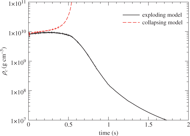
Figure 8. The central density against time for two contrasting models.
We first note the existence of a hierarchy in the timescale, the strong interaction (in particular NSE timescale) t NSE, the weak interaction timescale t weak, and the hydrodynamical timescale t hyd. For ONeMg core, we have t NSE ≪ t hyd < t weak in the core with a typical density 1010 g cm−3 and a temperature 1010 K. As a result, the matter composition is almost simultaneously adjusted according to local (ρ, T, Ye). The highly relativistic and degenerate electron gas has an adiabatic index Γ ≈ 4/3. Furthermore, the photo-disintegration of 56Ni into 4He or recombination of 4He into 56Ni further lowers the effective Γ.
In Figure 9, we plot the change in the central Ye. As in the central density (Figure 8), Ye of both models show similar evolution; they decrease quickly from 0.5 to 0.4 by electron capture.
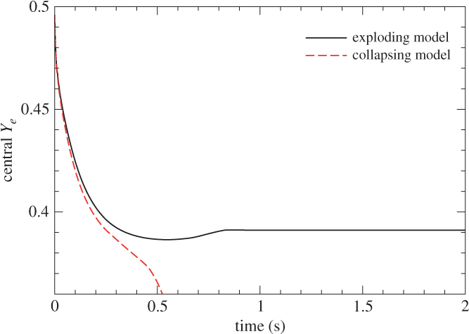
Figure 9. Similar to Figure 8 but for the central electron fraction Ye.
These figures show that electron capture on NSE materials tends to induce contraction of the core by lowering Ye. On the other hand, nuclear energy release due to ONe-deflagration tends to induce expansion of the core. In the present model, electron capture is slow so that these competing processes occur in almost hydrostatic equilibrium, and the outcome depends mostly on the central density.
It should be noted that the trigger of the collapse is very different from the Fe-core collapse. In the Fe-core, the softening of core comes from photo-disintegration, which occurs in NSE timescale, thus the whole process is dynamical. While in ECSN, the softening process depends on the weak interaction, the drop of adiabatic index Γ is determined by t weak, and therefore the whole process is quasi-static.
5.1.2. Energy production
In Figure 10, we plot the luminosity for the ONe deflagration, advanced burning, neutrino luminosity, and total energy change rate from all these reactions. Here, we call ONe deflagration for the explosive ONe burning to realise NSE with the timescale of temperature rise (τ rise) being shorter than the dynamical timescale (τ dyn). We include in the upper panel the collapsing model and in the lower panel the exploding model. The energy change rate is defined by ΔQi/Δt, where Δt is the current time step, and ΔQi is the energy released by channel i in the simulation, where i can be ONe deflagration, advanced burning, and energy loss by neutrino. In general, the ONe deflagration and advanced burning are almost simultaneous so that they may belong to one single luminosity. The timescale for a complete burning is much shorter than the local time step. Here, we separate the two components to present their corresponding energetics components.
For the collapsing model, the nuclear reactions are less important to the whole energy production. Instead, the neutrino emission dominates the total luminosity. As the core begins to collapse, the neutrino luminosity grows with time.
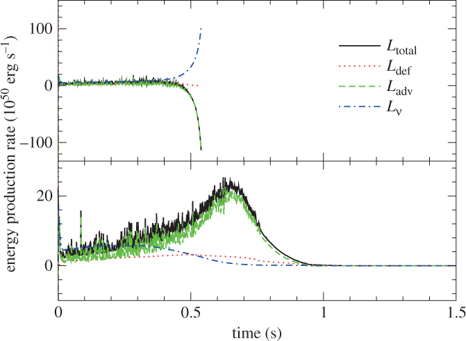
Figure 10. Similar to Figure 8 but for the total luminosity, luminosity from ONe deflagration, luminosity from advanced and NSE burning, and energy loss rate by neutrino emission. We show the collapsing (exploding) model in the upper (lower) panel.
In the exploding model, the nuclear energy production rate is similar to the Type Ia supernovae in the pure turbulent deflagration scenario. The energy production is slow at the beginning, because the flow is not yet turbulent to accelerate the flame propagation. At about t = 0.5 s, the energy production rate is the fastest, showing that the flame is most enhanced by turbulence acceleration. Then the luminosity gradually drops and reaches zero about t = 1 s, showing that the fuel density outside the flame drops and the flame quenches. By comparing the ONe deflagration and advanced burning, we can see that the ONe deflagration releases only part of the energy in the full reactions. Most of the energy comes from advanced burning, i.e., the recombination energy mainly from 4He to 56Ni. The neutrino luminosity, on the other hand, is lower than the energy production rate from nuclear reactions. It reaches its maximum earlier at t = 0.3 s and then slowly drops.
5.1.3. Energetics
In Figure 11, we plot the total energy, kinetic energy, internal energy, and net gravitational energy of the collapsing (exploding) model in the upper (lower) panel.
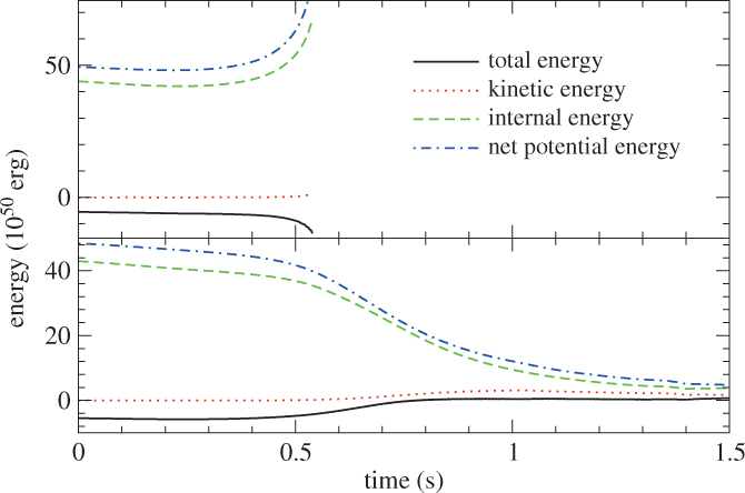
Figure 11. Similar to Figure 8 but for the total energy, kinetic energy, internal energy, and net gravitational energy for the collapsing (exploding) model in the upper (lower) panel.
For the collapsing model, again the total energy is negative initially owing to the initial setting. However, there is no increase in the total energy throughout the simulation. It continues to drop and the contraction accelerates after 0.5 s, showing that the system cannot gain energy by nuclear reactions. The kinetic energy shows a similar pattern but with a different direction. The total kinetic energy is almost zero for the 0.5 s, showing that no global motion is induced by the initial flame. However, once the collapse is triggered in the core, the kinetic energy quickly rises. On the other hand, the internal energy and net gravitational energy drop at the beginning, this means the core attempts to reach a new equilibrium by expansion. After 0.3 s, both energies increase again, showing that the star contracts, which compresses the matter in the core and creates a deeper gravitational well.
In the exploding model, the initial system is bounded that total energy is negative ∼ −6 × 1050 erg. The deflagration produces energy and makes the total energy slightly above zero at 0.8 s. After that, it reaches a constant after the deflagration is quenched. The kinetic energy at the beginning is zero, since we construct a static star at the first place. After the deflagration phase, the hot matter pushes the envelope matter outwards, transferring the internal energy to kinetic energy. But when the star expands, the matter decelerates when moving against the gravitational gradient. Thus the kinetic energy drops. The gravitational energy shows a similar evolution. At the beginning, where there is no global movement inside the core, it remains a constant. When the deflagration resumes, the star starts to expand, and hence we see a faster drop in the potential energy. The internal energy also shows a similar behaviour that it is steady for the first 0.5 s. After that, the deflagration resumes its propagation and the star expands. The expansion allows the conversion of internal energy into kinetic energy and then used as work done against gravity.
5.1.4. Flame structure
In Figures 12 and 13, we plot the temperature colour plots of both models at 1.125 and 0.55 s after we start the ONe deflagration. For the exploding model, the flame releases sufficient energy to make the star expand. The original three-‘finger’ structure has evolved to a two-‘finger’ structure, where the middle one is suppressed. Through expansion, the central temperature drops from its peak at 1010 K to 3 × 10⁹ K. The flame has well developed similar to the Type Ia supernovae where signatures of hydrodynamics instabilities can be clearly seen. On the top of flame around 3 000 km from the core, one can see the spiral shapes triggered by the Kelvin–Helmholtz instabilities, namely the mixing between the fuel and ash flowing in the opposite direction. Also, along the diagonal direction one can see an inverse mushroom shape (the blue zone about 1 000 km from the core). It is the Rayleigh–Taylor instability made by the downward falling cold fuel and the upper rising hot ash, owing to buoyancy effects. There is a mildly heated zone of temperature 2 × 10⁹ K near the outer boundary. This is the excited atmosphere owing to the compression by the flame. On the other hand, the flame structure for the collapsing model has much less features than the previous one. The size of flame is about 400 km in size. Owing to the sub-sonic propagation of the flame, the star expands quietly without exciting shock inside the star. Most part of the star remains cold, and there is a mildly hotter envelope from 800 to 1200 km in radius. The infalling matter along the diagonal direction suppresses the development of the middle ‘finger’ compared to the other two. The innermost core about 100 km in radius has a typical temperature of 8 × 10⁹ K, which is slightly colder than the inner envelope of radius 100–200 km. The central core has experienced rapid endothermic electron captures after the ash is formed. This drenches away the internal energy from the core.
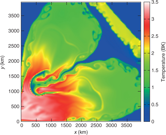
Figure 12. The temperature colour plot and the flame contour for the model showing an expansion at 1.125 s after the trigger of deflagration.
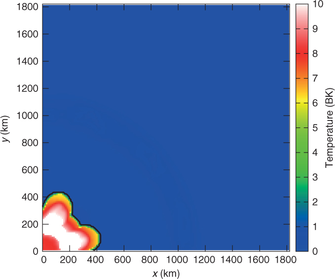
Figure 13. Similar to Figure 12, but for the model showing a direct collapse at 0.55 s after the trigger of deflagration.
5.2. Effects of central density
The typical density for the ONeMg core to runaway is ∼109.95 g cm−3. It should be noted that the exact value is unclear. It is influenced by many processes in the stellar evolution, where many of these are inherently multi-dimensional processes but parametrised models are frequently used.
The pre-ONe deflagration phase is sensitive to how semi-convection is modelled. The central density can reach as high as 1010.2 g cm−3 before the deflagration starts. On the other hand, in Miyaji & Nomoto (Reference Nomoto1987), Hashimoto et al. (Reference Hashimoto, Iwamoto and Nomoto1993), Jones et al. (Reference Jones2013), and Schwab et al. (Reference Schwab, Quataert and Bildsten2015), where semi-convection is not modelled, the runaway density drops to ∼109.95 g cm−3 (see Figure 14). As a result, to constrain the final fate of the ONeMg core, a survey in the models in different runaway density becomes necessary.
Figure 14. The central temperature against central density in log scale of the 8.8 M⊙ star (Hashimoto et al. Reference Hashimoto, Iwamoto and Nomoto1993).
In Figure 15, the central densities against time are plotted for ONeMg models with initial central densities from 109.8 to 1010.2 g cm−3. For a consistent comparison, all models share an identical initial flame of the c3 shape in the core (Reinecke, Hillebrandt, & Niemeyer Reference Reinecke, Hillebrandt and Niemeyer1999b). The c3 flame is a flame located at the corner with three finger shaped extension to mimic the behaviour of Rayleigh Taylor instabilities coming from the initial perturbations of the fluid flow. The initial ash mass is ∼ 10−2M⊙. Models with central densities below 109.90 g cm−3 all show a successful explosion. The central density continuously decreases with time. On the other hand, for models with an initial central density above 109.90 g cm−3, the central densities increase monotonically with time. They are the models which directly collapse to form NSs.
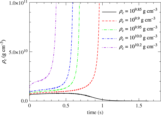
Figure 15. The central density against time for ONeMg models with different central densities. All models start with a central ignition kernel.
5.3. Effects of flame structure
How the flame starts in the ONeMg core during the runaway is highly unclear. In the growing ONeMg core, the capture of electrons on 20O and 24Mg emits high energy gamma-rays, which heats up the surrounding matter. This process determines the initial size of the runaway regime. However, the actual size depends on parameterised processes, such as semi-convection, convective URCA process, and the growth rate of the ONeMg core mass. The semi-convection becomes important during electron capture in the core. Electron capture creates a mean molecular weight difference between the core with a lower Ye and the envelope which remain unchanged. Depending on the efficiency of the semi-convection, the runaway size may vary. In general, efficient semi-convection leads to a faster transport of heat produced during electron capture. Also mixing leads to a wider region with low Ye, which promotes contraction. As a result, the core reaches a higher central density before the temperature becomes high.
We emphasise that uncertainties of semi-convection imply that 109.95 g cm−3 given by Ledoux criterion (i.e., completely no mixing) is the lower limit. URCA shell cooling is important to cool down the core and leads to the higher deflagration density.
These uncertainties make the exact central density and temperature at which the deflagration takes place inconclusive, although a higher deflagration density is indicated. Different flame structure should be tested, to exhaust different possibilities where the flame may appear. This includes varying the position of the flame and the size of the flame.
In Figure 16, we plot the central density against time for the ONeMg core at the same central density 109.95 g cm−3 but with the initial flame at different position. The flame varies from at the centre, at 50, and 100 km from the core. This mimics the effects where the flame is being transported by the global convective motion before the hot spot of the electron capture zone enters runaway temperature. It can be seen that the model where the flame located at centre collapses into an NS while the flame located off-centre explodes. This shows that the geometric effects of the flame can be important to the final fate of ECSN.
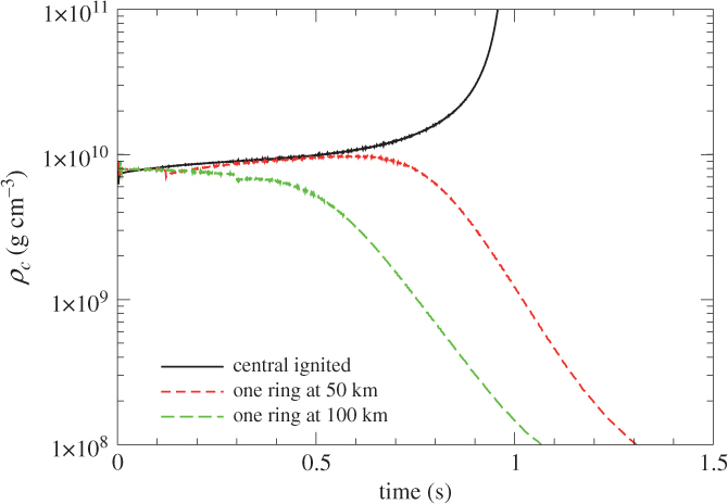
Figure 16. The central density against time for ONeMg models with different flame structure. All models start with a central density 109.95 g cm−3.
We remind that in two-dimensional simulations, the off-axis bubble corresponds to a ring in the three-dimensional projection. To form this flame, an environment with rotation symmetry is required. For a more general flame structure, we refer to Jones et al. (Reference Jones, Röpke, Pakmor, Seitenzahl, Ohlmann and Edelmann2016). In that work, the growth of deflagration is studied by three-dimensional simulations. The three-dimensional simulation allows more realistic modelling of bubbles. It starts with ∼100 runaway bubbles as the initial condition. However, it is unclear whether the multi-spot runaway can be triggered naturally.
In Figure 17, the central density against time for the ONeMg core is plotted at the same central density 109.95 g cm−3 and with a central ignition kernel but with different size. Flame with an inital mass from ∼10−4 to 10−2M⊙ is used. It can be seen that model with a small flame collapses while that with a large flame expands. The models with initial flame masses 10−4 and 10−3 M⊙ collapse while the model with that of 10−2M⊙ expands. This also suggests that the runaway size can determine whether the final fate of ECSN. Notice that the collapse time is also related to the initial flame size. A larger runaway size leads to a faster collapse. It is because the larger initial ash provides a larger volume for electron capture, which enhances the infalling flow of matter at the beginning.
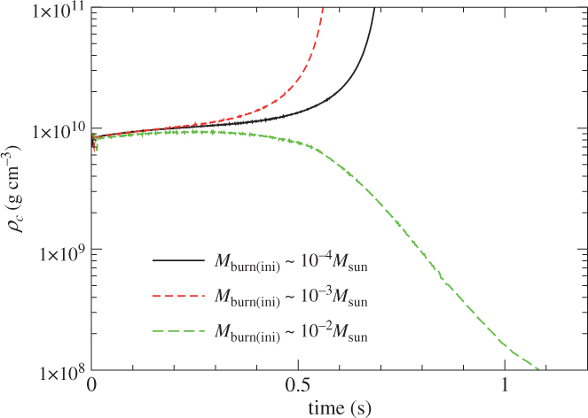
Figure 17. The central density against time for ONeMg models with flame size. All models start with a central density 109.95 g cm−3 and the flame starts at the centre.
We note that the initial size of the flame depends also on the laminar phase. But to simulate the laminar flame, the initial runaway mass must be small. Smaller burnt mass corresponds to longer laminar phase. Larger burned mass means that the mass is burnt very quickly, or faster flame, which is less likely. Again to resolve the laminar phase, with the ONe-deflagration has just started, the required resolution (∼cm) is beyond current computation capability.
By considering the two tests, it can be seen that the size of the flame and its initial position are the two important parameters which determine the final fate of the ONeMg core. This means, the current ECSN models discussed here show a tendency that the collapse follows after nuclear deflagration in the ONeMg core. The diversity of the final results means more detailed studies, including extension to three-dimensional simulations, are needed.
5.4. Effects of input physics
5.4.1. Flame physics
One important uncertainty in modelling the ONeMg core is the turbulent flame prescription. In the literature, sub-grid turbulence models are always approximate models to mimic the statistical behaviour of velocity fluctuations inside the Eulerian mesh. Uncertainties exist from the choices of closure relations and phenomenological fitting of these models. This can also affect the collapse/explosion conditions. To demonstrate the importance of the turbulence model, recall the flame speed formula:
 \begin{equation}v_{{\rm flame}} = v_{{\rm lam}} \sqrt{1 + C_T \left( \frac{v'}{v_{{\rm lam}}} \right) }.\end{equation}
The constant CT is a free parameter. It is chosen to be CT 0 = 4/3 for the turbulent flame in the terrestrial experiments. However, it is unclear whether the flame in the ONeMg core behaves similarly as the terrestrial flame, owing to the qualitative difference of the energy-release mechanism and the huge difference in the hydrodynamics constants, such as the Rayleigh’s Number.
To understand the effects of the turbulence–flame interactions, the evolution of the ONeMg core with a parameterised flame speed is studied. In particular, other choices of CT, CT 0/2 and CT 0/4 are used. In Figure 18, the central densities of the ONeMg cores are plotted. All models show a direct collapse. The model collapses faster when the effective propagation speed is high. For example, the model with only a quarter of the original flame speed is ∼50 ms slower to start collapse than the original model. This is because the faster the deflagration is, the faster the ash is formed in the star, which further contributes to the contraction–electron capture cycle.
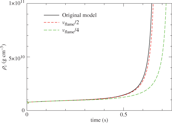
Figure 18. The central density against time for ONeMg models with different flame propagation speed. 100%, 50%, and 25% of the original values are used. All models begin with a c3 flame and a central density 109.925 g cm−3.
5.4.2. General relativistic effects
The last input physics examined here is the relativistic contribution as a gravity source. In all models considered, the electron gas is ultra-relativistic and degenerate. We remind that the Fermi energy of the ideal degenerate Fermi gas at zero temperature is given by E Fermi = (3π 2ℏ 3n)(1/3), with n being the particle number density. This suggests that the energy of the system can be non-negligible when compared with the rest-mass of the electron gas.
To estimate the mass-energy contribution of the electron gas as the gravity source, the TOV extension is used (Kim et al. Reference Kim, Kim, Choptuik and Lee2012). In this formalism, the Poisson equations describing the Newtonian gravity is modified as
 \begin{equation} 4 \pi G \nabla^2 \Phi = \rho_{{\rm active}},\end{equation}
where
 \begin{equation} \rho_{{\rm active}} = \rho h \frac{1 + v^2}{1 - v^2} + 2 P,\end{equation}
where P and v 2 are the fluid pressure and the magnitude square of the velocity, respectively. h = 1 + ϵ + P/ρ is the specific enthalpy of the matter. In this sense, the extra mass-energy owing to the internal energy and the kinematic of the matter are included. In this approximation, all energy of the fluid is included. However, the gravitational energy generated by the self-gravity is not included. In fact this term is still small in comparison. For a typical ONeMg core, M = 1.4 M⊙ and R = 1000 km. This gives, in geometric units (G = c = 1) where M⊙ = 1, the self-gravitational energy as E grav ∼ 10−3. The corresponding energy density can be estimated as
 \begin{equation}
\epsilon_{{\rm grav}} = \frac{E_{{\rm grav}}}{V} \approx \frac{M^2}{R^4}\ {\sim} \frac{\rho M}{R}.
\end{equation}
\begin{equation}
\epsilon_{{\rm grav}} = \frac{E_{{\rm grav}}}{V} \approx \frac{M^2}{R^4}\ {\sim} \frac{\rho M}{R}.
\end{equation}
Assuming this energy contributes also to the gravity, the effective ρ active would be qualitatively modified as
 \begin{equation}
\rho_{{\rm active}} = \rho h \frac{1 + v^2}{1 - v^2} + 2 P + \epsilon_{{\rm grav}}.
\end{equation}
\begin{equation}
\rho_{{\rm active}} = \rho h \frac{1 + v^2}{1 - v^2} + 2 P + \epsilon_{{\rm grav}}.
\end{equation}
Typical P ∼ ϵ ∼ 10−2ρ. The gravitational self-energy is of one order of magnitude smaller, and hence we neglect its contribution in this approximation. However, for neutron stars, this correction will be important.
ONeMg core models at the high end of initial central densities are studied. In these models, relativistic effects are the most pronounced. In Figure 19, we plot the central densities of the ONeMg models with a central density of 1010 and 1010.2 g cm−3, respectively. All models are set to share identical flame structure of the c3 flame and with the same ash mass. By comparing models with the same initial central density, it can be seen that the two curves overlap with each other. This suggests that even the electron is ultra relativistic, it remains a good approximation to use Newtonian gravity for modelling ECSN.
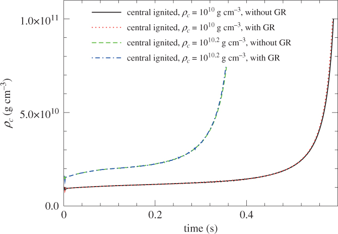
Figure 19 The central density against time for ONeMg models with or without the relativistic effects. Models are set to have a central density of 1010 and 1010.2 g cm−3 and with a centred ignition kernel.
5.5. The directly expanding case
In this subsection, we discuss the different outcome that the ECSN progenitor can have, i.e., the ONeMg core does not directly collapse into an NS but expands, depending on their runaway density, runaway position and the exact input physics. If this would be the case, it would behave like a weakly exploding Type Ia supernova.
After the expansion starts, the core matter quickly cools down and the density drops. Then the ONe-deflagration quenched as it can no longer supply sufficient energy for sustaining its propagation. Such directly expanding models have also been observed in the multi-dimensional simulations of the ECSN runaway phase (Jones et al. Reference Jones, Röpke, Pakmor, Seitenzahl, Ohlmann and Edelmann2016), where the multiple off-centre flame bubbles are placed in the ONeMg core as the initial runaway trigger. Due to the much more extensive distribution of bubbles in their work, they observe that about a half of the white dwarf is ejected, which makes its total mass lower than the Chandrasekhar mass. Unlike the classical one-dimensional model for Type Ia supernovae, where ejecta shows a stratified composition, the turbulent nature provides such a strong mixing in the ejecta that a comparable amount of Fe-peak elements can be found in both the remnant and ejecta. This is because when the hot ash is expanding and rising after burnt, the hydrodynamical instabilities provide the necessary mixing to the surrounding fuels and also take away part of its momentum. Part of the hot ash is then trapped by the white dwarf. It falls back and forms the remnant.
5.6. A short summary of this section
We have presented some comparative study of the evolution of the ONeMg core under different central densities, flame structure and flame size, and the input physics. For the classical model of an ONeMg core which starts the ONe deflagration at a central density ≈ 109.95 g cm−3, the core can successfully collapse into a neutron star without creating a low-energy explosion. We have also shown the sensitivity of the collapse condition on the initial central density, flame structure, and flame size. This suggests that a precise condition that the ONe deflagration starts is important. This includes the heating effects of electron capture by 20Ne and 24Mg that releases gamma-rays, and the deflagration position, which is determined by the pre-deflagration convective motion in the central region. In particular, the turbulent fluid motion is vital for the heated fluid parcel since the exact deflagration position is a competition between the adiabatic expansion of the hot fluid parcel and the slow nuclear burning in the pre-deflagration convective region. Note whether such a slow nuclear burning phase exists depend on the convective criterion. As seen in Figure 14 where the Ledoux criterion is applied, ONe burning is already rapid enough to become a deflagration when the convective motion starts under the Ledoux criterion. This suggests that an accurate prescription of the many processes in stellar evolution, such as semi-convection and convection, are necessary.
6. Extension to CO and CONe white dwarfs
6.1. Nuclear runaway of CO white dwarfs
The composition of CO WDs is a matter of debate, because it involves the nuclear reaction 12C(α, γ)16O, which is not well constrained. Also, the composition is known to be sensitive to how the convective mixing and overshoot is modelled, while so far only local theory of these physical processes is present. In Umeda et al. (Reference Umeda, Nomoto, Yamaoka and Wanajo1999), the metallicity and mass dependence of the C/O mass fraction ratio in the white dwarf are explored. The typical range of C/O ratio is between 0.3 and 0.6. The ratio is smaller for lower mass white dwarf, and it increases until the main-sequence star mass is about 4–5 M⊙. Then it slowly decreases.
In the close binary systems, the mass transfer to the companion star produces similar low mass CO white dwarfs. In close binaries, mass accretion from the companion star of the white dwarf, such as a slightly evolved main-sequence star and a red giant with an extended hydrogen envelope, becomes critical. In Nomoto et al. (Reference Nomoto, Thielemann and Yokoi1984), this phase is modelled and it is shown that whether the accretion leads to a Type Ia supernova depends on both the initial mass of the WD and the accretion rate (See also Kawai et al. Reference Kawai, Saio and Nomoto1988 for the extension to He- and C-accretion). It is also possible that such star undergoes a direct collapse, similar to the ONeMg white dwarf, depending on the parameters. Therefore, it becomes necessary to extend the calculation to CO white dwarfs.
The preparation of the model is similar that one constructs a CO white dwarf in hydrostatic equilibrium at a pre-determined density. The initial CO flame is put in by hand in the white dwarf to trigger the C-deflagration phase. The hydrodynamics, together with the explosive nuclear reactions and the energy loss by neutrino emission, is tracked.
In Figure 20, we plot the central density against time for the CO white dwarf models with a central density from 109.90 to 1010.2 g cm−3. All models have the same centred ignition kernel and the same composition at C/O = 1. It can be seen that models with a central density below 109.975 g cm−3 explode, while those above that collapses. Similar to the ONeMg WD, the higher density leads to a faster collapse. The behaviour shows that in this density range the fate of the CO white dwarf is also sensitive to the initial density, and the CO white dwarf requires a higher central density for the collapse to occur than ONeMg cores. This is because the CO fuel releases more energy than the ONeMg fuel at the same density.
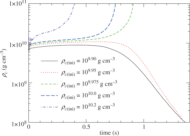
Figure 20. The central density against time for CO models are set to have a central density from 109.90 to 1010.2 g cm−3 and with a centred ignition kernel with an initial mass ∼ 10−4M⊙.
The evolution of CO white dwarfs for the different C/O ratio is shown in Figure 21. All models are prepared with the same central density of 109.95 g cm−3 and with a central ignition kernel of the same mass. Models with the C/O ratio from 0.25 to 0.50 directly collapse into a neutron star while that above 0.50 directly explodes as a weak Type Ia supernova. The lower the initial C/O ratio the star has, the faster is the collapse. Similarly, when the C/O ratio becomes higher, the explosion is stronger with a faster expansion of the white dwarf. This further adds the importance of a consistent stellar evolution in order to predict the initial C/O ratio of the progenitor model (Benvenuto et al. Reference Benvenuto, Panei, Nomoto, Kitamura and Hachisu2015). As shown in Umeda et al. (Reference Umeda, Nomoto, Yamaoka and Wanajo1999), metallicity plays an important role in the final C/O ratio prior to the explosion to take place.
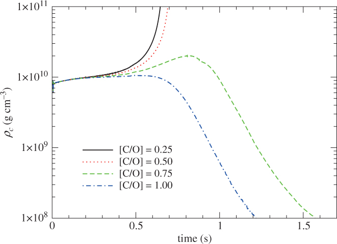
Figure 21. The central density against time for CO models are set to have a central density from 109.95 and with a centred ignition kernel, but at different C/O ratio including C/O = 0.25, 0.50, 0.75, and 1.00 with an initial ash mass of 10−3M⊙.
In this section, we discussed the effects of central density and C/O ratio for the final evolution of CO white dwarf after the deflagration phase. It can be seen that the importance of the initial model persists even for the CO white dwarf model.
6.2. Explosion of hybrid CO(Ne) cores
In Woosley et al. (Reference Woosley, Heger and Weaver2002), it is shown that near the lower mass end of the super-AGB mass range (∼8M⊙), the off centre burning of carbon may create a two-layer structure, a core with C and O and an envelope with O and Ne. Whether the C-flame can reach the core is a matter of debate due to these two factors. First, it is the competition between heat diffusion and the convective boundary mixing, which prohibits the C-flame from reaching the core by heat conduction (Dominguez, Tornambe, & Isern Reference Dominguez, Tornambe and Isern1993). Second, the neutrino cooling can efficiently take away the thermal energy generated by the slowly propagating C-flame, which stops its propagation.
However, the exact remaining CO mass depends on two theoretical uncertainties, first, the carbon burning rate and second, the strength of the convective boundary mixing. The carbon burning rate can differ by a few orders of magnitude due to the presence of resonance and hindrance in its reaction kernel (Chen et al. Reference Chen, Herwig, Denissenkov and Paxton2014). The convective boundary mixing is numerically difficult in modelling convection by the stellar evolution codes. In the convective cell, the fluid parcel needs not to have a zero velocity when it reaches the convective boundary. But it also quickly loses its momentum when the parcel enters the convectively stable zone. As a result, there is a non-zero mixing between the convective zone and outside the zone. This effect becomes important to the quenching of the C-flame, because it determines how fast the diffusion can remove the heat from the ash. A faster removal of thermal energy means an earlier quenching of the flame (Denissenkov et al. Reference Denissenkov, Herwig, Truran and Paxton2013).
The failed propagation of C-flame can leave a carbon-rich core of mass from 0.2 to 0.45 M⊙, or as high as 0.74 M⊙, if the full range of theoretical uncertainties are considered (Bravo et al. Reference Bravo, Gil-Pons, Gutiérrez and Doherty2016). Such massive CO core can provide adequate energy for unbinding the star. The expansion can become an explosion when the deflagration develops into detonation through the deflagration–detonation transition, or if the detonation is triggered at the first place. A study for the CO(Ne) white dwarf is reported in Bravo et al. (Reference Bravo, Gil-Pons, Gutiérrez and Doherty2016). The one-dimensional models of the hybrid CONe cores as presented by assuming the cores are exploded by direct detonation or deflagration—detonation transition. In those cases, the supersonic propagation of detonation burns most matter in the star. As a result, depending on the initial CO core mass, there can be no remnant left, even when the CO core is wrapped by an ONe-envelope, which impedes the propagation of detonation wave. If the CO core is further mixed with the ONe envelope, the explosion can be much stronger and resembles with the pure detonation model of a CO white dwarf.
7. Low-energy Explosions of Electron Capture Supernovae
7.1. Optical observables
In previous sections, we review the numerical results and show that the collapse is likely to occur when the ignition density is between 109.95 and 1010.20 g cm−3. This is exactly the value predicted by the current evolutionary models. In view of that, the next theoretical question will be whether there are observable differences in the collapse hydrodynamics, when compared with the similar collapse phase of an Fe core, which is formed by more massive stars.
The explosion mechanism of core-collapse SNe (CCSNe) is unclear due to the complex interactions between neutrino and matter and also the sensitivity to the numerical modelling techniques. The importance of inherently multi-dimensional effects to the sustainability of bounce shock propagation, such as post-bounce convective flow and accretion induced convective flow after the proto-NS has formed, is demonstrated in many numerical experiments. One-dimension model tends to show failed explosion after NS formed because the shock stalled before reaching the surface. Elaborated multi-dimensional model done recently demonstrated the explosion key-point lies at the neutrino-driven convection and/or standing-accretion shock instability (Marek & Janka Reference Marek and Janka2009). These aspherical motions can largely enhance neutrino heating, which sends the heated matter outward, and triggers the expansion. But a robust explosion is still in debate. The explosion energies E are typically low and can be as low as about one order of magnitude smaller than a canonical value E ∼ 1051 erg of a normal CCSN (e.g., SN 1987A).
Figure 22 compares the density distributions at the pre-collapse stages for various stellar masses. The figure tries to contrast the qualitatively different outcome between the stellar models of a mass 9.5 and 12.0 M⊙, evolved to form Fe cores, and the stellar models of a mass 8.75 and 8.8 M⊙, evolved to form ONeMg cores. The density gradient differs between the two classes of model. The collapse of ONeMg cores has a much lower density envelope. There is also a steeper density gradient near the former ONeMg core edge. On the contrary, in Fe core, the envelope density is higher while there is a smoother density transition between the core and the envelope.
The mass ejection induced by neutrino heating after the core bounce is very low (0.011 M⊙). This already includes the very thin H-rich and extremely sparse H-envelope. Such hydrodynamics behaviour is a natural consequence to the low explosion energy (E ∼ 1050 erg) (Kitaura, Janka, & Hillebrandt Reference Kitaura, Janka and Hillebrandt2006). The 56Ni content is also extremely low. A total of 0.003 M⊙ 56Ni is observed in the ejecta (Wanajo et al. Reference Wanajo, Nomoto, Janka, Kitaura and Müller2009). This is much lower than typical CCSN simulation (∼ 0.07 M⊙) and typical Type Ia supernova simulation (∼0.6 M⊙). By excluding the escaped matter, the final baryonic mass of the neutron star is 1.37 M⊙ (gravitation mass is about 1.25 M⊙).
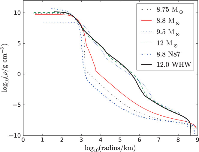
Figure 22. Density profile prior to its collapse for star models of a mass 8.75–12 M⊙. The model is at the moment of Ne-shell ignition (Jones et al. Reference Jones2013). The presupernova density profile of the 8.8 M⊙ model is also presented for contrast (Nomoto et al. Reference Nomoto, Sparks, Fesen, Gull, Miyaji and Sugimoto1982). The solid line is the 12 M⊙ progenitor model presented in Woosley, Heger, & Weaver (Reference Woosley, Heger and Weaver2002).
The low-energy explosion is expected owing to the inherent structure of the ONeMg core during its collapse. Three features in the star support this outcome: (1) there is a small mass mantle; (2) the density gradient is very steep near the core edge; and (3) the H-rich envelope has a very low density. The three factors lead to the occurrence of the explosion in a short time after the core bounce. Without sufficient time for the neutrino driven convection and the standing-accretion shock instability to develop, the explosion is more spherical. This also makes the kick velocity of that neutron star smaller than typical Fe CCSNe.
In Tominaga et al. (Reference Tominaga, Blinnikov and Nomoto2013) and Moriya et al. (Reference Moriya, Tominaga, Langer, Nomoto, Blinnikov and Sorokina2014), the ECSN light curves are calculated from the one-dimensional collapse models. The light curve shape reassembles with a few SNe, suggesting their origin. The classical example is the Crab pulsar evolved from the ancient explosion SN 1054. The higher He abundance, little enhancement of heavy elements (except for Ni), small ejecta mass, and low kinetic energy (Nomoto et al. Reference Nomoto, Sparks, Fesen, Gull, Miyaji and Sugimoto1982; Nomoto Reference Nomoto1985) all favour the explosion originated from the collapse of an ONeMg core. Very recently, Gessner & Janka (Reference Gessner and Janka2018) have shown the existence of the tension between the kick velocity of the Crab pulsar and the hydrodynamical models. This points out the needs for further investigations.
More recent examples include SN 2008S (Prieto et al. Reference Prieto2008; Botticella et al. Reference Botticella2009) and 2008 NGC300-OT (Bond et al. Reference Bond, Bedin, Bonanos, Humphreys, Monard, Prieto and Walter2009). The low luminosity and slow evolution hint on the dust-surrounding bright progenitor, which has a severe mass loss before its final explosion (Kochanek Reference Kochanek2011).
In Figure 22, we show the bolometric light curve from one of the ECSN model. This model assumes a 3.0 M⊙ envelope, with a hydrogen abundance XH = 0.2. The density structure of N87 is assumed as the initial profile. This model is rather different from the collapse progenitor model of mass M = 8.8–12.0 M⊙ we have discussed. By comparing with Figure 22, the density profile, the N87 model shows a more extended envelope but a steeper gradient. In fact, this model has the steepest gradient at core edge among all progenitor models.
In Figure 23 (Tominaga et al. Reference Tominaga, Blinnikov and Nomoto2013), we show the theoretical light curves from ECSNe models evolved from SAGB stars. The optical data from SN 1054 is also presented for comparison. We can see that the bright and short plateau, resulted from the low explosion energy of the ECSN model, is consistent with SN 1054. However, some features are not yet produced. For example, the plateau of light curve, indicated by the luminosity data at about 900 d, hints on a small progenitor envelope mass. Furthermore, the late-time luminosity can provide insight to the power source from the NS. In particular, the spin-down luminosity of the newborn Crab pulsar or circumstellar interaction can be explained by the energy input from the newborn Crab pulsar. This is further supported by the filamentary structures of the Crab Nebula, which demonstrate the circumstellar interaction with the shock front through the Rayleigh–Taylor instabilities.
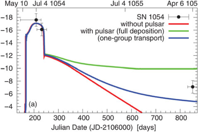
Figure 23. Optical light curves of SN 1054 (black circles) and the ECSNe of the SAGB stars (Tominaga, Blinnikov, & Nomoto Reference Tominaga, Blinnikov and Nomoto2013). The ordinate is the absolute optical magnitude.
The Spitzer (SPIRITS) (Werner et al. Reference Werner2004) have observed recently a new class of obscured, red transients. They have a typical mid-IR luminosities between novae and supernovae that do not exhibit optical counterparts. This class of objects is now called as SPRITEs (eSPecially Red Intermediate-luminosity Transient Events) (Kasliwal et al. Reference Kasliwal2017). Kasliwal et al. (Reference Kasliwal2017) suggest ECSN is one of the possible candidates of SPRITEs. Actually, SAGB stars produce carbon-enhanced circumstellar matter, in which carbon dust can form (see Section 2). Such a dusty circumstellar matter would obscure the progenitor of ECSN. It would be interesting to investigate the interaction of ECSN and the dusty CSM and the observational feature. Furthermore, near IR observations of SPRITEs-like objects with JWST would be interesting.
7.2. Neutrino observables
Besides optical signals, the neutrino-induced explosion is also responsible to produce a transient event in the neutrino, after the formation of the neutron star.
In these collapsing models, the scenario is comparable to that in core-collapse supernovae (CCSN). In this case, the core constantly contracts and reaches a higher central density. The higher density makes more electrons to be captured, which further softens the core. The process continues until the core reaches nuclear density, where the nuclear matter has a much stiffer equation of state. This creates the bounce shock which stops the contraction. Unlike CCSN, there is no massive infalling matter outside the ONeMg core, except for the low-density envelope due to the very sharp core-envelope structure [see e.g., the density profile in Figure 7 in Jones et al. (Reference Jones2013)]. Before the shock reaches the surface, the ONeMg core is still contracting (Phase I). Once the bounce shock reaches the surface of the core, it will excite the surface and eject the outermost layer (Phase II). After that, the neutrino heating can send the matter outside the protoneutron star away in the form of wind (Phase III). In Figure 24, we demonstrate the three phases by showing the radius of the ONeMg core after its collapse has started.
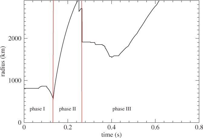
Figure 24. The radius of the ONeMg core after the collapse. Phase I stands for the period before the bounce shock reaches the surface. Phase II stands for the period where the first shock excites the outermost material and ejects it away. Phase III stands for the period where the protoneutron star has settled down and the neutrino emission can gradually eject the outermost matter in the form of wind.
The collapse of electron capture supernova and low-mass iron core are not well studied until the last decades, partly motivated by the sophistication of neutrino transport in multi-dimensional simulations [e.g., Müller, Janka, & Dimmelmeier (Reference Müller, Janka and Dimmelmeier2010), Müller, Janka, & Marek (Reference Müller, Janka and Marek2012), Müller, Janka, & Marek (Reference Müller, Janka and Marek2013), and Müller & Janka (Reference Müller and Janka2014)] and the existence of the progenitor models from a consistent stellar evolution model (Jones et al. Reference Jones2013; Doherty et al. Reference Doherty, Gil-Pons, Siess, Lattanzio and Lau2015; Woosley & Heger Reference Woosley and Heger2015). One-dimensional [e.g., (Hüdepohl et al. Reference Hüdepohl, Müller, Janka, Marek and Raffelt2010) and Radice et al. (Reference Radice, Burrows, Vartanyan, Skinner and Dolence2017)] and multi-dimensional simulations [e.g., Wongwathanarat et al. (Reference Wongwathanarat, Janka and Müller2013), Radice et al. (Reference Radice, Burrows, Vartanyan, Skinner and Dolence2017), Melson, Janka, & Marek (Reference Melson, Janka and Marek2015), Wanajo et al. (Reference Wanajo, Müller, Janka and Heger2018), and Gessner & Janka (Reference Gessner and Janka2018)] are progressively made for extracting the interaction of neutrino heating/cooling on the formation of large-scale asymmetry and the following explosion. Unlike the core-collapse supernova counterpart, the typical asymmetry for ONeMg core is much smaller. Some further studies concerning on the neutrino physics, such as the neutrino flavor oscillations, can be found in the literature (Pllumbi et al. Reference Pllumbi, Tamborra, Wanajo, Janka and Hüdepohl2015).
7.2.1. Numerical methods
Here, we briefly introduce how ECSN explosion looks like. To do the estimation, we have relied on the one-dimensional hydrodynamics, with the neutrino transport called the advanced leakage scheme (ALS) from Perego, Cabezon, & Käppeli (Reference Perego, Cabezon and Käppeli2016). The scheme provides a quick diagnosis to the neutrino signature based on an improved version of predecessor, namely the leakage scheme (Rosswog & Liebendörfer Reference Rosswog and Liebendörfer2003), with improvement based on the isotropic diffusion source approximation (IDSA) (Liebendörfer, Whitehouse, & Fischer Reference Liebendörfer, Whitehouse and Fischer2009). We present the important equations which we have used in this modelling, and we refer the readers to the original instrument paper for the detailed derivation and the spirit of these approximations.
In this scheme, the neutrinos are not only emitted by matter as in the leakage scheme but also can be transported and absorbed as in IDSA. The major approximation for the neutrino-transparent zones is that, it evolves to asymptotically to the solution of the diffusive regime. This greatly simplifies the root-finding section by iteration as common in neutrino solver including IDSA, where in scenarios of strong shocks, it is possible for the root-finder to fail in finding the new thermodynamics states for a given density and temperature, especially when there are temperature floor and ceiling owing to the finite size EOS table. Also, in multi-dimensional Eulerian hydrodynamics simulations, the advection term always bring noises to the system. The residue error can lead to instability of the root-finding subroutines.
The essence of this scheme is that one uses the averaged quantities Yv ,i and Zv ,i which represent the mean neutrino number fraction and mean neutrino particle energy for the ith-type neutrino  $(i = e, \bar{e})$. By doing that, one can bypass the needs of calculating all energy bands for each flavor of neutrino and focus on the overall interaction. That says
 \begin{eqnarray}Y_{\nu,{\rm i}} = \frac{4 \pi}{(h c)^3} \frac{m_B}{\rho} \int f^{{\rm tr}}_{\nu,i} E^2 {\rm d}E,\end{eqnarray}
 \begin{eqnarray}Z_{\nu,{\rm i}} = \frac{4 \pi}{(h c)^3} \frac{m_B}{\rho} \int f^{{\rm tr}}_{\nu,i} E^3 {\rm d}E.\end{eqnarray} $f^{{\rm tr}}_{\nu,i}$ is the occupation number of the ith-type neutrino, mB is the nucleon mass. These variables satisfy the transport equations
 \begin{eqnarray}\frac{\partial Y_{\nu,{\rm i}}}{\partial t} + \textbf{\textit{v}} \cdot Y_{{\rm \nu,i}} = \dot{Y}_{{\rm \nu,i}},\end{eqnarray}
 \begin{eqnarray}\frac{\partial Z_{\nu,{\rm i}}^{3/4}}{\partial t} + \textbf{\textit{v}} \cdot Z_{{\rm \nu,i}}^{3/4} = \frac{3}{4} \rho^{3/4} \dot{Z}_{{\rm \nu,i}}.\end{eqnarray}
The ALS is more improved from the former version by including the extra degree of freedom that Yv and Zv are another two hydrodynamics scalar variables which follows the fluid motion. Therefore, the local neutrino properties inside the neutrino photosphere can be made to change according to the matter properties.
The ALS assumes that the neutrinos can transport in two ways: in the optically deep zones, neutrino can diffuse from the core outwards and they leak out around the neutrino photosphere. They are in equilibrium with the nucleons by the beta-equilibrium and they can be scattered by nucleons, i.e.,
 \begin{eqnarray}\nu_e + n \rightarrow p + e^-,\end{eqnarray}
 \begin{eqnarray}\nu_{\bar{e}} + p \rightarrow n + e^+,\end{eqnarray}
and the elastic scattering processes
 \begin{equation} N + \nu_i \rightarrow N + \nu_i, \end{equation}
with N being the nucleon (proton or neutron) and vi being all types of neutrinos. In this work, we only model electron neutrino ve and anti-electron neutrino  $\nu_{\bar{e}}$. The interaction between neutrino and nuclei is neglected because the important part of the neutrino transport goes to the core, while they are free from nuclei in the density and temperature range we are considering. In the optically transparent zones, the neutrino can freely propagate but can still deposit energy to the baryonic matter.
So, the coupling term between the neutrino species and the baryonic matter is characterised by the change of local lepton number  $\dot{Y}_l$ and the local net energy change $\dot{u}_{\nu}$:
 \begin{eqnarray}\dot{Y}_1 = \dot{Y}_e + \dot{Y}_{\nu_{e}} - \dot{Y}_{\bar{\nu}_{e}},\end{eqnarray}
 \begin{eqnarray}\dot{u}_{\nu} = \dot{q}_{\nu} + \frac{1}{m_B} \big(\dot{Y}_e + \dot{Y}_{\nu_{e}} - \dot{Y}_{\bar{\nu}_{e}}\big).\end{eqnarray}
The terms on the left-hand side are the net gain/loss of neutrino and specific internal energy for a given mesh, while  $\dot{Y}_e$ and $\dot{q}_{\nu}$ are those for the matter. The remaining terms are those for the neutrinos. The two equations govern the conservation of lepton and energy during its interaction with electrons and nucleon. Terms on the right-hand side stand for the local changes of electron fraction ( $\dot{Y}_e$) and electron and anti-electron neutrino fractions ( $\dot{Y_{\nu_{e}}}$ and $\dot{Y}_{\bar{\nu}_{e}}$).
One major simplification in ALS is that it uses the notation of timescale to avoid calculating the diffusion of neutrino directly, which involves solving an elliptic equation for the diffusion process. The timescale is defined and then we calculate the change of the neutrino energy distribution by considering the processes of neutrino production and diffusion.
 \begin{equation}
\frac{{\rm d}f^{{\rm tr}}_{\nu}}{{\rm d}t} = \dot{f}^{\kern0.7pt \rm tr}_{\nu,{\rm prod}} + \dot{f}^{\kern0.7pt \rm tr}_{\nu,{\rm diff}}.
\end{equation}
\begin{equation}
\frac{{\rm d}f^{{\rm tr}}_{\nu}}{{\rm d}t} = \dot{f}^{\kern0.7pt \rm tr}_{\nu,{\rm prod}} + \dot{f}^{\kern0.7pt \rm tr}_{\nu,{\rm diff}}.
\end{equation}
Assuming both terms always leads to some equilibrium states, we have
 \begin{equation}
\dot{f}^{\rm tr}_{\nu,{\rm prod}} = \frac{((f_{\nu})_{{\rm eq}} - f^{{\rm tr}}_{\nu}}{\max (t_{\nu,{\rm prod}}, \Delta t)}\exp \left( - \frac{t_{\nu,{\rm prod}}}{t_{\nu,{\rm diff}}} \right)
\end{equation}
\begin{equation}
\dot{f}^{\rm tr}_{\nu,{\rm prod}} = \frac{((f_{\nu})_{{\rm eq}} - f^{{\rm tr}}_{\nu}}{\max (t_{\nu,{\rm prod}}, \Delta t)}\exp \left( - \frac{t_{\nu,{\rm prod}}}{t_{\nu,{\rm diff}}} \right)
\end{equation}
and
 \begin{equation}
\dot{f}^{\rm tr}_{\nu,{\rm diff}} = -\frac{f^{{\rm tr}}_{\nu}}{\max (t_{\nu,{\rm diff}}, \Delta t)}\exp \left( - \frac{t_{\nu,{\rm diff}}}{t_{\nu,{\rm prod}}} \right)
\end{equation}
\begin{equation}
\dot{f}^{\rm tr}_{\nu,{\rm diff}} = -\frac{f^{{\rm tr}}_{\nu}}{\max (t_{\nu,{\rm diff}}, \Delta t)}\exp \left( - \frac{t_{\nu,{\rm diff}}}{t_{\nu,{\rm prod}}} \right)
\end{equation}
These two expressions make sure when production dominates the neutrino process, namely when tv ,prod ≪ tv ,diff, the neutrino spectra evolve to the new equilibrium; while when diffusion dominates the process, neutrino decays exponentially. The corresponding timescales are given in the following
 \begin{equation}
t_{\nu, {\rm prod}}(E,r) = \frac{1}{j_{\nu} (E,r)},
\end{equation}
\begin{equation}
t_{\nu, {\rm prod}}(E,r) = \frac{1}{j_{\nu} (E,r)},
\end{equation}
and
 \begin{equation}t_{\nu, {\rm diff}}(E,r) = \frac{\Delta x_{\nu}}{c} \tau_{\nu, {\rm tot}}(E,r),\end{equation}
where
 \begin{equation}\Delta x_{\nu} = \alpha_{{\rm diff}} \tau_{\nu, {\rm tot}}(E,r) \lambda_{\nu, {\rm tot}}(E,r)\end{equation}
is the effective length scale of diffusion. Having known the rate of change of  $f_{{\rm tr}_{\nu}}$, the new tapped component neutrino energy spectra can be calculated and $f^{{\rm tr}}_{\nu, t+ \Delta t}$ can be obtained. This provides new Yv and Zv accordingly.
7.2.2. Collapse dynamics
In Figure 25, we plot the neutrino signal of one of the ONeMg models which collapses. To compare with, we also plot that from the collapse of a cold WD as an AIC. It can be seen that the typical collapse process, as seen from the neutrino, is very similar to the AIC.

Figure 25. The neutrino signals from a cold collapse of a white dwarf and from the deflagration-collapse of an ONeMg core. The gravitational collapse of an AIC is also shown for comparison.
We choose to show the AIC because the scneario for the collapse of an ECSN is very similar in the collapse progenitor. In both cases, it is an individual white dwarf that collapses by its gravitational instability. Also, both channels are the current candidates for explaining the origin of low-mass neutron stars (Schwab et al. Reference Schwab, Podsiadlowski and Rappaport2010) (with a mass 1–1.2 M⊙). For AIC, the binary star channel is necessary since it involves the sub-Chandrasekhar mass white dwarf to accrete matter from its companion star in the red giant phase, so that there can be mass transfer by Roche-lobe overflow. In Nomoto (Reference Nomoto1982) and Nomoto & Kondo (Reference Nomoto and Kondo1991), in order for the white dwarf to collapse instead of having a nova event or direct explosion as a Type Ia(x) supernova, the accretion rate should be above 10−8M⊙ yr−1 for ONeMg white dwarf and 10−6M⊙ yr−1 for CO white dwarf.
Before bounce, the neutrino signal gradually increases due to the growing electron capture in the core, including the capture by nuclei and by proton. At the moment of bounce, the electron neutrino bursts out. It quickly reduces to a constant value within 0.1 s. On the other hand, there is no anti-electron neutrino at the beginning since it requires reactions with positron, which exists in a very small amount due to the high Fermi energy. Following the neutronisation, the electron number drops. The first peak of anti-neutrino appears about 0.15 s after bounce. This is because most anti-neutrino is created thermally, where thermalised matter appear only after the bounce shock has passed through. In this calculation, only the essential reactions are included [see Equation (71)]. The source term of the positron comes only from the positron capture similar to the electron capture. This also explains a slightly lower anti-electron neutrino in the neutrino luminosity after bounce.
In Figure 26, the velocity profiles at different time are plotted for the same model. At the beginning, the infall velocity is too low to be seen. At bounce, a rapid inflow has formed to about 100 km, with a maximum velocity of 0.08c. The velocity decreases with radius. This shows that the stiff nuclear matter is very efficient to the accretion of matter on to the NS envelope. Later, when the shock approaches the surface, it creates a clear signature to the compression between the ingoing matter and the outgoing shock. At the same time, the constant ejection of neutrino from the NS has become an important source of energy. As seen in the outer part of the star, the star is creating neutrino-induced wind. The wind can reach as high as 0.07c, which is higher than the escape velocity. On the other hand, the thermalised core has almost no motion. Within the first 100 km, there is almost no motion of the NS, showing that this layer of material is less affected by the neutrino-induced wind.
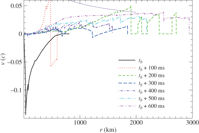
Figure 26. The velocity profiles at different time after the collapse of an ONeMg model.
7.3. Chemical observables
The explosion of the super-AGB star is not well considered in the literature, because its collapse into a neutron star means most of the heavy elements are trapped in the neutron star. A small amount of ejecta (∼10−2) is observed. Certainly, prior to the collapse, during the AGB phase, the mass loss through wind can eject significant amount of heavy elements, such as s-process elements, produced during the hot bottom burning and dredge-up (Busso et al. Reference Busso, Gallino and Wasserburg1999, Doherty Reference Doherty, Gil-Pons, Lau, Lattanzio and Siess2014a, Doherty et al. Reference Doherty, Gil-Pons, Lau, Lattanzio, Siess and Campbell2014b).
Despite that, recent one-dimensional and multi-dimensional hydrodynamics simulations of ECSN have shown that the ejecta contains neutron-rich isotopes which can explain the origin of isotopes like 48Ca (Wanajo, Janka, & Müller Reference Wanajo, Janka and Müller2013a) and 60Fe (Wanajo, Janka, & Müller Reference Wanajo, Janka and Müller2013b). Unlike the one-dimensional model, the multi-dimensional model allows mixing of low Ye matter near the protoneutron star to the surface. These matter can have an Ye as low as 0.40 (Wanajo, Janka, & Müller Reference Wanajo, Janka and Müller2011). Such mixing allows the ejecta to contain those neutron-rich isotopes such as 48Ca, 50Ti, 54Cr, and 60Fe. In (Wanajo et al. Reference Wanajo, Müller, Janka and Heger2018), it is further confirmed that ECSN can be one of the major origins of light trans-Fe elements including Zn, Ge, As, Se, Br, Kr, Rb, Sr, Y, and Zr in the Galaxy. The role of ECSN is studied in the galactic chemical evolution (Takahashi et al. Reference Takahashi, Yoshida and Umeda2013). The rich production of trans-Fe elements, such as Zn, is shown to be able to explain the Zn abundance in the dwarf spheroidal galaxies.
8. Conclusion
In this review, we discuss the progenitor evolution and some of the modelling technique related to ECSNe in ONeMg core. The ECSN is an important candidate of object responsible for producing the lower-mass branch of neutron stars. In this review, we summarise the input physics and the critical components that influence the final evolution of the ONeMg core. The hydrodynamics, nuclear reactions, weak interactions, sub-grid turbulence, and turbulent flame prescription are discussed. The physical components such as the central density, properties of the initial flame, and the input physics are discussed. The extension from ONeMg cores to CO white dwarfs is considered. Similar explosion–collapse bifurcation for the models of similar configurations is observed. At last, the possible observational hints of this class of objects is discussed.
From this review, it becomes clear that for a typical ONeMg core which is likely to trigger the ONe deflagration at a central density of 109.95 g cm−3, the core is likely to collapse for a wide range of parameters, including different flame structure and flame size. Thus, it is very likely the low-mass neutron star originates as an final product of 8–10 M⊙ stars. However, the sensitivity of the final core evolution an accurate understanding to the evolution of SAGB stars is important. The uncertainties, coming from both numerical modelling in stellar evolution, and the simplified recipes in the multi-dimensional simulations, show that a more comprehensive study of SAGB star and its related study of ECSNe remain important.
Author ORCIDs
Shing-Chi Leung, https://orcid.org/0000-0002-4972-3803; Ken’ichi Nomoto, https://orcid.org/0000-0001-9553-0685
Acknowledgements
This work has been supported by the World Premier International Research Center Initiative (WPI Initiative), MEXT, Japan, and JSPS KAKENHI Grant Nos. JP26400222, JP16H02168, and JP17K05382, and the Endowed Research Unit ‘Dark side of the Universe’ by Hamamatsu Photonics K.K. at Kavli IPMU.


