


1. Introduction
The scope of this investigation is to verify if linear stability analysis can be used to explain and predict the onset of large-scale convection rolls in unstably stratified turbulent shear flows. The motivation of the study is twofold. First, there is a continuing and growing interest in the dynamics of large-scale coherent structures in turbulent shear flows that contain most of the turbulent kinetic energy at high Reynolds numbers and provide the energy injection mechanism in most turbulent flows. Despite the general consensus that large-scale instabilities and/or non-modal energy amplification mechanisms explain the existence of these coherent structures, and the many linear analyses of turbulent mean flows, only a few studies provide quantitative comparisons of theory and observations, in particular in what concerns the critical parameter values for the instability onset. There is, therefore, a need to test linear stability analyses on a well-defined turbulent shear flow where the onset of a large-scale instability is well defined and the comparison of the predicted critical values with (numerical) experiments is possible.
The second motivation stems from the recent resurgence of dichotomies in the definition of the linear operator used for the linear analysis of turbulent mean flows, where in some studies the effect of turbulent Reynolds stresses is embedded in the linear operator, while it is not in other studies. Furthermore, in some analyses, the perturbation to the turbulent mean flow is considered in a statistical sense i.e. considering perturbations that are averaged fields, while in other analyses, perturbations are non-averaged quantities. These differences lead to ambiguities in the interpretation of theoretical predictions and in their comparison to observations as well as in nonlinear theories that would be built on top of the linear analyses, probably hindering further substantial progress in the field.
A brief discussion of these two sets of motivations is provided below.
1.1. Onset of coherent convection rolls
In many situations, ranging from atmospheric boundary layers to heat exchangers, a wall-bounded mean flow, generally driven by a pressure gradient, is affected by buoyancy effects, generally associated with heating and cooling from the boundaries. In the case where the bottom fluid layers are denser than the top layers, buoyancy effects are stabilizing. In the opposite situation, where e.g. the fluid is heated from below, buoyancy effects are destabilizing, inducing transition to turbulence if the flow is laminar or increasing turbulent fluctuations if it is already turbulent (see e.g. Turner Reference Turner1979). In this case, the flow structure depends strongly on the relative importance of buoyancy and shear-induced kinetic energy production as well as momentum and thermal diffusion. The two most studied situations are the two extreme cases of natural convection in the absence of mean flow (see e.g. Chandrasekhar Reference Chandrasekhar1961; Bodenschatz, Pesch & Ahlers Reference Bodenschatz, Pesch and Ahlers2000; Ahlers, Grossmann & Lohse Reference Ahlers, Grossmann and Lohse2009) and of forced convection, where mean advection is dominant and temperature fluctuations behave as passive scalars (see e.g. Schlichting Reference Schlichting1979; Turner Reference Turner1979). In between these two extreme cases is the mixed-convection regime, which is often characterized by large-scale coherent structures that influence strongly the vertical momentum and heat transport.
Probably the most impressive large-scale coherent structures observed in the mixed-convection regime are the rolls observed frequently in unstably stratified atmospheric boundary layers, which have been associated to cloud streets extending up to several hundred kilometres and persisting up to several days (see the reviews of Kuettner Reference Kuettner1959; Brown Reference Brown1980; Etling & Brown Reference Etling and Brown1993; Atkinson & Wu Zhang Reference Atkinson and Wu Zhang1996). Numerous studies have investigated the origin of these rolls, suggesting that both inflectional and convective instabilities play a role in their amplification (see, among many others, LeMone Reference LeMone1973; Brown Reference Brown1980; Etling & Brown Reference Etling and Brown1993). Despite the many studies, however, the comparison of theoretical predictions and field measurement remains difficult because of the large gap between the simplifying assumptions and idealized mean flows used in theoretical analyses and the reality characterized by extremely large Reynolds numbers, heterogeneous and unsteady mean flows, and complicated ground topography. An example of this unsettled state of affairs is the recent conclusion of Jayaraman & Brasseur (Reference Jayaraman and Brasseur2021), who, referring to the onset of large-scale elongated structures in their large-eddy simulations of the atmospheric boundary layer, state: ‘The mechanisms that underlie the restructuring of the ABL at the very low levels of surface heat flux in the critical state … are unknown’.
An additional difficulty, discussed e.g. by Brown (Reference Brown1980), is that large-scale rolls observed in the field are often far from the onset of the instability and, being in the finite-amplitude (nonlinearly saturated) regime, their comparison with linear stability predictions is questionable.
It is therefore important that linear theory predictions are compared to experimental or numerical data in settings that (a) can be driven close to the onset of the linear instability, where critical parameters values can be determined, and (b) are well controlled and substantially match the assumptions of the theoretical analyses. This is precisely the aim of the present study.
1.2. Definition of the linear operator for stability analyses
The stability analysis of turbulent wall-bounded flows has a long history going back at least to the seminal works of Malkus (Reference Malkus1956), Reynolds & Tiederman (Reference Reynolds and Tiederman1967) and Reynolds & Hussain (Reference Reynolds and Hussain1972). In these early studies, the linear stability of the turbulent mean flow is analysed with the method of normal modes. However, while Malkus (Reference Malkus1956) does not include the effect of turbulent Reynolds stresses in the stability analysis embedded in his theory, Reynolds & Tiederman (Reference Reynolds and Tiederman1967) and Reynolds & Hussain (Reference Reynolds and Hussain1972) do include their effect by modelling them by means of an eddy viscosity. Since then, these two different approaches have persisted in the linear analysis of turbulent mean flows. In the first approach the linear dynamics of instantaneous (deterministic, non-averaged) turbulent fluctuations  $\boldsymbol {u}'$ to the temporally averaged turbulent mean flow $\boldsymbol {U}$ is considered, and the Navier–Stokes operator is linearized near the turbulent mean flow, while nonlinear terms and Reynolds stresses are either neglected or included/modelled in a forcing term that provides input to the linear operator (see, among others, Malkus Reference Malkus1956; Butler & Farrell Reference Butler and Farrell1993; Farrell & Ioannou Reference Farrell and Ioannou1993; McKeon & Sharma Reference McKeon and Sharma2010; McKeon Reference McKeon2017). This approach will be referred to as ‘quasi-laminar’ because the linear operator is formally identical to the one used to analyse the stability of laminar flows, except for the use of turbulent mean profiles as basic flows.
In the second approach, a distinction is made between (generally unsteady and spatially inhomogeneous) coherent perturbations  $\widetilde {\boldsymbol {u}}$ to the temporally-averaged turbulent mean flow $\boldsymbol {U}$ and the residual (random, incoherent) perturbations $\boldsymbol {u}"$, where $\widetilde {\boldsymbol {u}}$ is such that $\langle \boldsymbol {u} \rangle =\boldsymbol {U} + \widetilde {\boldsymbol {u}}$, and $\boldsymbol {u}''$ satisfies $\langle \boldsymbol {u}'' \rangle = \boldsymbol {0}$, with the averaging operator $\langle\,\cdot\,\rangle$ representing e.g. the ensemble average or the phase average or spatial filtering. We refer the reader to Reynolds & Hussain (Reference Reynolds and Hussain1972) for more details on this triple decomposition.
The linear dynamics of the coherent perturbations  $\widetilde {\boldsymbol {u}}$ is then analysed by including the effect of Reynolds stresses in the linear operator (see, among others, Reynolds & Hussain Reference Reynolds and Hussain1972; Etling & Wippermann Reference Etling and Wippermann1975; Bottaro, Souied & Galletti Reference Bottaro, Souied and Galletti2006; del Álamo & Jiménez Reference del Álamo and Jiménez2006; Cossu, Pujals & Depardon Reference Cossu, Pujals and Depardon2009; Crouch et al. Reference Crouch, Garbaruk, Magidov and Travin2009; Pujals et al. Reference Pujals, García-Villalba, Cossu and Depardon2009; Hwang & Cossu Reference Hwang and Cossu2010a,Reference Hwang and Cossub; Willis, Hwang & Cossu Reference Willis, Hwang and Cossu2010; Tammisola & Juniper Reference Tammisola and Juniper2016; Illingworth, Monty & Marusic Reference Illingworth, Monty and Marusic2018; Morra et al. Reference Morra, Semeraro, Henningson and Cossu2019; Pickering et al. Reference Pickering, Rigas, Schmidt, Sipp and Colonius2021; Madhusudanan et al. Reference Madhusudanan, Illingworth, Marusic and Chung2022). This approach will be referred to as ‘statistical-linear’ because the linear dynamics of averaged perturbations is considered and the linear operator differs from the laminar one because of additional terms modelling the averaged effect of residual random motions on the coherent ones.
A resurgence in the dichotomy of linear operator definitions is linked to the recent interest in situations where the turbulent mean profile is linearly stable and the (forced) response is expressed conveniently by means of the resolvent operator. As forcing inputs, which include nonlinear terms, are generally unknown, resolvent analyses have modelled them mostly as (delta-correlated) white noise. However, it has been shown recently that while this specific noise assumption leads to realistic predictions for second-order velocity cross-spectral densities when the resolvent operator includes the modelling of Reynolds stresses (statistical-linear approach), this is not the case when the quasi-linear resolvent is used (Morra et al. Reference Morra, Semeraro, Henningson and Cossu2019). Two different main roads have therefore been taken to make further progress: the first pushes the statistical-linear formulation into the nonlinear domain by making use of more advanced Reynolds stress models such as those implemented in large-eddy simulations (see e.g. Hwang & Cossu Reference Hwang and Cossu2010c, Reference Hwang and Cossu2011; Rawat et al. Reference Rawat, Cossu, Hwang and Rincon2015; Cossu & Hwang Reference Cossu and Hwang2017), while the second looks for models for the forcing correlations (see e.g. Nogueira et al. Reference Nogueira, Morra, Martini, Cavalieri and Henningson2021). In the case of linearly stable mean flows, it is therefore unlikely that a consensus on the best linear operator to be used for the analysis of turbulent mean flows will emerge soon because the ambiguity on the best way to account for Reynolds stresses (in the linear operator or in the forcing terms?) is likely to persist. However, this ambiguity can be removed by considering the onset of linear modal instabilities where the linear response is dominated by the unstable normal mode and not by the response to forcing. The second motivation of the present study is therefore to examine the intrinsic properties of linear operators to be used in linear analyses of turbulent mean flows without the complications related to the modelling of the forcing terms. This will be achieved by determining the critical Rayleigh (or Richardson) number where coherent large-scale rolls become unstable in a high-Reynolds-number turbulent channel flow.
1.3. Outline
We will consider the pressure-driven turbulent Poiseuille flow between two parallel isothermal smooth walls to which a destabilizing temperature difference is applied. In this setting, most of the complications associated with the much-studied atmospheric boundary layer case – such as the effects of ground roughness, mean flow unsteadiness, capping inversions, system rotation, three-dimensional mean flow profiles and associated inflection points – are removed. Furthermore, in this setting, theoretical predictions of the critical Richardson and/or Rayleigh numbers, as well as their dependence on the Reynolds number, can be tested against the recent direct numerical simulations (DNS) of Pirozzoli et al. (Reference Pirozzoli, Bernardini, Verzicco and Orlandi2017).
We will therefore proceed by considering the effect of increasing Richardson numbers (or equivalently Rayleigh numbers) on the turbulent channel flow operated at constant Reynolds number and fixed Prandtl number (all results are obtained for  $Pr=1$). The simulations of Pirozzoli et al. (Reference Pirozzoli, Bernardini, Verzicco and Orlandi2017) show that, as expected, in the forced convection regime, before the onset of large-scale rolls, the temperature field behaves as a passive scalar, leaving the mean velocity and temperature profiles essentially unchanged (when properly normalized). These forced convection mean velocity and temperature profiles are used as basic flows for the linear stability analysis.
This approach is different from the one followed by Madhusudanan et al. (Reference Madhusudanan, Illingworth, Marusic and Chung2022), who, in a study published during the revision of this paper, investigate the impulse response of the linear system based on the statistical-linear approach but linearized about the turbulent mean flows of Pirozzoli et al. (Reference Pirozzoli, Bernardini, Verzicco and Orlandi2017) computed by DNS also in the mixed-convection regime in the presence of finite-amplitude large-scale convective structures. Doing so, Madhusudanan et al. (Reference Madhusudanan, Illingworth, Marusic and Chung2022) are able to show that some features of the large-scale convection are reproduced by the linear impulse response, but they do not compute the critical Richardson/Rayleigh numbers or the critical modes corresponding to the onset of large-scale convection.
The paper is organized as follows. The mathematical formulation of the problem, and in particular of the linear stability analysis, is introduced in § 2. The critical Richardson and Rayleigh numbers, as well as the critical wavenumbers and the critical mode, are then computed in § 3 for a particular Reynolds number for which DNS data are available and well converged. The dependence of the critical values on the Reynolds number is addressed in § 4 by making use of basic flows based on a semi-empirical model described in Appendix A, which extends the one proposed by Cess (Reference Cess1958) to the non-isothermal case. A summary of the results and a discussion of their main implications are provided in § 5.
2. Mathematical model
We consider the pressure-driven flow of a viscous fluid of kinematic viscosity  $\nu$, thermal diffusivity $\alpha$, and thermal expansion coefficient $\beta$, in the channel between two infinite parallel walls normal to the gravitational field $-g\boldsymbol {e}_z$ and located at $z^*=\pm h$, where $z^*$ is the (dimensional) vertical coordinate and $\boldsymbol {e}_z$ is the unit vector oriented along the $z$ axis. We denote by $x$,
$x$,  $y$ and $z$ the streamwise, spanwise and vertical coordinates, respectively, made dimensionless with respect to the channel half-height $h$. The distance from the walls, scaled in wall (inner) units, is $z^+=(h - |z^*|) u_\tau / \nu$, where $u_\tau =\sqrt {\tau /\rho }$ is the characteristic velocity associated with the wall shear stress $\tau$. A temperature difference $\Delta \varTheta$ is maintained between the two walls, which are assumed to be isothermal, resulting in a vertical heat flux $Q$. In the following, we will deal with the case where the flow is turbulent and the bottom wall is hotter than the top wall, and for simplicity, define $Q \geq 0$, $\Delta \varTheta \geq 0$ in this situation.
We are interested in the onset of large-scale turbulent convection in already turbulent wall-bounded shear flows as the temperature difference and the heat flux are increased gradually, starting from zero. For this purpose, we use a ‘statistical-linear’ approach built on the linear model proposed by Reynolds & Hussain (Reference Reynolds and Hussain1972) and used by del Álamo & Jiménez (Reference del Álamo and Jiménez2006), Pujals et al. (Reference Pujals, García-Villalba, Cossu and Depardon2009), Hwang & Cossu (Reference Hwang and Cossu2010a,Reference Hwang and Cossub) and others to describe the dynamics of small-amplitude coherent perturbations  $\boldsymbol {u}=(u,v,w)$, $p$ and $\theta$ (velocity, pressure and temperature, where the usual $\ \widetilde {\,}\ $ is dropped for simplicity) to the temporally averaged mean flow $\boldsymbol {U}=U(z)\,\boldsymbol {e}_x$, $P(z)$ and $\varTheta (z)$, by including the effect of heat transport under the Boussinesq approximation. To improve the convergence of the temporal averaging, it is usual to compute $U(z)$, $P(z)$ and $\varTheta (z)$ by averaging also in the horizontal planes. When expressed in dimensionless units based on the channel half-height $h$, the wall-temperatures difference $\Delta \varTheta$ and the friction velocity ${u_\tau }$, the linear model reads
 \begin{gather} \partial_t \boldsymbol{u} ={-} \boldsymbol{\nabla} \boldsymbol{u} \boldsymbol{\cdot} \boldsymbol{U}-\boldsymbol{\nabla} \boldsymbol{U} \boldsymbol{\cdot} \boldsymbol{u} - Ri_\tau\,\theta \boldsymbol{e}_z -\boldsymbol{\nabla} p + \boldsymbol{\nabla} \boldsymbol{\cdot} \left[ \nu_T \left(\boldsymbol{\nabla} \boldsymbol{u} +\boldsymbol{\nabla} \boldsymbol{u}^{\rm T} \right) \right], \end{gather}
 \begin{gather}\partial_t \theta ={-} \boldsymbol{\nabla} \theta \boldsymbol{\cdot} \boldsymbol{U}-\boldsymbol{\nabla} \varTheta \boldsymbol{\cdot} \boldsymbol{u} +\boldsymbol{\nabla} \boldsymbol{\cdot} \left(\alpha_T\,\boldsymbol{\nabla} \theta \right), \end{gather}
where, for simplicity, we assume  $Ri_\tau > 0$ in the unstably stratified case. The $\boldsymbol {u}(x,y,z,t)$, $p(x,y,z,t)$ and $\theta (x,y,z,t)$ fields represent coherent motions that are the difference between the (ensemble-averaged or phase-averaged or locally-filtered, etc.) mean fields and the temporally averaged fields $\boldsymbol {U}(z)$, $P(z)$ and $\varTheta (z)$. These coherent motions feel the effect of the residual (random, ‘incoherent’) turbulent fluctuations through Reynolds stresses modelled via eddy viscosity $\nu _t$ and eddy diffusivity $\alpha _t$, which are included in the total eddy viscosity $\nu _T=(1+\nu _t/\nu )/Re_\tau$ and diffusivity $\alpha _T=(1+\alpha _t/\alpha )/(Re_\tau \,Pr)$ expressed in dimensionless form. The system depends on the Prandtl number $Pr=\nu /\alpha$, the friction Reynolds number $Re_\tau =h {u_\tau } /\nu$ and the friction Richardson number $Ri_\tau =h \beta g\,\Delta \varTheta / {u_\tau }^2$. For the sake of comparison with previous investigations, however, results will be presented mainly in terms of the Reynolds and Richardson numbers $Re_b=2 h u_b / \nu$, $Ri_b=2 h \beta g\,\Delta \varTheta / u_b^2$ – based on the bulk velocity $u_b$ – and the Rayleigh and Nusselt numbers $Ra=8 h^3 g \beta \,\Delta \varTheta / (\alpha \nu )$, $Nu=2 h Q / (\alpha \,\Delta \varTheta )$, where the relations $Ra=Ri_b\,Pr\, Re_b^2 = 8\,Ri_\tau \,Pr\, Re_\tau ^2$ hold.
Equations (2.1) and (2.2) can be reduced by standard manipulations (see e.g. Pujals et al. Reference Pujals, García-Villalba, Cossu and Depardon2009; Hwang & Cossu Reference Hwang and Cossu2010a; Jerome, Chomaz & Huerre Reference Jerome, Chomaz and Huerre2012; Madhusudanan et al. Reference Madhusudanan, Illingworth, Marusic and Chung2022) to the following extended Orr–Sommerfeld–Squire system for the wall-normal velocity, wall-normal vorticity and temperature Fourier modes  ${\hat {w}}$, ${\hat {\zeta }}$, ${\hat {\theta }}$ of streamwise and spanwise wavenumbers $k_x$ and $k_y$:
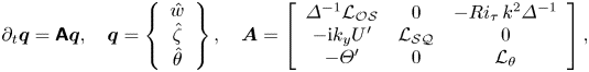 \begin{equation} \partial_t \boldsymbol{q} = \boldsymbol{\mathsf{A}} \boldsymbol{q},\quad \boldsymbol{q}=\left\{\begin{array}{c} \hat{w} \\ \hat{\zeta} \\ \hat{\theta} \end{array}\right\},\quad \boldsymbol{A}=\left[\begin{array}{ccc} \varDelta^{{-}1}\mathcal{L_{OS}} & 0 & -Ri_\tau\,k^2 \varDelta^{{-}1} \\ -{\rm i}k_y U' & \mathcal{L_{SQ}} & 0 \\ -\varTheta' & 0 & \mathcal{L_{\theta}} \end{array}\right], \end{equation}
where  $\boldsymbol {q}$ is the state vector, and $\boldsymbol {A}$ includes the Orr–Sommerfeld–Squire and thermal linear operators generalized to include the effects of eddy viscosity and eddy thermal diffusivity:
 \begin{gather} \mathcal{L_{OS}}={-}{\rm i}k_x(U \varDelta-U'') +\nu_T \varDelta^2+2 \nu_T' \varDelta \mathcal{D} +\nu_T''(\mathcal{D}^2+k^2), \end{gather}
 \begin{gather}\mathcal{L_{SQ}}={-}{\rm i}k_x U + \nu_T \varDelta+\nu_T' \mathcal{D},\quad \mathcal{L_{\theta}}={-}{\rm i}k_x U + \alpha_T \varDelta+\alpha_T' \mathcal{D}, \end{gather}
with  $\mathcal {D}$ and $'$ denoting ${\rm d}/{\rm d}z$, $k^2=k_x^2+k_y^2$ and $\varDelta =\mathcal {D}^2-k^2$. Homogeneous boundary conditions, corresponding to no-slip and isothermal boundary conditions, are enforced on both walls: $\hat {w}(\pm 1)=0$, $\mathcal {D}\hat {w}(\pm 1)=0$, $\hat {\zeta }(\pm 1)=0$, $\hat {\theta }(\pm 1)=0$.
The linear operators in (2.3a–c), (2.4) and (2.5a,b) depend on the temporally averaged mean profiles  $U(z)$, $\varTheta (z)$, and eddy viscosity and diffusivity profiles $\nu _t(z)/\nu$, $\alpha _t(z)/\alpha$. In the following, these profiles will be based either on DNS data of Pirozzoli et al. (Reference Pirozzoli, Bernardini, Verzicco and Orlandi2017) (where $\nu _t =-\overline {u'w'}/({\rm d} U/{\rm d} z)$ and $\alpha _t =-\overline {\theta 'w'}/({\rm d}\varTheta /{\rm d} z)$) or on the extended Cess model described in Appendix A.
The system (2.3a–c) has been investigated previously in the absence of thermal effects ( $Ri_\tau =0$, no equation for $\theta$), where it was shown to be linearly stable but able to sustain large energy amplifications and transient growths of coherent quasi-streamwise streaks induced by coherent quasi-streamwise rolls (see Cossu & Hwang Reference Cossu and Hwang2017 for a review). Recently, Madhusudanan et al. (Reference Madhusudanan, Illingworth, Marusic and Chung2022) have investigated the impulse response of system (2.3a–c) in the unstably stratified case, but without examining its linear stability.
In this study, we examine the linear stability of  $\boldsymbol {A}$ when $Ri_\tau$ is increased, starting from zero, for given $Re_\tau$ and $Pr$, by computing the leading eigenvalue $s$ of $\boldsymbol {A}$, having the largest real part (growth rate) $\sigma$, and the corresponding normal mode for the wavenumbers $k_x$, $k_y$ of interest. We anticipate that eigenvalues with the largest growth rates are found in correspondence to $k_x=0$, i.e. for streamwise-aligned rolls (uniform in the streamwise direction). For each Reynolds number of interest, the neutral curve $Ra_{neut}(\lambda )$ defines the $Ra$ values for which the leading growth rate $\sigma$ of perturbations of given spanwise wavelength $\lambda =2{\rm \pi} / k_y$ is zero. The critical Rayleigh number $Ra_c=\min _{\lambda }Ra_{neut}(\lambda )$ is the smallest $Ra$ value for which a linear instability sets in, and is attained in correspondence to the the critical wavelength $\lambda _c$. Neutral curves and critical values can be defined similarly in terms of Richardson numbers.
The numerical solution of the eigenvalue problem is based on numerical codes that have been validated extensively in the absence of heating (e.g. Pujals et al. Reference Pujals, García-Villalba, Cossu and Depardon2009; Hwang & Cossu Reference Hwang and Cossu2010a,Reference Hwang and Cossub). These codes have been modified by adding the equation for the temperature, and have then been validated by retrieving the correct critical values of the Rayleigh number and spanwise wavenumber for the onset of Rayleigh–Bénard instability in the absence of mean velocity. The linear operator  $\boldsymbol {A}$ has been discretized in the wall-normal direction by means of a Chebyshev collocation method. Wall-normal derivatives have been discretized by using the differentiation matrices of Weideman & Reddy (Reference Weideman and Reddy2000), which include the appropriate boundary conditions. The results presented in § 3 and § 4, respectively, have been obtained by using $N_z=128$ and $N_z=256$ collocation points in the wall-normal direction. It has been verified that the results remain unchanged when $N_z$ is doubled.
In selected cases, the linear stability analysis is repeated by using the quasi-linear approach where the effect of Reynolds stresses is not included in  $\boldsymbol{\mathsf{A}}$. These additional computations are performed by using exactly the same procedure explained above, except for the fact that, as it is assumed that $\nu _t/\nu =0$ and $\alpha _t/\alpha =0$, in (2.3a–c) we set $\nu _T=1/Re_\tau$ and $\alpha _T=1/(Pr\, Re_\tau )$.
3. Onset of turbulent large-scale convection at  $Re_b=10^4$

Initially, we consider the case of a turbulent channel operated at constant  $Re_b=10^4$ (corresponding to $Re_\tau =298$) and $Pr=1$ for which DNS data of Pirozzoli et al. (Reference Pirozzoli, Bernardini, Verzicco and Orlandi2017) are available with well-converged statistics. These authors show that the turbulent flow experiences a profound change when $Ri_b$ is increased from $10^{-3}$ (i.e. $Ra=10^5$) to $Ri_b=10^{-2}$ ( $Ra=10^6$), where coherent large-scale rolls aligned with the mean velocity are first observed. A significant meandering of these rolls appears when the Richardson number is increased further to $Ri_b=10^{-1}$. The onset of meandering will not be addressed in this study.
3.1. Stability analysis with base flows issued from DNS at the same $Ri_b$

Conjecturing that the flow change observed between  $Ri_b=10^{-3}$ and $Ri_b=10^{-2}$ might be associated with an instability of the mean flow with respect to coherent large-scale rolls, we examine the linear stability of the linearized operator $\boldsymbol{\mathsf{A}}$ defined in (2.3a–c) at the considered $Re_b=10^4$ for $Ri_b=0$, $Ri_b=10^{-3}$ and $Ri_b=10^{-2}$ by making use of the DNS mean profiles computed by Pirozzoli et al. (Reference Pirozzoli, Bernardini, Verzicco and Orlandi2017) that are shown in figure 1.
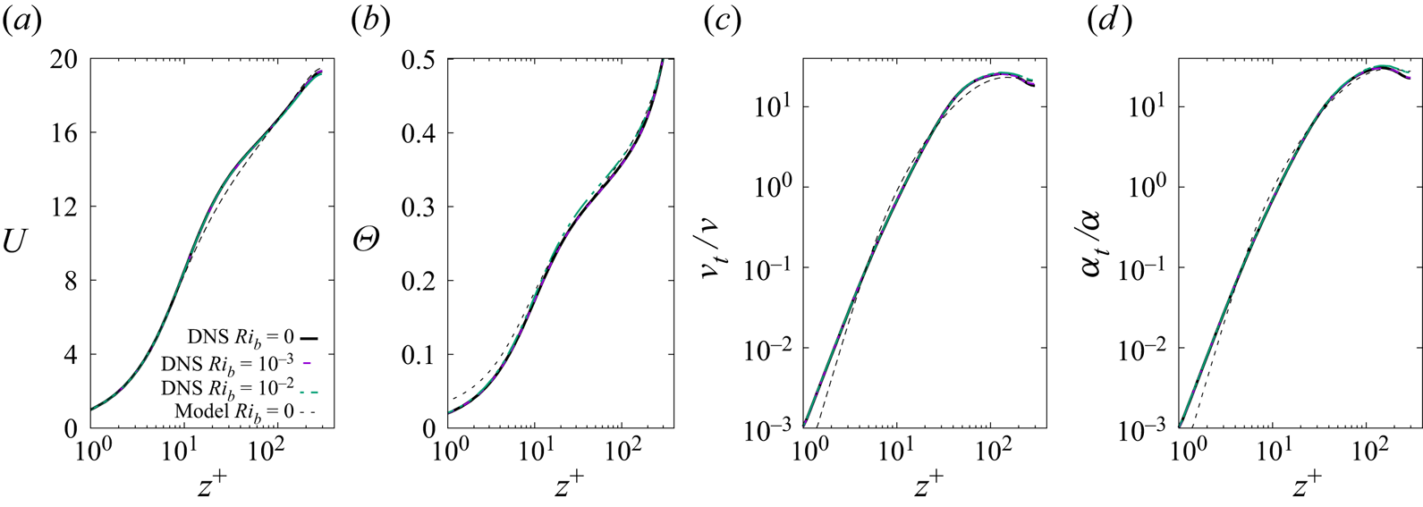
Figure 1. Vertical profiles of the temporally averaged mean streamwise velocity  $U$ (a) and mean temperature $\varTheta$ (b), and of the associated eddy viscosity $\nu _t/\nu$ (c) and thermal eddy diffusivity $\alpha _t/\alpha$ (d). The profiles are issued from DNS data of Pirozzoli et al. (Reference Pirozzoli, Bernardini, Verzicco and Orlandi2017) for $Re_b=10^4$ and $Ri_b=0$ (solid black line), $Ri_b=10^{-3}$ (dashed purple), $Ri_b=10^{-2}$ (dashed-dotted green), and from the extended Cess model computed for the same $Re_b$ and $Ri_b=0$ (dotted black line).
We find that for all the considered cases, the leading eigenvalues correspond to  $k_x=0$ streamwise-uniform modes and have zero imaginary part (not shown). The analysis of the $\sigma (k_y)$ growth rate curves obtained for $k_x=0$ (reported in figure 2 with circular symbols) reveals that while all the modes are linearly stable for $Ri_b=0$ (as is well known already) and $Ri_b=10^{-3}$, an unstable $k_y$ waveband exists for $Ri_b=10^{-2}$, i.e. for the same value of $Ri_b$ where the coherent streamwise rolls are first detected in the DNS, showing that the appearance of these coherent streamwise rolls is associated with a linear instability of $U(z), \varTheta (z)$ to coherent perturbations.
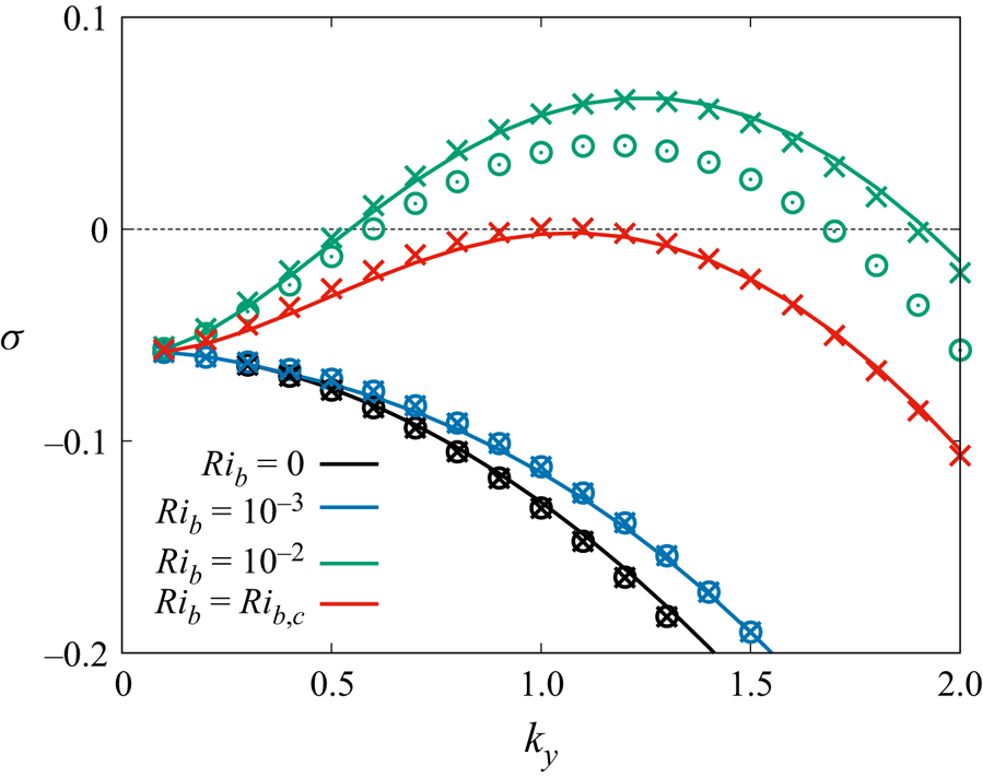
Figure 2. Temporal growth rate  $\sigma$ or the leading normal mode at $Re_b=10^4$ versus the spanwise wavenumber $k_y$ for $k_x=0$ for selected values of $Ri_b$, obtained by making use of DNS mean flow data at the same $Ri_b$ ( $\small \odot$ symbols), DNS mean flow data obtained at $Ri_b=0$ ( $\small \times$ symbols), and the Cess model mean flows (lines).
3.2. Computation of the critical values at $Re_b=10^4$

Additional analysis is necessary to determine the critical Richardson and Rayleigh numbers for the onset of the coherent large-scale convection because the use of DNS mean flow profiles for the stability analysis is limited to only few values of the parameters and, furthermore, is not justified in the supercritical regime where the unstable modes, which have reached finite amplitudes, modify the mean flow profiles. To overcome these difficulties, we therefore introduce two additional approaches.
(i) In a first approach, the stability analysis is performed by changing the value of the Richardson number in the linear operator
$\boldsymbol{\mathsf{A}}$ but using as basic flow profiles the ones obtained by DNS frozen at $Ri_b=0$. This is justified because mean profiles do not change appreciably in subcritical conditions (see figure 1) and are therefore appropriate to detect the onset of the instability.(ii) In the second approach, the linear stability analysis is based on mean profiles provided by the model proposed by Cess (Reference Cess1958), which we have extended to the case of non-uniform temperature, as detailed in Appendix A.


The results obtained with these two approaches are compared in figure 2, from which it can be seen that (a) the two approaches lead to almost indistinguishable growth rates for all  $Ri_b$, and (b) in subcritical conditions, i.e. as long as the growth rates are negative, these growth rates coincide further with those computed in § 3.1 making use of mean flow profiles issued from DNS at the same $Ri_b$. In supercritical conditions, the growth rates computed using the mean flow of the DNS at the same $Ri_b$, where the rolls already affect the mean flow, are slightly smaller than the ones computed on the proper basic flows.
We therefore repeat the stability analysis for a whole set of  $Ri_b$ values by making use of the extended Cess model (second approach) looking for the critical values for the onset of the instability. We find that the critical Richardson number is $Ri_{b,c}=6.47\times 10^{-3}$, which at the considered $Re_b=10^4$ corresponds to the critical Rayleigh number $Ra_c=647\,170$, with the critical spanwise wavenumber $k_{y,c}=1.08$ (see figure 2).
If the first approach is used, where the base flow profiles are the DNS ones ‘frozen’ at  $Ri_b=0$ for the same $Re_b=10^4$, then the critical values $Ri_{b,c}=6.36 \times 10^{-3}$, $Ra_c=636\,889$, $k_{y,c}=1.062$ are found, which are within 2 % of the values computed previously, therefore confirming the accuracy of the linear stability analysis based on the extended Cess model.
The spanwise wavenumber  $k_{y,c}=1.08$ of the critical mode corresponds to the spanwise wavelength $\lambda =5.8$, and the aspect ratio is $A=2.91$ (where
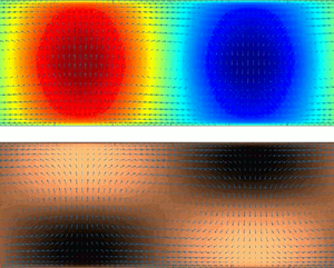
  $A=\lambda /2$ is the ratio of the spanwise wavelength to the channel height). The shape of the critical mode corresponds to the expected coherent convective rolls that induce positive (negative) temperature fluctuations and bottom-wall low-speed (high-speed) streaks in correspondence to the hot updrafts (cold downdrafts), as shown in figure 3.
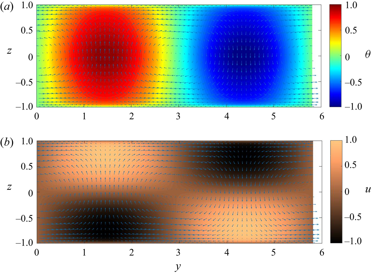
Figure 3. Cross-stream view of the (a) coherent perturbation temperature and (b) streamwise perturbation velocity fields corresponding to the critical mode, with wavenumbers  $k_{x}=0$, $k_y=k_{y,c}$ computed at $Re_b=10^4$ and $Ri_{b,c}$. The associated cross-stream velocity field is reported with arrows. All fields are normalized with respect to their maximum amplitude.
3.3. Relevance of Reynolds stress modelling
To assess the relevance of the inclusion of modelled Reynolds stresses in the linear operator, we have repeated the stability analysis with the quasi-laminar formulation, where it is assumed that  $\nu _t/\nu =0$ and $\alpha _t/\alpha =0$. The critical Richardson number predicted with the quasi-laminar formulation is found to be $Ri_{b,c}=3.82 \times 10^{-5}$, corresponding to the critical Rayleigh number $Ra_c=3816$. These critical values are two orders of magnitude smaller than the ones computed in § 3.2 by including the modelled Reynolds stresses in the formulation, and are not consistent with the DNS of Pirozzoli et al. (Reference Pirozzoli, Bernardini, Verzicco and Orlandi2017), where rolls are not observed for such small values of $Ri_b$ and $Ra$. Furthermore, the critical wavenumber $k_{y,c}=1.56$ predicted with the quasi-laminar approach corresponds to the spanwise wavelength $\lambda =4$ and the aspect ratio $A=2$, which values are half of those observed in the DNS.
Including the effects of turbulent diffusion, which are unaccounted for in the quasi-laminar formulation, is therefore essential in predicting the most basic features of the onset of large-scale convection rolls. We therefore abstain from obtaining further results with the quasi-laminar formulation in the remainder of this investigation.
4. Influence of the Reynolds number on the onset of turbulent convection
After having considered the onset of large-scale convection rolls at the specific Reynolds number  $Re_b=10^4$ in § 3, we now examine the Reynolds number dependence of the critical Richardson and Rayleigh numbers, the critical spanwise wavenumber and the critical mode shape. To this end, we repeat the linear stability analysis for $Pr=1$ and Reynolds numbers ranging from $Re_b = 10^4$ ( $Re_\tau =298$) to $Re_b \approx 10^6$ ( $Re_\tau =20\,000$), which is the largest Reynolds number considered by del Álamo & Jiménez (Reference del Álamo and Jiménez2006), Pujals et al. (Reference Pujals, García-Villalba, Cossu and Depardon2009) and Hwang & Cossu (Reference Hwang and Cossu2010b) in similar linear analyses of turbulent channels with neutral stratification.
4.1. Use of the extended Cess model
For the additional linear stability analyses, performed at higher Reynolds numbers, we make use of base flows based on the extended Cess model. In Appendix A, where this model is described, it is shown that it predicts friction and heat transfer laws  $C_f(Re_b)$, $Nu(Re_b)$ that are in agreement with the DNS results and the semi-empirical fits reported by Pirozzoli et al. (Reference Pirozzoli, Bernardini, Verzicco and Orlandi2017). Remarkably, the agreement with the semi-empirical fits holds at least up to the highest Reynolds number that we consider ( $Re_b\approx 10^6$, $Re_\tau =20\,000$), well beyond the highest Reynolds numbers of the DNS with which they were calibrated (see figure 7 in Appendix A). Furthermore, we have already shown in § 3.2 that linear stability analyses based on the extended Cess model are in agreement with those based on mean profiles issued directly by DNS data at $Re_b=10^4$. These properties provide confidence in the use of the extended Cess model for the stability analyses.
4.2. Dependence of the critical values on the Reynolds number
The additional computations performed for increasing values of the Reynolds number reveal that the critical Richardson number  $Ri_{b,c}$ decreases for increasing Reynolds numbers, from slightly above $0.06$ for $Re_b=10^4$, to slightly above $0.02$ for $Re_b=10^6$, as shown in figure 4(a). The corresponding critical Rayleigh number $Ra_c=Ri_{b,c}\,Pr \, Re_b^2$ increases with the Reynolds number approximately as $Ra_c=0.04\,Re_b^{1.8}$, reaching values higher than $10^9$ for the highest considered Reynolds numbers (see figure 4b).
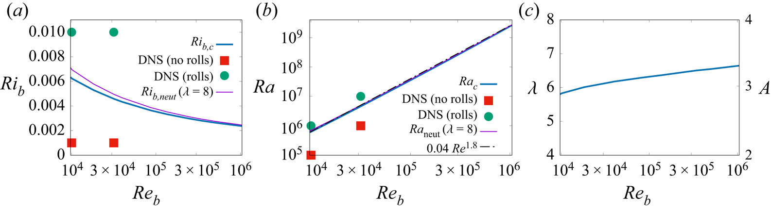
Figure 4. Critical parameters dependence on Reynolds number  $Re_b$: (a) critical Richardson number $Ri_{b,c}$; (b) critical Rayleigh number $Ra_{c}$; and (c) critical wavelength $\lambda =2 {\rm \pi}/ k_{y,c}$. In (a,b), the critical curves (blue solid lines) and the neutral parameters of disturbances with $\lambda =8$ (purple solid lines) are compared to the DNS findings of Pirozzoli et al. (Reference Pirozzoli, Bernardini, Verzicco and Orlandi2017), where coherent large-scale rolls have disappeared (filled red square symbols), and those where they are first detected (filled green circle symbols). The best fit to the $Ra_c(Re_b)$ curve is also reported in (b) (black dashed-dotted line). In (c), the results are also reported in terms of the aspect ratio $A=\lambda /2$ (the ratio of the critical mode spanwise wavelength to the channel height).
The spanwise wavelength  $\lambda$, expressed in units of domain half-height $h$, and the aspect ratio $A=\lambda /2$ of the critical modes increase slightly with the Reynolds number from $\lambda =5.82$ ( $A=2.9$) for $Re_b=10^4$, to $\lambda =6.55$ ( $A=3.27$) for $Re_b=10^6$. This spanwise wavelength is, however, smaller than the $\lambda =8$ spanwise wavelength ( $A=4$) of the large-scale rolls that first emerge in the DNS of Pirozzoli et al. (Reference Pirozzoli, Bernardini, Verzicco and Orlandi2017). We ascribe this difference to the fact that the spanwise size of the numerical domain used in the DNS is $L_y=8h$, and therefore only structures with $\lambda =8$ ( $A=4$) or $\lambda =4$ ( $A=2$) can be resolved at the largest scales in the DNS, where periodic boundary conditions are enforced in the spanwise direction. To validate further our results with respect to those of the DNS, we have therefore computed additionally the neutral Richardson and Rayleigh numbers corresponding to perturbations with $\lambda =8$ observed in the DNS. As shown in figure 4, the computed neutral Richardson and Rayleigh numbers at which coherent modes with $\lambda =8$ become unstable are extremely similar to the critical ones.
Even more importantly, both the computed critical curves and those corresponding to  $\lambda =8$ are consistent with the DNS results of Pirozzoli et al. (Reference Pirozzoli, Bernardini, Verzicco and Orlandi2017), lying between the $Ri_b$ (and $Ra$) values where coherent large-scale rolls are first observed (filled green circle symbols in the figure) and those where they first disappear (filled red square symbols) in the DNS, as shown in figure 4.
4.3. Use of the friction Richardson number
The very large values attained by the critical Rayleigh numbers for increasing Reynolds numbers can be attributed to the decreasing values of the viscosity  $\nu$ and thermal diffusivity $\alpha$, both appearing in the denominator of $Ra$. An effective Rayleigh number $Ra_{eff} = 8 h \beta \, \Delta \varTheta / (\overline {\nu }_{T}\overline {\alpha }_{T})$ can be defined based on the wall-normal-averaged total viscosity $\overline {\nu }_{T}=(1/2)\int _{-1}^1 \nu _T(z)\,{\rm d} z$ and the similarly defined $\overline {\alpha }_{T}$. In figure 5(a), it is shown that the critical value of this effective Rayleigh number remains in the range $Ra_{eff,c} \approx 1200\unicode{x2013}1300$ for almost all the considered $Re_b$.
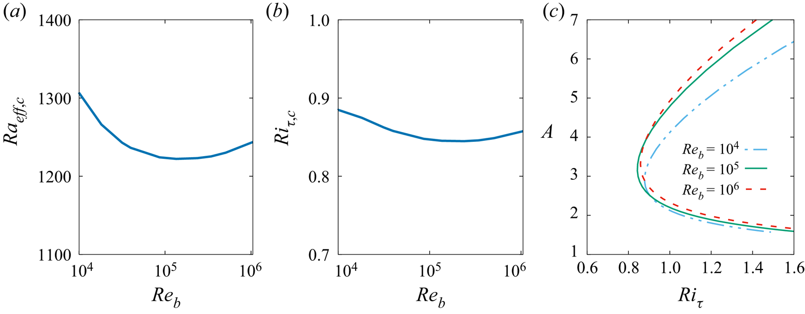
Figure 5. Critical parameters dependence on Reynolds number  $Re_b$: (a) critical effective Rayleigh number $Ra_{eff,c}$; (b) critical friction Richardson number $Ri_{\tau,c}$. In (c) are reported the neutral curves $Ri_{\tau,neut}(A)$ for the selected Reynolds numbers $Re_b=10^4$, $1.35 \times 10^5$ and $1.08 \times 10^6$.
As  $\nu _t$ and $\alpha _t$ are, in a first approximation, both proportional to $Re_\tau$ (see e.g. (A1) and (A2)), the effective Rayleigh number behaves approximately like $Ra / Re_\tau ^2$. Recalling that $Ra =8\,Ri_\tau \,Pr \, Re_\tau ^2$, it appears that using $Ra_{eff}$ is almost equivalent to using the friction Richardson number $Ri_\tau$. Indeed, as shown in figure 5(b), the critical value of the friction Richardson number remains near $Ri_{\tau,c} = 0.86$ within ${\pm }3\,\%$ accuracy for all the considered Reynolds numbers. The instability threshold is therefore best defined in terms of $Ri_\tau$. Furthermore, neutral curves expressed in terms of $Ri_\tau$ are less sensitive to the Reynolds number for the highest Reynolds numbers, as shown in figure 5(c).
4.4. Critical modes shapes
The vertical profiles associated with the critical modes computed for selected Reynolds numbers are reported in figure 6. Critical modes, being eigenfunctions of a linear operator, are defined up to an arbitrary constant. In order to compare the different profiles pertaining to the different considered Reynolds numbers, the arbitrary constant is chosen such that the maximum vertical velocity is equal to 1 for all cases. From figure 6(a), it can be seen that the profile of the vertical velocity component  $\hat {w}(z)$ of the coherent critical mode is nearly sinusoidal, and its shape is insensitive to the Reynolds number. On the contrary, the temperature $\hat {\theta }(z)$ and streamwise velocity $\hat {u}(z)$ profiles are characterized by strong gradients near the walls, as shown in figures 6(b,c). Their maximum amplitudes do slightly increase with the Reynolds number, probably reflecting a slightly increasing non-normality of the linear operator $\boldsymbol{\mathsf{A}}$ (see e.g. Cossu et al. Reference Cossu, Pujals and Depardon2009; Pujals et al. Reference Pujals, García-Villalba, Cossu and Depardon2009; Hwang & Cossu Reference Hwang and Cossu2010b).
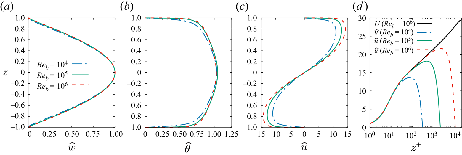
Figure 6. Vertical profiles of the critical modes (coherent perturbations) computed for the selected Reynolds numbers  $Re_b=10^4$, $1.35 \times 10^5$ and $1.08\times 10^6$: (a) coherent vertical velocity $\hat {w}(z)$, (b) temperature $\hat {\theta }(z)$, and (c) streamwise velocity $\hat {u}(z)$. In (d), the streamwise velocity critical mode profiles $\hat {u}(z^+)$ are replotted against the wall units coordinate $z^+$, properly rescaled, to show their proportionality to the mean flow profile $U(z^+)$ in the inner layer.
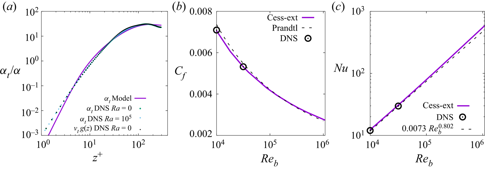
Figure 7. Comparison of the extended Cess model relative eddy thermal diffusivity  $\alpha _t/\alpha$ to DNS data and to the DNS rescaled eddy viscosity $g(z)\,\nu _t/\nu$ for $Re_b=10^4$ (a). The extended Cess model (purple solid lines) friction coefficient $C_f=2 u_\tau ^2 / u_b^2$ (b) and Nusselt number $Nu$ (c) dependence on $Re_b$ are compared to DNS data (symbols) and to the associated semi-empirical laws (black dotted lines) reported by Pirozzoli et al. (Reference Pirozzoli, Bernardini, Verzicco and Orlandi2017).
We also find that the streamwise velocity profiles of the critical mode are proportional to the mean velocity profile from the wall to at least the end of the logarithmic layer ( $z^+/Re_\tau \approx 0.1$), as shown in figure 6(d). These coherent perturbation profiles, therefore, also embed a viscous sublayer, a buffer layer and a logarithmic layer similarly to what was found for optimally forced coherent streaks in the absence of heating (Cossu et al. Reference Cossu, Pujals and Depardon2009; Pujals et al. Reference Pujals, García-Villalba, Cossu and Depardon2009). Furthermore, the streamwise velocity component of the critical mode reaches at least 50 % of its maximum amplitude in the buffer layer, confirming the large influence that non-universal large-scale coherent structures have on the near-wall dynamics.
5. Conclusions
The main goal of this study was to understand if a suitable linear stability analysis could explain the onset of large-scale convection rolls observed in wall-bounded turbulent shear flows exposed to destabilizing temperature gradients, and predict the threshold where instability sets in and the aspect ratio of the rolls at the instability onset. A second goal was to assess the relative merits of including or not modelled Reynolds stresses in the linear stability operator motivated by the current ambiguities in the formulation of linear analyses of turbulent flows.
To these ends, we have examined the linear stability of mean flow profiles in a pressure-driven turbulent channel flow for Reynolds numbers ranging from  $Re_b=10^4$ to $Re_b \approx 10^6$ ( $Re_\tau$ ranging from $298$ to $20\,000$), and Rayleigh numbers ranging from $Ra=0$ to more than $Ra=10^9$. The stability of the mean flows with respect to coherent perturbations has been assessed by including the effect of Reynolds stresses in the linear operator, extending the approach of Reynolds & Hussain (Reference Reynolds and Hussain1972) to the thermally stratified case. The main results can be summarized as follows.
(i) The onset of large-scale rolls can be associated with the linear instability of the turbulent mean flow to coherent perturbations.
(ii) The linear instability sets in at critical friction Richardson numbers
$Ri_{\tau,c}=0.86 \pm 0.026$ for the considered range of Reynolds numbers (where $Ri_\tau$ is assumed positive in the unstably stratified case). This corresponds to critical Rayleigh numbers increasing with the Reynolds number as $Ra_c \approx 0.04Re_b^{1.8}$. These critical values are consistent with what was observed in DNS by Pirozzoli et al. (Reference Pirozzoli, Bernardini, Verzicco and Orlandi2017).(iii) The aspect ratio of the critical rolls is in the range
$A \approx 2.9\unicode{x2013}3.3$ (spanwise wavelengths $\lambda \approx 5.8\unicode{x2013}6.6$ when expressed in channel half-height units) for the considered Reynolds numbers.(iv) The vertical velocity profiles of the critical mode are not sensitive to the Reynolds number and are nearly sinusoidal, while those of the temperature and the streamwise velocity display large gradients near the walls, which increase slightly with the Reynolds number.
(v) The streamwise velocity profiles of the critical modes are proportional to the turbulent mean flow profile from the wall to the logarithmic layer, and reach 50 % of their maximum amplitude in the buffer layer.
(vi) It is necessary to include modelled Reynolds stresses in the linear operator to obtain realistic values of the critical parameters.


These results, by providing predictions consistent with DNS in a well-defined setting, show that a suitable linear stability analysis is able to predict the onset of large-scale convection in turbulent wall-bounded flows and that coherent large-scale rolls are unstable linear modes sustained by the unstably stratified turbulent mean flow. The existence of such a linear instability with well-defined thresholds is consistent with the DNS of turbulent channels by Pirozzoli et al. (Reference Pirozzoli, Bernardini, Verzicco and Orlandi2017) and the large-eddy simulations of atmospheric boundary layers by Jayaraman & Brasseur (Reference Jayaraman and Brasseur2021), which show that a well-defined finite heating threshold exists for the onset of large-scale rolls. Previous ‘local’ interpretations of the interaction of unstable stratification with shear-induced turbulent coherent streaks, such as that of Khanna & Brasseur (Reference Khanna and Brasseur1998), explain why low-speed streaks on the ground act as the seeds of thermal updrafts but could not explain and predict straightforwardly that a well-defined threshold exists for the onset of the large-scale coherent rolls, or predict the associated critical Rayleigh or Richardson numbers or the rolls aspect ratio. The strength of the linear stability analysis that we have used therefore resides in the fact that it addresses directly the interaction of the coherent large-scale rolls with the turbulent mean flow, while also including, via the eddy diffusivities, the effects of nonlinear energy transfers with other shear-induced and buoyancy-induced structures (which lead finally to dissipation). This ‘global’ point of view is therefore able to reproduce the physics explained by the local interpretations (e.g. that hot updrafts corresponds to ground low-speed streaks, as seen in figure 3), while being at the same time able to quantify exactly global properties, such as the growth rate of large-scale rolls and the most amplified aspect ratios, as functions of the Reynolds and Richardson (or Rayleigh) numbers.
The onset of large-scale convection rolls at finite values of the Rayleigh (or Richardson) number and the fact that it is associated with a linear instability are clearly reminiscent of the Rayleigh–Bénard instability in a laminar background. Despite their apparent similarities, however, we find that the laminar and turbulent flow cases are very different. In the laminar case, indeed, the Rayleigh–Bénard instability developing on top of the laminar Poiseuille flow onsets at a fixed critical Rayleigh number ( $Ra_c=1708$ for no-slip conditions on both walls) that does not depend on the Reynolds number of the underlying Poiseuille flow (see e.g. Gage & Reid Reference Gage and Reid1968; Jerome et al. Reference Jerome, Chomaz and Huerre2012). In the turbulent case, on the contrary, the critical Rayleigh numbers increase significantly with Reynolds numbers because higher buoyancy power is necessary to overcome the increasingly high turbulent diffusion when the Reynolds number is increased. In the turbulent case, indeed, the relevant critical parameter is the friction Richardson number $Ri_\tau$ that compares these two effects and that we find to be almost independent of the Reynolds number, at least for the considered $Re_b$ ranging from $10^4$ to $10^6$. Also, while in the laminar case the aspect ratio of the critical Rayleigh–Bénard rolls does not change with the Reynolds number, in the turbulent case it does slightly increase with the Reynolds number because of the increasing turbulent eddy diffusivities.
The presented results, of course, have some limitations. The most important one probably is that only very few numerical or experimental results exist to which it is possible to compare the predictions of the linear stability analysis. The most recent and useful results that we are aware of are the DNS of Pirozzoli et al. (Reference Pirozzoli, Bernardini, Verzicco and Orlandi2017) for which data for the onset of large-scale rolls are available up to  $Re_b=3.16\times 10^{4}$, and with simulated $Ra$ and $Ri_b$ values all spaced by a decade and only for numerical domains of spanwise aspect ratio $A=4$. Therefore, despite the fact that our predictions are consistent with the existing DNS results of of Pirozzoli et al. (Reference Pirozzoli, Bernardini, Verzicco and Orlandi2017), additional numerical and/or experimental studies with a more dense spacing of $Ra$ and $Ri_b$ values, extending to higher Reynolds numbers and with additional aspect ratios of the numerical domain, would certainly allow for a more precise quantitative assessment of the critical Rayleigh (or Richardson) numbers and the critical rolls aspect ratios predictions presented here.
Concerning the modelling of Reynolds stresses, the presented analysis is based on an extension of the closure of Reynolds & Hussain (Reference Reynolds and Hussain1972), which represent Reynolds stresses by means of an isotropic eddy viscosity corresponding to the temporally averaged mean flow, to the case of non-neutral stratifications by means of the definition of a thermal eddy diffusivity corresponding to the mean temperature profile. This is probably the simplest possible model that allows us to take into account inter-scale energy transfers. The simplicity of the model is an advantage for the interpretation of the results because it requires only the knowledge of the temporally averaged mean velocity and temperature vertical profiles. However, it represents also a potential limitation if more precise quantitative predictions are sought. For the goals of this study, nevertheless, this simple model has proven effective probably because the most amplified modes have large spatial scales (they are streamwise-uniform and have large spanwise wavelengths) and are quasi-steady (temporal eigenvalues have zero imaginary part). More sophisticated models might be necessary in less favourable situations, such as e.g. to predict the onset of the rolls meandering that has not been addressed in the present investigation.
As already mentioned, a second goal of this investigation was to compare the performance of the statistical-linear approach (discussed above) to that of the quasi-laminar approach in a setting where no modelling of an external forcing is needed. We find that the quasi-laminar stability analysis, where modelled Reynolds stresses are not included in the linear operator, leads to a strong underestimation (by two orders of magnitude) of the critical Rayleigh and Richardson numbers, as well as predicting critical rolls aspect ratios typical of the laminar case. The results of the present investigation therefore represent additional evidence of the appropriateness of the statistical-linear approach introduced by Reynolds & Hussain (Reference Reynolds and Hussain1972) to describe the dynamics of averaged (coherent) perturbations of the temporally averaged mean flow. This type of approach, indeed, is able to predict the amplification of large-scale coherent structures in turbulent channel flows in both the unstably stratified case, via the modal stability analysis performed in this study, and the neutrally stratified case, by means of non-modal analyses (see e.g. del Álamo & Jiménez Reference del Álamo and Jiménez2006; Pujals et al. Reference Pujals, García-Villalba, Cossu and Depardon2009; Hwang & Cossu Reference Hwang and Cossu2010b; Morra et al. Reference Morra, Semeraro, Henningson and Cossu2019).
The approach taken in this study can probably be extended straightforwardly to the case of the unstably stratified atmospheric boundary layer by including the effect of Coriolis acceleration, ground roughness and capping inversions. In this context, the predictions of this type of linear stability analysis could be tested against the currently unexplained findings of Jayaraman & Brasseur (Reference Jayaraman and Brasseur2021), who report the onset of roll-like structures for values of ground heating much lower than those commonly associated with even moderately convective regimes. Another extension of the present approach will consist in the inclusion of nonlinear terms in the formulation in order to access finite-amplitude solutions of the rolls that exist above the critical Rayleigh/Richardson thresholds and to be able to compare directly the finite-amplitude solutions to direct numerical simulation results and predict their secondary instability leading to their meandering motions. These extensions are under current intensive investigation.
Funding
This research received no specific grant from any funding agency, commercial or not-for-profit sectors.
Declaration of interests
The author reports no conflict of interest.
Data availability statement
The data that support the findings of this study are available from the author.
Appendix A. The extended Cess model for the mean flow
In this appendix, we describe the model that is used in a substantial part of this study to approximate the eddy diffusivities and the associated mean flow profiles. The semi-empirical expression proposed by Cess (Reference Cess1958), as reported by Reynolds & Tiederman (Reference Reynolds and Tiederman1967), is assumed for the eddy (kinematic) viscosity  $\nu _t$:
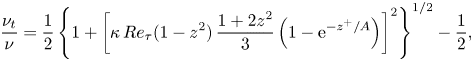 \begin{equation} \frac{\nu_{t}}{\nu} = \frac{1 }{2} \left\{1+\left[{\kappa\,Re_\tau}(1-z^2)\, \frac{1+2z^2}{3}\left(1-{\rm e}^{{-}z^+{/} A}\right) \right]^2\right\}^{1/2}-\frac{1}{2}, \end{equation}
where  $z^+=Re_\tau (1-|z|)$, and the values of the von Kármán constant $\kappa =0.426$ and $A=25.4$ are based on best fits to the DNS at $Re_\tau =2000$ of Hoyas & Jiménez (Reference Hoyas and Jiménez2006). The mean velocity profile is obtained by integrating ${\rm d} U/{\rm d} z=-Re_\tau \,z/(1+\nu _t/\nu )$, a relation derived from the mean momentum budget equation (Reynolds & Tiederman Reference Reynolds and Tiederman1967; Pope Reference Pope2000). As shown in figure 1, the Cess model provides reasonable approximations for $U$ and $\nu _t$, and has already been used widely for stability analyses of turbulent mean flows (see, among others, Reynolds & Tiederman Reference Reynolds and Tiederman1967; Waleffe, Kim & Hamilton Reference Waleffe, Kim and Hamilton1993; Farrell & Ioannou Reference Farrell and Ioannou1996; del Álamo & Jiménez Reference del Álamo and Jiménez2006; Pujals et al. Reference Pujals, García-Villalba, Cossu and Depardon2009; Hwang & Cossu Reference Hwang and Cossu2010b; Morra et al. Reference Morra, Semeraro, Henningson and Cossu2019). We have verified further that the friction law $C_{f}(Re_b)$ associated Cess model is in good agreement with Prandtl's law used by Pirozzoli et al. (Reference Pirozzoli, Bernardini, Verzicco and Orlandi2017), even at Reynolds numbers much higher than those accessed in their DNS, as shown in figure 7(b).
We have extended the Cess model to include the effect of turbulent heat transport (temperature diffusion) in the forced convection regime preceding the onset of large-scale convection (we restrain to the  $Pr=1$ value considered in this study). In this regime, where the temperature behaves as a passive scalar, empirical trial and error tests show that in the bulk of the flow, DNS data verify $\alpha _t \approx g(z)\,\nu _t$, where $g(z)=(1-\chi z^2)/(1-\chi )$ with $\chi \approx 0.25$. We have therefore modelled the thermal eddy diffusivity by including $g(z)$ in Cess's law:
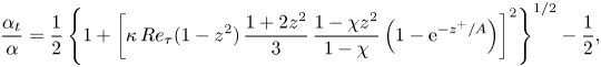 \begin{equation} \frac{\alpha_{t}}{\alpha} = \frac{1}{2} \left\{1+\left[{\kappa\,Re_\tau}(1-z^2)\,\frac{1+2z^2}{3}\, \frac{1-\chi z^2}{1-\chi}\left(1-{\rm e}^{{-}z^+{/} A}\right) \right]^2\right\}^{1/2}-\frac{1}{2}, \end{equation}
using the same constants  $\kappa$, $A$ used in (A1), and $\chi =0.25$. The temperature field can be retrieved from ${\rm d}\varTheta /{\rm d} z = - Re_\tau \,Q / [Pr\,(1+\alpha _t/\alpha )]$, a relation derived from the mean energy budget. The model's temperature field and eddy diffusivity fit the DNS data reasonably well, as shown in figures 1(a,b) and figure 7(a). We show further in figure 7(c) that the $Nu(Re_b)$ curve associated with the extended Cess model equation (A2) is in good agreement with the DNS of Pirozzoli et al. (Reference Pirozzoli, Bernardini, Verzicco and Orlandi2017) and their empirical fit $Nu = 0.0073\,Re_b^{0.802}$, even at Reynolds numbers much higher than those accessed in their DNS.


 Open access