


1. Introduction
The flow of two immiscible fluids is often encountered in the petroleum industry, where crude oil and water, upon extraction from wells, are transported over very long distances and finally separated in designated process plants. When oil and water flow together inside horizontal pipelines and channels, different flow regimes are possible. At low flow rates, the flow is stratified and the oil–water interface is smooth. At moderate flow rates, the flow can still remain stratified, but the oil–water interface is characterised by the presence of waves, which are initially long compared with the pipe diameter/channel height, and become shorter as the flow rate is increased. At even higher flow rates, waves might break and generate a dispersed flow in which water drops form inside the oil layer and/or oil drops form inside the water layer (Al Wahaibi & Angeli Reference Al Wahaibi and Angeli2011; Barral & Angeli Reference Barral and Angeli2013).
Owing to the inherent modelling complexity of the flow, literature in the field of oil–water transportation inside pipes and channels is almost entirely based on experimental investigations, focused mainly on the evaluation of flow regimes/global flow properties such as pressure drop and flow rate (Sotgia, Tartarini & Stalio Reference Sotgia, Tartarini and Stalio2008), and on single-point measurements of the interface deformation (Issenmann, Laroche & Falcon Reference Issenmann, Laroche and Falcon2016), but also on analytical investigations of flow stability (Barmak et al. Reference Barmak, Gelfgat, Ullmann, Brauner and Vitoshkin2016, Reference Barmak, Gelfgat, Ullmann and Brauner2019).
More detailed experimental observations, aiming at characterising the flow structure and the interface deformation, have become possible in recent years, thanks to the development of laser-based diagnostic techniques such as planar laser-induced fluorescence (PLIF) and particle image velocimetry (PIV)/particle tracking velocimetry (PTV). In particular, PLIF provides information on the scalar distribution of the two phases in the plane of the laser light, whereas PIV/PTV can provide the corresponding instantaneous velocity distribution. These techniques are generally applied to cases in which the two fluids have the same refractive index (RI) (Conan et al. Reference Conan, Masbernat, Décarre and Line2007; Morgan et al. Reference Morgan, Markides, Zadrazil and Hewitt2013), in order to minimise the optical distortion at the liquid–liquid interface. Similar techniques have also been applied to gas–liquid systems, including horizontal stratified air–water flow in pipes (Ayati et al. Reference Ayati, Kolaas, Jensen and Johnson2014, Reference Ayati, Kolaas, Jensen and Johnson2015, Reference Ayati, Kolaas, Jensen and Johnson2016) and even gas–liquid annular flow (Zadrazil & Markides Reference Zadrazil and Markides2014). Very recently, a new simultaneous two-line (two-colour) technique, combining PLIF and PIV/PTV for non-RI-matched fluids, has been developed (Ibarra et al. Reference Ibarra, Zadrazil, Matar and Markides2018; Ibarra, Matar & Markides Reference Ibarra, Matar and Markides2021), and is expected to contribute further to the research in the field.
Given the difficulties in obtaining accurate experimental results of interfacial flows, time and space-resolved numerical simulations, although complex and computationally expensive to perform, are a valuable tool to provide insightful measurements of the entire flow field and to offer a corresponding precise characterisation of the liquid–liquid interface deformation. Compared with the case of gas–liquid flows, in which the number of accurate simulations is rapidly increasing (Popinet Reference Popinet2018), the case of liquid–liquid flows has gathered relatively less interest, which is however currently rising thanks to the renewed interest in the water-lubricated oil pipelines (Xie et al. Reference Xie, Zheng, Triantafyllou, Constantinides, Zheng and Karniadakis2017; Kim & Choi Reference Kim and Choi2018). In a series of previous studies (see Ahmadi et al. Reference Ahmadi, Roccon, Zonta and Soldati2018; Roccon, Zonta & Soldati Reference Roccon, Zonta and Soldati2019, Reference Roccon, Zonta and Soldati2021), we have performed computations, based on pseudo-spectral direct numerical simulations (DNS) of turbulence coupled with a phase field method (PFM), to study the dynamics of the liquid–liquid flow moving inside a plane channel. However, to the best of the authors’ knowledge, a detailed space–time characterisation of the liquid–liquid interface in such a configuration is not yet available. This is exactly the aim of the present work. We consider two immiscible fluid layers that move, under the action of an imposed mean pressure gradient, inside a plane channel. The two fluid layers have same thickness and same density, but different viscosity. As in our previous studies, we combine pseudo-spectral DNS of turbulence with PFM to track the dynamics of the liquid–liquid interface. Upon application of space and time-resolved flow measurements, we are able to compute the spectral properties of the liquid–liquid interface and discuss them in the context of wave turbulence theory (WTT) (Zakharov & Filonenko Reference Zakharov and Filonenko1967; Zakharov, L'vov & Falkovich Reference Zakharov, L'vov and Falkovich1992; Newell & Rumpf Reference Newell and Rumpf2011; Falcon & Mordant Reference Falcon and Mordant2022).
It is important to note that the waves that form in a stratified oil–water system are extremely interesting also from a fundamental viewpoint: due to the similar density of the two fluids, the influence of gravity is ruled out and the entire evolution of the interfacial waves is dominated by surface tension. This represents a convenient numerical set-up, which gives us the possibility to challenge current understanding of capillary waves propagation (Longuet-Higgins Reference Longuet-Higgins1963; Phillips Reference Phillips1977). Obtaining similar results with larger density difference fluids would otherwise require complex experimental measurements to be performed in microgravity conditions (Berhanu et al. Reference Berhanu, Falcon, Michel, Gissinger and Fauve2019).
2. Methodology
2.1. Computational method
We consider two immiscible fluid layers flowing inside a rectangular channel under the effect of a constant mean pressure gradient. The channel has dimensions  $L_x=8{\rm \pi} h$, $L_y=2 {\rm \pi}h$ and $L_z=2h$, along the streamwise ( $x$), spanwise ( $y$) and wall-normal ( $z$) directions, respectively. The two layers have the same thickness, so that the initially undeformed interface is located at a distance $h$ both from the top and from the bottom wall, and same density, $\rho _1=\rho _2=\rho$, but different viscosity, $\mu _1\ne \mu _2$ (and, hence, different kinematic viscosity, $\nu _1\ne \nu _2$). The interface between the two fluids has a constant and uniform surface tension
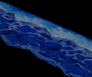
  $\sigma$. A sketch of the domain geometry, along with an instantaneous visualisation of the interface topology is provided in figure 1. To describe the dynamics of the two-phase flow system, we use a PFM. This method is based on the introduction of an order parameter $\phi$ that is uniform in the bulk phases ( $\phi =+1$ in one phase, and $\phi =-1$ in the other phase), whereas it varies continuously over the interface separating the two phases. Using the half-channel height, $h$, as the characteristic length scale, and the shear velocity, $u_\tau =\sqrt {\tau _w/\rho }$ (with $\tau _w$ the shear stress at the channel wall), as characteristic velocity, the governing equations (Navier–Stokes and Cahn–Hilliard) can be expressed in non-dimensional form as follows:
 \begin{gather} \boldsymbol{\nabla} \boldsymbol{\cdot} \boldsymbol{u} = 0, \end{gather}
 \begin{gather}\frac{\partial \boldsymbol{u}}{\partial t} + \boldsymbol{u} \boldsymbol{\cdot} \boldsymbol{\nabla} \boldsymbol{u} ={-} \boldsymbol{\nabla} {p} + \frac{1}{Re_\tau} \boldsymbol{\nabla} \boldsymbol{\cdot} [\mu(\phi, \mu_r) (\boldsymbol{\nabla} \boldsymbol{u} + \boldsymbol{\nabla} \boldsymbol{u}^T )] + \frac{3}{\sqrt{8}} \frac{Ch}{We} \boldsymbol{\nabla} \boldsymbol{\cdot} \boldsymbol{T}_{\boldsymbol{c}}, \end{gather}
 \begin{gather}\frac{\partial {\phi}}{\partial t} + \boldsymbol{u} \boldsymbol{\cdot} \boldsymbol{\nabla} \phi = \frac{1}{Pe} \nabla^2 (\phi^3 - \phi - Ch^2 \nabla^2 \phi), \end{gather}
where  $\boldsymbol {u}=(u,v,w)$ is the velocity vector and $\boldsymbol {\nabla } p$ is the pressure gradient (whose mean value is set to $\overline {\boldsymbol {\nabla } p}=-1$), whereas $\mu _r={\mu _1}/{\mu _2}$ is the viscosity ratio. The term $\mu (\phi,\mu _r)$ defines the non-dimensional viscosity distribution inside the domain (Ding, Spelt & Shu Reference Ding, Spelt and Shu2007; Kim Reference Kim2012), whereas the term $3Ch/( \sqrt {8} We) \boldsymbol {\nabla } \boldsymbol {\cdot } \boldsymbol {T}_{\boldsymbol {c}}$ represents the capillary force per unit mass due to surface tension, with $\boldsymbol {T}_{\boldsymbol {c}} = |\boldsymbol {\nabla } \phi |^2 \boldsymbol {I} - \boldsymbol {\nabla } \phi \otimes \boldsymbol {\nabla } \phi$. The following dimensionless numbers appear in the equations: the shear Reynolds number, $Re_\tau =\rho u_\tau h/ \mu _2$, which is the ratio between inertial and viscous forces (computed using the viscosity of the more viscous layer, $\mu _2$, as a reference); the Weber number, $We=\rho u_\tau ^2 h /\sigma$, which is the ratio between inertial and surface tension forces; the Péclet number, $Pe = u_\tau h / \mathcal {M} \beta$, which is a parameter that controls the interface relaxation time and is defined in terms of the Onsager coefficient, or mobility, $\mathcal {M}$, and of an additional numerical coefficient, $\beta$, used in the non-dimensionalisation of the Cahn–Hilliard equation; and, finally, the Cahn number, $Ch = \xi /h$, which represents the dimensionless extension of the transition layer between the two phases (whose dimensional value is $\xi$). The governing equations are discretised using a pseudo-spectral method, based on transforming the field variables into wavenumber space via Fourier representations in the periodic (homogeneous) directions, $x$ and $y$, and Chebyshev representation in the wall-normal (non-homogeneous) direction, $z$. Periodicity along $x$ and $y$ is assumed for both velocity $\boldsymbol {u}$ and order parameter $\phi$, whereas no-slip ( $\boldsymbol {u}$) and no-flux ( $\phi$) conditions are imposed at the two walls. Further details on the numerical method can be found in Soligo, Roccon & Soldati (Reference Soligo, Roccon and Soldati2019, Reference Soligo, Roccon and Soldati2021).

Figure 1. Sketch of the computational domain. Two immiscible fluid layers, with viscosity  $\mu _1$ (upper layer) and $\mu _2$ (lower layer) flow inside a plane channel under the action of an imposed pressure gradient. The instantaneous liquid–liquid interface deformation is shown in white.
2.2. Simulation set-up
We consider two different cases. Both cases are characterised by the same value of the reference shear Reynolds number,  $Re_\tau =300$, and Weber number, $We=1.0$. The viscosity ratio between the two fluids is $\mu _r=1.00$ for the first case and $\mu _r=0.25$ for the second case. The values of the physical parameters are chosen to mimic a situation in which a light industrial oil (Exxon Mobil Solvesso 200 ND) with $\rho = 980 {\rm kg}\ {\rm m}^{-3}$, $\mu _2 = 3.85 \times 10^{-3}\ {\rm Pa}\ {\rm s}$ and $\sigma = 0.044\ {\rm N}\ {\rm m}^{-1}$ flows together with water inside a channel of height $2h = 6 \times 10^{-2}$ m, at a reference shear velocity of $u_\tau = 3.8 \times 10^{-2} \ {\rm ms}^{-1}$. Note that the reduction of the viscosity in the upper layer leads to a corresponding increase of the local Reynolds number, which can be estimated as $Re_{\tau,loc} \simeq Re_{\tau }/\mu _r$ (Roccon et al. Reference Roccon, Zonta and Soldati2021). As a consequence, the number of grid points $N_x \times N_y \times N_z$ must increase for decreasing $\mu _r$, in order to maintain a suitable resolution. To ensure a correct representation of the interface dynamics, all simulations are run for $Ch=0.02$ and $Pe =3/Ch=150$ (Jacqmin Reference Jacqmin1999). For both simulations, the initial condition is taken from a preliminary simulation of a single phase flow at $Re_{\tau }=300$, on top of which we properly define the initial distribution of the phase field $\phi$ so that the liquid–liquid interface is at the beginning flat and located at the channel centre. The main simulation parameters are summarised intable 1.
Table 1. Overview of the main simulation parameters.

3. Results
3.1. Statistics of the turbulent flow field
We first look at the flow statistics for the different cases considered in this work. In figure 2, we show the mean streamwise velocity,  $\langle u (z)/u_\tau \rangle$, as a function of the wall-normal coordinate. Results for the two-layers configuration at different viscosity ratio ( $\mu _r=1.00$ and $\mu _r=0.25$) are shown together with the reference single-phase (SP) case. When the two layers have the same viscosity ( $\mu _r=1.00$), the mean velocity profile is only slightly modified by the presence of the liquid–liquid interface. However, when the upper layer has a lower viscosity ( $\mu _r=0.25$) the mean streamwise velocity is consistently increased, and its shape much more modified. This reflects into an overall flow rate increase of about $11\,\%$ (see table 2), which can be traced back to a corresponding drag reduction (because our simulations are all run at the same pressure gradient). Note also that the location at which the streamwise velocity has a maximum (represented by the dashed horizontal lines in figure 2) is changed. In particular, for $\mu _r=0.25$, the maximum is shifted upwards with respect to the channel centre, and indicates the tendency for the streamwise velocity profile to be skewed when the two layers have different viscosity.

Figure 2. Mean streamwise velocity profiles,  $\langle u (z)/u_\tau \rangle$, as a function of the wall-normal distance $z/h$, for the three different cases: $\mu _r=1.00$ (blue line), $\mu _r=0.25$ (green line), single phase flow (SP, black line). Also shown (horizontal dashed lines, $z_{u_{max}}$) is the location at which the mean streamwise velocity profiles have a maximum.
Table 2. Mean flow rates for the different simulations. Here  $Q_1$, $Q_2$ and $Q_{t}$ correspond to the mean flow rates of the upper layer (oil), the lower layer (water) and the total mean flow rate over the whole channel height, respectively, whereas $Q_{SP}$ is the mean flow rate of the reference single phase flow. The quantity ${\rm \Delta} Q$ % stands for the percentage increase in mean flow rate between the multiphase and the single-phase flow simulations.

Considering the key role of the layer viscosity on the overall flow field, it is also interesting to show the behaviour of the mean streamwise velocity profiles in wall units. This can be done via a semi-local scaling (Pecnik & Patel Reference Pecnik and Patel2017; Roccon et al. Reference Roccon, Zonta and Soldati2019, Reference Roccon, Zonta and Soldati2021), which makes use of the local value of the friction velocity,
 \begin{equation} u_{\tau,loc}=u_{\tau}\sqrt{\frac{2 \lvert \tau_{w,1} \lvert}{\lvert \tau_{w,1} \lvert + \lvert \tau_{w,2} \lvert}}, \end{equation}
to rescale the different profiles, as shown in figure 3. Note that  $\tau _{w,1}$ and $\tau _{w,2}$ are the values of the shear stress at the two walls. The wall-normal coordinate in wall units reads as $z^+=z (u_{\tau,loc}/\nu )$. Figure 3(a) refers to the lower layer, whereas figure 3(b) refers to the upper layer. The classical law of the wall, $u^+ = z^+$ and $u^+ = (1/k) \log (z^+) + 5$, with $k = 0.41$ the von Kármán constant, is also shown by a dashed line for comparison purposes. At the lower layer (figure 3a), all the velocity profiles follow the classical law of the wall. This indicates that the presence of the interface induces only negligible effects on the near-wall turbulence cycle. A similar situation is also observed at the upper layer (figure 3b), with all numerical results following fairly well, when rescaled in local wall-units, the law of the wall. Naturally, for $\mu _r=0.25$, the outer layer is extended compared with $\mu _r=1.00$.

Figure 3. Mean streamwise velocity profiles (a) at the lower layer and (b) at the upper layer rescaled in wall units using the local friction velocity at the corresponding wall. Also shown (dashed line) is the classical law of the wall:  $u^+ = z+$ and $u^+ = (1/k) \log (z^+) + 5$ (where $k = 0.41$ is the von Kármán constant).
The influence of the viscosity ratio on the near-wall turbulence structure becomes rather apparent by looking at the fluctuations of the streamwise velocity,  $u'$, on $x$–
$x$– $y$ planes located near the top and bottom walls. Results are presented in figure 4. In particular, figure 4(a) refers to a distance of $z^+=30$ from the bottom wall, whereas figure 4(b) refers to a distance of $z^+=30$ from the top wall. We note the presence of regions with higher (blue) and lower (red) than mean streamwise velocity, called high- and low-speed streaks, respectively. It is apparent that, as viscosity is decreased, turbulence structures become finer and their distribution more complex.

Figure 4. Contour maps of streamwise velocity fluctuations,  $u'$, on wall–parallel $x$–
$x$– $y$ planes located at $z^+=30$ from the walls, for the case $\mu _r=0.25$: (a) $x$–
$x$– $y$ plane near the bottom wall; (b) $x$–
$x$– $y$ plane near the top wall.
3.2. Forcing of the liquid–liquid interface by turbulence
The liquid–liquid interface is naturally forced by turbulence over a broad range of scales, from the larger scales, whose size is of order of the channel height, down to the smaller dissipative scales. An example of the spatial distribution of the wall-normal velocity  $w'$ on two $x$–
$x$– $y$ parallel planes for the case $\mu _r=0.25$ is shown in figure 5. The two planes are located at $z/h=-0.3$ (below the minimum wave trough, figure 5a), and at $z/h=0.3$ (above the maximum wave crest, figure 5b), so that statistics represent the turbulence activity around the interface. Regions of positive and negative velocity fluctuations, of different size and shape, populate the region near the interface. As expected, the size of the structures in the upper layer, where viscosity is lower, is smaller.

Figure 5. Contour maps of wall-normal velocity fluctuations,  $w'$, on wall–parallel $x$–
$x$– $y$ planes located near the interface, for the case $\mu _r=0.25$: (a) $x$–
$x$– $y$ plane below the interface, in the lower layer, at $z/h=-0.3$; (b) $x$–
$x$– $y$ plane above the interface, in the upper layer, at $z/h=0.3$.
A quantitative measure of such spatial distribution can be obtained by looking at the power spectra of the vertical velocity fluctuations at the two parallel planes. This is shown in figure 6; figure 6(a) refers to the plane below the waves, whereas figure 6(b) refers to the plane above the waves. Also shown in this figure (gray area) is the forcing range of scales, going from largest, energy-injection scales, indicated as  $k_{LS}^+$ and corresponding to channel height $2h$, downwards. We observe that, below the interface (figure 6a), the forcing applied by turbulence does not change with $\mu _r$, and is consistent with literature results (Iwamoto, Suzuki & Kasagi Reference Iwamoto, Suzuki and Kasagi2002). Above the interface, turbulence forcing at large scales (around $k_{LS}^+$) does not change significantly as well, even when we decrease $\mu _r$. What changes is the forcing at small scales. The influence of turbulence forcing on wave propagation are discussed in more detail in §§ 3.4 and 3.5.

Figure 6. Streamwise wavenumber spectrum of the vertical velocity fluctuations,  $E_{w w}$, averaged in time, computed on wall-parallel planes $x$–
$x$– $y$ below the interface (at $z/h=-0.3$, panel a) and above the interface (at $z/h=0.3$, panel b). Results for $\mu _r=1.00$ and $\mu _r=0.25$ are shown together with the results obtained for the reference single phase flow.
3.3. Characterisation of the wave field
The dynamics of the interface separating the two fluid layers depends on the competition between two opposite effects: the destabilising effect of shear and turbulence, and the stabilising effect of surface tension (we recall that gravity does not play a role here because the two fluid layers have the same density). The outcome of this competition determines the behaviour of the interface evolution, which is ultimately characterised by the propagation of waves with different amplitudes and wavelengths. This is well represented by the instantaneous interface shape shown in figure 1. For a time-resolved rendering of the interface dynamics, we refer the reader to the animation included in the supplementary movie, which is available at https://doi.org/10.1017/jfm.2023.189.
We measure the root mean square of the interface elevation,  $\sigma _\eta =\overline { \eta ^{2}(x,y,t)}^{1/2}$, and the typical wave steepness, $\sigma _s=\langle {\sqrt {{1}/{S}\int _S ||\boldsymbol {\nabla } \eta ||^2(x,y,t)\, {{\rm d} x} \,{{\rm d} y}} }\rangle$, where $\eta$ is the amplitude of the interface elevation and $S$ is the surface area of the interface. Overbars indicate averaging in space along the two homogeneous directions $x$ and $y$, whereas angular brackets indicate average in time. After a transient in which waves grow starting from the initial flat interface, $\sigma _\eta$ and $\sigma _s$ reach the statistically steady value reported in table 1. Also listed in table 1 is the value of the non-dimensional depth parameter $\kappa =k_p h$, where $k_p$ corresponds to the wavenumber of the most energetic wave (discussed in the following). Reportedly, the wave propagation can be considered a linear process if $\sigma _s\ll 1$ (Stokes Reference Stokes1847). As this condition is not met in the present case, nonlinear effects can be significant. In addition, the influence of the fluid layer depth is negligible when $\kappa \gg 1$ (deep water approximation). Even in this case, since the condition is not fulfilled, we cannot a priori exclude some influence of the top and bottom wall on the dynamics of interfacial waves. From the results summarised in table 1, we note that the reduction of $\mu _r$ (i.e. reduction of the viscosity of the upper layer) has a significant effect on the interface elevation ( $\sigma _{\eta }$ reduces by $\approx 15\,\%$), but only a small effect on the wave steepness ( $\sigma _{s}$ reduces by $\approx 5\,\%$).
3.4. Frequency spectra
To characterise the propagation of waves at the liquid–liquid interface, we look at the frequency power spectrum of wave elevation,  $\overline {\langle S_\eta (f) \rangle }$. Spectra are averaged in space, over all points of the interface, and in time, over $N_s=14$ independent realisations sampled by the same probe. Results are shown in figure 7 for both $\mu _r=1.00$ and $\mu _r=0.25$. The frequency axis is normalised by the frequency $\,f_p$ at which the peak of the spectra is observed ( $\,f_p$ does not change by changing $\mu _r$). The lower boundary in the frequency range reported in the plot corresponds to the inverse of the channel crossing time, $t_c= L_x/ \bar {u}_{c}$, where $\bar {u}_{c}$ is the mean streamwise velocity at the channel centre (i.e. the velocity at which the interface is advected by the bulk fluid motion) for the case $\mu _r=1.00$. Note that $\bar {u}_{c}$ (whose value is reported in table 1) is slightly higher for $\mu _r=0.25$, due to the viscosity reduction in the upper layer. The upper boundary in the frequency range reported in the plot is the frequency at which the interface elevation signal is sampled. Also shown in figure 7 are the theoretical predictions (solid and dashed lines) obtained in the context of WTT. In particular, assuming weak nonlinearities and negligible dissipation, WTT predicts, for pure capillary waves, a steady-state regime in which energy is transferred from the injection scale down to the dissipation scale (Zakharov et al. Reference Zakharov, L'vov and Falkovich1992; Monin & Yaglom Reference Monin and Yaglom2007). Far from the injection and the dissipation scales, an inertial regime with scaling $S_\eta (f ) \sim f^{-17/6}$ (dashed line) is predicted. This scaling has been previously observed in experiments performed using a mechanical wave maker, characterised by a narrow-band low-frequency forcing and by a large-scale separation between the low-frequency forcing and the high-frequency dissipation region (Falcon, Laroche & Fauve Reference Falcon, Laroche and Fauve2007), but also in numerical simulations under similar conditions (Deike et al. Reference Deike, Fuster, Berhanu and Falcon2014). Note that, for two immiscible fluids of same density, WTT predicts in the inertial regime the scaling $S_\eta (f ) \sim f^{-8/3}$, and not $S_\eta (f ) \sim f^{-17/6}$, as a result of four-wave interactions instead of three-wave interactions (Düring & Falcon Reference Düring and Falcon2009). In our simulations, a wide inertial regime with scaling $S_\eta (f ) \sim f^{-8/3}$, is not clearly observed, for different reasons. First, as mentioned previously, the influence of nonlinearities and dissipation cannot be excluded a priori. However, also, and perhaps of greater importance, in our system we do not have a clear scale separation between the scale of energy injection (forcing) and the scale of energy dissipation. Energy is injected at the interface by turbulent fluctuations over a broad range of scales, from the larger scales, which scale with the channel height, down to the smallest scales, which include also the smallest scales at which energy is dissipated. At low frequencies (in the region $f/f_p<7$), and before the frequencies of energy injection, the spectrum is compatible with the scaling $S_\eta (f ) \sim f^{-1}$, which is expected in case of energy equipartition among large scales (Balkovsky et al. Reference Balkovsky, Falkovich, Lebedev and Shapiro1995; Michel, Pétrélis & Fauve Reference Michel, Pétrélis and Fauve2017), and corresponds to a vanishing average energy flux through scales. An experimental confirmation of this scaling has been obtained only recently, via measurements in the absence of gravity (Berhanu et al. Reference Berhanu, Falcon, Michel, Gissinger and Fauve2019). Therefore, the present numerical configuration seems to offer a convenient setting for the assessment of important theoretical predictions.

Figure 7. Frequency power spectrum of wave elevation,  $\overline {\langle S_\eta (f) \rangle }$, averaged in space and time (over 14 independent realisations sampled by the same probe). Results are shown for $\mu _r=1.00$ (blue triangles) and $\mu _r=0.25$ (green bullets). The theoretical scalings proposed in literature for the inertial range, $f^{-8/3}$ (dashed line), and for the low-frequency, large-scale, range, $f^{-1}$ (solid line), are also shown for comparison. The behaviour of the interface deformation in time, recorded at a given location in space, is shown in the inset.
3.5. Wavenumber spectra
Wavenumber power spectra of wave elevation computed along the streamwise direction, and averaged in space (only along the spanwise direction,  $y$) and in time, $\overline {\langle S_\eta (k_x) \rangle }$, are shown in figure 8. We refer the reader to Appendix A for a discussion on the behaviour of the spanwise spectra, and for corresponding considerations on the wave field isotropy. As done for the frequency spectrum, we normalise the wavenumber axis by the wavenumber $k_p$ at which the peak of the spectra is observed ( $k_p=4 {\rm \pi}/L_x$ for both values of $\mu _r$). In figure 8, the wavenumber axis ranges between a lower boundary, which corresponds to the entire domain length, and an upper boundary $k_{N}/k_p$ (highlighted by a vertical dotted line), which corresponds to the shortest wavelength that can be captured. From geometrical considerations, and recalling that the extension of the transition layer between the two phases is $4Ch$, this wavelength is $\lambda _N= 8Ch$ (corresponding to a completely bent interface), hence giving a wavenumber $k_N= {\rm \pi}/(4Ch)$. Theoretical predictions, mostly derived in the context of WTT (solid, dashed and dashed-dotted lines) are also shown in figure 8. For the reasons already presented (see the discussion about the frequency spectra), even in this case we do not observe a wide inertial range with scaling $S_\eta (k) \sim k^{-4}$, as predicted by WTT. We recall here that, as already mentioned, capillary wave turbulence between two immiscible fluids of same density is the result of four-wave, and not three-wave, interactions, therefore leading to $S_\eta (k) \sim k^{-4}$ instead of $S_\eta (k) \sim k^{-15/4}$. In addition, at high wavenumbers, we observe a steeper slope, which follows the scaling $k^{-6}$, as indicated by the dot-dashed line in figure 8. A similar scaling was reported in previous experimental observations of wave dynamics at the free surface of a turbulent open-channel flow (Savelsberg & Van De Water Reference Savelsberg and Van De Water2008). This sharp decay of the wavenumber spectrum was ascribed by the authors to the non-negligible effects of wave nonlinearities and dissipation that, even though neglected by the theory, can play a role in the propagation of small-scale waves in many cases of practical interest.

Figure 8. Streamwise wavenumber power spectra of wave elevation,  $\overline {\langle S_\eta (k_x) \rangle }$, averaged in space (over the spanwise direction) and in time. Results are shown for $\mu _r=1.00$ (blue triangles) and $\mu _r=0.25$ (green bullets). Theoretical scalings proposed in literature for the inertial range, $k^{-4}$, for the low-wavenumber, large-scale range, $k^{-1}$, and for the high-wavenumber regime, $k^{-6}$ are also shown for comparison. The three vertical dotted lines correspond to the large-scale forcing, $k_{LS}$, to the critical wavenumber, $k_{cr}$, at which surface tension and inertial forces are balanced and to the numerical cut-off, $k_N$, which identifies the highest wavenumber that can be captured. The behaviour of the instantaneous interface deformation along the streamwise direction, monitored at a given spanwise position, is shown in the inset.
The observed behaviour can be physically explained by looking at the dynamics of wave generation by turbulence. We recall that the dynamics of waves is driven by the balance between destabilising and stabilising forces. Waves are generated and sustained by vertical velocity fluctuations  $w'$ (Hoepffner, Blumenthal & Zaleski Reference Hoepffner, Blumenthal and Zaleski2011; Zonta, Soldati & Onorato Reference Zonta, Soldati and Onorato2015), whereas they are stabilised by surface tension. At the channel centre, the energy of velocity fluctuations is distributed among eddies of different sizes, from the largest, with size of the order of the channel height, to the smallest, with size of the order of the small dissipative scales. The larger eddies are also the most energetic, and thus induce, upon impact on the interface, the larger deformation. On the other hand, surface tension forces act to restore the interface back to its equilibrium position and, being proportional to the curvature of the interface, are stronger for shorter waves. Therefore, assuming that the generation of a wave with wavelength $\lambda$ is triggered by a turbulent eddy of equal size, a critical Weber number exists, $We_{cr}=\rho \overline {w'}^2 \lambda _{cr}/\sigma$, at which surface tension and inertial forces are balanced. The critical wavelength, $\lambda _{cr}$, marks the threshold between longer waves that can grow in amplitude due to the strong inertial forces, and shorter waves that do not grow because of the overwhelming effect of the restoring surface tension forces and of the increasing role of dissipation at large wavenumbers (Deike, Berhanu & Falcon Reference Deike, Berhanu and Falcon2012; Deike et al. Reference Deike, Fuster, Berhanu and Falcon2014; Issenmann et al. Reference Issenmann, Laroche and Falcon2016; Falcon & Mordant Reference Falcon and Mordant2022). This consideration is similar to that postulated by Kolmogorov (Reference Kolmogorov1949) and recalled by Hinze (Reference Hinze1955) to estimate the maximum size of a drop/bubble that will not break in a given turbulent flow, i.e. $D_{cr}=0.725 ( \rho /\sigma )^{-3/5} |\epsilon _c|^{-2/5}$, with $\epsilon _c$ the turbulent kinetic energy dissipation. Using this semi-empirical prediction, and applying it to the present case in which the characteristic size is the wavelength and not the drop diameter, we obtain the following estimate for the dimensionless critical wavelength:
 \begin{equation} \lambda_{cr}=0.725 We^{{-}3/5} Re_\tau^{{-}2/5} |\epsilon_c|^{{-}2/5},\end{equation}
where the value of  $\epsilon _c$, which is evaluated at the channel centre, is extracted from literature data at the reference Reynolds number (Iwamoto et al. Reference Iwamoto, Suzuki and Kasagi2002). The critical wavenumber, $k_{cr}=2{\rm \pi} /\lambda _{cr}$, is indicated in figure 8 by a vertical dotted line. Assuming $\overline {w'}^2 \simeq u_{\tau }^2$, the critical wavelength (sketched in figure 1) corresponds to $We_{cr}\simeq 0.71$. According to (3.2), the local increase of the Reynolds number in the upper layer for $\mu _r=0.25$ would lead to a slightly different critical wavelength. This difference is however negligible, because the critical wavelength is evaluated based on the balance between inertia and surface tension, therefore implying that a change in $We$ is much more effective than a change in $Re_{\tau }$. Note indeed that the influence of $Re_\tau$ on $\lambda _{cr}$ is not only explicit, via the term $Re_\tau ^{-2/5}$, but also implicit, via $\epsilon _c$. As $\epsilon _c$ decreases for increasing $Re_\tau$, the two terms, $Re_\tau ^{-2/5}$ and $|\epsilon _c|^{-2/5}$, balance each other.
The estimated critical wavelength lies between the characteristic large scale and the dissipation scale. Indeed, the tendency to depart from the theoretical prediction,  $k^{-4}$, and to follow the scaling $k^{-6}$, starts around $k_{cr}$. Further investigations at different values of the flow parameters would be required to fully confirm present predictions. We finally observe that at low wavenumbers, and consistently with what was observed for the frequency spectra, the numerical results show also a nice agreement with the prediction $S_\eta (k) \sim k^{-1}$ (Michel et al. Reference Michel, Pétrélis and Fauve2017). To the best of the authors’ knowledge, the coexistence of these two different scalings, one for the small scales and one for the large scales, and the characterisation of the transition region from one scaling to the other, was never reported before in a single experiment/simulation.
3.6. Frequency-wavenumber spectra
Combining the temporal and the spatial analysis of the wave field discussed previously, we can obtain the frequency–wavenumber spectra,  $S_\eta (f,k_x)$, shown in figure 9, a quantity that allows us to characterise the wave propagation process (dispersion relation of waves). According to the classical wave theory (Lamb Reference Lamb1932), capillary wave propagation occurs at velocities that do depend on the wavelength of each individual wave and on the magnitude of surface tension. In addition, the liquid–liquid interface in our experiments is also advected by the mean bulk velocity at the centre of the channel and therefore the wave frequencies are Doppler shifted. To isolate the wave velocity, a shift $\eta '(x,t)=\eta (x+dx_{shift},t)$ is applied to the interface signal in the physical space, where $dx_{shift} =\bar {u}_c / df_{samp}$ and $df_{samp}$ is the frequency at which the interface elevation is sampled. By removing the Doppler shift, the interface motion is characterised only by the wave velocities, $c(k)=\omega (k)/k$, where $\omega =2 {\rm \pi}f$ is the angular frequency.

Figure 9. Frequency–wavenumber spectra of wave elevation,  $S_\eta (f,k_x)$, (a) for $\mu _r=1.00$ and (b) for $\mu _r=0.25$. Dashed white line in both panels corresponds to the linear dispersion relation (LDR) for capillary waves, (3.4). The black crosses corresponds to the maxima of the numerical results, whereas the red cross indicates the critical scale, $(f_{cr},k_{cr})$, beyond which surface tension dominates over inertia.
The theoretical dispersion relation for pure capillary waves in a finite-depth domain, including also the nonlinear correction (Crapper Reference Crapper1957), yields
 \begin{equation} \omega ^2 (k)={ \frac{\sigma}{\rho_1+\rho_2} } k^{3}\left[ 1 + \left( \frac{ak}{4}\right)^2 \right]^{{-}1/4}\tanh(kh), \end{equation}
in which  $\sigma _\eta$ can be used instead of the wave amplitude $a$ (Berhanu & Falcon Reference Berhanu and Falcon2013). In the present case, finite-depth and nonlinear corrections are found to play a minor role, and the linear counterpart of the dispersion relation (Lamb Reference Lamb1932),
 \begin{equation} \omega ^2 (k)={\frac{\sigma}{\rho_1+\rho_2}} k^{3},\end{equation}
is proven accurate. This is shown in figure 9, where the theoretical prediction given by (3.4) is plotted by a dashed line and compared with the numerical results (contour maps). Local maxima of the numerical results are rendered by black crosses.
Present findings indicate that, regardless of the value of  $\mu _r$, spectral energy is focused around the theoretical prediction, (3.4). In addition, the critical scale (red cross) is localised near the point where the spectral energy starts decreasing sharply, in agreement with the previous observations that the energy of waves drops significantly at wavenumbers larger than the critical wavenumber, $k_{cr}$. Current results are consistent with the behaviour of the time scales of wave motions shown in Appendix B.
4. Conclusions
We have reported computational results on the propagation of capillary waves travelling at the interface between two immiscible fluid layers that flow inside a plane channel. Simulations are based on a combined pseudo-spectral method/PFM, which gives us the possibility to describe the action of surface tension forces, and therefore to track the dynamics of the two different liquid layers and of the separating interface. The two liquid layers, which are driven by an imposed pressure gradient, have same thickness and same density, but different viscosity. We have focused, in particular, on the full space- and time-resolved spectrum of wave elevation. Our results show that the frequency spectra exhibit only a short inertial regime characterised by the scaling  $S_\eta (f) \sim f^{-8/3}$, as predicted by the WTT. The main reason for the short inertial regime is the adopted computational set-up, which is characterised by realistic flow conditions that are different from the simplified assumptions set in the context of WTT (for example, the absence of a clear scale separation between energy injection and dissipation, and the importance of wave nonlinearity, which is considered weak in the context of the theory). At lower frequencies, and confirming recent theoretical and experimental observations, we find a scaling $S_\eta (f) \sim f^{-1}$, compatible with the large-scale energy equipartition assumption. Even the streamwise wavenumber spectrum, for the same reasons already mentioned, does exhibit only a short inertial regime with scaling $S_\eta (k) \sim k^{-4}$, as predicted by the theory (WTT). Interestingly, we find a much steeper scaling, $S_\eta (k) \sim k^{-6}$, at wavenumbers beyond a critical scale $k_{cr}$, which corresponds to the characteristic wave size at which surface tension and inertial forces balance. Preliminary results, not shown here, suggest that the increase of $k_{cr}$ by means of an increased Weber number (for instance, caused by the addition of surfactant agents), can indeed broaden the inertial range. However, this remains to be confirmed by further investigations. At low wavenumbers, the theoretical scaling $S_\eta (k) \sim k^{-1}$, consistent with the large-scale energy equipartition assumption, is recovered. Finally, joint frequency–wavenumber spectra have shown that the dispersion relation is in good agreement with the theoretical prediction, $\omega (k) \sim k^{3/2}$.
Supplementary movie
Supplementary movie is available at https://doi.org/10.1017/jfm.2023.189.
Acknowledgements
We acknowledge PRACE for awarding us access to HAWK at GCS@HLRS, Germany via the project RUBIN. Vienna Scientific Cluster (Vienna, Austria) and CINECA (Bologna, Italy) are also gratefully acknowledged for the generous provision of computational resources under grants 70894 and HP10BBOP14, respectively. Finally, the authors wish to thank the three anonymous reviewers whose insightful comments have helped to improve the quality of this paper.
Funding
G.G. gratefully acknowledges financial support from the ERASMUS+ program coordinated by the University of Udine and TU Wien. The authors acknowledge the TU Wien University Library for financial support through its Open Access Funding Program.
Declaration of interests
The authors report no conflict of interest.
Author contributions
All authors contributed equally to analysing data and reaching conclusions, and in writing the paper.
Appendix A. Isotropy of the wave field
In figure 10 we show the behaviour of wavenumber power spectra of wave elevation computed along the spanwise direction, and averaged in space (along the streamwise direction,  $x$) and in time, $\overline {\langle S_\eta (k_y) \rangle }$. The wavenumber axis, as done for the streamwise spectra, is normalised by the wavenumber $k_p=4 {\rm \pi}/L_x$ (for both values of $\mu _r$). Indication of the wavenumber corresponding to the large-scale forcing $k_{LS}$, to the Hinze–Kolmogorov scale, $k_{cr}$, and to the minimum resolved wavelength, $k_{N}$, is given by the vertical dashed lines. Also given are the theoretical predictions for the low-wavenumber regime, $k^{-1}$, for the inertial regime, $k^{-4}$ and for the high-wavenumber regime, $k^{-6}$. The close similarity between the behaviour of the spanwise and of the streamwise spectra (see § 3.5), with perhaps only a minor influence of the domain size that is smaller along $y$, shows that the wave field is essentially isotropic. This is also confirmed by the behaviour of the time-averaged two-dimensional wavenumber spectra, $\langle S_\eta (k_x,k_y) \rangle$, shown in figure 11. In this figure, the $x$ axis represents the normalised wavenumbers in the streamwise direction, $k_x/k_p$, whereas the $y$ axis represents the normalised wavenumbers in the spanwise direction, $k_y/k_p$. The two-dimensional spectra show that, for both $\mu _r=1.00$ and $\mu _r=0.25$, wave energy is concentrated in a circular-like region of radius $k=\sqrt {(k_x/k_p)^2+(k_y/k_p)^2}<20$, only slightly elongated along the $k_x$ axis. This is a further indication that wave propagation does not have a clear preferential direction.

Figure 10. Spanwise wavenumber power spectra of wave elevation,  $\overline {\langle S_\eta (k_y) \rangle }$, averaged in space (over the streamwise direction) and in time. Results are shown for $\mu _r=1.00$ (blue triangles) and $\mu _r=0.25$ (green bullets). Theoretical scalings proposed in literature are also shown for comparison. The three vertical dotted lines correspond to the large-scale forcing, $k_{LS}$, to the critical wavenumber, $k_{cr}$, at which surface tension and inertial forces are balanced, and to the numerical cut-off, $k_N$, which identifies the highest wavenumber that can be captured. The behaviour of the instantaneous interface deformation along the streamwise direction, monitored at a given spanwise position, is shown in the inset.

Figure 11. Two-dimensional wavenumber spectra of wave elevation,  $\langle S_\eta (k_x,k_y) \rangle$, averaged in time, for(a) $\mu _r=1.00$ and (b) $\mu _r=0.25$. The black dashed line refers to circles of radius equal to the Hinze–Kolmogorov critical length scale, $k_{cr}$.
Appendix B. Time scales of the wave motion
In this appendix, we describe and quantify the time scales of wave motions, namely the time scale of linear wave oscillations,  $\tau _l=1/\omega$; the time scale of the nonlinear interactions among waves, $\tau _{nl}$; and the dissipative time scale of waves, $\tau _{diss}=[k^{2} (\nu _1+\nu _2 )]^{-1}$ (Kumar & Tuckerman Reference Kumar and Tuckerman1994). Note that, in addition to being useful to characterise and parameterise the wave field, this analysis serves also the purpose to establish the possibility of applying the WTT, which is based on the assumption of the time scale separation, $\tau _l \ll \tau _{nl} \ll \tau _{diss}$, to the present case.
To estimate the nonlinear time scale, we follow the approach suggested in previous literature studies (Lamb Reference Lamb1932; Miquel & Mordant Reference Miquel and Mordant2011; Nazarenko Reference Nazarenko2011; Deike et al. Reference Deike, Fuster, Berhanu and Falcon2014), and based on the evaluation of the broadening of the frequency–wavenumber spectrum (figure 9) around the linear dispersion relation (LDR):  $\tau _{nl}=1/{\rm \Delta} \omega (k^*)$, with ${\rm \Delta} \omega (k^*)$ the spectrum width at the given wavenumber $k^*$. In particular, ${\rm \Delta} \omega (k^*)$ is obtained based on the root-mean-square value of a Gaussian fit used to approximate the behaviour of $S_{\eta } (f,k^*)$ (Deike et al. Reference Deike, Fuster, Berhanu and Falcon2014). Repeating this calculation for all $k$, we obtain $\tau _{nl} (k)$. The behaviour of the different time scales is shown in figure 12. The assumption $\tau _l \ll \tau _{nl}$, between the linear (blue solid line) and the nonlinear (circle symbols) time scales, is valid for moderate values of $k$. The two time scales are of the same order of magnitude only for large-scale motions ( $k/k_p<3$). In the inertial range, $\tau _{nl}$ follows the scaling $\tau _{nl}\sim k^{-3/4}$ (dashed line), as predicted by the WTT for capillary waves. Regarding the dissipative time scale (dot-dashed lines), we observe that it is, in general, larger than $\tau _{nl}$, but it becomes comparable around $k/k_p>20$ (i.e. about the Hinze–Kolmogorov scale). This is a further indication that in the present case the theoretical power law scaling predicted by WTT cannot be observed over a broad range of wavenumbers.

Figure 12. Behaviour of the different time scales for waves motion as a function of the wavenumber. The nonlinear interaction timescale,  $\tau _{nl}$, obtained from current simulations is shown by the symbols (triangles for $\mu _r=1.00$ and circles for $\mu _r=0.25$). The solid black line refers to the linear propagation time, $\tau _{l}$, whereas the dot-dashed lines refer to the dissipation time, $\tau _{diss}$ (evaluated as $\tau _{diss}=[k^2(\nu _1+\nu _2)]^{-1}$, and particularised here for the two cases with $\mu _r=1.00$ and $\mu _r=0.25$). The theoretical prediction for the nonlinear interaction timescale, $\tau _{nl} \sim k^{-3/4}$, is shown by the black dashed line. The time scale corresponding to large-scale forcing, $\tau _{LS}=2h/u_{\tau }$, is also indicated on the $y$ axis of the figure. The vertical dotted lines, from left to right, indicate the wavenumber associated with (i) the large-scale forcing, $k_{LS}$, (ii) the critical Kolmogorov-Hinze scale, $k_{cr}$, and (iii) the numerical cut-off, $k_{N}$.


 Open access