


I. INTRODUCTION
For several decades, the market for standardized video codecs was dominated by the standardization groups ISO, IEC, and ITU-T: MPEG-1 [1], MPEG-2/H.262 [2], H.263, MPEG-4 Visual [3], and Advanced Video Coding (AVC, also referred to as MPEG-4 Part 10 and H.264) [4,Reference Ostermann, Bormans, List, Marpe, Narroschke, Pereira, Stockhammer and Wedi5] are some standards in this line. In 2013, the steady improvement of video coding algorithms resulted in High Efficiency Video Coding (HEVC) which was standardized as MPEG-H Part 2 by ISO/IEC and as H.265 by ITU-T [6]. A reference implementation of HEVC is available with the HM software [7]. Compared to its predecessor standard AVC, HEVC considerably increases the coding efficiency. Depending on the selected configuration, HEVC achieves a 40–60% bit rate reduction while maintaining the same visual quality [Reference De Cock, Mavlankar, Moorthy and Aaron8,Reference Hanhart, Rerabek, De Simone and Ebrahimi9]. After the finalization of HEVC, the research for further improvements continued [Reference Laude, Tumbrägel, Munderloh and Ostermann10,Reference Laude and Ostermann11].
More recently, new participants entered the market for video codecs. Among the proposed codecs are VP8 [Reference Bankoski, Wilkins and Xu12], VP9 [Reference Mukherjee, Bankoski, Grange, Han, Koleszar, Wilkins, Xu and Bultje13], Daala [Reference Valin, Terriberry, Egge, Deade, Cho, Montgomery and Bebenita14], and Thor [Reference Bjontegaard, Davies, Fuldseth and Midtskogen15]. The participants responsible for these codecs and many more participants (e.g. Amazon, Facebook, Intel, Microsoft, Netflix) joined their efforts in the Alliance for Open Media (AOM) to develop the video codec AV1. Furthermore, AV1 is a contender for standardization by the Internet Engineering Task Force (IETF) as Internet Video Codec (NetVC). The finalization of the standardization process was scheduled for 2017 but initially delayed until the end of 2018 [16]. At the time of writing this manuscript, the official status of NetVC is that the requirements for the standards were finalized in March 2019 and that the submission of the codec specification for approval is aspired for December 2019 [Reference Miller and Zanaty17].
Concurrently, ISO/IEC and ITU-T established the Joint Video Exploration Team (JVET) in October 2015 to explore technologies for a potential HEVC successor. For this purpose, a reference software called Joint Exploration Model (JEM) was developed which includes a variety of novel coding tools [18]. In the process of the JVET activities, it was revealed that the new test model provides sufficient evidence to justify to formally start a new standardization project [Reference Chiariglione19]. The new standard is referred to as Versatile Video Coding (VVC) and is planned to be finalized in 2020. The Versatile Test Model (VTM) [20] was established to assess the performance of VVC.
The purpose of the reference implementations and test models HM, JEM, and VTM is to enable the evaluation of new coding tools and to demonstrate one exemplary and straight-forward implementation of the corresponding standard. Not much optimization, e.g. for fast encoding, was performed for these implementations. It is safe to assume that it is therefore unlikely that these reference implementations will be deployed in real-world products. Instead, highly optimized encoders are used. Therefore, we also evaluate the codecs x264 and x265 which implement the AVC and HEVC standards, respectively. For these two codecs, two presets are used. The medium preset is a typical trade-off between coding efficiency and computational resource requirements while the placebo preset maximizes the coding efficiency at the cost of a considerable amount of complexity [21].
Given these eight codec implementations – HM as state-of-the-art, JEM, VTM, and AV1 as contenders, and x264 (medium and placebo) as well as x265 (medium and placebo) as optimized encoders – it is of great interest to assess and compare their performance. This comparison can be performed in terms of coding efficiency but also in terms of computational complexity.
For some codecs, e.g. HM and JEM, straightforward comparability is given because both codecs share the same foundation (with JEM being an extension of HM) and Common Test Conditions are defined to configure both codecs similarly [22]. To include AV1 or optimized encoders in a fair comparison is more challenging because their software structures and working principles are fundamentally different. This also explains why existing comparisons of HEVC with JEM, VP8, VP9, or AV1 in the literature come to different conclusions [Reference Mukherjee, Bankoski, Grange, Han, Koleszar, Wilkins, Xu and Bultje13,Reference Grois, Nguyen and Marpe23,Reference Laude, Adhisantoso, Voges, Munderloh and Ostermann24].
In this paper, we compare the codecs under well-defined and balanced conditions. First, we analyze the difficulty of comparing video codecs in Section II. An overview of the technologies in the codecs is given in Section III. Based on the analysis in the preceding sections, we introduce our two codec configurations which we use for the comparison in Section IV. In Section V and in Section VI, we compare the performance of the codecs in terms of coding efficiency and complexity, respectively. Section VII concludes the paper.
II. ON THE DIFFICULTY OF COMPARING VIDEO CODECS
Our motivation for this manuscript emerged at the Picture Coding Symposium (PCS) 2018 where we presented our codec comparison work [Reference Laude, Adhisantoso, Voges, Munderloh and Ostermann24] together with three other codec comparison works [Reference Nguyen and Marpe25–Reference Chen27]. These four works compared the same video coding standards. In doing so, the findings of the works are quite different: for example, in one work [Reference Laude, Adhisantoso, Voges, Munderloh and Ostermann24] HEVC is considerably better than AV1 while it is the other way around in another work [Reference Chen27].
The observation of inconclusive results is sustained when other published works are studied. For example, Feldmann finds that AV1 is up to 43% better than AV1 [Reference Feldmann28] while Grois et al. find that HEVC is 30% better than AV1 [Reference Grois, Nguyen and Marpe29]. Liu concludes that on average AV1 is 45% better than AVC, the predecessor of HEVC which is allegedly outperformed by HEVC by 50%, while being 5869 times as complex at the same time [Reference Liu30]. An online codec comparison based on a limited set of videos and configurations is available at [Reference Vatolin, Grishin, Kalinkina and Soldatov31].
Discussion among the authors of said conference session led to the conclusion that all of these very different numbers for the (apparently) same experiment are plausible. So the following question remains:
How can these numbers be so different while being correct at the same time?
We structure our answer to this question in the following four parts: choice of codec implementation, codec configuration, metrics, and test sequences.
A) Codec implementations
The difficulty of comparing video codecs starts with the difference between video coding standards and particular encoder implementations of these standards. The standards are only long text documents which cannot be evaluated in simulations. Only the implementations can be used for simulations. However, two encoder implementations producing bitstreams compliant with the same standard can be very different. One could distinguish between reference implementations like HM and optimized encoders like x265.
B) Encoder configurations
Depending on the application and available computational resources, encoders can be configured in many different ways. Among the choices to be made are restrictions during the rate-distortion optimization [Reference Sullivan and Wiegand32] for partitioning options to be tested, the decision which coding tools should be enabled, and for parameters of the coding tools like motion estimation search range. The x264 and x265 implementations allow the configuration of coding tools by presets. Depending on the selected preset, a different trade-off between computational complexity and coding efficiency is made. When comparing the fastest preset (ultrafast) with the most efficient preset (placebo), the bit rate can differ by 179% for a 720p video encoded at the same quality [21].
Also, the tuning of the encoder can vary, e.g. it can be tuned for PSNR or some subjective criterion. Only if the codecs are tuned for the same criterion and if this criterion corresponds to the metric used for the evaluation, the results are meaningful. This is, for example, the case if the codecs are tuned for PSNR and BD-Rates are used for the evaluation.
The group of pictures (GOP) structure is an important aspect of the encoder configuration as well to ensure a fair comparison. Depending on the available reference pictures, the efficiency of motion-compensated prediction can vary considerably [Reference Haub, Laude and Ostermann33].
Intra coding is an essential part of all video coding applications and algorithms: it is used to start transmissions, for random access (RA) into ongoing transmissions, for error concealment, in streaming applications for bit rate adaptivity in case of channels with varying capacity, and for the coding of newly appearing content in the currently coded picture. However, pictures that are all-intra coded, i.e. without motion-compensated prediction, can require 10–100 times the bit rate of motion-compensated pictures to achieve the same quality [Reference Laude and Ostermann34]. Therefore, the number and temporal distance of all-intra pictures greatly influence the coding efficiency.
C) Metrics
Different metrics can be employed to evaluate video codecs. In most cases, BD-Rates are calculated following [Reference Bjontegaard35,Reference Bjøntegaard36]. For the BD-Rate, the average bit rate difference for the same quality between four data points is calculated. PSNR and SSIM [Reference Wang, Bovik, Sheikh and Simoncelli37] are common metrics to measure the quality.
A metric called Video Multimethod Assessment Fusion (VMAF) for the approximation of perceptual quality, which combines multiple methods by machine learning, gained attention recently [Reference Aaron, Li, Manohara, Lin, Wu and Kuo38–Reference Rassool40]. Also, subjective tests can be conducted to assess the perceptual quality. For some kinds of video coding algorithms, e.g. when artificial content is synthesized during the decoding process [Reference Norkin and Birkbeck41,Reference Wandt, Laude, Rosenhahn and Ostermann42], subjective tests are inevitable because PSNR measurements are not meaningful for the artificial content [Reference Wandt, Laude, Liu, Rosenhahn and Ostermann43].
D) Test sequences
The content which is encoded by video codecs is very diverse: videos can be camera-captured or computer-generated, they can be produced with professional equipment or by consumer equipment, they can contain lots of motion or no motion at all, the spatial and temporal resolution can be low or very high (up to 4k or 8k), the bit depth can vary (typically either 8 or 10 bit per sample value), etc. It is known, e.g. from [Reference Akyazi and Ebrahimi44], that different codecs perform differently well depending on the type of content. Therefore, the selection of test sequences covering said diversity is important.
III. CODEC OVERVIEWS
It is assumed that the reader is familiar with the technologies in AVC and HEVC. Various works [Reference Ostermann, Bormans, List, Marpe, Narroschke, Pereira, Stockhammer and Wedi5,Reference Wien45–Reference Sze, Budagavi and Sullivan50] in the literature give introductions to these codecs. The other codecs are introduced in the following.
A) JEM
JEM extends the underlying HEVC framework by modifications of existing tools and by adding new coding tools. In what follows, we briefly address the most important modifications. A comprehensive review can be found in [51].
Block partitioning: In HEVC, three partitioning trees were used to further split Coding Tree Units (CTU) which had a maximum size of $64 \times 64$ . The CTU was further split into Coding Units (CU) using a quaternary-tree. For the leaf nodes of this quaternary-tree, the prediction mode, i.e. intra or inter, was determined. Subsequently, the CUs were partitioned into one, two, or four rectangular Prediction Units (PU) for which the parameters of the prediction mode were set independently and for which the prediction was performed. A second quaternary-tree started on CU level to partition the CU into Transform Units (TU) for which the transform coding was performed. This complex partitioning scheme with multiple quaternary-trees was considered necessary because a single quaternary-tree partitioning was not flexible enough to meet the requirements of prediction and transform coding at the same time. It implied a certain amount of overhead to signal the independent partitioning configuration of a CTU. This partitioning scheme is replaced in JEM by a quarternary-tree plus binary-tree (QTBT) block structure. CTUs (whose maximal size is increased from $64\times 64$
 to $128\times 128$
 to reflect increasing spatial video resolutions) are partitioned using a quarternary-tree (the term quad-tree can be used as an alternative) followed by a binary tree. Thereby, CUs can be square or rectangular. This more flexible partitioning allows CUs, PUs, and TUs to have the same size which circumvents the signaling overhead of having three independent partitioning instances.
Intra prediction: In HEVC, the intra prediction consists of the reference sample value continuation in 33 angular modes, one DC mode, and one planar mode. In JEM, the number of angular modes is extended to 65. Additionally, the precision of the fractional pel filters for directional modes is increased by using 4-tap instead of 2-tap filters. Boundary filters are applied for more directional modes to reduce the occurrence of abrupt boundaries. The position-dependent intra prediction combination (PDPC), which combines the usage of filtered reference samples and unfiltered reference samples, is used to improve the planar mode. Typically, there remains some redundancy between the luma component and the chroma components. To exploit this redundancy, a cross-component linear model (CCLM) similar to, e.g. [Reference Khairat, Nguyen, Siekmann, Marpe and Wiegand52] is adopted in JEM. With this algorithm, chroma blocks are predicted based on the corresponding luma blocks.
Inter prediction: Multiple novel coding tools for inter prediction are included in JEM. Sub-CU motion vector prediction (using Alternative Temporal Motion Vector Prediction, ATMVP, and Spatial-temporal Motion Vector Prediction, STMVP) allows the splitting of larger CUs into smaller sub-CUs and the prediction of a more accurate motion vector field for these sub-CUs via additional merge candidates. Then on a CU-level activatable Overlapped Block Motion Compensation (OBMC) uses the motion information of neighboring sub-CUs in addition to the motion information of the currently coded sub-CU to predict multiple signals for the current sub-CU which are combined by a weighted average. Conceptually (without the adaptivity) this can also be initially found in H.263. To cope with illumination changes between the current CU and the reference block, a Local Illumination Compensation (LIC) is defined. With LIC, the illumination is adjusted using a linear model whose parameters are derived by a least-squares approach. To improve the prediction of content with non-translative motion, JEM supports affine motion compensation. Multiple techniques are employed to improve the motion vector accuracy: The available motion information after block-wise motion compensation can be improved using Bi-directional Optical Flow (BIO), a Decoder-side Motion Vector Refinement (DMVR) is applied in case of bi-prediction, and Pattern Matched Motion Vector Derivation (PMMVD) is used to derive motion information for merged blocks at the decoder. The CU-level Locally Adaptive Motion Vector Resolution (LAMVR) enables the signaling of motion vector differences with full-pel, quarter-pel, and four-pel precision. Additionally, the precision of the internal motion vector storage is increased to 1/16 pel (and 1/32 pel for chroma).
Transform coding: The transform coding techniques of HEVC are very similar for different block sizes and different modes. For almost every case, a discrete cosine transform (DCT-II) is used. Intra-coded $4\times 4$ TUs constitute the only deviation as they are coded with a discrete sine transform (DST-VII). In contrast to that, JEM can rely on a greater variety of selectable core transforms from the DCT and DST families (DCT-II, DCT-V, DCT-VIII, DST-I, and DST-VII). Depending on the selected mode (intra or inter), and in case of intra depending on the selected direction, a subset of the available core transforms is formed and one transform from this subset is selected via rate-distortion (RD) optimization. This technique is referred to as Adaptive Multiple Transform (AMT). For big blocks (width or height is equal to or larger than 64), the high-frequency coefficients are automatically zeroed out as no meaningful information is expected from them for signals which are encoded at this block size. In addition to the higher variety of core transforms, JEM provides multiple other novel transform techniques over HEVC: A Mode-Dependent Non-Separable Secondary Transform (MDNSST) is applied between the core transform and the quantization. Its purpose is to reduce remaining dependencies after the separable core transforms which only address horizontal and vertical dependencies. It is known that the Karhunen-Loève transform (KLT) is the only orthogonal transform which can achieve uncorrelated transform coefficients with the extra benefit of efficient energy compaction. At first glance, the drawback of the KLT is that it is signal-dependent. It would be necessary to signal the transform matrix for a given block as part of the bitstream. As this is unfeasible due to the considerable signaling overhead, the KLT cannot be employed directly. To circumvent this drawback, the KLT is realized in JEM (here referred to as Signal-Dependent Transform or SDT) in such a way that the transform matrix is calculated based on the most similar region within the already reconstructed signal.
In-loop filtering: Adaptive Loop Filters (ALF) [Reference Chen, Tsai, Huang, Yamakage, Chong, Fu, Itoh, Watanabe, Chujoh, Karczewicz and Lei53,Reference Tsai, Chen, Yamakage, Chong, Huang, Fu, Itoh, Watanabe, Chujoh, Karczewicz and Lei54] were studied intermediately during the standardization process of HEVC but were dismissed before the finalization of the standard. With JEM, they return to the codec design. Wiener filters are derived to optimize the reconstructed signal toward the original signal during the in-loop filtering stage. Another new in-loop filter in the JEM architecture is a bilateral filter which smooths the reconstructed signal with a weighted average calculation on neighboring sample values. ALF and the bilateral filter are applied in addition to Sample Adaptive Offset and the deblocking filter. The order of filtering is: Bilateral – SAO – deblocking – ALF.
Entropy coding: The CABAC technique is enhanced by a multiple-hypothesis probability estimation model and by an altered context modeling for the transform coefficients. Furthermore, the context model states of already coded pictures can be used as initialization of the state of the currently coded picture.
B) VTM
For the first version of VTM, which was developed in April 2018, a conservative approach was chosen for the inclusion of new coding tools. The two main differences to HEVC were a completely new partitioning scheme and the removal of coding tools and syntax elements which were not considered as beneficial any more [Reference Chen and Alshina55]. In subsequent versions of VTM up to the current version 4.0, new coding tools were steadily integrated into VTM. The new coding tools are discussed in the following. Some of them are known from JEM while others were firstly introduced for VTM.
Partitioning: Similarly to JEM, the necessity for independent trees for mode selection, prediction, and transform coding was overcome in most cases by introducing a more flexible partitioning scheme in VTM. With this scheme, one tree is sufficient for the partitioning of CTUs which can have a maximal size of up to $128\times 128$ . Then, the prediction mode decision, the prediction, and the transform coding is applied to the same block. Namely, a nested structure of quaternary, binary, and ternary splits is used for the partitioning in VTM. At first, the CTU is partitioned by a quaternary tree. Then, the leaf nodes of the quaternary tree are further split using a multi-type tree which allows binary and ternary splits. It is further noteworthy that for slices that are intra-only coded, the luma channel and the chroma channels may have two independent partitioning trees.
Intra prediction: Compared to HEVC, the number of intra modes is increased from 33 to 67, including the planar mode, the DC mode, and 65 directional modes. Some adjustments were made to cope with non-square blocks which can occur due to the new partitioning scheme. Namely, some existing directional modes were replaced by other wide-angle directional modes and for the DC mode the mean value is calculated only for the reference samples on the longer block side to avoid division operations. No signaling changes were introduced by these two modifications. Cross-component Linear Models (CCLM) [Reference Boyce56,Reference Sullivan57] were discussed previously and are part of VTM. In HEVC, one row or column of references samples is available. In VTM, Multiple Reference Line (MRL) intra prediction allows the selection of one row or column of reference samples from four candidate rows or columns. The selection is signaled as part of the bitstream. It is possible to further partition intra-coded blocks into two or four parts via Intra Sub-partitions (ISP). With ISP, the first sub-partition is predicted using the available intra coding tools. The prediction error is transform coded and the reconstructed signal for the sub-partition is generated after the inverse transform. Then, the reconstructed signal is used as reference for the next sub-partition. In contrast to deeper partitioning using the normal partitioning algorithm, all sub-partition share the same intra mode and thus no additional mode signaling is required. Further modifications compared to HEVC are introduced by Mode Dependent Intra Smoothing (MDIS) which relies on simplified Gaussian interpolation filters for directional modes and by Position Dependent Intra Prediction Combination (PDPC) which combines unfiltered reference samples and filtered reference samples.
Inter prediction: For inter coding, the variety of merge candidates is extended. In addition to the previously existing spatial and temporal candidates, history-based and pairwise-averaged candidates are introduced. For the history-based candidates, the motion information of previously coded blocks is gathered using a first-in-first-out (FIFO) buffer. The pairwise-averaged candidates are calculated by averaging a pair of other merge candidates. The Merge Mode with Motion Vector Difference (MMVD) enables the refinement of merge candidates by signaling an offset. Affine Motion Compensated Prediction (with four or six parameters) including a merge mode and a prediction for the affine motion parameters improves the motion compensation for complex motion. The Subblock-based Temporal Motion Vector Prediction (SbTMVP) is similar to the Temporal Motion Vector Prediction (TMVP) of HEVC but applied on the subblock level. Additionally, the reference for the motion vector prediction is found by using an offset based on the motion information of a spatially neighboring block. With the Adaptive Motion Vector Resolution (AMVR), the resolution can be adjusted on CU level based on the coded content. For translational motion vectors it can be set to quarter-pel, full-pel, or four-pel resolution. For affine motion parameters, it can be set to quarter-pel, full-pel, or 1/16-pel resolution. To avoid increasing the complexity of the rate-distortion check by a factor of three, the different resolutions are only tested if certain conditions are fulfilled. For the translational motion vector, the four-pel resolution is only tested if the full-pel resolution is better than the quarter-pel resolution. For the affine motion parameters, the full-pel resolution and the 1/16-pel resolution are only tested if the affine motion compensation with the quarter-pel resolution is the best mode. The motion information for bi-prediction can be refined by using Bi-directional Optical Flow (BDOF, formerly BIO) and Decoder-side Motion Vector Refinement (DMVR). In both methods, the goal is the minimization of the difference between the two predictions from the two references. For BDOF, this goal is achieved by using the optical flow, and for DMVR with a local search around the signaled motion parameters. For CUs which are coded in merge mode or skip mode, the CU can be split into two triangles along one of the two block diagonals. Each block can have a different merge candidate originating from a modified derivation process and blending is applied for the sample values on the diagonal boundary.
For a mode called Combined Inter and Intra Prediction (CIIP), two predictions are generated: one with the regular inter prediction and one with a restricted version of the regular intra prediction (only the DC, planar, horizontal, and vertical modes). Then, the two predictions are combined using weighted averaging to form the final prediction.
Transform Coding: Similar to JEM, there is a Multiple Transform Selection (MTS) for the core transform. However, the number of different transforms is reduced to three: DCT-II, DCT-VIII, and DST-VII. Also, the idea of zeroing out the high-frequency coefficients for large blocks is adopted from JEM. With Dependent Quantization two quantizers with different representative values are introduced. For each coefficient, one of the quantizers is selected based on previously coded coefficients and a state-machine with four states.
In-loop filtering: In addition to other minor changes, the adaptive loop filters are adopted from JEM.
Entropy coding: Two states are used to model the probabilities for the update of the CABAC engine. In contrast to previous CABAC engines which relied on a look-up table for the update step, in VTM the update is calculated based on said states following an equation. Other modifications comprise the grouping of transform coefficients before entropy coding and the related context modeling.
C) AV1
AV1 originates from the combination of multiple codecs (VP9, Daala, and Thor) which were developed by members of the Alliance for Open Media. In this section, we review the distinguishing features of AV1. Additional information can be found in [Reference Massimino58,Reference Mukherjee, Su, Bankoski, Converse, Han, Liu and Xu59].
Block partitioning: Similar to JEM, AV1 relies on an enhanced quarternary-tree partitioning structure. Pictures are partitioned into super-blocks (equivalent to CTUs) with a maximum size of $128\times 128$ . Super-blocks can be recursively partitioned into either square or rectangular shaped blocks down to a minimum size of $4\times 4$
 . The tree-based partitioning is extended by a wedge mode in which a rectangular block can be partitioned by a wedge into non-rectangular parts for which different predictors are used. Thereby, the partitioning can be better adapted to object boundaries. The wedges can be selected from a wedge codebook.
Intra prediction: For intra prediction, AV1 provides the following modes: a generic directional predictor, a Paeth predictor, and a smooth predictor. The generic directional predictor resembles the angular intra prediction as it is realized in JEM and HEVC. It consists of an angular prediction in one of 56 different directions using a 2-tap linear interpolation with a spatial resolution of 1/256 pel. The Paeth predictor and the smooth predictor of AV1 are conceptually similar to the planar mode in JEM and HEVC. The Paeth predictor performs a prediction based on three pixels in neighboring blocks to the left, top, and top-left side. The smooth predictor is based on the weighted averaging of neighboring pixels from the left and top neighboring blocks and of interpolated pixels at the bottom and right of the current pixel. A chroma-only mode prediction consists of using an already predicted, i.e. by other modes, luma signal to predict the chroma signal by a linear model with two parameters. The parameters are derived at the encoder and signaled as part of the bitstream. This mode is similar to the cross-component linear model known from JEM. It is especially beneficial for screen content signals. A mode called Intra Block Copy [Reference Li60], which is very similar to the Intra Block Copy mode known from the HEVC screen content extension [Reference Xu61], is used to predict the currently coded block by copying a region of the same size from the already reconstructed part of the current picture. This method is mainly beneficial for screen content signals. The block search adds a considerable amount of complexity for intra coding. During the study of Intra Block Copy for the HEVC screen content extension, it was revealed and implemented in the reference encoder HM-SCM that a hash-based search can be used to greatly increase the encoder speed with only a small loss in coding efficiency. This approach was also adopted for AV1 [Reference Li60]. The hash-based search works well because screen content signals tend to be noise-free. For high spatial resolutions, a super-resolution technique is applied. With this technique, the video signal is downscaled and encoded at a lower resolution. At the decoder, the signal is upscaled to its original spatial resolution.
Inter prediction: The inter prediction in AV1 has access to up to seven reference pictures of which one or two can be chosen per block. For the compound mode, a weighted combination of two references is performed. The weights can be varied smoothly or sharply within the block through the wedge-mode partitioning. Motion vectors can be predicted at $8\times 8$ block level by Dynamic Reference Motion Vector Prediction. Similar to JEM, AV1 specifies an OBMC mode to refine the prediction at block boundaries by utilizing neighboring predictors. AV1 supports multiple global motion compensation models [Reference Parker, Chen, Barker, de Rivaz and Mukherjee62]: a rotation-zoom model with four parameters, an affine model with six parameters, and a perspective model with eight parameters. It is asserted that these models are especially beneficial for the encoding of videos with video gaming content. Warping can be applied by horizontal and vertical shearing using 8-tap filters.
Transform coding: AV1 supports multiple transforms: DCT, Asymmetric DST (ADST), flipped ADST, and Identity. The identity transform is similar in spirit to the transform skip mode of VTM, JEM and HM and beneficial, for example, for screen content coding. The vertical and the horizontal transform can be selected independently from the set of four available transforms. In total, 16 transform combinations are possible this way. AV1 includes both, uniform and non-uniform quantization matrices for the quantization. Delta QP values can be signaled at superblock level.
In-loop filtering: For the in-loop filtering, AV1 combines the constrained low-pass filter from the Thor codec with the directional deringing filter from the Daala codec into the Combined Constrained Directional Enhancement (CDEF). It is stated that this filter merging increases the quality of the filtered picture while at the same time reducing the complexity compared to two separate filtering processes. Guided restoration is a tool used after in-loop filtering and CDEF. It is both available for common single-resolution coding and the super-resolution case (some frames initially coded at lower res, but upscaled and restored using CDEF and guided restoration). Guided restoration supports Wiener filter and dual self-guided filter.
Entropy coding: The entropy coding in AV1 is based on the combination of a Multi-symbol Arithmetic Range Coder with Symbol Adaptive Coding. Thereby, a multi-symbol alphabet is encoded with up to 15-bit probabilities and an alphabet size of up to 16 symbols. With this entropy coder, multiple binary symbols are combined into non-binary symbols. This reduces the number of symbols which need to be parsed by the entropy decoder. It is stated that the efficiency is increased compared to a binary entropy encoder especially for lower bit rates due to reduced signaling overhead.
IV. ENCODER CONFIGURATIONS
In this section, we elaborate on our experimental setup. The exact versions of the different codecs are listed for easy reproducibility of our experiments. Furthermore, all parameters for the encoders are listed in Table 1 to enable the configuration of the codecs in the same way. Some parameters are redundant because they are implicitly set when other parameters are set to certain values. For easier readability without going into details of encoder parameter selections, they are nevertheless noted to enable an understanding of the complete encoder configurations. For AV1 we allowed 2-pass encoding as this results in an adaptive bit rate allocation comparable to the hierarchical GOP structures used for HM, JEM, and VTM [Reference Nguyen and Marpe25]. AV1 2-pass mode is not two passes of real full encoding, the first pass only performs very fast statistics collection, hence not real coding or rate-distortion optimization. AV1 pure 1-pass mode is currently under construction and is announced for the second half of 2019.
Table 1. Parameters for the configuration of the codecs. Configuration for All Intra (AI): Disabling all inter prediction features. Configurations for Maximum Coding Efficiency (MAX): Only one intra frame was coded. Unlike for AI, all tools were used unrestrictedly.
The following versions of the codecs were used for this evaluation: version 1.0.0-2242-g52af439c8 for AV1, version 16.19 for HM, version 7.2 for JEM, version 4.0 for VTM, version 155 for x264, version 2.8 for x265.
For HM, JEM, and VTM, the configuration files from the common test conditions (CTC) with changes as required were used for the considered configurations.
The following two configurations were used for our experiments:
All Intra (AI): In the AI configuration, all pictures are encoded self-contained, i.e. without any reference to previously coded pictures via motion compensated prediction. The purpose of this configuration is to test the intra prediction tools and the transform coding for the prediction errors produced by intra prediction. With this configuration it is ensured that all codecs operate based on the same configuration as no encoder-specific optimizations like sophisticated hierarchical GOP structures can be used for intra coding. For HM, JEM, and VTM, the all-intra configuration files from the CTC were used unaltered. The other encoders were configured by the parameters listed in Table 1 to encode as desired.
Maximum Coding Efficiency (MAX): The purpose of the MAX configuration is to test all codecs at their respective configurations for the highest coding efficiency. Naturally, considering that the codecs differ considerably in terms of coding tools and encoder optimizations, the codecs are not configured the same way for this configuration. Only one intra-only picture is encoded at the beginning of the sequence. For HM, JEM, and VTM, the MAX configuration is based on the Random Access configuration file with minor changes such as disabling random access I pictures. Almost no tools are disabled for the codecs in this configuration. The only exception is that the detection of scene cuts is disabled for x264 and x265 to avoid the dynamic placement of I pictures. Furthermore, no tools for improving the subjective quality at the cost of PSNR quality are used as this would imply a disadvantage for the corresponding codecs in the PSNR-based evaluation. We used CRF for x264 and x265 as it maximizes the coding efficiency. This allows the encoder to adopt the QP on the local properties of the video signal. The benefit is similar to the adaptive bit rate allocation strategies of the other codecs. For our experiments, 2-pass encoding for x264 and x265 is not suitable for these two codecs because it aims at rate-control encoding. Details on the parameters for the MAX configuration can be found in Table 1.
x264 and x265 can be configured to either use closed or GOP structures. For x264, the default is a closed GOP structure, while it is the other way around for x265. Open GOPs are, for example, used in typical encoder configurations for Blu-rays. The reasons why open GOPs are used for Blu-rays are: (1) They are necessary to facilitate the small GOP sizes used for Blu-rays. Otherwise, with closed GOPs, the coding would be very inefficient. (2) On Blu-rays, the quality of the encoded video does not change much compared to video streaming where quality and resolution can vary considerably between different chunks, e.g. if the available bandwidth changes and different representations are delivered. Hence, for Blu-rays, it is no problem to use references outside of a GOP. However, today streaming is more important than Blu-rays. Therefore, we used closed GOPs for our experiments.
All encoders support PSNR tuning while AV1, x264, and x265 also support the tuning for subjective quality. As the latter is not supported by all encoders, a comparison with that tuning would be unfair. And even if one would only consider the three encoders with subjective quality tuning, the results would be hard to compare. There are plenty of metrics which all allegedly approximate the subjective quality very well but yet come to different assessments of codecs. Therefore, we tuned all encoders for PSNR. Only because the encoders were tuned for PSNR, the BD-Rates calculated with PSNR as a quality metric for the experiments are meaningful.
For each combination of codec, configuration, and test sequence, four data points were encoded covering a wide range of bit rates and qualities. For each data point, the quantization parameters (QP) of the codecs need to be set. The resulting PSNR and bit rate depend on the QP. For the calculation of meaningful BD-Rates it is considered as best practice to encode at the same PSNR value for all codecs to maximize the overlap of rate-distortion curves. Our procedure is based on encoding the sequences with HM at the four QPs defined in the CTC (22, 27, 32, 37) at first. Then, the QPs (or CRFs) of the other codecs were tuned to match the PSNR of the HM-encoded representations of the sequences.
The test sequences were not chosen by ourselves but agreed upon by experts from the standardization bodies MPEG and VCEG. It is generally believed that they are representative enough for a comparison as they cover a wide range of contents and spatial resolutions. In total, all 28 test sequences defined in [22] were coded. They are referred to as JVET test sequences. Based on their resolution and characteristics, they are categorized into seven classes: Class A1 (4K), Class A2 (4K), Class B (1080p), Class C (WVGA), Class D (WQVGA), Class E (720p), and Class F (screen content with different resolutions). The characteristics of some sequences in class F vary considerably from other sequences: In parts, they do not contain any motion, in other parts all moving objects have the same motion direction and in other cases only very few different colors are present. These characteristics influence the efficiency of video codecs, especially if the codecs incorporate distinguished coding tools for these characteristics [Reference Laude and Ostermann63,Reference Xu, Joshi and Cohen64]. The first picture of each sequence is visualized in Fig. 1 to give an impression of the sequence characteristics.

Fig. 1. Overview of the JVET test sequences used for the comparison. The sequences are defined by the common test conditions [22].
The JVET sequences were also (completely/partly) used in the development of VVC and HEVC. Theoretically, the respective reference software should not be optimized for the test set but work equally good for all sequences. However, we believe that a potential bias toward HEVC and VVC due to the sequences should not be ruled out too easily. Therefore, we also encoded some sequences which are used by the AOM community and report separate results for both test sets. We refer to the second test set as AOM test sequences. Namely, we chose the first four 1080p sequences in alphabetical order since we believe that the other lower resolutions are today not that important anymore.
V. CODING EFFICIENCY
In this section, we discuss the coding efficiency results for the JVET test sequences of our comparison with reference to Table 2 and Fig. 2 at first. To asses the coding efficiency we measured BD-Rates. BR-Rates reveal the average bit rate savings at the same objective quality for multiple operating points which differ in bit rate and quality. Typically, e.g. for standardization activities and for this manuscript, four operating points are used per BD-Rate value. Other implementations of the BD-Rate which allow the usage of an arbitrary number of operating points exist [Reference Valenzise65]. One BD-Rate is calculated per codec pair and configuration and sequence. For the data points in the table and the figure, the BD-Rates of all 28 sequences were averaged per codec pair and configuration. So, each data point represents 224 simulations.
Table 2. BD-Rates for the two configurations AI (all-intra prediction) and MAX (most efficient motion compensation configuration for each codec) for the JVET test sequences. Negative numbers mean increased coding efficiency.


Fig. 2. BD-Rates for the two configurations AI (all-intra prediction) and MAX (most efficient motion compensation configuration for each codec) for the JVET test sequences. Each point represents the comparison of one codec against another codec. The “anchor” codec is indicated on the horizontal axis. The “test” codec is indicated by the color of the point. Each point corresponds to one number in Table 2. Negative numbers mean increased coding efficiency.
In the table and the figure, each codec is compared to all other codecs. One example of how to read Table 2 is as follows: For the configuration MAX and the anchor codec HM, x264 medium achieves a BD-Rate loss of 98%, x264 placebo a loss of 76%, x265 medium a loss of 53%, x265 placebo a loss of 19%, JEM a gain of 29%, VTM a gain of 30%, and AV1 a gain of 24%.
For both configurations, the codecs rank as follows (from most efficient to less efficient): VTM – JEM – AV1 – HM – x265 (placebo) – x265 (medium) – x264 (placebo) – x264 (medium).
Additionally, our main insights from the data are elaborated in the following.
Compared to HM, the coding efficiency of x265 is unexpectedly (given that both implement encoders for the same standard) bad. This states true especially in the case of the MAX configuration when all codecs are “let off the leash”. Even for the placebo preset which maximizes the coding efficiency of x265, the BD-Rate loss of x265 is 19%. It is worth keeping this insight in mind when interpreting codec comparisons for which x265 is used as HEVC implementation, especially if a less efficient preset than placebo is configured.
AV1 gained a lot in terms of coding efficiency compared to previous versions like in [Reference Laude, Adhisantoso, Voges, Munderloh and Ostermann24] and is now superior to the finalized codecs of this comparison (HM, x264, x265) for all configurations. Furthermore, AV1 only falls shortly behind the upcoming VVC standard. Still, we point the reader to the fact that there are commercial encoders available on the market, especially for the established video coding standards, which cannot be considered in this manuscript.
Interestingly, the BD-Rates of AV1 and VVC – which average in a 7% loss of AV1 – are not consistent over the different classes. For 4K Sequences, AV1 is farther behind VVC with 20% loss, while for screen content and some low resolutions AV1 can outperform VVC.
Considering that HM gains 47 and 40% over the decade-long optimized AVC encoder x264 confirms the statements of [Reference De Cock, Mavlankar, Moorthy and Aaron8,Reference Hanhart, Rerabek, De Simone and Ebrahimi9] that HEVC outperforms AVC by 40–60% based on the configuration and application.
The coding efficiency results for the AOM test sequences are summarized in Table 3. We make two main observations for the data: Firstly, the numbers for the comparisons of HM, VTM, and AV1 relative to each other are within a range of ±2% compared to the numbers for the JVET sequences. From this observation, we conclude that there is no noticeable bias in either of the two test sequence sets. Secondly, we observe that the x264 and x265 encoders partly catch up on the reference implementations. Their leeway is considerably reduced.
Table 3. BD-Rates for the two configurations AI (all-intra prediction) and MAX (most efficient motion compensation configuration for each codec) for the AOM test sequences. Negative numbers mean increased coding efficiency.

As an additional experiment, the VMAF metric was calculated for the two contenders with the highest coding efficiency, namely VTM and AV1. For this experiment, the bitstreams of the MAX configuration were chosen. BD-Rates were calculated based on the bit rate and the VMAF score as the quality metric. The content-dependency of the coding efficiency results manifests stronger than for the conventional BD-Rate calculations based on bit rate and PSNR. While VTM gains up to 39% over AV1 for individual 4K sequences, AV1 expands the lead for the lower resolutions and screen content and mixed content sequences. On average, VTM falls behind by 9.8% for the JVET sequences. For the AOM sequences, VTM and AV1 perform equally good in terms of VMAF-based BD-Rates with an average value smaller than 1%.
VI. COMPLEXITY
In this section, we discuss our findings for the complexity of the used codecs. For this purpose, we measured the run times of the encoders and decoders on a homogeneous cluster composed of Intel Xeon Gold 5120 CPUs. For easier interpretability, all run times were normalized to the run times of HM. Therefore, we refer to the numbers as time ratios. Numbers greater than 1 indicate higher run times compared to HM, values lower than 1 faster run times.
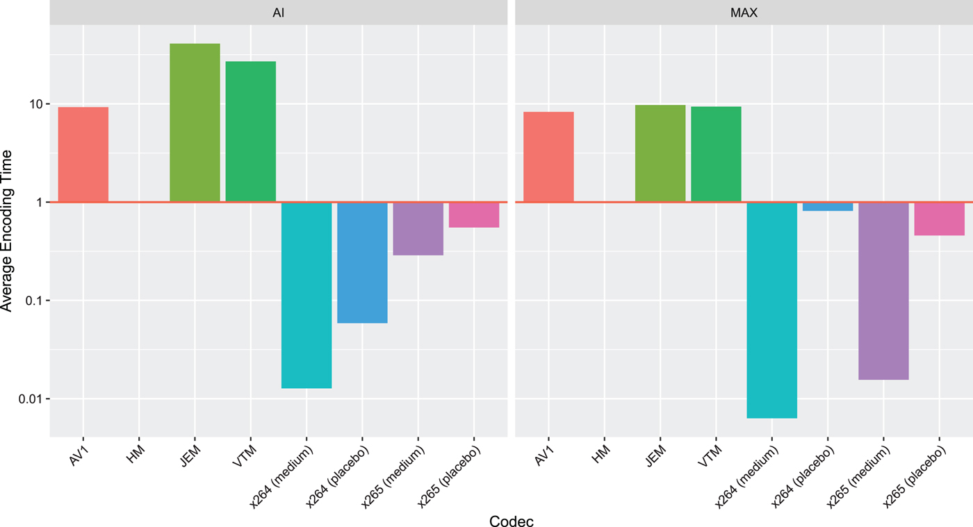
The results for the encoders are listed in Table 4 and visualized in Fig. 3. Due to the large spread of encoding time ratios (four orders of magnitude), the vertical axis has a logarithmic scale. Depending on the configuration and test sequence, either the JEM or the AV1 encoders are the slowest. It is without surprise that the x264 (medium) encoder is the fastest.
Table 4. Encoding time ratios for the two configurations AI (all-intra prediction) and MAX (most efficient motion compensation configuration for each codec) relative to the encoding time of HM. Values over 1 indicate slower encoders compared to HM, ratios below 1 faster encoders.


Fig. 3. Encoding time ratios for the two configurations AI (all-intra prediction) and MAX (most efficient motion compensation configuration for each codec) relative to the encoding time of HM. Values over 1 indicate slower encoders compared to HM, ratios below 1 faster encoders.
Although it is common practice in academic and standardization contributions to compare the complexity with relative numbers, we believe that this complicates the perception of how complex modern video codecs are. To facilitate the assessment of the encoding times, we exemplarily list the absolute encoding times for the 4k sequence Toddler Fountain in Table 5. It is observed that encoding one picture with x264 in the medium preset just takes a few seconds. At the other end of the scale, modern codecs such as JEM, VTM, or AV1 require more than half an hour or even more of computation per picture. Hence, it can be concluded that even in highly multi-threaded set-ups real-time encoding with these codecs configured for maximum coding efficiency is unfeasible.
Table 5. Absolute per picture encoding times for the sequence 4k Toddler Fountain. Times are given in the format hh:mm:ss. It is observed that the encoding times vary between few seconds per picture and more than one hour per picture.

For AV1, the trade-off between coding efficiency and encoding complexity can be tuned using the cpu-used parameter. This parameter was set to 0 for all of the presented experiments. With this value, the encoder is tuned for the highest coding efficiency but also for the highest encoding complexity. To further study the impact of the cpu-used parameter, we conducted a comparison of AV1 with cpu-used=0 versus AV1 withcpu-used=1. We observed that by using cpu-used=1, the coding efficiency drops by 2.4% (BD-Rate) averaged over our test set while the encoding speed is roughly 2.5 times faster.
The results for the decoders are listed in Table 6. Some interesting observations can be made for the decoder side: JEM shifts a certain amount of complexity to the decoder, e.g. with the decoder-side motion refinement. This is the reason why the decoder run time ratio of JEM is very high, $8\times$ for MAX compared to HM. The decoding complexity of AV1 is similar to the HM decoding complexity for high-resolution sequences and slightly lower for low-resolution sequences. It should be considered that some extend of software optimization was performed by the AV1 developers which was not performed by the HM developers. x264 and x265 do not include decoder implementations. Hence, they are omitted in the table.
Table 6. Decoding time ratios for the two configurations AI (all-intra prediction) and MAX (most efficient motion compensation configuration for each codec) relative to the decoding time of HM. Values over 1 indicate slower decoders compared to HM, ratios below 1 faster decoders.

In the end, video coding is a trade-off between coding efficiency and complexity. To assess how the codecs under review perform for this trade-off, we plot the BD-Rates of the codecs (relative to HM) over the encoding time ratio (relative to HM as well) in Fig. 4. A least-squares regression for a linear function was performed on the data. The resulting function is plotted along with 95% confidence intervals. For the all-intra configuration, a linear trend is observed. Considering the logarithmic horizontal axis it can be concluded that increasing the coding efficiency linearly results in exponentially increasing complexity of the coding tools. Although a similar trend is visible in the MAX data as well, the confidence intervals are too large to draw solid conclusions. The model fit by the regression is typically judged by the coefficient of determination ($R^2$ ). The range for $R^2$
 is between 0 and 1, where 1 indicates that the model fits the data perfectly and 0 that the model does not fit the data at all. The values for the two configurations are: $R^2_{{\rm AI}} = 0.97$
 and $R^2_{{\rm MAX}} = 0.75$
 .
.

Fig. 4. Trade-off of coding efficiency and encoder complexity (both relative to HM). A linear regression function is plotted with 95% confidence intervals. The coefficients of determination for the regression are $R^2_{{\rm AI}} = 0.97$ and $R^2_{{\rm MAX}} = 0.75$
 .
.
In real-world applications, often commercial encoders are used. The reason is that the complexity of reference implementations is too high to allow a deployment in products. For these encoders, the trade-off between coding efficiency and complexity can be configured depending on the requirements of the particular applications and systems. To perform such trade-offs with the reference implementations which we use for our comparison is not possible. However, it is known from the literature that by using commercial encoder products the HEVC encoding process can be sped-up by a factor of 30 with around 1% BD-Rate loss and by a factor of 300 for a BD-Rate loss of 12% compared to HM [Reference Grois, Nguyen and Marpe66].
VII. CONCLUSION
In this paper, we compared the video codecs AV1 (version 1.0.0-2242 from August 2019), HM, JEM, VTM (version 4.0 from February 2019), x264, and x265 under two different configurations: All Intra for the assessment of intra coding (which is also applicable to still image coding) and Maximum Coding Efficiency with all codec being tuned for their best coding efficiency settings. VTM achieves the highest coding efficiency in both configurations, followed by JEM and AV1. The worst coding efficiency is achieved by x264 and x265, even in the placebo preset for highest coding efficiency. AV1 gained a lot in terms of coding efficiency compared to previous versions and now outperforms HM by 24% BD-Rate gains. VTM gains 5% on average over AV1 in terms of BD-Rates. For 4K Sequences, AV1 is farther behind VVC with 20% loss. For the screen content sequences in the test set and some low resolutions, AV1 is even able to outperform VVC.
Thorsten Laude studied electrical engineering at the Leibniz University Hannover with a specialization in communication engineering and received his Dipl.-Ing. degree in 2013. In his diploma thesis, he developed a motion blur compensation algorithm for the scalable extension of HEVC. He joined InterDigital for an internship in 2013. At InterDigital, he intensified his research for HEVC. After graduating, he joined the Institut für Informationsverarbeitung at the Leibniz University Hannover where he is currently pursuing the Ph.D. degree. He contributed to several standardization meetings for HEVC and its extensions. His current research interests are intra coding for HEVC, still image coding, and machine learning for inter prediction, intra prediction, and encoder control.
Yeremia Gunawan Adhisantoso studied electrical engineering at the Leibniz University Hannover with specialization on computer engineering. He received his Master's degree in 2019 with his thesis on “Auto-encoder for Domain Adopted Head Pose Estimation”. He has been working on various research topics in the field of electrical engineering with interest in reachability analysis, deep learning, and genome coding.
Jan Voges studied electrical engineering at the Leibniz University Hannover with specialization on communications engineering. He received his Dipl.-Ing. degree from Leibniz University Hannover in 2015. After graduating, he joined the Institut für Informationsverarbeitung at the Leibniz University Hannover where he is currently working as a research assistant toward his Ph.D. degree. In the second half of the year 2018, he worked as a visiting scholar at the Carl R. Woese Institute for Genomic Biology at the University of Illinois at Urbana-Champaign. He is an active contributor to ISO/IEC JTC 1/SC 29/WG 11 (MPEG), where he contributes to the MPEG-G standard (ISO/IEC 23092) and where he serves as co-editor of parts 2 and 5 of MPEG-G. His current research ranges from information theory to bioinformatics.
Marco Munderloh achieved his Dipl.-Ing. degree in computer engineering with an emphasis on multimedia information and communication systems from the Technical University of Ilmenau, Germany, in 2004. His diploma thesis at the Fraunhofer Institute for Digital Media Technology dealt with holographic sound reproduction, the so-called wave field synthesis (WFS) where he helds a patent. During his work at the Fraunhofer Institute, he was involved in the development of the first WFS-enabled movie theater. At the Institut für Informationsverarbeitung of the Leibniz University Hannover, Marco Munderloh wrote his thesis with a focus on motion detection in scenes with non-static cameras for aerial surveillance applications and received his Dr.-Ing. degree in 2015.
Jörn Ostermann studied electrical engineering and communications engineering at the University of Hannover and Imperial College London. He received the Dipl.-Ing. and Dr.-Ing. degrees from the University of Hannover in 1988 and 1994, respectively. In 1994, he joined AT&T Bell Labs. From 1996 to 2003, he was with AT&T Labs – Research. Since 2003, he is a Full Professor and Head of the Institut für Informationsverarbeitung at Leibniz University Hannover, Germany. Since 2008, Jörn Ostermann is the Chair of the Requirements Group of MPEG (ISO/IEC JTC1 SC29 WG11). Jörn Ostermann received several international awards and is a Fellow of the IEEE. He published more than 100 research papers and book chapters. He is a coauthor of a graduate-level text book on video communications. He holds more than 30 patents. His current research interests are video coding and streaming, computer vision, 3D modeling, face animation, and computer–human interfaces.


 Open access