


Cobb (Reference Cobb1913) identifies three ways of defining the sex ratio: at conception, at time of birth and at age of reproduction. He notes that in England the second of these is about 0.509 and that there are more women than men at reproductive age. Pollard (Reference Pollard1969, p. 125) comments that the first of these, the ‘primary’, is very difficult to estimate and that little is known about it.
Figure 1 displays the sex ratio recorded for the Australian population during the period 1902−1965. It shows that there is a persistent tendency for the number of newborn males to exceed the number of females, giving support to the notion that natural selection influences the human sex ratio.

Fig. 1. The sex ratio at birth in the Australian population for the years 1902−65, derived from the table compiled by G. N. Pollard (Reference Pollard1969).
Vigor and Yule (Reference Vigor and Yule1906) studied the variation in sex ratio of 632 registration districts in England and Wales for the period 1881−1890. They compiled a two-way table with number of births on one axis and sex ratio interval on the other. They show that number of births and sex ratio (proportion of male newborns b) are not correlated but clearly dependent. Plotting the means of birth count by sex ratio interval they exhibit a bell shaped curve of frequency with mode just below b = 0.51, but some districts with small counts having b < 0.5 and some clearly above 0.53. The results are typical of those reported in countries with reliable birth registries.
Fisher (Reference Fisher1958), using part of Geissler’s data on sex ratio in families, found evidence of a tendency on the part of some parents to produce males or females. However, Lancaster (Reference Lancaster1950) concluded that the data were unreliable.
Cavalli-Sforza and Bodmer (Reference Cavalli-Sforza and Bodmer1971) contains a section on the sex ratio (pp. 650−666) and another on natural selection and the sex ratio (pp. 666−670). They identify reasons why the sex ratio could deviate from the expected 1:1. These include meiotic drive, gametic selection and differential mortality after fertilization.
Otto (Reference Otto2021) gives several models dealing with sex ratio determination in mammalians, in the course of which he cites many of the main contributors to the theory, but omits Karlin and Lessard (Reference Karlin and Lessard1986), which is a comprehensive survey of the field up to the time of publication. Otto’s second model explores the fate of a mutant that acts according to the combined number of mutants in the parental pair. Like most models in the literature it is deterministic.
Shaw and Mohler (Reference Shaw and Mohler1953) give a deterministic model of selection for sex ratio that derives change over three generations. They conclude: ‘Whenever the primary sex ratio of a population is not 0.5, selection favours sex ratio genes whose increase in frequency will cause a shift closer to 0.5. When the population sex ratio is already 0.5 there is no selection for sex ratio genes no matter what the direction or magnitude of their effects’ (p. 341). The experience of human populations contradicts this conclusion.
Karlin and Lessard (Reference Karlin and Lessard1986) give a brief comment on the Shaw-Mohler model (pp. 18−19). They note: ‘A proper stochastic diploid population genetic model of sex ratio variation needs to be investigated’ (p. 290). The model given here is a step in that direction.
Hofbauer and Sigmund (Reference Hofbauer and Sigmund1988, pp. 118−119) summarize the Shaw-Mohler model. In their afterword they note: ‘Evolution is an interplay of “chance and necessity”, but we have almost totally neglected stochastic methods.’
Fisher (Reference Fisher1930/1958, p. 145) concludes the chapter entitled ‘Sexual Reproduction and Sexual Selection’ with the comment: ‘It is shown that the action of Natural Selection will tend to equalize the parental expenditure devoted to the production of the two sexes; at the same time an understanding of the situations created by territory will probably reveal more than one way in which sexual preference gives an effective advantage in reproduction.’ In the same chapter there is a short section on ‘Natural Selection and the sex ratio’, which contains a remark of Darwin (Reference Darwin1871/1981) who admits that the sex ratio presents an ‘intricate problem’ (pp. 141−143). Fisher gives a verbal explanation of the sex ratio, directing the reader to his concept of ‘reproductive value’. His suggestions agree with the findings of Cobb (Reference Cobb1913) noted above. The model of Shaw and Mohler (Reference Shaw and Mohler1953) may be seen as a development of Fisher’s explanation.
However, Edwards (Reference Edwards2000) pointed out that Fisher’s (1930/1958) verbal discussion of sex ratio evolution probably followed Fisher’s knowledge of Düsing’s (1884, as cited in Edwards, Reference Edwards2000) analysis. Fisher (Reference Fisher1930/1958) may have assumed that experts in the field were familiar with Düsing’s model. In this sense, Düsing anticipated Shaw and Mohler (Reference Shaw and Mohler1953). Charnov (Reference Charnov1993, p. 24) gives credit to Fisher (1930) for the attention paid to sex ratio as a phenotypic trait, but intensive research came 35 years later. A full account of these issues is in Sections 1.5 and 1.6 of Seger and Stubblefield (Reference Seger, Stubblefield and Hardy2002).
The model given here makes no assumption about how natural selection determines the sex ratio, but males and females contribute equally to conception and sex (gender) is determined by which of two gametes is provided by the male. It permits conception to depart from 1:1 ratio of males to females. The model is stochastic, using Markov chain theory, in contrast to most of those constructed to study the sex ratio, which are deterministic. It starts from a formulation set out by Iosifescu (Reference Iosifescu1980), among others. It uses an idea introduced by Moran (Reference Moran1958) for potential change in a population when a single individual drops out. The stationary state of the Markov chain reveals the variance of the sex ratio, which is of use for interpreting the variation in sex ratio for small populations.
Markov chain model
Variations in the sex ratio are studied by assuming that the population has a constant number N of individuals and that the states are defined by the number of males 1, 2, …, (N-1) so that at any time there is at least one individual of each sex. An individual is selected at random for reproduction and death at each unit of time and is replaced by one individual. The probability that the offspring is male is p, the probability that the offspring is female is 1 – p. (Chromosome Y is transmitted from the male with probability p, X with probability 1 – p.)
If only one male is left at a reproduction-death event, a female is selected to reproduce and die, so p 11 = 1-p, is the probability that the offspring is female, and the number of males stays at 1. If the offspring is male, the number of males increases by 1 (to 2). The probability of this is p 12 = p. If only one female is left at a reproduction-death event, a male is chosen to reproduce and die. The number of males then stays the same (at N-1) with probability p N-1,N- 1 = p or decreases by 1 (to N-2) with probability p N-1,N-2 = 1-p.
The transition matrix, exemplified in Figure 2, and adapted to suit the model, has the following properties: the states range from 1 to N – 1 and refer to the number of males in the population:
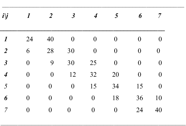
Fig. 2. Transition matrix related to sex ratio for population with N = 8 individuals and p = 5/8 (elements to be divided by 64).
for i to i – 1: q i = i(1 – p)/N. For i to i + 1: p i = (N- i)p/N. These for i = 2, …, N - 2. At the ‘ends’ r 1 = 1 – p, p 1 = p, r {N – 1} = p, q {N – 1} = 1 - p.
If the number of males at reproduction-death event is i, a male is chosen to die with probability i/N and a female with probability (N – i)/N. Combined with the transmission of chromosome X or Y as described, this gives the transition probabilities above.
The non-zero elements in the first and last rows are explained by the need to have at least one of each sex alive at all times. The stationary/limiting distribution $\{ \pi (i)\} $
is given by:
$\{ \pi (i)\} $
is given by:
 $$\begin{align*}x(N,p)\pi (1) = {B_1}(N,p);\;x(N,p)\pi (j) = \frac{N}{{N - 1}}{B_j}(N,p),j \\
= 2,...,N - 2;x(N,p)\pi (N - 1) = {B_{N - 1}}(N,p) \\ \end{align*}$$
$$\begin{align*}x(N,p)\pi (1) = {B_1}(N,p);\;x(N,p)\pi (j) = \frac{N}{{N - 1}}{B_j}(N,p),j \\
= 2,...,N - 2;x(N,p)\pi (N - 1) = {B_{N - 1}}(N,p) \\ \end{align*}$$
where ${B_j}(N, p) = \left( {_j^N} \right){p^j}{(1 - p)^{N - j}}, j = 1, 2, \ldots N - 2, N - 1{.}$
The norming constant is given by
 $$x(N,p) = {B_1}(N,p) + \frac{N}{{N - 1}}\sum\limits_{j = 2}^{j = N - 2} {{B_j}(N,p)} + {B_{N - 1}}(N,p).$$
The derivation is given in our Appendix below.
The case p = 1/2 reduces to : q i = i/(2N), i = 2 …, (N − 2); p i = (N − i)/(2N), i= 2,… (N −2); all other elements are zero.
The relevant truncated binomial distribution is then conveniently expressed using a normalizing constant $K(N) = \{ {2^N} - 4\} /\{ N - 1\} $
, giving terms
$K(N) = \{ {2^N} - 4\} /\{ N - 1\} $
, giving terms $K(N)\pi (i) = 1$
, when
$K(N)\pi (i) = 1$
, when $i = 1, N - 1;$
 $$ = \left( {_i^N} \right)/\{ N - 1\} , $$
when
$$ = \left( {_i^N} \right)/\{ N - 1\} , $$
when
 $$i = 2, \ldots , (N - 2)$$
.
$$i = 2, \ldots , (N - 2)$$
.
The transition matrix when N = 8 and p = 5/8 is given in Figure 2. The stationary state probabilities when N = 8 and p = ½ are $\pi = (1, 4, 8, 10, 8, 4, 1)/36$
, for states 1, 2, …, 7.
$\pi = (1, 4, 8, 10, 8, 4, 1)/36$
, for states 1, 2, …, 7.
The stationary state is a truncated and weighted binomial distribution (lacking state zero and state N) with number of ‘trials’ N and probability of ‘success’ p. An indication of the effect on the stationary distribution of varying p from ½ to 0.525 is a shift of the modal probability from 18 to 19.
The stationary distribution for the case N = 36 and p = 0.525 is displayed in Figure 3, to show visually the nature of the resulting asymmetry in moving from p = ½, and to make the important point that, even in a population with few members, the range of the number of males is concentrated about the expected number, that is that extreme numbers rarely occur.

Fig. 3. Stationary distribution for N = 36 and p = .525.
The outcome of a simulation of the model for N = 36 and p = .525 is displayed in Figure 4.

Fig. 4. Simulation of changes in male counts for case N = 36 and p = .525.
Acknowledgment
We thank a reviewer for critical comments and supplying details of early important studies of sex ratio. We have used a sentence or two of the referee’s own words. We also thank Paulo Otto for drawing our attention to his work.
Conflict of interest
none
Appendix A
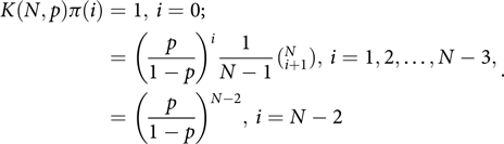
Iosifescu (Reference Iosifescu1980, pp. 67−68, p. 129) considers a Markov chain with transition matrix given in Figure A1. This describes a physical model of random walk type, which incorporates as a special case the celebrated Ehrenfest model for exchange of heat between isolated bodies, which addresses reversibility in statistical mechanics. We adapt a variation and generalization of the Ehrenfest model to explore variation over time of the sex ratio. The stationary state probability distribution $\{ \pi (i)\} $
in the general model given by Figure A1 is calculated from
$\{ \pi (i)\} $
in the general model given by Figure A1 is calculated from
 $$\pi (0) = \frac{1}{{1 + \sum\limits_{i = 1}^l {({p_0}...{p_{i - 1}})/({q_1}...{q_i})},}}$$
 $$\pi (i) = \frac{{({p_0}...{p_{i - 1}})/({q_1}...{q_i})}}{{1 + \sum\limits_{i = 1}^l {({p_0}...{p_{i - 1}})/({q_1}...{q_i})} }}.$$
Stationary Distribution 1
Markov chain with state space {1, 2,…, N – 1} (for the number of males present at a reproductive event). For i = 2,…., N – 2:
i → i + 1 with probability
 $${p_i} = \left( {{{N - i} \over N}} \right)p, $$
i → i – 1 with probability
 $${q_i} = {{i(1 - p)} \over N}, $$
and p 11 = 1 – p, p 12 = p, p N-1,N-1 = p, p N-1,N-2 = 1 - p. The r i ’s are not needed for the calculation of the limiting/stationary distribution.
Stationary Distribution 2. Iosifescu form
Change states from 1,2…N – 1 to 0,1,…, N – 2, so l = N – 2. Then p 0 = p, q N-2 = 1 – p, while
 $${p_i} = p\left( {1 - \frac{{i + 1}}{N}} \right) = \frac{p}{N}(N - i - 1),i = 1,2,...,N - 3,$$
 $${q_i} = (1 - p)\left( {\frac{{i + 1}}{N}} \right),i = 1,2,...,N - 3.$$
Then, using (2), with its denominator labelled as K(N,p), we have K(N,p)π(0) = 1, K(N,p)π(1) =
 $${{{p_0}} \over {{q_1}}} = {{pN} \over {(1 - p)2}}, $$
while for i > 1
$${{{p_0}} \over {{q_1}}} = {{pN} \over {(1 - p)2}}, $$
while for i > 1
 $$K\left( {N,p} \right)\pi \left( i \right) = \frac{{{p_0}...{p_{i - 1}}}}{{{q_1}...{q_i}}},$$
 \[ = \frac{{{p_0}}}{{{q_1}}}\;\frac{{p(N - 2)/N...p(N - i)/N}}{{(1 - p)3/N...(1 - p)(i + 1)/N}}\]
 \[ = {\left( {\frac{p}{{1 - p}}} \right)^i}\frac{{N(N - 2)(N - 3)...(N - i)}}{{2...(i + 1)}}\]
 $$= {\left( {\frac{p}{{1 - p}}} \right)^i}\frac{{N(N - 1)(N - 2)(N - 3)...(N - i)}}{{(N - 1)2...(i + 1)}}$$
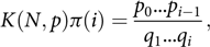
Thus
 $$\begin{align*}K(N,p)\pi (i) = 1,{\mkern 1mu} i = 0; \cr &\!\!\!\!\!\!\!\!\!\!\!\!\!\!\!\!\!\!\!\!\!\!\!\!\!\!\! = {\left( {\frac{p}{{1 - p}}} \right)^i}\frac{1}{{N - 1}}(_{i + 1}^N),{\mkern 1mu} i = 1,2, \ldots ,N - 3, \cr &\!\!\!\!\!\!\!\!\!\!\!\!\!\!\!\!\!\!\!\!\!\!\!\!\!\!\! = {\left( {\frac{p}{{1 - p}}} \right)^{N - 2}},{\mkern 1mu} i = N - 2.\end{align*}$$
Stationary Distribution 3
Returning to state space {1,2,…, N – 1}, put j = i + 1 in π(i), i = 0,1,…, N – 2 above to get
π*(j) = π(j – 1), j = 1,2,…, N – 1, so that
K(N,p)π*(j) = 1, j = 1;
 $$= {\left( {\frac{p}{{1 - p}}} \right)^{j - 1}}\frac{1}{{N - 1}}{{ (_{j}^N)}},j = 2,...,N - 2,$$
 $$= {\left( {\frac{p}{{1 - p}}} \right)^{N - 2}},j = N - 1.$$
Notice that for j = 2,…, N – 2 we may write
 $$\frac{1}{{(N - 1)p{{(1 - p)}^{N - 1}}}}(_j^N){p^j}{(1 - p)^{N - j}},j = 2,...,N - 2,$$
so the distribution may be regarded as a truncated and rescaled Binomial. This may be expressed more clearly, as follows.
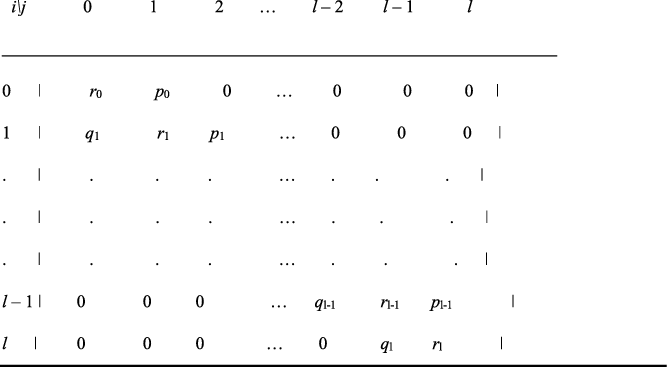
Fig. A1. Markov chain transition matrix constructed by Iosifescu (1968, p. 68).
Stationary Distribution 4,
Put $x(N, p) = Np{(1 - p)^{N - 1}}K(N, p)$
.
$x(N, p) = Np{(1 - p)^{N - 1}}K(N, p)$
.
Then $\{ \pi (i)\}, i = 1, 2, \ldots , N - 2, N - 1$
is given by
$\{ \pi (i)\}, i = 1, 2, \ldots , N - 2, N - 1$
is given by
 $$x(N,p)\pi (1) = {B_1}(N,p);x(N,p)\pi (j) = \frac{N}{{N - 1}}{B_j}(N,p),$$
 $$j = 2,...,N - 2;x(N,p)\pi (N - 1) = {B_{N - 1}}(N,p)$$
where
 $${B_j}(N,p) = {\text{ }}(_j^N){p^j}{(1 - p)^{N - j}},j = 1,2, \ldots ,N - 2,N - 1.$$
Consequently
$${B_j}(N,p) = {\text{ }}(_j^N){p^j}{(1 - p)^{N - j}},j = 1,2, \ldots ,N - 2,N - 1.$$
Consequently
 $$x(N,p) = {B_1}(N,p) + \frac{N}{{N - 1}}\sum\limits_{j = 2}^{j = N - 2} {{B_j}(N,p)} + {B_{N - 1}}(N,p).$$


 Open access