


1. Introduction
The area of complex networks concerns designing and analyzing structures that model well large real-life systems. It was empirically recognized that the common ground of such structures are small diameter, high clustering coefficient, heavy tailed degree distribution, and visible community structure (Bollobás & Riordan, Reference Bollobás and Riordan2003). Surprisingly, all those characteristics appear, no matter whether we investigate biological, social, or technological systems. An important growth of research in this field has been observed roughly since 1999 when Barabási and Albert introduced probably the most studied preferential attachment graph nowadays (Barabási & Albert, Reference Barabási and Albert1999). Their model is based on two mechanisms: growth (the graph is growing over time, gaining a new vertex and a bunch of edges at each time step) and preferential attachment (an arriving vertex is more likely to attach to the other vertices with a high degree rather than with a low degree). It captures two out of four universal properties of the real networks, which are a heavy tailed degree distribution and a small world phenomenon.
A number of theoretical complex networks models were presented since then. For the interesting extensions of the Barabási-Albert model, one may check, for example, by Dorogovtsev et al. (Reference Dorogovtsev, Mendes and Samukhin2000), where preferential attachment rule includes also, so-called, initial attractiveness of each vertex, by Cooper & Frieze (Reference Cooper and Frieze2003) where insertion of edges between existing vertices is allowed, or spatial preferential attachment (SPA) model (Aiello et al., Reference Aiello, Bonato, Cooper, Janssen and Prałat2008, Jacob & Mörters, Reference Jacob and Mörters2015, Kaiser & Hilgetagr, Reference Kaiser and Hilgetagr2004) in which vertices are given a spatial position and preferential attachment rule favors short connections. A noticeable disadvantage of many preferential attachment models meant to reflect real-life networks is the lack of a visible community structure, that is, low modularity.
Modularity is a parameter measuring how clearly a network may be divided into communities. It was introduced by Newman and Girvan in Newman & Girvan (Reference Newman and Girvan2004). A graph has high modularity if it is possible to partition the set of its vertices into communities inside which the density of edges is remarkably higher than the density of edges between different communities (we give its precise definition in the next section). Modularity is known to have some drawbacks (for a thorough discussion check (Lancichinetti & Fortunato, Reference Lancichinetti and Fortunato2011)). Nevertheless, today it remains a popular measure, and it is widely used in most common algorithms for community detection [Blondel et al., Reference Blondel, Guillaume, Lambiotte and Lefebvre2008, Fortunato & Hric Reference Fortunato and Hric2016, Traag et al., Reference Traag, Waltman and van Eck2019). Most of the up-to-date results on the modularity for various classes of graphs are summarized in the appendix of McDiarmid & Skerman (Reference McDiarmid and Skerman2020) . One finds there, among others, the results for random  $d$-regular graphs (McDiarmid & Skerman, Reference McDiarmid and Skerman2018; Prokhorenkova et al., Reference Prokhorenkova, Pralat and Raigorodskii2017), random planar graphs (McDiarmid & Skerman, Reference McDiarmid and Skerman2018), treelike graphs (McDiarmid & Skerman, Reference McDiarmid and Skerman2018) (graphs with low treewidth), Erdős-Rényi graphs (McDiarmid & Skerman, Reference McDiarmid and Skerman2020), and preferential attachment graphs. The latter ones were studied by Prokhorenkova et al. (Reference Prokhorenkova, Prałat and Raigorodskii2016) and (Reference Prokhorenkova, Pralat and Raigorodskii2017) in the context of the Barabási-Albert model. For very recent results on the modularity for random graphs (
 $3$-regular ones, the ones with a given degree sequence and the ones on the hyperbolic plane) consult (Chellig et al., Reference Chellig, Fountoulakis and Skerman2021; Chellig et al., Reference Chellig, Fountoulakis and Skerman2022). Also, for a new result on the modularity of minor-free graphs one may check (Lasoń & Sulkowska, Reference Lasoń and Sulkowska2022).
It is well known that the real-life social or biological networks are highly modular (Fortunato, Reference Fortunato2010; Girvan & Newman Reference Girvan and Newman2002). On the other hand, just several power-law models featuring existence of communities were introduced so far. One may check LFR (Lancichinetti et al., Reference Lancichinetti, Fortunato and Radicchi2008) and ABCD (Kamiński et al., Reference Kamiński, Prałat and Théberge2021) benchmarks as one of the few examples. In these models, not only the degrees but also the sizes of communities follow a power-law. Some asymptotic results for the modularity of ABCD were given recently in Kamiński et al. (Reference Kamiński, Prałat and Théberge2022). Both LFR and ABCD are, however, static graphs (the number of nodes must be given in advance at the generation phase). Good modularity properties are obtained also by geometric models, like already mentioned SPA graphs (Aiello et al., Reference Aiello, Bonato, Cooper, Janssen and Prałat2008; Jacob & Mörters, Reference Jacob and Mörters2015; Kaiser & Hilgetagr, Reference Kaiser and Hilgetagr2004) (for the modularity analysis of SPA model presented in Aiello et al. (Reference Aiello, Bonato, Cooper, Janssen and Prałat2008) one may check (Prokhorenkova et al., Reference Prokhorenkova, Prałat and Raigorodskii2016)). However, they additionally use a spatial metric. An interesting proposition appears also in papers by Avin et al. (Reference Avin, Daltrophe, Keller, Lotker, Mathieu, Peleg and Pignolet2020) and (Reference Avin, Keller, Lotker, Mathieu, Peleg and Pignolet2015), where a preferential attachment model featuring two types of vertices, reflecting minority and majority in the society (thus connect to others from the same social group) or heterophily (when individuals prefer to join a different group). We present it in more details in the light of our results in Section 6.
Note that almost all the up-to-date complex networks models are graph models; thus, they mirror only binary relations. In practical applications,  $k$-ary relations (co-authorship, groups of interests, protein reactions) are often modeled in graphs by cliques which may lead to a profound information loss.
1.1. Results
Within this article, we propose a dynamic model with high modularity by preserving a heavy tailed degree distribution and not using a spatial metric. Moreover, our model is a random hypergraph (not a graph), thus, it can reflect  $k$-ary relations. A first preferential attachment hypergraph model was introduced by Wang et al. (Reference Wang, Rong, Deng and Zhang2010). However, it was restricted just to a specific subfamily of uniform acyclic hypergraphs (the analogue of trees within graphs). The first rigorously studied non-uniform hypergraph preferential attachment model was proposed only in 2019 by Avin et al. (Reference Avin, Lotker, Nahum and Peleg2019). Its degree distribution follows a power-law. However, our empirical results indicate that this model has a weakness of low modularity (see Section 7). To the best of our knowledge, the model proposed within this article is the first dynamic non-uniform hypergraph model with degree sequence following a power-law and exhibiting clear community structure. We experimentally show that the features of our model correspond to the ones of a real co-authorship network built upon Scopus database.
1.2. Paper organization
Basic definitions are introduced in Section 2. In Section 3, we present a universal preferential attachment hypergraph model which unifies many existing models (from classical Barabási-Albert graph (Barabási & Albert, Reference Barabási and Albert1999) to Avin et al., preferential attachment hypergraph (Avin et al., Reference Avin, Lotker, Nahum and Peleg2019)). In Section 4, we use it as a component in a stochastic block model to build a general hypergraph with good modularity properties. Theoretical bounds for its modularity one finds in Section 5. In Section 6, we compare our model with minority-majority graphs introduced in Avin et al. (Reference Avin, Daltrophe, Keller, Lotker, Mathieu, Peleg and Pignolet2020), (Reference Avin, Keller, Lotker, Mathieu, Peleg and Pignolet2015), and experimental results on a real data are presented in Section 7. Further works are discussed in Section 8. The Appendix contains several technical proofs.
2. Basic definitions and notation
We define a hypergraph  $H$ as a pair
  $H=(V,E)$, where
  $V$ is a set of vertices and
  $E$ is a multiset of hyperedges, that is, non-empty, unordered multisets of
  $V$. We allow for a multiple appearance of a vertex in a hyperedge (self-loops) as well as a multiple appearance of a hyperedge in
  $E$. The degree of a vertex
  $v$ in a hyperedge
  $e$, denoted by
  $d(v,e)$, is the number of times
  $v$ appears in
  $e$. The cardinality of a hyperedge
  $e$ is
  $|e| = \sum _{v \in e} d(v,e)$. The degree of a vertex
  $v \in V$ in
  $H$ is understood as the number of times it appears in all hyperedges, that is,
  $\deg (v) = \sum _{e \in E} d(v,e)$. If
  $|e|=k$ for all
  $e \in E$,
  $H$ is said to be
  $k$-uniform.
We consider hypergraphs that grow by adding vertices and/or hyperedges at discrete time steps  $t=0,1,2,\ldots$ according to some rules involving randomness. The random hypergraph obtained at time
  $t$ will be denoted by
  $H_t=(V_t,E_t)$ and the degree of
  $u \in V_t$ in
  $H_t$ by
  $\deg _t(u)$. By
  $D_t$, we denote the sum of degrees at time
  $t$, that is,
  $D_t = \sum _{u \in V_t} \deg _t(u)$.
 $N_{k,t}$ stands for the number of vertices in
  $H_t$ of degree
  $k$. We write
  $f(k) \sim g(k)$ if
  $f(k)/g(k) \xrightarrow{k \rightarrow \infty } 1$. We say that the degree distribution of a random hypergraph follows a power-law if the fraction of vertices of degree
  $k$ is proportional to
  $k^{-\beta }$ for some exponent
  $\beta \geq 1$. Formally, we will interpret it as
  $\lim _{t \rightarrow \infty }{\mathbb{E}}\left [\frac{N_{k,t}}{|V_t|}\right ] \sim c \cdot k^{-\beta }$ for some positive constant
  $c$ and
  $\beta \geq 1$. We say that an event
  $A$ occurs with high probability (whp) if the probability
  $\mathbb{P}[A]$ depends on a certain number
  $t$ and tends to
  $1$ as
  $t$ tends to infinity.
As the hypergraph gets large, the probability of creating a self-loop can be well bounded and is quite small provided that the sizes of hyperedges are reasonably bounded.
Introduced by Newman and Girvan, modularity measures the presence of community structure in the graph.
Definition 1 ([40]). Let  $G=(V,E)$ be a graph with at least one edge. For a partition
  $\mathcal{A}$ of vertices of
  $G$, we define its modularity score on
  $G$ as
 \begin{align*} q_{\mathcal{A}}(G) = \sum _{A \in \mathcal{A}} \left (\frac{|E(A)|}{|E|} - \left (\frac{vol(A)}{2|E|}\right )^2 \right ), \end{align*}
where  $E(A)$ is the set of edges within
  $A$ and
  $vol(A) = \sum _{v \in A} \deg (v)$ (
 $\deg (v)$ stands for the degree of
  $v$ in
  $G$). The modularity of
  $G$ is then given by
  $q^*(G) = \max _{\mathcal{A}} q_{\mathcal{A}}(G)$.
Conventionally, a graph with no edges has modularity equal to  $0$. The value
  $\sum _{A \in \mathcal{A}} \frac{|E(A)|}{|E|}$ is called an edge contribution while
  $\sum _{A \in \mathcal{A}} \left (\frac{vol(A)}{2|E|}\right )^2$ is a degree tax. A single summand of the modularity score is the difference between the fraction of edges within
  $A$ and the expected fraction of edges within
  $A$ if we considered a random multigraph on
  $V$ with the degree sequence given by
  $G$. The value of
  $q^*(G)$ always falls into the interval
  $[0,1)$.
Several approaches to define a modularity for hypergraphs can be found in contemporary literature. Some of them flatten a hypergraph to a graph (e.g. by replacing each hyperedge by a clique) and apply a modularity for graphs (see e.g. (Kumar et al., Reference Kumar, Vaidyanathan, Ananthapadmanabhan, Parthasarathy and Ravindran2020; Neubauer & Obermayer, Reference Neubauer and Obermayer2009)). Others are based on information entropy modularity (Yang et al., Reference Yang, Wang, Bhuiyan and Choo2017). We want to stick to the classical definition from Newman & Girvan (Reference Newman and Girvan2004) and preserve a rich hypergraph structure, thus we work with the definition proposed by Kamiński et al. (Reference Kamiński, Poulin, Prałat, Szufel and Théberge2019).
Definition 2 (Kamiński et al., Reference Kamiński, Poulin, Prałat, Szufel and Théberge2019). Let  $H=(V,E)$ be a hypergraph with at least one hyperedge. For
  $\ell \geq 1$, let
  $E_{\ell } \subseteq E$ denote the set of hyperedges of cardinality
  $\ell$. For a partition
  $\mathcal{A}$ of vertices of
  $H$, we define its modularity score on
  $H$ as
 \begin{align*} q_{\mathcal{A}}(H) = \sum _{A \in \mathcal{A}} \left (\frac{|E(A)|}{|E|} - \sum _{\ell \geq 1} \frac{|E_{\ell }|}{|E|} \cdot \left (\frac{vol(A)}{vol(V)}\right )^{\ell } \right ), \end{align*}
where  $E(A)$ is the set of hyperedges within
  $A$ (a hyperedge is within
  $A$ if all its vertices are contained in
  $A$),
$A$),  $vol(A) = \sum _{v \in A} deg(v)$ and
  $vol(V) = \sum _{v \in V} deg(v)$. The modularity of
  $H$ is then given by
  $q^*(H) = \max _{\mathcal{A}} q_{\mathcal{A}}(H)$.
A single summand of the degree tax is the expected number of hyperedges within  $A$ if we considered a random hypergraph on
  $V$ with the degree sequence given by
  $H$ and having the same number of hyperedges of corresponding cardinalities.
Remark 1. In the above definition, only the hyperedges that are all contained in a single community may increase the edge contribution. This is, so-called, strict variant of the hypergraph modularity. In the literature, one finds also the other variants, for example, majority in which the hyperedge increases the edge contribution if majority of its vertices belong to a single community. For a detailed discussion and other variants consult (Kamiński et al., Reference Kamiński, Poulin, Prałat, Szufel and Théberge2019; Kamiński et al., Reference Kamiński, Prałat and Théberge2021). First algorithms for community detection in hypergraphs based on those definitions one finds in Antelmi et al. (Reference Antelmi, Cordasco, Kamiński, Prałat, Scarano, Spagnuolo and Szufel2020); Kamiński et al. (Reference Kamiński, Poulin, Prałat, Szufel and Théberge2019); Kamiński et al. (Reference Kamiński, Prałat and Théberge2021).
Remark 2. It is worth mentioning that to model  $k$-ary relations, one may also turn to bipartite graphs with two kinds of nodes: one kind representing actors of the network and the other the groups to which actors may belong (e.g. scientists are actors and scientific articles constitute the groups). Then, the edge always connects two vertices of different kinds reflecting membership of an actor in a given group. Such representation is, in many respects, equivalent to the hypergraph one. For example, the degree distribution of the actors’ part coincide with the degree distribution obtained by modeling this network by a hypergraph (indeed, a degree of an actor is the number of groups, thus hyperedges, to which she belongs). Consult (Newman et al. (Reference Newman, Watts and Strogatz2002) for some explicit work on such bipartite structures and (Newman et al., Reference Newman, Strogatz and Watts2001) for machinery to investigate its properties. In Ghoshal et al. (Reference Ghoshal, Zlatić, Caldarelli and Newman2009), generalization to tripartite graph is presented. For random variants (called random intersection graphs), one may check the surveys (Bloznelis et al., Reference Bloznelis, Godehardt, Jaworski, Kurauskas and Rybarczyk2013a; Reference Bloznelis, Godehardt, Jaworski, Kurauskas and Rybarczyk2013b) and for some variants of bipartite graph generators the chapter (Penschuck et al., Reference Penschuck, Brandes, Hamann, Lamm, Meyer, Safro, Schulz and Bader2022).
3. General preferential attachment hypergraph model
In this section, we generalize a hypergraph model proposed by Avin et al. (Reference Avin, Lotker, Nahum and Peleg2019). The model from Avin et al. (Reference Avin, Lotker, Nahum and Peleg2019) allows for two different actions at a single time step—attaching a new vertex by a hyperedge to the existing structure or creating a new hyperedge on already existing vertices. We allow for four different events at a single time step, admit the possibility of adding more than one hyperedge at once, and draw the cardinality of newly created hyperedge from more than one distribution. The events allowed at a single time step in our model  $H_t$ are as follows: adding an isolated vertex, adding a vertex and attaching it to the existing structure by
  $m$ hyperedges, adding
  $m$ hyperedges, or doing nothing. The last event “doing nothing” is included since later we put
  $H_t$ in a broader context of a stochastic block model, where it serves as a single community. “Doing nothing” indicates a time slot in which nothing associated directly with
  $H_t$ happens but some event takes place in the other part of the whole stochastic block model (see Section 4).
3.1. Model  $\mathbf{H(H_0,p,Y,X,m,\gamma )}$
The general hypergraph model  $H$ is characterized by the six following parameters:
(1)
$H_0$—the initial hypergraph, seen at $t=0$;-
(2)
$\mathbf{p} = (p_v,p_{ve},p_e)$—the vector of probabilities indicating, what are the chances that a particular type of event occurs at a single time step; we assume $p_v + p_{ve} + p_e \in (0,1]$; additionally $p_e$ is split into the sum of $r$ probabilities $p_e = p_e^{(1)} + p_e^{(2)} + \ldots + p_e^{(r)}$ which allows for adding hyperedges whose cardinalities follow different distributions; -
(3)
$Y = (Y_0, Y_1, \ldots, Y_t, \ldots )$—independent random variables, giving the cardinalities of the hyperedges that are added together with a vertex at a single time step; -
(4)
$X = ((X_1^{(1)}, \ldots, X_t^{(1)}, \ldots ), \ldots, (X_1^{(r)}, \ldots, X_t^{(r)}, \ldots ))$ - $r$ sequences of independent random variables, representing the cardinalities of the hyperedges that are added at a single time step when no new vertex is added; -
(5)
$m$—the number of hyperedges added at once; -
(6)
$\gamma \geqslant 0$—a parameter appearing in the formula for the probability of choosing a particular vertex to a newly created hyperedge.


Here is how the structure of  $H = H(H_0,p,Y,X,m,\gamma )$ is being built. We start with some non-empty hypergraph
  $H_0$ at
  $t=0$. We assume for simplicity that
  $H_0$ consists of a hyperedge of cardinality
  $1$ over a single vertex. Nevertheless, all the proofs may be generalized to any fixed initial
  $H_0$. “Vertices chosen from
  $V_t$ in proportion to degrees” means that vertices are chosen independently (possibly with repetitions) and the probability that any
  $u$ from
  $V_t$ is chosen is
 \begin{align*} \mathbb{P}[u \text{ is chosen}] = \frac{\deg _t(u) + \gamma }{\sum _{v \in V_t}(\deg _t(v)+\gamma )} = \frac{\deg _t(u) + \gamma }{D_t + \gamma |V_t|}. \end{align*}
For  $t \geqslant 0$ we form
  $H_{t+1}$ from
  $H_t$ choosing only one of the following events according to
  $\mathbf{p}$.
• With probability
$p_v$: Add one new isolated vertex.-
• With probability
$p_{ve}$: Add one vertex $v$. Draw a value $y$ being a realization of $Y_t$. Then repeat $m$ times: select $y-1$ vertices from $V_{t}$ in proportion to degrees; add a new hyperedge consisting of $v$ and $y-1$ selected vertices. • With probability
$p_{e}^{(1)}$: Draw a value $x$ being a realization of $X_t^{(1)}$. Then repeat $m$ times: select $x$ vertices from $V_{t}$ in proportion to degrees; add a new hyperedge consisting of $x$ selected vertices.-
• With probability
$p_{e}^{(r)}$: Draw a value $x$ being a realization of $X_t^{(r)}$. Then repeat $m$ times: select $x$ vertices from $V_{t}$ in proportion to degrees; add a new hyperedge consisting of $x$ selected vertices. -
• With probability
$1-(p_v+p_{ve}+p_{e})$: Do nothing.


We allow for  $r$ different distributions from which one can draw the cardinality of newly created hyperedges. Later, when
  $H_t$ serves as a single community in the context of the whole stochastic block model, this trick allows for spanning a new hyperedge across several communities drawing vertices from each of them according to different distributions. This reflects some possible real-life applications. Think of an article authored by people from two different research centers. Our experimental observation is that it is very unlikely that the number of authors will be distributed uniformly among two centers. More often, one author represents one center, while the others are affiliated with the second one.
3.2. Degree distribution of $\mathbf{H(H_0,p,Y,X,m,\gamma )}$

In this section, we prove that the degree distribution of  $H = H(H_0,p,Y,X,m,\gamma )$ follows a power-law with
  $\beta \gt 2$. We assume that supports of random variables indicating cardinalities of hyperedges are bounded. This assumption is in accord with potential applications—think of co-authors, groups of interest, protein reactions, etc. Moreover, we assume that their expectations are constant. First, we state a technical lemma. For its proof consult Section A in the Appendix.
Lemma 1. If  $\lim _{t \rightarrow \infty } \frac{{\mathbb{E}}[N_{k,t}]}{t} \sim c k^{-\beta }$ for some positive constant
  $c$ then
 \begin{align*} \lim _{t \rightarrow \infty }{\mathbb{E}}\left [\frac{N_{k,t}}{|V_t|}\right ] \sim \frac{c}{p_v+p_{ve}} k^{-\beta }. \end{align*}
(Here “  $\sim$” refers to the limit by
  $k \rightarrow \infty$.)
Theorem 1. Consider a hypergraph  $H = H(H_0,\mathbf{p},Y,X,m,\gamma )$ for any
  $t\gt 0$. Let
  $i \in \{1,\ldots,r\}$. Let
  ${\mathbb{E}}[Y_t] = \mu _0$, and
  ${\mathbb{E}}[X_t^{(i)}] = \mu _i$. Moreover, let
  $1 \leqslant Y_t \lt t^{1/4}$ and
  $1 \leqslant X_t^{(i)} \lt t^{1/4}$. Then, the degree distribution of
  $H$ follows a power-law with
 \begin{equation*} \beta = 2+\frac {\gamma \bar {V} + m \cdot p_{ve}}{\bar {D} - m \cdot p_{ve}},\end{equation*}
where  $\bar{V} = p_v+p_{ve}$ and
  $\bar{D} = m(p_{ve}\mu _0 + p_e^{(1)}\mu _1 + \ldots + p_e^{(r)}\mu _r)$ which are the expected number of vertices added per single time step and the expected number of vertices that increase their degree in a single time step, respectively.
Sketch of proof. (For the full proof consult Section A in the Appendix.) We prove that  $\lim _{t \rightarrow \infty } \frac{{\mathbb{E}}[N_{k,t}]}{|V_t|} \sim \tilde{c} k^{-\beta }$ (determining the exact constant
  $\tilde{c}$). By Lemma 1 we know that it suffices to show that
  $\lim _{t \rightarrow \infty } \frac{{\mathbb{E}}[N_{k,t}]}{t} \sim c k^{-\beta }$ for some positive constant
  $c$. We take a standard master equation approach that can be found, for example, in Chung & Lu (Reference Chung and Lu2006) or Avin et al. (Reference Avin, Lotker, Nahum and Peleg2019). The initial hypergraph
  $H_0$ consists of a single hyperedge of cardinality
  $1$ over a single vertex thus
  $N_{0,0} = 0$ and
  $N_{1,0}=1$. Now, let
  ${\mathcal{F}}_t$ be the
  $\sigma$-algebra associated with the probability space at time
  $t$. Let
  $Q_{d,k,t}$ denote the probability that a specific vertex of degree
  $k$ was chosen
  $d$ times to be included in new hyperedges at time
  $t$. Moreover, let
  $Z_t$ be the random variable chosen at step
  $t$ among
  $Y_t, X_t^{(1)}, \ldots, X_t^{(r)}$ according to
  $(p_v,p_{ve},p_e^{(1)},\ldots,p_e^{(r)})$. For
  $t \geqslant 1$ we get that
 \begin{align*}{\mathbb{E}}[N_{0,t} |{\mathcal{F}}_{t-1}] = p_v + N_{0,t-1} Q_{0,0,t} \end{align*}
and when  $k \geqslant 1$
 \begin{align*}{\mathbb{E}}[N_{k,t} |{\mathcal{F}}_{t-1}] = \delta _{k,m} p_{ve} + \sum _{i=0}^{\min \{k,mZ_t\}} N_{k-i,t-1} Q_{i,k-i,t}, \end{align*}
where  $\delta _{k,m}$ is the Kronecker delta. The proof then follows from the tedious analysis of this recursive equation.
Remark 3. In the proof of Theorem 1, we show more than the statement tells. Not only we show that the degree distribution of  $H$ follows a power-law but also we determine the exact constant
  $\tilde{c}$ in the expression
  $\lim _{t \rightarrow \infty } \frac{{\mathbb{E}}[N_{k,t}]}{|V_t|} \sim \tilde{c} k^{-\beta }$, which is
  $\tilde{c} = \frac{c}{p_v+p_{ve}}$, where
  $c = p_v D\cdot \frac{\Gamma (\gamma +D)}{\Gamma (\gamma )} + p_{ve} D\cdot \frac{\Gamma (m+\gamma +D)}{\Gamma (m+\gamma )}$ and
  $D = \frac{\bar{D}+\gamma \bar{V}}{\bar{D}-m p_{ve}}$ (
 $\Gamma (x)$ stands for the gamma function).
Below we present a bunch of examples showing that our theorem generalizes the results for well known models.
Example 1 (Barabási-Albert graph model, (Barabási & Albert, Reference Barabási and Albert1999)). In a single time step, we always add one new vertex and attach it with  $m$ edges (in proportion to degrees) to existing structure. Thus
  $p_v = 0$,
  $p_{ve}=1$,
  $p_e=0$,
  $\bar{V}=1$,
  $Y_t=2$,
  $\bar{D}=2m$,
  $\gamma =0$ and we get
  $\beta = 2+\frac{m}{2m-m} = 3.$
Example 2 (Preferential attachment scheme with vertex- and edge-step, (Chung & Lu, Reference Chung and Lu2006), Chapter  $3$). In a single time step: we either (with probability
  $p$) add one new vertex and attach it with an edge (in proportion to degrees) to existing structure; otherwise, we just add an edge (in proportion to degrees) to existing structure. Thus
  $p_v = 0$,
  $p_{ve}=p$,
  $p_e=1-p$,
  $\bar{V}=p$,
  $Y_t=2$,
  $r=1$,
  $X_t^{(1)}=2$,
  $\bar{D}=2$,
  $m=1$,
  $\gamma =0$ and we get
  $\beta = 2+\frac{p}{2-p}$.
Example 3 (Avin et al., hypergraph model, (Avin et al., Reference Avin, Lotker, Nahum and Peleg2019)). In a single time step, we either (with probability  $p$) add one new vertex and attach it with a hyperedge of cardinality
  $Y_t$ (in proportion to degrees) to existing structure; otherwise, we just add a hyperedge of cardinality
  $Y_t$ to existing structure. The assumptions on
  $Y_t$ and the sum of degrees
  $D_t$ are as follows:
(1)
$\lim _{t \rightarrow \infty } \frac{{\mathbb{E}}[D_{t-1}]/t}{{\mathbb{E}}[Y_t]-p_{ve}} = D \in (0,\infty )$,-
(2)
${\mathbb{E}}[|\frac{1}{D_t}-\frac{1}{{\mathbb{E}}[D_t]}|] = o(1/t)$, -
(3)
${\mathbb{E}}\left [\frac{Y_t^2}{D_{t-1}^2}\right ] = o(1/t)$.
The result from Avin et al. (Reference Avin, Lotker, Nahum and Peleg2019) states that the degree distribution of the resulting hypergraph follows a power-law with  $\beta = 1 + D$. Note that in our model
  $\lim _{t \rightarrow \infty } \frac{{\mathbb{E}}[D_{t-1}]/t}{{\mathbb{E}}[Y_t]-p_{ve}} = \frac{\bar{D}}{\bar{D}-p_{ve}}$. Setting
  $p_v = 0$,
  $p_{ve}=p$,
  $p_e=1-p$,
  $\bar{V}=p$,
  $m=1$,
  $\gamma =0$ we get
  $\beta = 2+\frac{p_{ve}}{\bar{D}-p_{ve}} = 1 + \frac{\bar{D}}{\bar{D}-p_{ve}} = 1 + D$.
Remark 4. Even though our result from this section may seem similar to what was obtained by Avin et al., it is easy to indicate cases that are covered by our model but not by the one from Avin et al. (Reference Avin, Lotker, Nahum and Peleg2019) and vice versa. Indeed, the model from Avin et al. (Reference Avin, Lotker, Nahum and Peleg2019] admits a wide range of distributions for  $Y_t$. In particular, as authors underline, three mentioned assumptions hold for
  $Y_t$ which is polynomial in
  $t$. This is the case not covered by our model (we upper bound
  $Y_t$ by
  $t^{1/4}$) but we also cannot think of real-life examples that would require bigger hyperedges. However, we can think of some natural examples that break requirements from Avin et al. (Reference Avin, Lotker, Nahum and Peleg2019) but are admissible in our model. Put
  $Y_t = 2$ if
  $t$ is odd and
  $Y_t = 3$ if
  $t$ is even. Then,
 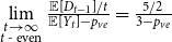 $\lim \limits _{\substack{t \rightarrow \infty \\ t \text{ - even}}} \frac{{\mathbb{E}}[D_{t-1}]/t}{{\mathbb{E}}[Y_t]-p_{ve}} = \frac{5/2}{3-p_{ve}}$ and
 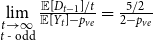 $\lim \limits _{\substack{t \rightarrow \infty \\ t \text{ - odd}}} \frac{{\mathbb{E}}[D_{t-1}]/t}{{\mathbb{E}}[Y_t]-p_{ve}} = \frac{5/2}{2-p_{ve}}$; thus, the limit
 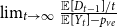 $\lim _{t \rightarrow \infty } \frac{{\mathbb{E}}[D_{t-1}]/t}{{\mathbb{E}}[Y_t]-p_{ve}}$ does not exist. Whereas in our model we are allowed to put
  $r=2$,
 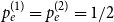 $p_e^{(1)}=p_e^{(2)}=1/2$,
  $X_t^{(1)} = 2$,
  $X_t^{(2)} = 3$ which probabilistically simulates stated example.
4. Hypergraph model with high modularity
In this section, we present a new preferential attachment hypergraph model which features partition into communities. We prove that its degree distribution follows a power-law. Its structure benefits from the stochastic block model for graphs (Holland et al., Reference Holland, Laskey and Leinhardt1983). In the stochastic block model, a vertex set is partitioned into disjoint communities  $C^{(1)},\ldots,C^{(r)}$ while the edge set is sampled according to a symmetric matrix
  $P_{r \times r}$ of probabilities: vertices
  $v \in C_i$ and
  $u \in C_j$ are connected with probability
  $P_{ij}$, independently of the others. (There exist other graph models with a built-in community structure, for example, LFR (Lancichinetti et al., Reference Lancichinetti, Fortunato and Radicchi2008) or ABCD (Kamiński et al., (Reference Kamiński, Prałat and Théberge2021) benchmarks; we chose a stochastic block model for its simplicity). To the best of our knowledge, no mathematical model so far consolidated preferential attachment, possibility of having hyperedges and clear community structure. We denote our hypergraph by
  $G_t=(V_t,E_t)$. At each time step, either a new vertex (vertex-step) or a new hyperedge (hyperedge-step) is added to the existing structure. The set of vertices of
  $G_t$ is partitioned into
  $r$ communities
  $V_t = C_t^{(1)} \mathbin{\dot{\cup }} C_t^{(2)} \mathbin{\dot{\cup }} \ldots \mathbin{\dot{\cup }} C_t^{(r)}$. Whenever a new vertex is added to
  $G_t$, it is assigned to just one out of
  $r$ communities and stays there forever.
4.1. Model $\mathbf{G(G_0,p,M,X,P,\gamma )}$

Hypergraph model  $G$ is characterized by six parameters:
(1)
$G_0$—initial hypergraph seen at time $t=0$ with vertices partitioned into $r$ communities $V_0 = C_{0}^{(1)} \mathbin{\dot{\cup }} C_{0}^{(2)} \mathbin{\dot{\cup }} \ldots \mathbin{\dot{\cup }} C_{0}^{(r)}$;-
(2)
$p \in (0,1)$—the probability of taking a vertex-step; -
(3) vector
$M=(m_1, m_2, \ldots, m_r)$ with all $m_i$ positive, constant and summing up to $1$; $m_i$ is the probability that a randomly chosen vertex belongs to $C_t^{(i)}$; -
(4)
$d$-dimensional matrix $P_{r \times \ldots \times r}$ of hyperedge probabilities ($P_{i_1,i_2,\ldots,i_d}$ is the probability that communities $i_1, \ldots, i_d$ share a hyperedge); $d$ is the upper bound for the number of distinct communities shared by a single hyperedge ($d \leq r$); -
(5)
$X = ((X_1^{(1)}, \ldots, X_t^{(1)},\ldots ), \ldots, (X_1^{(d)}, \ldots, X_t^{(d)}, \ldots ))$ - $d$ sequences of independent random variables indicating the number of vertices from a particular community involved in a newly created hyperedge; -
(6)
$\gamma \geqslant 0$—parameter appearing in the formula for the probability of choosing a particular vertex to a newly created hyperedge.


Remark 5. Observe that storing hyperedge probabilities in  $d$-dimensional matrix
  $P$ we use much more space than we actually should. The same probabilities may repeat many times in
  $P$. For example, when
  $d=2$ we get
  $2$-dimensional symmetric matrix
  $P$ such that
  $\sum _{i=1}^{r}\sum _{j=1}^i p_{ij}= 1$ and the probability of creating hyperedge between two distinct communities
  $C^{(i)}$ and
  $C^{(j)}$ is in matrix
  $P$ doubled—as
  $p_{ij}$ and
  $p_{ji}$. If we allow for bigger hyperedges it may be repeated much more times. In fact, we need to store at most
  $2^r-1$ different probabilities (one for each non-empty subset of the set of communities) while in
  $P$ we store
  $d^r$ values (in particular, if
  $d=r$ we store
  $r^r$ instead
  $2^r-1$ values). Nevertheless, for formal proofs this notation is convenient; thus; we use it at the same time underlining that implementation may be done much more space efficiently.
We build a structure of  $G(G_0,p,M,X,P,\gamma )$ starting with some initial hypergraph
  $G_0$. Here
  $G_0$ consists of
  $r$ disjoint hyperedges of cardinality
  $1$. All vertices are assigned to different communities. (Nevertheless, the proofs may be generalized to any fixed initial
  $G_0$ with vertices splitted into
  $r$ communities.) “Vertices are chosen from
  $C_{t}^{(i)}$ in proportion to degrees” means that vertices are chosen independently (possibly with repetitions) and the probability that any
  $u$ from
  $C_{t}^{(i)}$ is chosen equals
 \begin{align*} \mathbb{P}[u \text{ is chosen}] = \frac{\deg _t(u) + \gamma }{\sum _{v \in C_{t}^{(i)}}{(\deg _t(v)+\gamma )}}, \end{align*}
( $\deg _t(v)$ is the degree of
  $v$ in
  $G_t$). For
  $t \geqslant 0$,
  $G_{t+1}$ is obtained from
  $G_t$ as follows:
• With probability
$p$ add one new isolated vertex and assign it to one of $r$ communities according to a categorical distribution given by vector $M$.-
• Otherwise, create a hyperedge:
– according to
$P$ select $N$ communities that will share a hyperedge being created, say $C_{t}^{(i_1)}$, $C_{t}^{(i_2)}, \ldots, C_{t}^{(i_N)}$ ($N$ is a random variable depending on $P$, $N \leq d$);-
– assign selected communities to
$N$ random variables chosen from $\{X_t^{(1)}$, $\ldots, X_t^{(d)}\}$ uniformly independently at random, say to $X_{t}^{(j_1)}$, $\ldots, X_{t}^{(j_N)}$; -
– for each
$s \in \{1,\ldots,N\}$ select $X_{t}^{(j_s)}$ vertices from $C_{t}^{(i_s)}$ in proportion to degrees; -
– create a hyperedge consisting of all selected vertices (thus a newly created hyperedge is of cardinality
$X_{t}^{(j_1)} + \ldots + X_{t}^{(j_N)}$).


Remark 6. The distribution of random variable  $N$ is given by matrix
  $P$. For example, if we allow only for hyperedges of size at most
  $2$, we get a
  $2$-dimensional, symmetric matrix
  $P_{r \times r}$ such that
  $\sum _{i=1}^{r}\sum _{j=1}^i p_{ij}= 1$. Then,
  $\mathbb{P}[N=1] = \sum _{i=1}^{r} p_{ii}$ and
  $\mathbb{P}[N=2] = 1 - \sum _{i=1}^{r} p_{ii}$.
4.2. Degree distribution of $\mathbf{G(G_0,p,M,X,P,\gamma )}$

A power-law degree distribution of  $G$ comes from the fact that each community of
  $G$ behaves over time as the hypergraph model
  $H$ presented in the previous section. Thus, the degree distribution of each community follows a power-law.
The number of vertices in  $G_t$ is a random variable satisfying
  $|V_t| \sim B(t,p) + r$, while for the number of hyperedges in
  $G_t$ we have
  $|E_t| \sim B(t,1-p) + r$. Note that since
  $|V_t|$ follows a binomial distribution, Lemma 1 holds also in case of
  $G_t$ if we replace
  $p_v + p_{ve}$ by
  $p$.
$p$.
Recall that  $N_{k,t}$ stands for the number of vertices in
  $G_t$ of degree
  $k$. For
  $i \in \{1,2,\ldots,r\}$ by
  $N_{k,t}^{(i)}$ we denote the number of vertices of degree
  $k$ in
  $G_t$ belonging to community
  $C_t^{(i)}$. Thus
  $N_{k,t} = \sum _{i=1}^{r} N_{k,t}^{(i)}$.
Lemma 2. Consider a single community  $C_{t}^{(j)}$ of a hypergraph
  $G_t$. Let
  ${\mathbb{E}}[X_t^{(i)}] = \mu _i$ and
  $1 \leqslant X_t^{(i)} \lt t^{1/4}$ for
  $i \in \{1,\ldots,d\}$. Then, the degree distribution of vertices from
  $C_{t}^{(j)}$ (we refer to the degrees in
  $G_t$) follows a power-law with
 \begin{align*} \beta _j = 2 + \frac{\gamma \bar{V}_j}{\bar{D}_j} \end{align*}
where  $\bar{V}_j$ is the expected number of vertices added to
  $C_{t}^{(j)}$ at a single time step and
  $\bar{D}_j$ is the average number of vertices from
  $C_{t}^{(j)}$ that increase their degree at a single time step, thus
  $\bar{V}_j = p m_j$ and
  $\bar{D}_j = (1-p) s_j\frac{\mu _1 + \ldots + \mu _d}{d}$, where
  $s_j$ is the probability that by creating a new hyperedge a community
  $j$ is chosen as the one sharing it (we obtain
  $s_j$ from matrix
  $P$ ).
Remark 7. The value  $s_j$ can be derived from
  $P$; it is the sum of probabilities of creating a hyperedge between
  $C^{(j)}$ and any other subset of communities.
Proof. Note that the community  $C_{t+1}^{(j)}$ arises from community
  $C_{t}^{(j)}$ choosing at time
  $t$ only one of the following events according to
  $p$,
$p$,  $M$ and
  $P$.
$P$.
• With probability
$p m_j$: Add one new isolated vertex.-
• With probability
$\frac{(1-p)s_j}{d}$: Select $X_t^{(1)}$ vertices from $C_{t}^{(j)}$ in proportion to their degrees; these are vertices included in a newly created hyperedge, their degrees will increase. -
• With probability
$\frac{(1-p)s_j}{d}$: Select $X_t^{(d)}$ vertices from $C_{t}^{(j)}$ in proportion to their degrees; these are vertices included in a newly created hyperedge, their degrees will increase. -
• With probability
$1-(p m_j + (1-p)s_j)$: Do nothing.


Now, apply Theorem 1 with  $p_v = p m_j$,
  $p_{ve}=0$,
  $p_e^{(1)} = p_e^{(2)} = \ldots = p_e^{(d)} = \frac{(1-p)s_j}{d}$ and
  $m=1$. Then, the degree distribution of vertices from
  $C_{t}^{(j)}$ follows a power-law with
 \begin{align*} \beta _j = 2 + \frac{\gamma \bar{V}_j}{\bar{D}_j} = 2 + \frac{\gamma p m_j}{(1-p)s_j \frac{\mu _1 + \ldots + \mu _d}{d}}. \end{align*}
Theorem 2. Consider a hypergraph  $G = G(G_0,p,M,X,P,\gamma )$. For all
  $t\gt 0$, let
  ${\mathbb{E}}[X_t^{(i)}] = \mu _i$ and
  $1 \leqslant X_t^{(i)} \lt t^{1/4}$ for
  $i \in \{1,\ldots,d\}$. Then the degree distribution of
  $G$ follows a power-law with
  $\beta = 2 + \gamma \cdot \min _{j\in \{1,\ldots,r\}} \{ \bar{V}_j/\bar{D}_j \}$, where
  $\bar{V}_j$ is the expected number of vertices added to
  $C_{t}^{(j)}$ at a single time step and
  $\bar{D}_j$ is the expected number of vertices from
  $C_{t}^{(j)}$ that increase their degree at a single time step. That is,
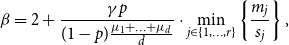 \begin{align*} \beta = 2 + \frac{\gamma p }{(1-p)\frac{\mu _1 + \ldots + \mu _d}{d}} \cdot \min _{j\in \{1,\ldots,r\}} \left \{\frac{m_j}{s_j} \right \}, \end{align*}
where  $s_j$ is the probability that by creating a new hyperedge a community
  $j$ is chosen as the one sharing it.
Proof. We need to prove that 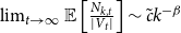 $\lim _{t \rightarrow \infty }{\mathbb{E}}\left [\frac{N_{k,t}}{|V_t|}\right ] \sim \tilde{c} k^{-\beta }$ for some constant
  $\tilde{c}$ and
  $\beta$ defined as in the statement of this theorem. By Lemma 1 (recall that since
  $|V_t|$ follows a binomial distribution, Lemma 1 holds also in case of
  $G_t$ if we replace
  $p_v+p_{ve}$ by
  $p$), it suffices to show
 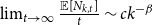 $\lim _{t \rightarrow \infty } \frac{{\mathbb{E}}[N_{k,t}]}{t} \sim c k^{-\beta }$ for some positive constant
  $c$. By Lemma 2:
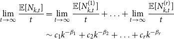 \begin{align*} \begin{split} \lim _{t \rightarrow \infty } \frac{{\mathbb{E}}[N_{k,t}]}{t} & = \lim _{t \rightarrow \infty } \frac{{\mathbb{E}}[N_{k,t}^{(1)}]}{t} + \ldots + \lim _{t \rightarrow \infty } \frac{{\mathbb{E}}[N_{k,t}^{(r)}]}{t} \\[5pt] & \sim c_1 k^{-\beta _1} + c_2 k^{-\beta _2} + \ldots + c_r k^{-\beta _r} \end{split} \end{align*}
for some constants  $c_1, \ldots, c_r$ and
  $\beta _j = 2 + \frac{\gamma \bar{V}_j}{\bar{D}_j}$. Thus
  $\lim _{t \rightarrow \infty } \frac{{\mathbb{E}}[N_{k,t}]}{t} \sim c k^{-\beta }$, where
 \begin{align*} \beta = \min _{j \in \{1,\ldots,r\}} \left \{\beta _j\right \}= 2 + \gamma \cdot \min _{j\in \{1,\ldots,r\}} \left \{ \frac{\bar{V}_j}{\bar{D}_j} \right \} = 2 + \frac{\gamma p }{(1-p)\frac{\mu _1 + \ldots + \mu _r}{r}} \cdot \min _{j\in \{1,\ldots,r\}} \left \{\frac{m_j}{s_j} \right \}. \end{align*}
5. Modularity of $\mathbf{G(G_0,p,M,X,P,\gamma )}$
In this section, we give lower bounds for the modularity of  $G = G(G_0,p,M,X,P,\gamma )$ in terms of the values from matrix
  $P$. We analyze
  $G=(V,E)$ obtained up to time
  $t$ (this time we omit superscripts t). Recall that each vertex from
  $V$ is assigned to one of
  $r$ communities,
  $V = C^{(1)} \mathbin{\dot{\cup }} C^{(2)} \mathbin{\dot{\cup }} \ldots \mathbin{\dot{\cup }} C^{(r)}$. We obtain the lower bound for modularity deriving the modularity score of the partition
  $\mathcal{C} = \{C^{(1)}, C^{(2)}, \ldots, C^{(r)}\}$. This choice of partition seems obvious provided that matrix
  $P$ is strongly assortative, that is, the probabilities of having a hyperedge inside communities are all bigger than the highest probability of having a hyperedge joining different communities. Note that what matters for the value of modularity is the total sum of degrees in each community, not the distribution of degrees. Therefore, we do not use the fact that the degree distribution follows a power-law in each community and in the whole model. We just use information from matrix
  $P$. Thus, in fact, we derive the lower bound for the modularity of a stochastic block model with
  $r$ communities. Recall that for
  $\ell \geqslant 1$
  $E_{\ell } \subseteq E$ is the set of hyperedges of cardinality
  $\ell$. First, we state general lower bound for the modularity of
  $G$ as a function of matrix
  $P$.
$P$.
Lemma 3. Let  $G = G(G_0,p,M,X,P,\gamma )$ with the size of each hyperedge bounded by
  $z$. Let
  $p_i$ be the probability that a randomly chosen hyperedge is within community
  $C^{(i)}$ (i.e. all vertices of a hyperedge belong to
  $C^{(i)}$). By
  $s_i$ we denote the probability that a randomly chosen hyperedge has at least one vertex in community
  $C^{(i)}$. Assume also that whp
  $|E_{\ell }|/|E| \sim a_{\ell }$ for some constants
  $a_{\ell } \in [0,1]$ and
  $vol(V)/|E| \sim \delta$ for some constant
  $\delta \in (0,\infty )$. Then whp
 \begin{align*} \lim _{t \rightarrow \infty } q^*(G) \geqslant (1+o(1)) \left (\sum _{i=1}^{r} p_i - \sum _{i=1}^{r} \sum _{\ell \geqslant 1} a_{\ell }\left (\frac{(z-1)s_i+p_i}{\delta }\right )^{\ell } \right ). \end{align*}
Remark 8. Note that for  $G$ being
  $2$-uniform (thus simply a graph) this result simplifies significantly to
  $\lim _{t \rightarrow \infty } q^*(G) \geqslant (1+o(1)) (\sum _{i=1}^{r} p_{i} - 1/4 \sum _{i=1}^{r}(s_i+p_{i})^2 )$.
Proof. Let  $\mathcal{C} = \{C^{(1)}, C^{(2)}, \ldots, C^{(r)}\}$. Let also
  $q$ denote the probability of adding a new hyperedge in a single time step (hence
  $q=1-p$, referring to notation from Section 4). Thus, whp
  $|E| \sim t \cdot q$ ("
 $\sim$" refers to the limit by
  $t\rightarrow \infty$). By Definition 2:
 \begin{align*} q^*(G) = \max _{\mathcal{A}} q_{\mathcal{A}}(G) \geqslant q_{\mathcal{C}}(G) = \sum _{i=1}^{r}\left (\frac{|E(C^{(i)})|}{|E|} - \sum _{\ell \geqslant 1}\frac{|E_{\ell }|}{|E|}\left (\frac{vol(C^{(i)})}{vol(V)}\right )^{\ell } \right ). \end{align*}
We obtain that with high probability
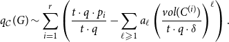 \begin{align*} q_{\mathcal{C}}(G) \sim \sum _{i=1}^{r}\left (\frac{t \cdot q \cdot p_{i}}{t \cdot q} - \sum _{\ell \geqslant 1}a_{\ell }\left (\frac{vol(C^{(i)})}{t \cdot q \cdot \delta }\right )^{\ell } \right ). \end{align*}
Note that if at a certain time step appears a hyperedge with all vertices contained in  $C^{(i)}$, which happens with probability
  $q \cdot p_{i}$, it adds up at most
  $z$ to
  $vol(C^{(i)})$. If at a certain time step appears a hyperedge joining at least
  $2$ communities with at least one vertex in
  $C^{(i)}$, which happens with probability
  $q (s_i-p_{i})$, it adds up at most
  $z-1$ to
  $vol(C^{(i)})$. Thus, whp
 \begin{align*} \begin{split} \lim _{t \rightarrow \infty } q^*(G) & \geqslant (1+o(1)) \left (\sum _{i=1}^{r} p_i - \sum _{i=1}^{r} \sum _{\ell \geqslant 1} a_{\ell }\left (\frac{t \cdot q \cdot (z p_i + (z-1)(s_i-p_i))}{t \cdot q \cdot \delta }\right )^{\ell } \right )\\[5pt] & = (1+o(1)) \left (\sum _{i=1}^{r} p_i - \sum _{i=1}^{r} \sum _{\ell \geqslant 1} a_{\ell }\left (\frac{(z-1)s_i+p_i}{\delta }\right )^{\ell } \right ). \end{split} \end{align*}
Remark 9. Note that the above result in most cases will not be tight. For example, the last inequality in the proof is tight only for graphs. Therefore, by some additional knowledge about the underlying hypergraph, one should be able to improve the bound. For example, assume that there is a node  $v$ (not alone in its community) with the property that all hyperedges containing this node also have some nodes from other communities. Such hyperedges do not influence the value of edge contribution (as none of them is entirely contained in one community). Therefore, putting the node
  $v$ to its own, separate community will increase the value of the modularity score (the edge contribution will not change while the degree tax will decrease).
Below we state the lower bound for the modularity of  $G$ in a version in which the knowledge of the whole matrix
  $P$ is not necessary. Instead, we use its two characteristics:
  $\alpha$—the probability that a randomly chosen hyperedge joins at least two different communities (may be interpreted as the amount of noise in the network) and
  $\beta$—the maximum value among
  $p_{i}$’s. The modularity of the model will be maximized for
  $\alpha =0$ (when there are no hyperedges joining different communities) and
  $\beta = 1/r$ (when all
  $p_{i}$’s are equal to
  $1/r$; thus, hyperedges are distributed uniformly across communities).
Lemma 4. By assumptions from Lemma 3 whp
 \begin{align*} \begin{split} \lim _{t \rightarrow \infty } & q^*(G) \geqslant (1+o(1)) \cdot \\[5pt] & \cdot \left (1-\alpha - a_1 \left (\frac{z}{\delta }\right )((z-2)\alpha +1) - \sum _{\ell \geqslant 2} a_{\ell }\left (\frac{z}{\delta }\right )^{\ell }\left ((r-1)\beta ^{\ell } + ((z-1)\alpha + \beta )^{\ell }\right ) \right ), \end{split} \end{align*}
where 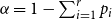 $\alpha = 1 - \sum _{i=1}^{r}p_{i}$ and
 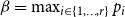 $\beta = \max _{i \in \{1,\ldots,r\}} p_{i}$.
Remark 10. For  $G$ being
  $2$-uniform, the result simplifies to
  $\lim _{t \rightarrow \infty } q^*(G) \geqslant (1+o(1)) (1 - r \beta ^2 - \alpha (1 + \alpha + 2\beta ) )$. Note that for
  $\alpha =0$ and
  $\beta =1/r$, this bound equals
  $1-1/r$ and is tight, that is, it is the modularity of the graph with the same number of edges in each of its
  $r$ communities and no edges between different communities.
Remark 11. Obtained bounds work well as long as the cardinalities of hyperedges do not differ too much. This is since deriving them we bound the cardinality of each hyperedge by the size of the biggest one. In particular, the bounds are very good in case of uniform hypergraphs (see Section 7).
Proof. Let 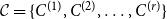 $\mathcal{C} = \{C^{(1)}, C^{(2)}, \ldots, C^{(r)}\}$ and for
  $i \in \{1,2,\ldots,r\}$ let
  $\tilde{s}_i$ be the probability that a randomly chosen hyperedge joins at least two communities and
  $C^{(i)}$ is one of them. Note that for
  $s_i$ defined as in Lemma 3 we get
  $s_i = \tilde{s}_i + p_i$. By Lemma 3 we get whp
 \begin{align} \begin{split} \lim _{t \rightarrow \infty } & q^*(G) \geqslant (1+o(1)) \cdot \\[5pt] & \cdot \left ( (1-\alpha ) - \frac{a_1}{\delta }\left ((z-1) \sum _{i=1}^{r} \tilde{s}_i + z \sum _{i=1}^{r} p_i \right ) - \sum _{\ell \geqslant 2} \frac{a_{\ell }}{\delta ^{\ell }} \sum _{i=1}^{r} ((z-1)\tilde{s}_i+zp_i)^{\ell } \right ). \end{split} \end{align}
Now, by  $r_k$ denote the probability that a randomly chosen hyperedge joins exactly
  $k$ communities. Note that
 \begin{align} \sum _{i=1}^{r} \tilde{s}_i = 2r_2 + 3r_3 + \ldots + zr_z \leqslant z(1 - \sum _{i=1}^{r} p_i) = z \alpha . \end{align}
Thus,
 \begin{align} \frac{a_1}{\delta } \left ((z-1) \sum _{i=1}^{r} \tilde{s}_i + z \sum _{i=1}^{r} p_i \right ) \leqslant a_1 \left (\frac{z}{\delta }\right )((z-2)\alpha +1) \end{align}
and
 \begin{align} \sum _{\ell \geqslant 2} \frac{a_{\ell }}{\delta ^{\ell }} \sum _{i=1}^{r} ((z-1)\tilde{s}_i +zp_i)^{\ell } \leqslant \sum _{\ell \geqslant 2} a_{\ell }\left (\frac{z}{\delta }\right )^{\ell }\left ((r-1)\beta ^{\ell } + ((z-1)\alpha + \beta )^{\ell }\right ). \end{align}
Plugging (3) and (4) into (1) we get the result. (See Section B in the Appendix for more details.)
6. Comparison with mixed preferential attachment model
The minority-majority graphs presented in Avin et al. (Reference Avin, Daltrophe, Keller, Lotker, Mathieu, Peleg and Pignolet2020), and (Reference Avin, Keller, Lotker, Mathieu, Peleg and Pignolet2015) are the only dynamic models we are aware of, featuring communities and power-law degree distribution. Therefore, we devote separate section for a comparison between them and our hypergraph  $G(G_0,p,M,X,P,\gamma )$. As a model presented in Avin et al. (Reference Avin, Keller, Lotker, Mathieu, Peleg and Pignolet2015) is a simpler version of a model from Avin et al. (Reference Avin, Daltrophe, Keller, Lotker, Mathieu, Peleg and Pignolet2020), we mainly refer to the latter one, denoting it by
  $G^*$.
6.1. Graph model $\mathbf{G^*(G^*_0,r,\delta,\rho _R,\rho _B)}$, (Avin et al., Reference Avin, Daltrophe, Keller, Lotker, Mathieu, Peleg and Pignolet2020])
In a mixed preferential attachment model  $G^*$, each vertex is assigned to exactly one of two communities. Each vertex, on its arrival, establishes connections with
  $\delta$ existing vertices. A preferential attachment rule is specific here, as it may be marked by homophily (when vertices tend to connect to others from the same community) or heterophily (when vertices prefer to join a different community).
Let  $r \in (0,1)$,
  $\rho _R,\rho _B \in [0,1]$, and
  $\delta \in \mathbb{N^{+}}$. Let
  $G^*_0$ be any graph with each vertex assigned either to the red or to the blue community. For
  $t \geq 0$,
  $G^*_{t+1}$ is constructed from
  $G^*_t=(V^*_t,E^*_t)$ as follows:
• A new vertex
$v$ arrives and is assigned to the red community with probability $r$ and to the blue community otherwise.-
• Repeat until
$\delta$ new edges are constituted:– choose a vertex
$u$ from $V^*_t$ in proportion to degrees (i.e. $\mathbb{P}[u \text{ is chosen}] = \frac{\deg _t(u)}{\sum _{v \in V^*_{t}}{(\deg _t(v))}}$);-
– assume that
$v$ is of color $x \in \{R,B\}$; if $u$ is of the same color then with probability $\rho _x$ it becomes a neighbor of $v$ in $G^*_{t+1}$; if $u$ is of different color it becomes a neighbor of $u$ in $G^*_{t+1}$ with probability $1-\rho _x$; multiedges are allowed (note that it may happen that no edge will be constituted in this single procedure step).


The case with  $\rho _R=\rho _B=1$ (thus when new connections appear only between vertices from the same community) is called a perfect homophily. On the other hand, by
  $\rho _R=\rho _B=0$ one talks about a perfect heterophily. Note also that the case
  $\rho _R=\rho _B=1/2$ (when the appearance of a new connection does not depend on the colors) reflects the Barabási-Albert model from Barabási & Albert (Reference Barabási and Albert1999).
Remark 12. In this section, we will concentrate only on the degree distribution results for  $G^*$. It is worth mentioning, however, that the paper (Avin et al., Reference Avin, Keller, Lotker, Mathieu, Peleg and Pignolet2015) studies the simpler version of
  $G^*$ in a very interesting context of a glass ceiling effect. Informally speaking, it verifies which mechanisms in social networks cause that the vertices of minority are not represented well among vertices of high degrees.
The mixed preferential attachment model  $G^*$ exhibits a power-law degree distribution for each community, possibly with different exponents, depending on
  $\rho _R,\rho _B$ and
  $r$.
$r$.
Theorem 3 (Theorem 2 in [4]). Consider a graph  $G^*=G^*(G^*_0,r,\delta,\rho _R,\rho _B)$ for any
  $t\gt 0$. The degree distributions of the red and the blue vertices follow a power-law with exponents
 \begin{align*} \beta _R = 1 + \frac{1}{C_R} \quad \quad \text{and} \quad \quad \beta _B = 1 + \frac{1}{C_B} \end{align*}
respectively, where
 \begin{align*} C_R & = \frac{1}{2} \left (\frac{(1-r)(1-\rho _B)}{\rho _B + \alpha - 2 \rho _B \alpha } + \frac{r \rho _R}{1-\rho _R-\alpha +2\rho _R \alpha }\right ), \\[5pt] C_B & = \frac{1}{2} \left (\frac{(1-r)\rho _B}{\rho _B + \alpha - 2 \rho _B \alpha } + \frac{r (1-\rho _R)}{1-\rho _R-\alpha +2\rho _R \alpha }\right ), \end{align*}
and  $\alpha$ is a unique real number in
  $(0,1)$ satisfying the equation
 \begin{align*} 2 \alpha = 1 + \frac{\rho _B(1-r)(1-\alpha )}{\rho _B(2 \alpha -1)-\alpha } + \frac{r \rho _R \alpha }{1-\alpha +\rho _R(2 \alpha -1)}. \end{align*}
Remark 13. The value  $\alpha$ has its interpretation in
  $G^*$, namely
 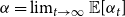 $\alpha = \lim _{t \rightarrow \infty }{\mathbb{E}}[\alpha _t]$, where
  $\alpha _t$ is the ratio of the sum of degrees of red vertices in
  $G^*_t$ to the sum of degrees of all vertices in
  $G^*_t$.
6.2. Comparison of $\mathbf{G^*}$ and $\mathbf{G}$


Let us now consult the similarities and differences between  $G^*$ and our model
  $G$. Definitely, both models grow with time and both of them exhibit a power-law degree distribution for each community. Moreover, note that the homophilic/heterophilic behavior of
  $G^*$ may be reflected in
  $G$ by a proper parameter assignment in matrix
  $P$. What differs
  $G^*$ from
  $G$ is that at time
  $t$ the model
  $G$ allows for inserting edges between vertices that appeared before time
  $t$, while in
  $G^*$ a new edge always attaches to a newly arrived vertex.
Nevertheless, we wanted to check whether it is possible to tune the parameters of  $G$ in a way which preserves the main characteristics of
  $G^*$ and gives the same exponents in the corresponding power-laws. Therefore for
  $G^* = G^*(G_0^*,r,\delta,\rho _R,\rho _B)$ we considered
  $G$ with the following parameters. The vector
  $M$ was chosen to be
  $M=[r,1-r]$ (reflecting the fractions of vertices in red and blue community, respectively),
  $p=1/(\delta +1)$ (preserving the ratio of
  $1$ vertex per
  $\delta$ edges), the vector
  $X$ was chosen to have all the hyperedges of cardinality
  $2$, the matrix
  $P$ was preserving the proper fractions of red-red, blue-blue, and red-blue edges (the calculations are given in the next paragraph), and
  $\gamma$ was left for an adjustment to (possibly) obtain the same exponents for the corresponding power-laws.
We figured out the reasonable parameters for the matrix  $P$ as follows. We obtained the limiting expected fraction of red-red edges in
  $G^*$ (denote it by
  $q_R$) using the concentration result for
  $\alpha _t$ from Lemma 7 in Avin et al. (Reference Avin, Daltrophe, Keller, Lotker, Mathieu, Peleg and Pignolet2020) and getting
 \begin{align*} q_R = r \cdot \alpha \cdot \rho _R + r \cdot \alpha \cdot f_R \cdot \rho _R + r \cdot \alpha \cdot f_R^2 \cdot \rho _R + \ldots = \frac{r \cdot \alpha \cdot \rho _R }{1-f_R} \end{align*}
where  $f_R = \alpha (1-\rho _R) + (1-\alpha )\rho _R$. Indeed,
  $r$ refers to the arrival of a new red vertex,
  $\alpha$ for a chance that a red vertex is chosen in a preferential selection and
  $\rho _R$ for a chance of constituting an edge between red vertices in a single procedure step. Next,
  $f_R$ is a probability that no edge will be constituted in a single procedure step, conditioned on the fact that a newly arrived vertex is red. Analogously, we got a limiting expected fraction of blue-blue edges in
  $G$ (denoted by
  $q_B$)
 \begin{align*} q_B = \frac{(1-r)(1-\alpha )\rho _B}{1-f_B}, \quad \text{where} \quad f_B = (1-\alpha )(1-\rho _B) + \alpha \cdot \rho _B. \end{align*}
Thus for red-blue edges in  $G$ (denoted by
  $q_{RB}$), we got
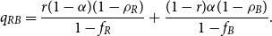 \begin{align*} q_{RB} = \frac{r(1-\alpha )(1-\rho _R)}{1-f_R} + \frac{(1-r)\alpha (1-\rho _B)}{1-f_B}. \end{align*}
Now, setting 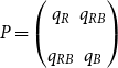 $P = \begin{pmatrix} q_R & q_{RB}\\[5pt] q_{RB} & q_B \end{pmatrix}$ we obtain the same limiting expected fraction of red-red, blue-blue, and red-blue edges in both models.
Having set all the parameters we could check whether the power-law exponents for  $G$ (from Theorem 2) overlap with the ones for
  $G^*$ (from Theorem 3). The answer is negative, that is, it is not possible to give the value of
  $\gamma$ such that for all
  $r\in (0,1)$ and for all
  $\rho _B,\rho _R \in [0,1]$ the corresponding power-law exponents of two models overlap. We have repeated similar calculations for
  $G$ being a
  $(\delta +1)$-uniform hypergraph (thus choosing
  $X$ such that all hyperedges were of size
  $\delta +1$ and
  $p=1/2$), and we also got a negative result.
We conclude that, despite many obvious similarities, models  $G$ and
  $G^*$ noticeably differ in their power-law behavior. We see the cause in the fact that
  $G^*$ does not allow for inserting edges between “old” vertices. The fact that adding this possibility influences a power-law exponent in a degree distribution was already observed by Cooper and Frieze in Cooper & Frieze (Reference Cooper and Frieze2003).
7. Experimental results
In this section, we show how the modularity of our model  $G$ compares with the ones of Avin et al., hypergraph
  $A$ (Avin et al., Reference Avin, Lotker, Nahum and Peleg2019) and of a real-life co-authorship graph
  $R$. We also check how good is our theoretical lower bound for modularity.
To build a real-life co-authorship hypergraph  $R$ we used data from the citation database Scopus (2019). These included articles across all disciplines from the years 1990-2018. As data were collected within the frame of the project investigating the impact of different sources of funding on French research, only papers with at least one French co-author were taken into consideration. Obtained hypergraph consisted of
  $\approx 2.2 \cdot 10^6$ nodes (authors) and
  $\approx 3.9 \cdot 10^6$ hyperedges (where a single hyperedge represented a set of co-authors of a particular article). We narrowed down our experiments just to the largest connected component keeping
  $94.22\%$ of nodes and
  $99.23\%$ of hyperedges.
To get a partition of  $R$ into communities, we used Leiden procedure (Traag et al., Reference Traag, Waltman and van Eck2019)—a popular community detection algorithm for large networks. Finding a partition maximizing modularity score is NP-hard (Brandes et al., Reference Brandes, Delling, Gaertler, Gorke, Hoefer, Nikoloski and Wagner2008). Leiden algorithm is nowadays one of the best heuristics trying to do that. Therefore, we treat its outcome partition as the one whose modularity score is a quite precise approximation of the modularity of graphs in question. Leiden algorithm was run on the flattened (
 $2$-section) hypergraph, that is, a graph obtained from a hypergraph by exchanging hyperedges with cliques. It identified
  $595$ communities. The modularity score of the obtained partition, calculated according to the definition of modularity for hypergraphs (Definition 2), was approximately
  $0.63$.
Remark 14. Initially, to get a community structure of  $R$, we tried to use the algorithm dedicated directly for hypergraphs and using hypergraph modularity, (Kamiński et al., Reference Kamiński, Poulin, Prałat, Szufel and Théberge2019; Kamiński et al., Reference Kamiński, Prałat and Théberge2021; Antelmi et al., Reference Antelmi, Cordasco, Kamiński, Prałat, Scarano, Spagnuolo and Szufel2020). Unfortunately, we were forced to resign due to the big scale of the hypergraph
  $R$ and our technical limitations.
For the rest of the study, we decided to keep only the communities with at least one hundred nodes. This eliminated only  $0.44\%$ of the authors and resulted in
  $R$ having
  $47$ meaningful communities. In Figure 1, one finds the distribution of their sizes. Figure 2 presents the log-log plots of the complementary cumulative distribution functions of degrees in the whole
  $R$ and its three largest communities. One may notice that their characters are similar. They resemble a power-law only piecewise; thus, probably a broken power-law (i.e. the piecewise function consisting of different power-laws) or a power-law with an exponential cutoff could give a good fit here.

Figure 1. Distribution of the sizes of  $47$ largest communities in
  $R$ identified by Leiden algorithm. The numbers indicate the fraction of the nodes from a given community with respect to the total number of nodes in
  $47$ largest communities.
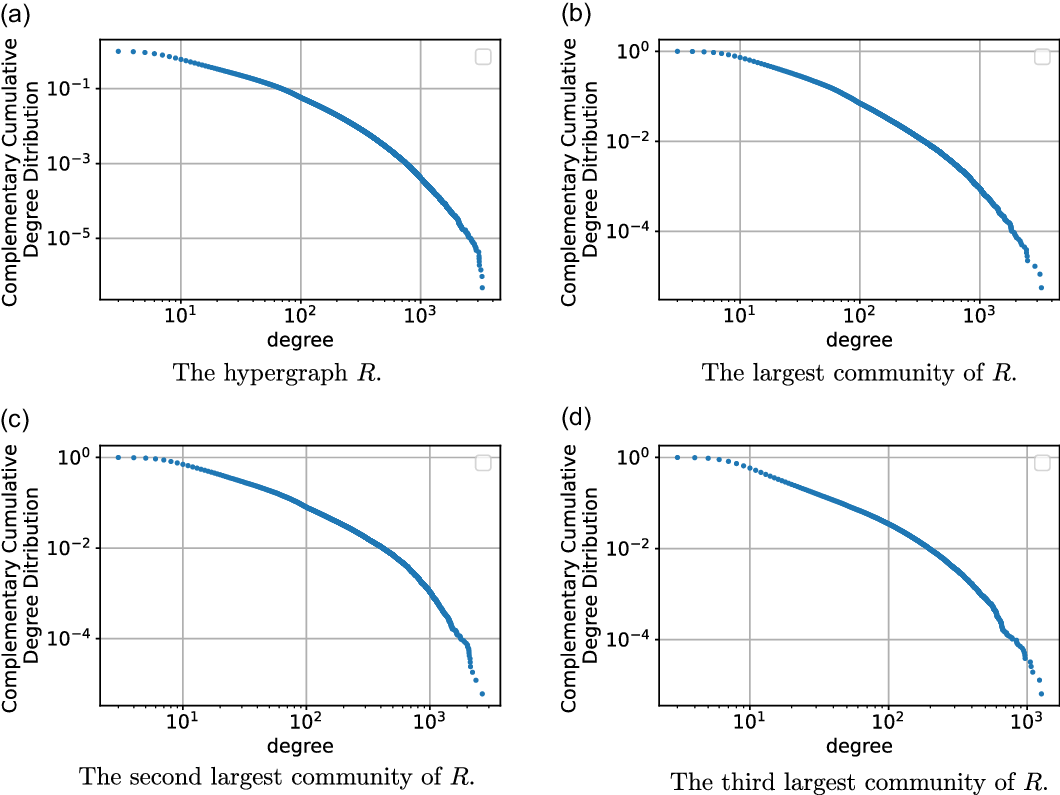
Figure 2. The log-log plots of the complementary cumulative distribution functions of the degrees in  $R$.
$R$.
Next, we implemented our model  $G$ and Avin’s et al., model
  $A$ using the parameters (distribution of sizes of hyperedges,
  $M$,
$M$,  $P$) gathered from
  $R$. Our theoretical model
  $G$ features a power-law degree distribution (compare Figure 3) which is commonly expected from the models mirroring the real-life complex networks. Upgrading the model to obtain a broken power-law or an exponential cutoff in its degree distribution (e.g. including aging or deactivating of vertices) is left as a future work. Figure 4 compares the modularities of
  $G$,
$G$,  $A$, and
  $R$ (the modularities of
  $G$ and
  $A$ were approximated using the same method as for
  $R$). For
  $R$ the value
  $\alpha$ equals
  $0.21$. Then, the modularity of our model
  $G$ is around
  $0.69$ which is very close to the modularity of
  $R$ (
$R$ ( $\approx 0.63$). The modularity of
  $A$ is very low (
 $\approx 0.06$), as
  $A$ does not feature communities. Figure 4 also shows how the modularity of
  $G$ changes with
  $\alpha$ and one may notice that it stays at reasonably a high level even when the number of hyperedges involving two communities increase leading to a network less distinctly partitioned.
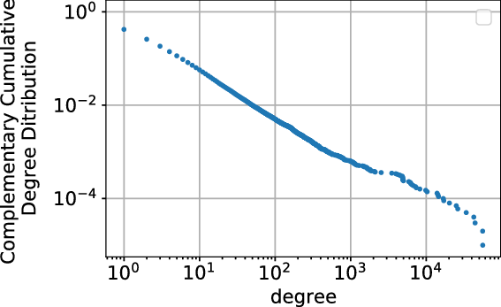
Figure 3. The log-log plot of the complementary cumulative distribution function of the degrees in the theoretical model  $G$,
$G$,  $t=10^5$.
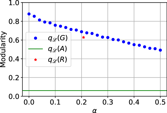
Figure 4. Comparison of the modularity between our model  $G$, Avin et al., hypergraph
  $A$ and the real co-authorship hypergraph
  $R$.
$R$.
Finally, we wanted to confirm experimentally that our theoretical lower bounds for modularity are indeed very good for uniform hypergraphs following our theoretical model. Figure 5(a) and 5(b) shows the lower bound from 3 in comparison with the modularity of  $2$- and
  $20$-uniform hypergraphs
  $\tilde{G}(\tilde{G}_0,p,M,X,P,\gamma )$ on
  $10^4$ vertices, where
  $M$ is uniform and of size
  $47$ (the choice of
  $47$ communities may be treated here as random; however, it was obviously inspired by the previous experiments on real data) and the matrix
  $P$ has values
  $(1-\alpha )/47$ on the diagonal and the rest of its probability mass is spread uniformly over the remaining entries.
  $M$ and
  $P$ were chosen such to deal with a possibly regular model in which we could control by a single parameter
  $\alpha$ the fraction of hyperedges that are spread across more than one community. Note that
  $1-\alpha$ is the probability that a randomly chosen hyperedge is all contained within a single community, that is,
  $\alpha$ measures the amount of noise in the network. As we expected, in this regular regime, the theoretical bound almost overlapped with the value of modularity.
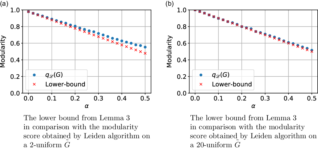
Figure 5. Experimental results on modularity.
8. Conclusion and further work
We have theoretically proved and experimentally confirmed that our model exhibits high modularity, which is rare for known preferential attachment graphs and was not present in hypergraph models so far. While our model has many parameters and may seem complicated, this general formulation allowed us to unify many results known so far. Moreover, it can be easily transformed into much simpler models (e.g. by setting some arguments trivially to  $0$, repeating the same distributions for hyperedges cardinalities, etc).
Our model exhibits power-law degree distribution. However, many real networks in fact present an exponential cutoff in their degree distribution. One possible reason to explain this phenomenon is that nodes eventually become inactive. As further work, we plan to include this process in our model. The other direction of future study is making the preferential attachment depending not only on the degrees of the vertices but also on their own characteristic (generally called fitness (Borgs et al., Reference Borgs, Chayes, Constantinos and Roch2007)).
Data availability statement
The used dataset is a property of SCOPUS and cannot be distributed. We accessed it through a paid subscription.
Funding statement
This research was supported by grant SNIF (Scientific Networks and IDEX funding); and French Agence Nationale de la Recherche ANR (UCA JEDI Investments in the Future, grant number ANR-15-IDEX-01), (EUR DS4H, grant number ANR-17-EURE-004), (Digraphs, grant number ANR-19-CE48-0013).
Competing interests
None.
A. Degree distribution of $\mathbf{H(H_0,p,Y,X,m,\gamma )}$

The number of vertices in  $H_t$ is a random variable following a binomial distribution. Since
  $|V_0|=1$ we have
  $|V_t| \sim B(t,p_v+p_{ve}) + 1$. Since
  $|E_0|=1$, the number of hyperedges in
  $H_t$ is a random variable satisfying
  $|E_t| \sim m B(t,p_{ve}+p_e) + 1$.
Before we prove Theorem 1, we discuss briefly the concentration of random variables  $|V_t|$ (the number of vertices at time
  $t$),
$t$),  $D_t$ (the sum of degrees at time
  $t$) and
  $W_t = D_{t} + \gamma |V_t|$. We start with a couple of technical lemmas that will be helpful later on.
Lemma 5 (Chernoff bounds, [37], Chapter 4.2). Let  $Z_1,Z_2,\ldots,Z_t$ be independent indicator random variables with
  $\mathbb{P}[Z_i=1]=p_i$ and
  $\mathbb{P}[Z_i=0]=1-p_i$. Let
  $\delta \gt 0$,
  $Z = \sum _{i=1}^{t} Z_i$ and
  $\mu ={\mathbb{E}}[Z] = \sum _{i=1}^{t} p_i$. Then
 \begin{align*} \mathbb{P}[|Z-\mu | \geqslant \delta \mu ] \leq 2 e^{-\mu \delta ^2/3}. \end{align*}
Corollary 1. Since 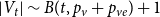 $|V_t| \sim B(t,p_v+p_{ve}) + 1$ setting
  $\delta = \sqrt{\frac{9 \ln{t}}{(p_v+p_{ve})t}}$ in Lemma 5, we get
 \begin{align*} \mathbb{P}[||V_t|-{\mathbb{E}}[|V_t|]]| \geqslant \sqrt{9 (p_v+p_{ve}) t \ln{t}}] \leq 2/t^3. \end{align*}
Now, let us restate Lemma 1 and present its proof.
Lemma 1. If  $\lim _{t \rightarrow \infty } \frac{{\mathbb{E}}[N_{k,t}]}{t} \sim c k^{-\beta }$ for some positive constant
  $c$ then
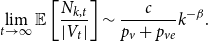 \begin{align*} \lim _{t \rightarrow \infty }{\mathbb{E}}\left [\frac{N_{k,t}}{|V_t|}\right ] \sim \frac{c}{p_v+p_{ve}} k^{-\beta }. \end{align*}
(Here “  $\sim$” refers to the limit by
  $k \rightarrow \infty$.)
Proof. Let  $(\Omega,{\mathcal{F}}, \mathbb{P})$ be the probability space on which random variables
  $N_{k,t}$ and
  $|V_t|$ are defined. Thus,
  $N_{k,t}\;:\;\Omega \rightarrow \mathbb{R}$ and
  $|V_t|\;:\;\Omega \rightarrow \mathbb{R}$. Let
  $\Omega _1 \subseteq \Omega$ denote the set of all
  $\omega \in \Omega$ such that
  $|V_t|(\omega ) \in ({\mathbb{E}}|V_t|-\sqrt{9 (p_v+p_{ve}) t \ln{t}},{\mathbb{E}}|V_t|+\sqrt{9 (p_v+p_{ve}) t \ln{t}})$. By Corollary 1, we know that
 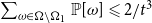 $\sum _{\omega \in \Omega \setminus \Omega _1} \mathbb{P}[\omega ] \leqslant 2/t^3$. Using the fact that for each
  $\omega$
  $\frac{N_{k,t}(\omega )}{|V_t|(\omega )} \leqslant 1$, we get
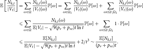 \begin{align*} \begin{split}{\mathbb{E}}\left [\frac{N_{k,t}}{|V_t|}\right ] & = \sum _{\omega \in \Omega } \frac{N_{k,t}(\omega )}{|V_t|(\omega )}\mathbb{P}[\omega ] = \sum _{\omega \in \Omega _1} \frac{N_{k,t}(\omega )}{|V_t|(\omega )}\mathbb{P}[\omega ] + \sum _{\omega \in \Omega \setminus \Omega _1} \frac{N_{k,t}(\omega )}{|V_t|(\omega )}\mathbb{P}[\omega ] \\[5pt] & \leqslant \sum _{\omega \in \Omega } \frac{N_{k,t}(\omega )}{{\mathbb{E}}|V_t|-\sqrt{9 (p_v+p_{ve}) t \ln{t}}}\mathbb{P}[\omega ] + \sum _{\omega \in \Omega \setminus \Omega _1} 1 \cdot \mathbb{P}[\omega ] \\[5pt] & \leqslant \frac{{\mathbb{E}}[N_{k,t}]}{{\mathbb{E}}|V_t|-\sqrt{9 (p_v+p_{ve}) t \ln{t}}} + 2/t^3 \sim \frac{{\mathbb{E}}[N_{k,t}]}{(p_v + p_{ve})t}. \end{split} \end{align*}
On the other hand, since  $N_{k,t} \leq t$,
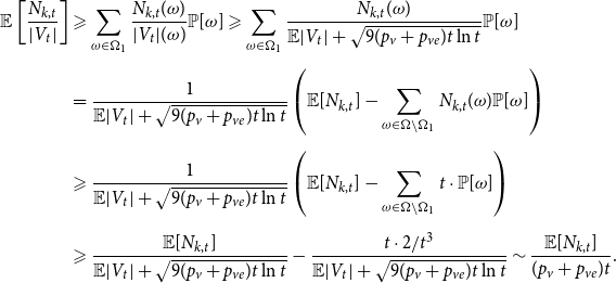 \begin{align*} \begin{split}{\mathbb{E}}\left [\frac{N_{k,t}}{|V_t|}\right ] & \geqslant \sum _{\omega \in \Omega _1} \frac{N_{k,t}(\omega )}{|V_t|(\omega )}\mathbb{P}[\omega ] \geqslant \sum _{\omega \in \Omega _1} \frac{N_{k,t}(\omega )}{{\mathbb{E}}|V_t|+\sqrt{9 (p_v+p_{ve}) t \ln{t}}}\mathbb{P}[\omega ] \\[5pt] & = \frac{1}{{\mathbb{E}}|V_t|+\sqrt{9 (p_v+p_{ve}) t \ln{t}}} \left ({\mathbb{E}}[N_{k,t}] - \sum _{\omega \in \Omega \setminus \Omega _1} N_{k,t}(\omega ) \mathbb{P}[\omega ]\right ) \\[5pt] & \geqslant \frac{1}{{\mathbb{E}}|V_t|+\sqrt{9 (p_v+p_{ve}) t \ln{t}}} \left ({\mathbb{E}}[N_{k,t}] - \sum _{\omega \in \Omega \setminus \Omega _1} t \cdot \mathbb{P}[\omega ]\right ) \\[5pt] & \geqslant \frac{{\mathbb{E}}[N_{k,t}]}{{\mathbb{E}}|V_t|+\sqrt{9 (p_v+p_{ve}) t \ln{t}}} - \frac{t \cdot 2/t^3}{{\mathbb{E}}|V_t|+\sqrt{9 (p_v+p_{ve}) t \ln{t}}} \sim \frac{{\mathbb{E}}[N_{k,t}]}{(p_v + p_{ve})t}. \end{split} \end{align*}
Lemma 6 (Hoeffding’s inequality, [22]). Let  $Z_1, Z_2, \ldots, Z_t$ be independent random variables such that
  $\mathbb{P}[Z_i \in [a_i,b_i]] =1$. Let
  $\delta \gt 0$ and
  $Z = \sum _{i=1}^{t}Z_i$. Then
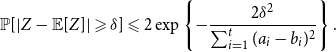 \begin{align*} \mathbb{P}[|Z -{\mathbb{E}}[Z]| \geqslant \delta ] \leqslant 2 \exp \left \{-\frac{2 \delta ^2}{\sum _{i=1}^t(a_i-b_i)^2}\right \}. \end{align*}
Lemma 7. Let  $t\gt 0$. Let
  ${\mathbb{E}}[Y_t] = \mu _0$, and
  ${\mathbb{E}}[X_t^{(i)}] = \mu _i$ for
  $i \in \{1,2,\ldots,r\}$. Moreover, let
  $2 \leqslant Y_t \lt t^{1/4}$ and
  $1 \leqslant X_t^{(i)} \lt t^{1/4}$ for
  $i \in \{1,2,\ldots,r\}$. Let
  $W_t = D_t + \gamma |V_t|$. Then
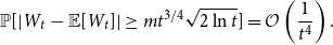 \begin{align*} \mathbb{P}[|W_t -{\mathbb{E}}[W_t]| \geq m t^{3/4}\sqrt{2\ln{t}}] = \mathcal{O}\left (\frac{1}{t^4}\right ). \end{align*}
Proof. Our initial hypergraph consists of a single hyperedge of cardinality  $1$ over a single vertex; thus,
  $W_0 = \gamma + 1$. For
  $t \geq 1$, we can obtain
  $W_t$ from
  $W_{t-1}$ by adding:
(1) either
$\gamma$ with probability $p_v$,-
(2) or
$\gamma + m Y_t$ with probability $p_{ve}$, -
(3) or
$m X_t^{(1)}$ with probability $p_e^{(1)}$, -
(4) or
$\ldots$, -
(5) or
$m X_t^{(r)}$ with probability $p_e^{(r)}$, -
(6) or
$0$ with probability $1-p_v-p_{ve}-p_e$.


Thus, we can express  $W_t$ as the sum of independent random variables
  $W_t = \gamma + 1 + Z_1 + Z_2 + \ldots + Z_t$, where
  ${\mathbb{E}}[Z_i] = \gamma \bar{V} + \bar{D}$ and
  $1 \leqslant Z_i \leqslant m t^{1/4} + \gamma$ for
  $i \in \{1,2,\ldots,t\}$ and
  $\bar{D}$ and
  $\bar{V}$ are defined as in Theorem 1:
 \begin{align*} \bar{V} = p_v+p_{ve} \quad \text{and} \quad \bar{D} = m(p_{ve}\mu _0 + p_e^{(1)}\mu _1 + \ldots + p_e^{(r)}\mu _r). \end{align*}
Now, setting  $\delta = m t^{3/4}\sqrt{2 \ln{t}}$ in Hoeffding’s inequality (see Lemma 6) we get
 \begin{align*} \mathbb{P}[|W_t -{\mathbb{E}}[W_t]| \geqslant m t^{3/4}\sqrt{2 \ln{t}}] \leqslant 2 \exp \left \{-\frac{4 \cdot m^2 \cdot t^{6/4} \cdot \ln{t}}{(t+1) (m \cdot t^{1/4} + \gamma )^2}\right \} = \mathcal{O}\left (\frac{1}{t^4}\right ). \end{align*}
Lemma 8 ([15], Chapter 3.3). Let  $\{a_t\}$ be a sequence satisfying the recursive relation
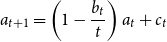 \begin{align*} a_{t+1} = \left (1-\frac{b_t}{t}\right )a_t + c_t \end{align*}
where  $b_t \xrightarrow{t \rightarrow \infty } b\gt 0$ and
  $c_t \xrightarrow{t \rightarrow \infty } c$. Then, the limit
  $\lim _{t \rightarrow \infty } \frac{a_t}{t}$ exists and
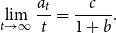 \begin{align*} \lim _{t \rightarrow \infty } \frac{a_t}{t} = \frac{c}{1+b}. \end{align*}
Now we are ready to give a detailed proof of Theorem 1.
Proof of Theorem 1. Here we take a standard master equation approach that can be found, for example, in Chung and Lu book [15] about complex networks or Avin et al., paper [5] on preferential attachment hypergraphs.
Recall that  $N_{k,t}$ denotes the number of vertices of degree
  $k$ at time
  $t$. We need to show that
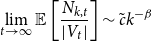 \begin{align*} \lim _{t \rightarrow \infty }{\mathbb{E}}\left [\frac{N_{k,t}}{|V_t|}\right ] \sim \tilde{c} k^{-\beta } \end{align*}
for some constant  $\tilde{c}$ and
 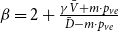 $\beta = 2+\frac{\gamma \bar{V} + m \cdot p_{ve}}{\bar{D} - m \cdot p_{ve}}$. However, by Lemma 1 we know that it suffices to show that
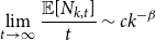 \begin{align*} \lim _{t \rightarrow \infty } \frac{{\mathbb{E}}[N_{k,t}]}{t} \sim c k^{-\beta } \end{align*}
for some constant  $c$.
$c$.
Our initial hypergraph  $H_0$ consists of a single hyperedge of cardinality
  $1$ over a single vertex; thus; we can write
  $N_{0,0} = 0$ and
  $N_{1,0}=1$. Now, to formulate a recurrent master equation we make the following observation for
  $t \geqslant 1$. The vertex
  $v$ has degree
  $k$ at time
  $t$ if either it had degree
  $k$ at time
  $t-1$ and was not chosen to any new hyperedge or it had degree
  $k-i$ at time
  $t-1$ and was chosen
  $i$ times to new hyperedges. Note that
  $i$ can be at most
  $\min \{k,mZ_t\}$, where
  $Z_t$ represents a random variable chosen among
  $Y_t, X_t^{(1)}, \ldots, X_t^{(r)}$ according to
 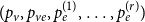 $(p_v,p_{ve},p_e^{(1)},\ldots,p_e^{(r)})$. Additionally, at each time step a vertex of degree
  $0$ may appear as the new one with probability
  $p_v$ and a vertex of degree
  $m$ may appear as the new one with probability
  $p_{ve}$. Let
  ${\mathcal{F}}_t$ be the
  $\sigma$-algebra associated with the probability space at time
  $t$. Let
  $Q_{d,k,t}$ denote the probability that a specific vertex of degree
  $k$ was chosen
  $d$ times to be included in new hyperedges at time
  $t$ (this probability is expressed as a random variable since it depends on a specific realization of the process up to time
  $t-1$). Let also
  $W_t = D_{t}+\gamma |V_{t}|$. For
  $t \geqslant 1$ we get
 \begin{align*}{\mathbb{E}}[N_{0,t} |{\mathcal{F}}_{t-1}] = p_v + N_{0,t-1} Q_{0,0,t} \end{align*}
and when  $k \geqslant 1$
 \begin{align*}{\mathbb{E}}[N_{k,t} |{\mathcal{F}}_{t-1}] = \delta _{k,m} p_{ve} + N_{k,t-1} Q_{0,k,t} + N_{k-1,t-1} Q_{1,k-1,t} \quad + \sum _{i=2}^{\min \{k,mZ_t\}} N_{k-i,t-1} Q_{i,k-i,t}, \end{align*}
where  $\delta _{k,m}$ is the Kronecker delta. We have extracted the first two terms in the above sum since below we prove that these are the dominating terms. Taking expectation on both sides, we obtain
 \begin{align} {\mathbb{E}}[N_{0,t}] = p_v +{\mathbb{E}}[N_{0,t-1} Q_{0,0,t}] \end{align}
and for  $k \geqslant 1$
 \begin{align} {\mathbb{E}}[N_{k,t}] = \delta _{k,m} p_{ve} +{\mathbb{E}}[N_{k,t-1} Q_{0,k,t}] +{\mathbb{E}}[N_{k-1,t-1} Q_{1,k-1,t}] \quad + \sum _{i=2}^{\min \{k,mZ_t\}}{\mathbb{E}}[N_{k-i,t-1} Q_{i,k-i,t}]. \end{align}
Note that
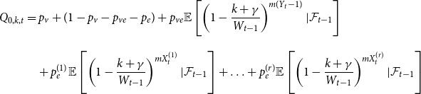 \begin{align*} \begin{split} Q_{0,k,t} & = p_v + (1-p_v-p_{ve}-p_e) + p_{ve}{\mathbb{E}}\left [\left (1-\frac{k+\gamma }{W_{t-1}}\right )^{m (Y_t-1)}|{\mathcal{F}}_{t-1}\right ]\\[9pt] & \quad + p_e^{(1)}{\mathbb{E}} \left [\left (1-\frac{k+\gamma }{W_{t-1}}\right )^{m X_t^{(1)}}|{\mathcal{F}}_{t-1}\right ] + \ldots + p_e^{(r)}{\mathbb{E}} \left [\left (1-\frac{k+\gamma }{W_{t-1}}\right )^{m X_t^{(r)}}|{\mathcal{F}}_{t-1}\right ] \end{split} \end{align*}
while for  $i \in \{1,2,\ldots,k\}$
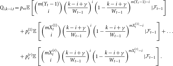 \begin{align*} \begin{split} Q_{i,k-i,t} & = p_{ve}{\mathbb{E}}\left [\binom{m(Y_t-1)}{i}\left (\frac{k-i+\gamma }{W_{t-1}}\right )^i\left (1-\frac{k-i+\gamma }{W_{t-1}}\right )^{m(Y_t-1)-i} |{\mathcal{F}}_{t-1}\right ] \\[9pt] & \quad + p_e^{(1)}{\mathbb{E}}\left [ \binom{m X_t^{(1)}}{i}\left (\frac{k-i+\gamma }{W_{t-1}}\right )^i\left (1-\frac{k-i+\gamma }{W_{t-1}}\right )^{m X_t^{(1)}-i} |{\mathcal{F}}_{t-1} \right ] + \ldots \\[9pt] & \quad + p_e^{(r)}{\mathbb{E}}\left [\binom{m X_t^{(r)}}{i}\left (\frac{k-i+\gamma }{W_{t-1}}\right )^i\left (1-\frac{k-i+\gamma }{W_{t-1}}\right )^{m X_t^{(r)}-i} |{\mathcal{F}}_{t-1}\right ]. \end{split} \end{align*}
Now, for any random variable  $Z_t$ with constant expectation
  $\mu$, independent of the
  $\sigma$-algebra
  ${\mathcal{F}}_{t-1}$, and such that
  $1 \leq Z_t \lt t^{1/4}$, by Bernoulli’s inequality we have
 \begin{align} \begin{split}{\mathbb{E}}\left [\left (1-\frac{k+\gamma }{W_{t-1}}\right )^{m Z_t}|{\mathcal{F}}_{t-1}\right ] & \geqslant{\mathbb{E}}\left [\left (1-\frac{mZ_t(k+\gamma )}{W_{t-1}}\right )|{\mathcal{F}}_{t-1}\right ] = 1 - \frac{m\mu (k+\gamma )}{W_{t-1}}. \end{split} \end{align}
On the other hand (using the fact that for  $x \in [0,1]$ and
  $n \in \mathbb{N}$ we have
  $(1-x)^n \leq \frac{1}{1+nx}$),
 \begin{align} \begin{split}{\mathbb{E}}\left [\left (1-\frac{k+\gamma }{W_{t-1}}\right )^{m Z_t}|{\mathcal{F}}_{t-1}\right ] & \leqslant{\mathbb{E}}\left [\frac{1}{1+\frac{mZ_t(k+\gamma )}{W_{t-1}}}|{\mathcal{F}}_{t-1}\right ] \\[5pt] & ={\mathbb{E}}\left [1-\frac{mZ_t(k+\gamma )}{W_{t-1}+mZ(k+\gamma )}|{\mathcal{F}}_{t-1}\right ] \\[5pt] & \leqslant{\mathbb{E}}\left [1-\frac{mZ_t(k+\gamma )}{W_{t-1}} + \frac{(mZ_t(k+\gamma ))^2}{W_{t-1}^2}|{\mathcal{F}}_{t-1}\right ] \\[5pt] & \leqslant 1 - \frac{m\mu (k+\gamma )}{W_{t-1}} + \frac{t^{1/2}(m(k+\gamma ))^2}{W_{t-1}^2}, \end{split} \end{align}
where the last inequality follows from the assumption  $Z_t \lt t^{1/4}$. Now, let us consider the master equation (6) for
  ${\mathbb{E}}[N_{k,t}]$ term by term. We start with the expected number of vertices that had degree
  $k$ at time
  $t-1$ and are still of degree
  $k$ at time
  $t$. By (7), Lemma 7 and the fact that
  $N_{k,t-1} \leq t$ we get
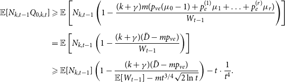 \begin{align*} \begin{split}{\mathbb{E}}[N_{k,t-1} Q_{0,k,t}] & \geqslant{\mathbb{E}}\left [N_{k,t-1} \left (1 - \frac{(k+\gamma ) m (p_{ve}(\mu _0-1) + p_e^{(1)}\mu _1 + \ldots + p_e^{(r)}\mu _r)}{W_{t-1}} \right )\right ] \\[5pt] & ={\mathbb{E}}\left [N_{k,t-1} \left (1 - \frac{(k+\gamma ) (\bar{D}-mp_{ve})}{W_{t-1}} \right )\right ] \\[5pt] & \geqslant{\mathbb{E}}[N_{k,t-1}] \left (1 - \frac{(k+\gamma ) (\bar{D}-mp_{ve})}{{\mathbb{E}}[W_{t-1}]-mt^{3/4}\sqrt{2 \ln{t}}}\right ) - t \cdot \frac{1}{t^4}. \end{split} \end{align*}
To get the last inequality, one needs to conduct calculations analogous to those from the proof of Lemma 1. By 8 and additionally using the fact that  $W_{t-1} \geq 1$
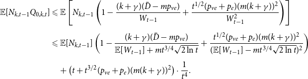 \begin{align*} \begin{split}{\mathbb{E}}[N_{k,t-1} Q_{0,k,t}] & \leqslant{\mathbb{E}}\left [N_{k,t-1} \left (1 - \frac{(k+\gamma ) (\bar{D}-mp_{ve})}{W_{t-1}} + \frac{t^{1/2}(p_{ve}+p_e)(m(k+\gamma ))^2}{W_{t-1}^2}\right )\right ] \\[5pt] & \leqslant{\mathbb{E}}[N_{k,t-1}] \left (1-\frac{(k+\gamma ) (\bar{D}-mp_{ve})}{{\mathbb{E}}[W_{t-1}]+mt^{3/4}\sqrt{2 \ln{t}}}+\frac{t^{1/2}(p_{ve}+p_e)(m(k+\gamma ))^2}{({\mathbb{E}}[W_{t-1}]-mt^{3/4}\sqrt{2 \ln{t}})^2} \right ) \\[5pt] & \quad + \left (t + t^{3/2}(p_{ve}+p_e)(m(k+\gamma ))^2\right ) \cdot \frac{1}{t^4}. \end{split} \end{align*}
Again, for the last inequality, proceed as in the proof of Lemma 1. Since  ${\mathbb{E}}[W_{t-1}] = \bar{D}(t-1) + \gamma \bar{V}(t-1)$ and
  ${\mathbb{E}}[N_{k,t-1}] \leqslant t$, we obtain for fixed
  $k$
$k$
 \begin{align} {\mathbb{E}}[N_{k,t-1} Q_{0,k,t}] ={\mathbb{E}}[N_{k,t-1}] \left (1 - \frac{(k+\gamma ) (\bar{D}-mp_{ve})}{t(\bar{D} + \gamma \bar{V})+\mathcal{O}(t^{3/4}\sqrt{\ln{t}})}\right ) +{\mathcal{O}}\left (\frac{1}{\sqrt{t}}\right ). \end{align}
We treat 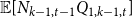 ${\mathbb{E}}[N_{k-1,t-1} Q_{1,k-1,t}]$ similarly. On one hand we have
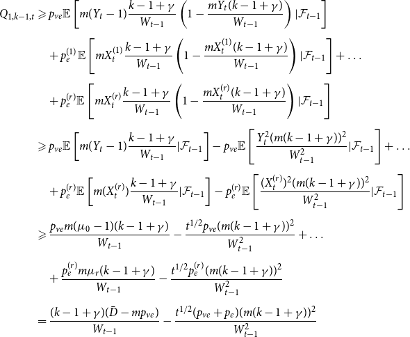 \begin{align*} \begin{split} Q_{1,k-1,t} & \geqslant p_{ve}{\mathbb{E}}\left [m(Y_t-1)\frac{k-1+\gamma }{W_{t-1}}\left (1-\frac{mY_t(k-1+\gamma )}{W_{t-1}} \right )|{\mathcal{F}}_{t-1}\right ] \\[5pt] & \quad + p_{e}^{(1)}{\mathbb{E}}\left [mX_t^{(1)}\frac{k-1+\gamma }{W_{t-1}}\left (1-\frac{mX_t^{(1)}(k-1+\gamma )}{W_{t-1}} \right )|{\mathcal{F}}_{t-1}\right ] + \ldots \\[5pt] & \quad + p_{e}^{(r)}{\mathbb{E}}\left [mX_t^{(r)}\frac{k-1+\gamma }{W_{t-1}}\left (1-\frac{mX_t^{(r)}(k-1+\gamma )}{W_{t-1}} \right )|{\mathcal{F}}_{t-1}\right ] \\[5pt] & \geqslant p_{ve}{\mathbb{E}}\left [m(Y_t-1)\frac{k-1+\gamma }{W_{t-1}}|{\mathcal{F}}_{t-1}\right ] - p_{ve}{\mathbb{E}}\left [\frac{Y_t^2(m(k-1+\gamma ))^2}{W_{t-1}^2} |{\mathcal{F}}_{t-1}\right ] + \ldots \\[5pt] & \quad + p_{e}^{(r)}{\mathbb{E}}\left [m(X_t^{(r)})\frac{k-1+\gamma }{W_{t-1}}|{\mathcal{F}}_{t-1}\right ] - p_{e}^{(r)}{\mathbb{E}}\left [\frac{(X_t^{(r)})^2(m(k-1+\gamma ))^2}{W_{t-1}^2} |{\mathcal{F}}_{t-1}\right ] \\[5pt] & \geqslant \frac{p_{ve}m(\mu _0-1)(k-1+\gamma )}{W_{t-1}} - \frac{t^{1/2}p_{ve}(m(k-1+\gamma ))^2}{W_{t-1}^2} + \ldots \\[5pt] & \quad + \frac{p_{e}^{(r)}m\mu _r(k-1+\gamma )}{W_{t-1}} - \frac{t^{1/2}p_{e}^{(r)}(m(k-1+\gamma ))^2}{W_{t-1}^2} \\[5pt] & = \frac{(k-1+\gamma )(\bar{D}-mp_{ve})}{W_{t-1}} - \frac{t^{1/2}(p_{ve}+p_e)(m(k-1+\gamma ))^2}{W_{t-1}^2} \end{split} \end{align*}
(the last inequality follows from assumptions  $Y_t \lt t^{1/4}$ and
  $X_t^{(i)}\lt t^{1/4}$), while on the other
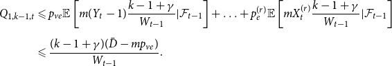 \begin{align*} \begin{split} Q_{1,k-1,t} & \leqslant p_{ve}{\mathbb{E}}\left [m(Y_t-1)\frac{k-1+\gamma }{W_{t-1}}|{\mathcal{F}}_{t-1}\right ] + \ldots + p_{e}^{(r)}{\mathbb{E}}\left [mX_t^{(r)}\frac{k-1+\gamma }{W_{t-1}}|{\mathcal{F}}_{t-1}\right ] \\[5pt] & \leqslant \frac{(k-1+\gamma )(\bar{D}-mp_{ve})}{W_{t-1}}. \end{split} \end{align*}
Again, by Lemma 7, the fact that  $N_{k-1,t-1} \leqslant t$ and
 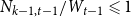 $N_{k-1,t-1}/W_{t-1}\leqslant 1$ for fixed
  $k$ we get
 \begin{align} {\mathbb{E}}[N_{k-1,t-1} Q_{1,k-1,t}] ={\mathbb{E}}[N_{k-1,t-1}] \left (\frac{(k-1+\gamma ) (\bar{D}-mp_{ve})}{t(\bar{D} + \gamma \bar{V})+\mathcal{O}(t^{3/4}\sqrt{\ln{t}})}\right ) +{\mathcal{O}\left (\frac{1}{\sqrt{t}}\right )}. \end{align}
The terms from equations (9) and (10) are those dominating in master equation (6). For the sum of other terms, we have the following upper bound when  $k$ is fixed (the fourth inequality follows from upper bounding the sums by infinite geometric series and the asymptotics in the last line follows from Lemma 7)
 \begin{align} \begin{split} \sum _{i=2}^{\min \{k,m Z_t\}} &{\mathbb{E}}[N_{k-i,t-1}Q_{i,k-i,t}] \leqslant t \cdot \sum _{i=2}^k{\mathbb{E}}[Q_{i,k-i,t}] \\[5pt] & \leqslant t \cdot{\mathbb{E}}\left [ \sum _{i=2}^k \left ( p_{ve}{\mathbb{E}}\left [\binom{m(Y_t-1)}{i}\left (\frac{k-i+\gamma }{W_{t-1}}\right )^i|{\mathcal{F}}_{t-1}\right ] \right .\right .\\[5pt] & \quad \quad \quad \quad \quad \quad + p_e^{(1)}{\mathbb{E}}\left [ \binom{m X_t^{(1)}}{i}\left (\frac{k-i+\gamma }{W_{t-1}}\right )^i |{\mathcal{F}}_{t-1} \right ] + \ldots \\[5pt] & \left . \left . \quad \quad \quad \quad \quad \quad + p_e^{(r)}{\mathbb{E}}\left [\binom{m X_t^{(r)}}{i}\left (\frac{k-i+\gamma }{W_{t-1}}\right )^i |{\mathcal{F}}_{t-1}\right ] \right )\right ] \\[5pt] & \leqslant t \cdot{\mathbb{E}}\left [{\mathbb{E}}\left [ \sum _{i=2}^k \left ( p_{ve} (mY_t)^i\left (\frac{k+\gamma }{W_{t-1}}\right )^i + \ldots \right .\right .\right .\\[5pt] & \left . \left . \left . \quad \quad \quad \quad \quad \quad + p_e^{(r)}(m X_t^{(r)})^i\left (\frac{k+\gamma }{W_{t-1}}\right )^i \right ) |{\mathcal{F}}_{t-1}\right ] \right ] \\[5pt] & \leqslant t \cdot{\mathbb{E}}\left [{\mathbb{E}}\left [p_{ve} \frac{(m(k+\gamma )Y_t)^2}{W_{t-1}^2}\frac{1}{1-\frac{m(k+\gamma )Y_t}{W_{t-1}}} + \ldots \right . \right . \\[5pt] & \left . \left . \quad \quad \quad \quad \quad \quad + p_{e}^{(r)} \frac{(m(k+\gamma )X_t^{(r)})^2}{W_{t-1}^2}\frac{1}{1-\frac{m(k+\gamma )X_t^{(r)}}{W_{t-1}}} |{\mathcal{F}}_{t-1}\right ] \right ] \end{split} \end{align}
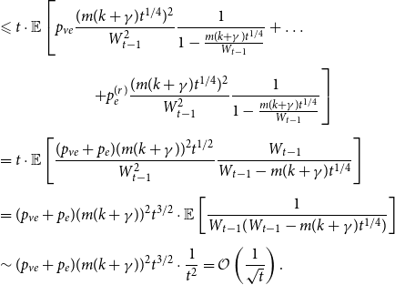 \begin{align*} \begin{split} & \leqslant t \cdot{\mathbb{E}} \left [p_{ve} \frac{(m(k+\gamma )t^{1/4})^2}{W_{t-1}^2}\frac{1}{1-\frac{m(k+\gamma )t^{1/4}}{W_{t-1}}} + \ldots \right . \\[5pt] & \left . \quad \quad \quad \quad \quad \quad + p_{e}^{(r)} \frac{(m(k+\gamma )t^{1/4})^2}{W_{t-1}^2}\frac{1}{1-\frac{m(k+\gamma )t^{1/4}}{W_{t-1}}}\right ] \\[5pt] & = t \cdot{\mathbb{E}} \left [\frac{(p_{ve}+p_e)(m(k+\gamma ))^2 t^{1/2}}{W_{t-1}^2}\frac{W_{t-1}}{W_{t-1}-m(k+\gamma )t^{1/4}} \right ] \\[5pt] & = (p_{ve}+p_e)(m(k+\gamma ))^2 t^{3/2} \cdot{\mathbb{E}}\left [\frac{1}{W_{t-1}(W_{t-1}-m(k+\gamma )t^{1/4})}\right ] \\[5pt] & \sim (p_{ve}+p_e)(m(k+\gamma ))^2 t^{3/2} \cdot \frac{1}{t^2} = \mathcal{O}\left (\frac{1}{\sqrt{t}}\right ). \end{split} \end{align*}
Plugging 9, 10 and 11 into master equation (5) and (6), we obtain
 \begin{align} {\mathbb{E}}[N_{0,t}] ={\mathbb{E}}[N_{0,t-1}] \left (1 - \frac{\gamma (\bar{D}-m p_{ve})}{t(\bar{D}+\gamma \bar{V}) + \mathcal{O}(t^{3/4}\sqrt{\ln{t}})} \right ) + p_v + \mathcal{O}\left (\frac{1}{\sqrt{t}}\right ) \end{align}
and
 \begin{align} \begin{split}{\mathbb{E}}[N_{k,t}] & ={\mathbb{E}}[N_{k,t-1}] \left (1 - \frac{(k+\gamma ) (\bar{D}-mp_{ve})}{t(\bar{D} + \gamma \bar{V})+\mathcal{O}(t^{3/4}\sqrt{\ln{t}})}\right )\\[5pt] & \quad +{\mathbb{E}}[N_{k-1,t-1}] \left (\frac{(k-1+\gamma ) (\bar{D}-mp_{ve})}{t(\bar{D} + \gamma \bar{V})+\mathcal{O}(t^{3/4}\sqrt{\ln{t}})}\right ) + \delta _{k,m}p_{ve} + \mathcal{O}\left (\frac{1}{\sqrt{t}}\right ). \end{split} \end{align}
For  $k \geq 0$ by
  $L_k$ denote the limit
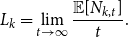 \begin{align*} L_k = \lim _{t \rightarrow \infty } \frac{{\mathbb{E}}[N_{k,t}]}{t}. \end{align*}
First we prove that the limit  $L_0$ exists. We apply Lemma 8 to equation (12) by setting
 \begin{align*} b_t = \frac{\gamma (\bar{D}-m p_{ve})}{\bar{D}+\gamma \bar{V} + \mathcal{O}(t^{3/4}\sqrt{\ln{t}}/t)} \quad \text{and} \quad c_t = p_v + \mathcal{O}\left (\frac{1}{\sqrt{t}}\right ). \end{align*}
We get
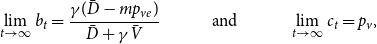 \begin{align*} \lim _{t \rightarrow \infty } b_t = \frac{\gamma (\bar{D}-m p_{ve})}{\bar{D}+\gamma \bar{V}} \quad \quad \quad \text{and} \quad \quad \quad \lim _{t \rightarrow \infty } c_t = p_v, \end{align*}
therefore
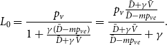 \begin{align*} L_0 = \frac{p_v}{1+\frac{\gamma (\bar{D}-m p_{ve})}{\bar{D}+\gamma \bar{V}}} = \frac{p_v \frac{\bar{D}+\gamma \bar{V}}{\bar{D}-m p_{ve}}}{\frac{\bar{D}+\gamma \bar{V}}{\bar{D}-m p_{ve}} + \gamma }. \end{align*}
Now, we assume that the limit  $L_{k-1}$ exists, and we will show by induction on
  $k$ that
  $L_k$ exists. Again, applying Lemma 8 to equation (13) with
 \begin{align*} b_t = \frac{(k+\gamma ) (\bar{D}-m p_{ve})}{\bar{D}+\gamma \bar{V} + \mathcal{O}(t^{3/4}\sqrt{\ln{t}}/t)} \end{align*}
and
 \begin{align*} c_t = \frac{{\mathbb{E}}[N_{k-1,t-1}]}{t} \left (\frac{(k-1+\gamma ) (\bar{D}-m p_{ve})}{\bar{D}+\gamma \bar{V} + \mathcal{O}(t^{3/4}\sqrt{\ln{t}}/t)}\right ) + \delta _{k,m}p_{ve} +{\mathcal{O}}\left (\frac{1}{\sqrt{t}}\right ) \end{align*}
we get
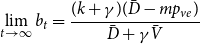 \begin{align*} \lim _{t \rightarrow \infty } b_t = \frac{(k+\gamma ) (\bar{D}-m p_{ve})}{\bar{D}+\gamma \bar{V}} \end{align*}
and
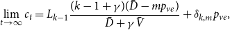 \begin{align*} \lim _{t \rightarrow \infty } c_t = L_{k-1} \frac{(k-1+\gamma ) (\bar{D}-m p_{ve})}{\bar{D}+\gamma \bar{V}} + \delta _{k,m}p_{ve}, \end{align*}
therefore
 \begin{align} L_k = \frac{L_{k-1} \frac{(k-1+\gamma ) (\bar{D}-m p_{ve})}{\bar{D}+\gamma \bar{V}} + \delta _{k,m}p_{ve}}{1+\frac{(k+\gamma ) (\bar{D}-m p_{ve})}{\bar{D}+\gamma \bar{V}}} = \frac{L_{k-1}(k-1+\gamma )+ \delta _{k,m}p_{ve}\frac{\bar{D}+\gamma \bar{V}}{\bar{D}-m p_{ve}}}{k+\gamma +\frac{\bar{D}+\gamma \bar{V}}{\bar{D}-m p_{ve}}}. \end{align}
From now on, for simplicity of notation, we put  $D = \frac{\bar{D}+\gamma \bar{V}}{\bar{D}-m p_{ve}}$; thus, we have
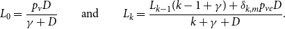 \begin{align*} L_0 = \frac{p_v D}{\gamma + D} \quad \quad \text{and} \quad \quad L_k = \frac{L_{k-1}(k-1+\gamma )+ \delta _{k,m}p_{ve}D}{k + \gamma + D}. \end{align*}
When 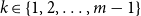 $k \in \{1,2,\ldots,m-1\}$, iterating over
  $k$ gives
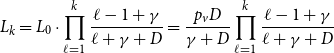 \begin{align*} L_k = L_0 \cdot \prod _{\ell =1}^{k} \frac{\ell -1+\gamma }{\ell +\gamma +D} = \frac{p_v D}{\gamma +D} \prod _{\ell =1}^{k} \frac{\ell -1+\gamma }{\ell +\gamma +D} \end{align*}
and when  $k \geqslant m$
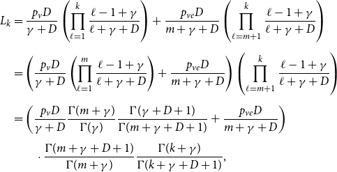 \begin{align*} \begin{split} L_k & = \frac{p_v D}{\gamma +D} \left ( \prod _{\ell =1}^{k} \frac{\ell -1+\gamma }{\ell +\gamma +D} \right ) + \frac{p_{ve} D}{m + \gamma + D} \left ( \prod _{\ell =m+1}^{k} \frac{\ell -1+\gamma }{\ell +\gamma +D} \right )\\[5pt] & = \left (\frac{p_v D}{\gamma +D} \left ( \prod _{\ell =1}^{m} \frac{\ell -1+\gamma }{\ell +\gamma +D}\right ) + \frac{p_{ve}D}{m + \gamma + D} \right ) \left ( \prod _{\ell =m+1}^{k} \frac{\ell -1+\gamma }{\ell +\gamma +D} \right )\\[5pt] & = \left (\frac{p_v D}{\gamma +D} \frac{\Gamma (m+\gamma )}{\Gamma (\gamma )}\frac{\Gamma (\gamma + D +1)}{\Gamma (m+\gamma +D+1)} +\frac{p_{ve}D}{m + \gamma + D}\right ) \\[5pt] & \quad \quad \cdot \frac{\Gamma (m+\gamma +D+1)}{\Gamma (m+\gamma )}\frac{\Gamma (k+\gamma )}{\Gamma (k+\gamma +D+1)}, \end{split} \end{align*}
where  $\Gamma (x)$ is the gamma function. Since
 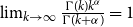 $\lim _{k \rightarrow \infty } \frac{\Gamma (k)k^{\alpha }}{\Gamma (k+\alpha )} = 1$ for constant
  $\alpha \in \mathbb{R}$, we get
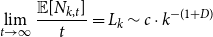 \begin{align*} \lim _{t \rightarrow \infty } \frac{{\mathbb{E}}[N_{k,t}]}{t} = L_k \sim c \cdot k^{-(1+D)} \end{align*}
(“ $\sim$” refers to the limit by
  $k \rightarrow \infty$) for
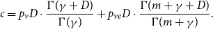 \begin{align*} c = p_v D\cdot \frac{\Gamma (\gamma +D)}{\Gamma (\gamma )} + p_{ve} D\cdot \frac{\Gamma (m+\gamma +D)}{\Gamma (m+\gamma )}. \end{align*}
Hence, by Lemma 1, we obtain
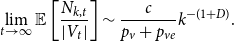 \begin{align*} \lim _{t \rightarrow \infty }{\mathbb{E}}\left [\frac{N_{k,t}}{|V_t|}\right ] \sim \frac{c}{p_v+p_{ve}} k^{-(1+D)}. \end{align*}
We infer that the degree distribution of our hypergraph follows a power-law with
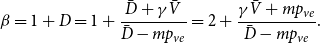 \begin{align*} \beta = 1+D = 1+\frac{\bar{D}+\gamma \bar{V}}{\bar{D}-m p_{ve}} = 2 + \frac{\gamma \bar{V} + m p_{ve}}{\bar{D} - m p_{ve}}. \end{align*}
B. Modularity of $\mathbf{G(G_0,p,M,X,P,\gamma )}$

Proof of Lemma 4. Let  $\mathcal{C} = \{C^{(1)}, C^{(2)}, \ldots, C^{(r)}\}$ and for
  $i \in \{1,2,\ldots,r\}$ let
  $\tilde{s}_i$ be the probability that a randomly chosen hyperedge joins at least two communities and
  $C^{(i)}$ is one of them. Note that for
  $s_i$ defined as in Lemma 3 (i.e. the probability that a randomly chosen hyperedge has at least one vertex in
  $C^{(i)}$) we get
  $s_i = \tilde{s}_i + p_i$. By Lemma 3, we get that with high probability
 \begin{align} \begin{split} \lim _{t \rightarrow \infty } q^*(G) & \geqslant (1+o(1)) \left ( \sum _{i=1}^{r} p_i - \sum _{i=1}^{r} \sum _{\ell \geqslant 1} a_{\ell }\left (\frac{(z-1)\tilde{s}_i+zp_i}{\delta }\right )^{\ell } \right )\\[5pt] & = (1+o(1)) \left ( (1-\alpha ) - \sum _{\ell \geqslant 1} \frac{a_{\ell }}{\delta ^{\ell }} \sum _{i=1}^{r} ((z-1)\tilde{s}_i+zp_i)^{\ell } \right ) \\[5pt] & = (1+o(1)) \cdot \\[5pt] & \cdot \left ((1-\alpha ) - \frac{a_1}{\delta }\left ((z-1) \sum _{i=1}^{r} \tilde{s}_i + z \sum _{i=1}^{r} p_i \right ) - \sum _{\ell \geqslant 2} \frac{a_{\ell }}{\delta ^{\ell }} \sum _{i=1}^{r} ((z-1)\tilde{s}_i+zp_i)^{\ell }\right ). \end{split} \end{align}
Now, by  $r_k$ denote the probability that a randomly chosen hyperedge joins exactly
  $k$ communities. Note that
 \begin{align} \sum _{i=1}^{r} \tilde{s}_i = 2r_2 + 3r_3 + \ldots + zr_z \leqslant z(1 - \sum _{i=1}^{r} p_i) = z \alpha . \end{align}
Thus,
 \begin{align} \frac{a_1}{\delta }\left ((z-1) \sum _{i=1}^{r} \tilde{s}_i + z \sum _{i=1}^{r} p_i \right ) \leqslant \frac{a_1}{\delta }\left ((z-1) z \alpha + z (1-\alpha ) \right ) = a_1 \left (\frac{z}{\delta }\right )((z-2)\alpha +1). \end{align}
Moreover,
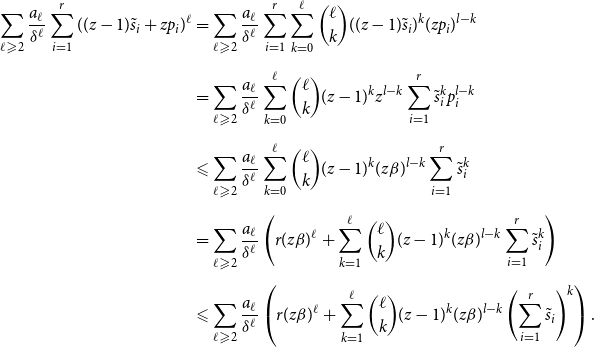 \begin{align*} \sum _{\ell \geqslant 2} \frac{a_{\ell }}{\delta ^{\ell }} \sum _{i=1}^{r} ((z-1)\tilde{s}_i +zp_i)^{\ell } & = \sum _{\ell \geqslant 2} \frac{a_{\ell }}{\delta ^{\ell }} \sum _{i=1}^{r} \sum _{k=0}^{\ell }\substack{\ell \\ k}((z-1)\tilde{s}_i)^k (zp_i)^{l-k} \\[5pt] & = \sum _{\ell \geqslant 2} \frac{a_{\ell }}{\delta ^{\ell }} \sum _{k=0}^{\ell }\substack{\ell \\ k}(z-1)^{k} z^{l-k} \sum _{i=1}^{r} \tilde{s}_i^k p_i^{l-k} \\[5pt] & \leqslant \sum _{\ell \geqslant 2} \frac{a_{\ell }}{\delta ^{\ell }} \sum _{k=0}^{\ell }\substack{\ell \\ k}(z-1)^{k} (z\beta )^{l-k} \sum _{i=1}^{r} \tilde{s}_i^k \\[5pt] & = \sum _{\ell \geqslant 2} \frac{a_{\ell }}{\delta ^{\ell }} \left ( r (z \beta )^{\ell } + \sum _{k=1}^{\ell }\substack{\ell \\ k}(z-1)^{k} (z\beta )^{l-k} \sum _{i=1}^{r} \tilde{s}_i^k \right ) \\[5pt] & \leqslant \sum _{\ell \geqslant 2} \frac{a_{\ell }}{\delta ^{\ell }} \left ( r (z \beta )^{\ell } + \sum _{k=1}^{\ell }\substack{\ell \\ k}(z-1)^{k} (z\beta )^{l-k} \left (\sum _{i=1}^{r} \tilde{s}_i\right )^k \right ). \end{align*}
Next, by (16) we get
 \begin{align} \begin{split} \sum _{\ell \geqslant 2} \frac{a_{\ell }}{\delta ^{\ell }} \sum _{i=1}^{r} ((z-1)\tilde{s}_i +zp_i)^{\ell } & \leqslant \sum _{\ell \geqslant 2} \frac{a_{\ell }}{\delta ^{\ell }} \left ( r (z \beta )^{\ell } + \sum _{k=1}^{\ell }\substack{\ell \\ k}(z-1)^{k} (z\beta )^{l-k} (z \alpha )^k \right ) \\[5pt] & = \sum _{\ell \geqslant 2} \frac{a_{\ell }}{\delta ^{\ell }} \left ( (r-1) (z \beta )^{\ell } + \sum _{k=0}^{\ell }\substack{\ell \\ k}((z-1)z \alpha )^{k} (z\beta )^{l-k} \right ) \\[5pt] & = \sum _{\ell \geqslant 2} \frac{a_{\ell }}{\delta ^{\ell }} \left ( (r-1) (z \beta )^{\ell } + ((z-1)z \alpha + z \beta )^{\ell } \right ) \\[5pt] & = \sum _{\ell \geqslant 2} a_{\ell }\left (\frac{z}{\delta }\right )^{\ell }\left ((r-1)\beta ^{\ell } + ((z-1)\alpha + \beta )^{\ell }\right ). \end{split} \end{align}
Finally, plugging (17) and (18) into (15) we get that with high probability
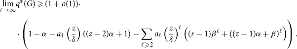 \begin{align*} \begin{split} \lim _{t \rightarrow \infty } & q^*(G) \geqslant (1+o(1)) \cdot \\[5pt] & \cdot \left (1-\alpha - a_1 \left (\frac{z}{\delta }\right )((z-2)\alpha +1) - \sum _{\ell \geqslant 2} a_{\ell }\left (\frac{z}{\delta }\right )^{\ell }\left ((r-1)\beta ^{\ell } + ((z-1)\alpha + \beta )^{\ell }\right ) \right ). \end{split} \end{align*}


 Open access