


1. Introduction
For homogeneous isotropic turbulence, the energy spectrum, which is the Fourier transform of the two-point velocity correlation, is frequently used to describe the scale dependence of turbulent fluctuations. The energy transfer, such as a cascade from low to high wavenumbers, has been studied in detail, and several closure theories have been developed (Frisch Reference Frisch1995). In contrast, one-point statistical quantities are mainly employed for inhomogeneous turbulence, such as the turbulent kinetic energy. The energy production, dissipation and transfer in the physical space are described and predicted using one-point closure models (Pope Reference Pope2000). The treatment of two-point quantities in inhomogeneous turbulence models is a highly complex process, although the scale dependence of the energy is important for understanding and predicting turbulent flows.
To improve the turbulence models, attempts have been made to use the energy spectrum for inhomogeneous turbulence. The two-scale turbulence theory defines the fast and slow variables for space coordinates (Yoshizawa Reference Yoshizawa1984, Reference Yoshizawa1998). The Fourier transform of a velocity field with respect to the fast variable was performed to use the closure theory for homogeneous isotropic turbulence (Kraichnan Reference Kraichnan1971; Leslie Reference Leslie1973), whereas the dependence of the velocity on the slow variable was used to describe the inhomogeneity of the turbulent field. In the turbulence model developed by Schiestel (Reference Schiestel1987), multi-scale turbulent kinetic energies were introduced by dividing the energy spectrum into several wavenumber parts. The transport equations for the kinetic energies at different scales were used to improve the prediction of turbulent flow (Chaouat & Schiestel Reference Chaouat and Schiestel2005; Schiestel & Dejoan Reference Schiestel and Dejoan2005). In these studies, the energy transfer between different scales was used to improve the turbulence models, while the Fourier transform and energy spectrum were introduced in an approximate manner; hence, the procedures must be justified physically.
Instead of the energy spectrum, the second-order structure function  $\langle \delta u_i^2({\boldsymbol {x}},{\boldsymbol {r}})\rangle$ (where $\delta {u_i}({\boldsymbol {x}},{\boldsymbol {r}}) = {u_i}({\boldsymbol {x}} + {\boldsymbol {r}}) - {u_i}({\boldsymbol {x}})$ and ${u_i}({\boldsymbol {x}})$ is the velocity fluctuation) and the two-point velocity correlation ${Q_{ii}}({\boldsymbol {x}},{\boldsymbol {r}})$ ( ${=} \langle {u_i}({\boldsymbol {x}}){u_i}({\boldsymbol {x}} + {\boldsymbol {r}})\rangle$) in the physical space can be used to describe the kinetic energy at the length scale of $r$ (
$r$ ( ${=}|{\boldsymbol {r}}|$). For homogeneous isotropic turbulence, the Kármán–Howarth equation and Kolmogorov equation were formulated using the two-point correlation and structure function, respectively (Frisch Reference Frisch1995). Several attempts have been made to extend these equations to inhomogeneous turbulence (Danaila et al. Reference Danaila, Anselmet, Zhou and Antonia2001; Hill Reference Hill2002; Davidson Reference Davidson2004; Marati, Casciola & Piva Reference Marati, Casciola and Piva2004; Danaila et al. Reference Danaila, Krawczynski, Thiesset and Renou2012; Cimarelli, De Angelis & Casciola Reference Cimarelli, De Angelis and Casciola2013; Hamba Reference Hamba2015; Cimarelli et al. Reference Cimarelli, De Angelis, Jiménez and Casciola2016; Hamba Reference Hamba2018; Mollicone et al. Reference Mollicone, Battista, Gualtieri and Casciola2018; Arun et al. Reference Arun, Sameen, Srinivasan and Girimaji2021). Danaila et al. (Reference Danaila, Anselmet, Zhou and Antonia2001) examined the turbulent diffusion and dissipation terms at the centre of a channel flow and proposed a generalised form of the Kolmogorov equation. Hill (Reference Hill2002) theoretically derived the exact transport equation for the structure function in inhomogeneous turbulence and discussed its potential applications. Marati et al. (Reference Marati, Casciola and Piva2004) evaluated the structure function equation using the direct numerical simulation (DNS) data of a turbulent channel flow. Cimarelli et al. (Reference Cimarelli, De Angelis and Casciola2013) and Cimarelli et al. (Reference Cimarelli, De Angelis, Jiménez and Casciola2016) examined the energy flux occurring in the scale space and physical space in turbulent channel flows. Danaila et al. (Reference Danaila, Krawczynski, Thiesset and Renou2012) developed a scale-by-scale kinetic energy budget equation using the structure function and examined experimental data obtained from a multiple-opposed jet flow. Using the generalised Kolmogorov equation, Mollicone et al. (Reference Mollicone, Battista, Gualtieri and Casciola2018) described the scale-by-scale turbulence dynamics in a separation bubble generated by a bulge in a turbulent channel flow. Davidson (Reference Davidson2004) defined the turbulent energy density in the scale space using the $r$ derivative of the structure function, and compared the energy density in homogeneous isotropic turbulence and wall turbulence (Davidson & Pearson Reference Davidson and Pearson2005; Davidson, Nickels & Krogstad Reference Davidson, Nickels and Krogstad2006). Using the two-point velocity correlation, Hamba (Reference Hamba2015) proposed an expression for the energy density in the scale space and examined the energy transfer in a turbulent channel flow. Arun et al. (Reference Arun, Sameen, Srinivasan and Girimaji2021) derived the scale-space energy density equation for compressible flows and investigated the effects of variable density and dilatation on an energy cascade in compressible mixing layers.
In addition to two-point statistical quantities, the low-pass filtering operation of a velocity field is also an effective tool for examining scale-by-scale turbulent fluctuations. Using the generalised Kolmogorov equation for a filtered velocity field, Cimarelli & De Angelis (Reference Cimarelli and De Angelis2012) examined the scale-by-scale budget of the turbulent energy near the wall of a turbulent channel flow. Applying a Gaussian filter to the DNS velocity field, Motoori & Goto (Reference Motoori and Goto2019) investigated the generation mechanism of the hierarchy of vortices in a turbulent boundary layer. Using a local volume average, Watanabe, da Silva & Nagata (Reference Watanabe, da Silva and Nagata2020) analysed the sub-grid scale energy budget near the turbulent/non-turbulent interfacial layer. The wavelet transform of a velocity field is also considered a band-pass filtered velocity, which has been widely used to analyse and simulate coherent structures of turbulence (Farge Reference Farge1992; Schneider & Vasilyev Reference Schneider and Vasilyev2010). However, its application in turbulence theory is limited. Altaisky, Hnatich & Kaputkina (Reference Altaisky, Hnatich and Kaputkina2018) combined the wavelet transform with the renormalisation group theory (Yahkot & Orszag Reference Yahkot and Orszag1986) to study the statistics at different scales.
Similar to the energy spectrum, the energy density in the scale space should satisfy the following conditions (Davidson Reference Davidson2004). First, the integral of the energy density over all scales should be equal to the turbulent kinetic energy. Second, the energy density should be non-negative. For example, the structure function is non-negative but its integral is not equal to the turbulent kinetic energy. Instead, the structure function itself tends to be twice the energy as  $r \to \infty$. In contrast, Davidson (Reference Davidson2004) introduced the gradient of the structure function as the energy density, which satisfies the first property but is not non-negative. The same holds true for the energy density based on the two-point velocity correlation proposed by Hamba (Reference Hamba2015). By integrating the velocity correlation with a filter function, Hamba (Reference Hamba2018) improved the energy density so that it is non-negative for homogeneous turbulence. Nonetheless, it fails to satisfy the non-negative property for inhomogeneous turbulence. It shows a small negative value in the region very close to the wall in a turbulent channel flow. In the present study, we use filtered velocities in a systematic manner to propose a new expression for the energy density in the scale space to clarify the reasons for the negative values of the energy density. The new expression consists of homogeneous and inhomogeneous parts. The former is expressed in terms of the variance of the filtered velocity and is always non-negative, whereas the latter can be negative because of the turbulence inhomogeneity. Using the new expression, we investigate the effects of the inhomogeneity on the negative values of the energy density. The scale-space energy density based on filtered velocities will be useful in describing the turbulence statistics at different scales and to obtain a better understanding of inhomogeneous turbulence.
This paper is organised as follows. In § 2, we introduce three filtered velocities and propose a new expression for the energy density in the scale space. In § 3, we evaluate the energy density using the DNS data of homogeneous isotropic turbulence, and compare the results between the cases of one- and three-dimensional filtering. In § 4, we evaluate the homogeneous and inhomogeneous parts of the energy density using the DNS data of a turbulent channel flow. We examine how the profile of the turbulent energy near the wall affects the inhomogeneous part and induces a negative value of the energy density. Finally, we conclude the paper in § 5.
2. Turbulent energy density in scale space
2.1. Energy spectrum and scale-space energy density
To compare the scale-space energy density with the energy spectrum, we first describe the energy spectrum, which is also an energy density treated in the wavenumber space. The velocity is divided into the mean and fluctuating parts as follows:
 \begin{equation} u_i^*({\boldsymbol{x}}) = {U_i}({\boldsymbol{x}}) + {u_i}({\boldsymbol{x}}),\quad {U_i} = \langle u_i^*\rangle , \end{equation}
where  $\langle \ \rangle$ denotes the ensemble average. For homogeneous turbulence, the velocity fluctuation ${u_i}({\boldsymbol {x}})$ is often expressed in terms of its Fourier transform ${u_i}({\boldsymbol {k}})$ as follows:
 \begin{equation} {u_i}({\boldsymbol{x}}) = \int {\mathrm{d}{\boldsymbol{k}}}\, {u_i}({\boldsymbol{k}})\exp (\mathrm{i}{\boldsymbol{k}} \boldsymbol{\cdot} {\boldsymbol{x}}),\quad \int {\mathrm{d}{\boldsymbol{k}}} = \int_{ - \infty }^\infty {\mathrm{d}{k_x}} \int_{ - \infty }^\infty {\mathrm{d}{k_y}} \int_{ - \infty }^\infty {\mathrm{d}{k_z}} . \end{equation}
This expression indicates that the velocity fluctuations in the physical space can be decomposed into Fourier modes in the wavenumber space. The velocity variance  $\langle {u_i}({\boldsymbol {x}}){u_i}({\boldsymbol {x}})\rangle$ can also be decomposed in the wavenumber space as
 \begin{equation} \langle {u_i}({\boldsymbol{x}}){u_i}({\boldsymbol{x}})\rangle = \int {\mathrm{d}{\boldsymbol{k}}} \,{Q_{ii}}({\boldsymbol{k}}) , \end{equation}
where  ${Q_{ii}}({\boldsymbol {k}})$ is the Fourier transform of ${Q_{ii}}({\boldsymbol {x}},{\boldsymbol {r}})$ with respect to ${\boldsymbol {r}}$ and the summation convention is used for repeated indices. The Fourier transform ${Q_{ii}}({\boldsymbol {k}})$ is related to the velocity fluctuation ${u_i}({\boldsymbol {k}})$ as follows:
 \begin{equation} \langle {u_i}({\boldsymbol{k}})u_i^{\dagger} ({\boldsymbol{k}})\rangle = {Q_{ii}}({\boldsymbol{k}})\delta ({\boldsymbol{0}}) , \end{equation}
where  $^{\dagger}$ denotes the complex conjugate and $\delta ({\boldsymbol {0}})$ is the Dirac delta function $\delta ({\boldsymbol {k}})$ with ${\boldsymbol {k}} = {\boldsymbol {0}}$. For homogeneous isotropic turbulence, the energy spectrum $E(k)$ ( ${=}2{\rm \pi} {k^2}{Q_{ii}}({\boldsymbol {k}})$) is often introduced. The energy spectrum $E(k)$ represents the energy density in the wavenumber space and satisfies the following properties:
 \begin{gather} K = \int_0^\infty {\mathrm{d}k}\, E(k) , \end{gather}
 \begin{gather}E(k) \geqslant 0 , \end{gather}
where  $K$ (
$K$ ( ${=}\langle u^{2}_{i}\rangle /2$) is the turbulent kinetic energy. The energy spectrum $E(k)$ contains information on the turbulence intensity and the scale dependence of the turbulent fluctuations; it is considered as the kinetic energy of eddies of size ${\rm \pi} /k$. Because the energy spectrum $E(k)$ is directly related to the velocity fluctuation ${u_i}({\boldsymbol {k}})$ through the relationship in (2.4), it is clearly non-negative. On the basis of the governing equation for ${u_i}({\boldsymbol {k}})$, the transport equation for the energy spectrum was analysed and modelled in statistical theories for homogeneous isotropic turbulence. The decomposition of the instantaneous velocity given by (2.2a,b) and that of the turbulent energy given by (2.5) and (2.6) are very useful expressions in analysing turbulent statistics and developing closure theories for homogeneous turbulence. We will try to determine the corresponding expressions for inhomogeneous turbulence.
Instead of the energy spectrum in the wavenumber space, the energy density in the scale space can be used for the inhomogeneous turbulence. The energy density  $E({\boldsymbol {x}},r)$ in the scale space is a function of both position ${\boldsymbol {x}}$ and length scale $r$, and should satisfy the following properties:
 \begin{gather} K({\boldsymbol{x}}) = \int_0^\infty {\mathrm{d}r} \,E({\boldsymbol{x}},r) , \end{gather}
 \begin{gather}E({\boldsymbol{x}},r) \geqslant 0 , \end{gather}
as in the cases of (2.5) and (2.6) for the energy spectrum (Davidson Reference Davidson2004). Although several energy densities and scale energies have been proposed, there is still no quantity that satisfies both properties. For example, Hill (Reference Hill2002) derived the transport equation for the second-order structure function. The structure function satisfies (2.8) but not (2.7); that is, it is non-negative but its integral is not equal to the turbulent kinetic energy. Davidson (Reference Davidson2004) proposed the energy density using the following structure function:
 \begin{equation} E({\boldsymbol{x}},r) ={-} \frac{3}{8}{r^2}\frac{\partial }{{\partial r}}\frac{1}{r}\frac{\partial }{{\partial r}}\langle {(\Delta u)^2}\rangle , \end{equation}
where  $\Delta u = {u_x}({\boldsymbol {x}} + r{{\boldsymbol {e}}_x}) - {u_x}({\boldsymbol {x}})$. Conversely, it satisfies (2.7) but not (2.8). The same holds true for the energy density proposed by Hamba (Reference Hamba2015) using the two-point velocity correlation as follows:
 \begin{equation} E({\boldsymbol{x}},r) ={-} \frac{\partial }{{\partial r}}{E_ > }({\boldsymbol{x}},r) , \end{equation}
where  ${E_ > }({\boldsymbol {x}},r) = {Q_{ii}}({\boldsymbol {x}},r{{\boldsymbol {e}}_r})/2$. Here, ${E_ > }({\boldsymbol {x}},r)$ represents the kinetic energy of eddies with sizes equal to or greater than $r$. In (2.9) and (2.10), the derivative with respect to $r$ is introduced so that $E({\boldsymbol {x}},r)$ can satisfy (2.7); however, they are not necessarily non-negative. Hamba (Reference Hamba2018) improved the energy density by introducing a filter function $G(\xi,r)$ as follows:
 \begin{equation} {E_ > }({\boldsymbol{x}},r) = \int_{ - \infty }^\infty {\mathrm{d}\xi } \frac{1}{2}{Q_{ii}}({\boldsymbol{x}},\xi )G(\xi ,r) ,\quad G(\xi ,r) = \frac{1}{{\sqrt {2{\rm \pi} } r}}\exp \left( { - \frac{{{\xi ^2}}}{{2{r^2}}}} \right) . \end{equation}
Here, the filtered correlation is used for  ${E_ > }({\boldsymbol {x}},r)$ instead of the correlation ${Q_{ii}}({\boldsymbol {x}},{\boldsymbol {r}})$ itself. As a result, the energy density is always non-negative for homogeneous turbulence. However, it fails to satisfy the non-negative property for inhomogeneous turbulence; it shows a small negative value in the region very close to the wall in a turbulent channel flow (Hamba Reference Hamba2018).
Compared with the energy density, the second-order structure function  $\langle \delta u_i^2({\boldsymbol {x}},{\boldsymbol {r}})\rangle$ has a well-defined theoretical background and physical meaning. It is non-negative and represents the kinetic energy of eddies with sizes equal to or less than $r$. However, the problem arises when we consider its behaviour as $r \to \infty$ in turbulent flows inhomogeneous in all directions. When $r$ is much greater than the integral length scale, we have $\langle \delta u_i^2({\boldsymbol {x}},{\boldsymbol {r}})\rangle \simeq \langle u^{2}_{i}({\boldsymbol {x}}+{\boldsymbol {r}})\rangle + \langle u^{2}_{i}({\boldsymbol {x}})\rangle$, which is the sum of the kinetic energies at two positions apart from each other in an inhomogeneous direction. The energy density is expected to be used not only for the analysis of turbulent statistics but also for turbulence modelling where the kinetic energy at a single position should be decomposed into several scales. This is why we treat the energy density that satisfies (2.7) rather than the second-order structure function.
2.2. Filtered velocities
In this study, instead of the filtered correlation given by (2.11a,b), we start from filtered velocities to derive an expression for the energy density in the scale space. For simplicity, we describe the formulation in the case of one-dimensional filtering. We introduce three filtered velocities using different filter functions. The first filtered velocity  ${\bar {u}}_{i}(x,s)$ is an ordinary one with a Gaussian function that is widely used in large eddy simulation (LES). It is defined as
 \begin{equation} {\bar{u}_i}(x,s) = \bar{F}(s)*{u_i}(x) = \int_{ - \infty }^\infty {\mathrm{d} x'}\,\bar{G}(x - x',s){u_i}(x') , \end{equation}
where  $\bar {G}(x-x',s)$ is the filter function given by
 \begin{equation} \bar{G}(x - x',s) = \frac{1}{{{{(2{\rm \pi} s)}^{1/2}}}}\exp \left[ { - \frac{{{{(x - x')}^2}}}{{2s}}} \right] . \end{equation}
It should be noted that instead of the length scale  $r$, we adopt a quantity $s$ with a dimension of the square of the length in (2.12) and (2.13). Compared with the filtered velocity with $r$, this choice simplifies the formulation; for example, double filtering is expressed in terms of the addition of $s$ as $\bar {F}({s_1})*\bar {F}({s_2})*{u_i} = \bar {F}({s_1} + {s_2})*{u_i}$. Moreover, it yields a simple relationship between the derivatives with respect to $s$ and $x$, as will be discussed later. Hereafter, we refer to $s$ as the scale. The filtered velocity ${\bar {u}_i}(x,s)$ represents the velocity with a scale equal to or greater than $s$. It corresponds to the resolved (grid-scale) velocity in the LES. The profile of $\bar {G}(x,s)$ as a function of $x$ for $s = 1$ is shown in figure 1. When $s = 0$, the filtered velocity is reduced to the original velocity as ${\bar {u}_i}(x,0) = {u_i}(x)$ because $\bar {G}(x - x',0) = \delta (x - x')$.


By differentiating  ${\bar {u}_i}(x,s)$ with respect to $s$, we can obtain a filtered velocity with a scale equal to $s$. We define the second filtered velocity ${\hat {u}_i}(x,s)$ as follows:
 \begin{equation} {\hat{u}_i}(x,s) \equiv{-} \frac{\partial }{{\partial s}}{\bar{u}_i}(x,s) = \hat{F}(s)*{u_i}(x) = \int_{ - \infty }^\infty {\mathrm{d} x'}\,\hat{G}(x - x',s){u_i}(x') , \end{equation}
where
 \begin{align} \hat{G}(x - x',s) \equiv{-} \frac{\partial }{{\partial s}}\bar{G}(x - x',s) = \frac{1}{{{{(2{\rm \pi} s)}^{1/2}}}}\left[ {\frac{1}{{2s}} - \frac{{{{(x - x')}^2}}}{{2{s^2}}}} \right]\exp \left[ { - \frac{{{{(x - x')}^2}}}{{2s}}} \right] . \end{align}
The profile of  $\hat {G}(x,s)$ for $s = 1$ is also plotted in figure 1; it is an even function of $x$, as in the case of $\bar {G}(x,s)$. The filtered velocity ${\bar {u}_i}(x,s)$ and the original velocity ${u_i}(x)$ can be written in terms of ${\hat {u}_i}(x,s)$ as
 \begin{gather} {\bar{u}_i}(x,s) = \int_s^\infty {\mathrm{d}s'} \,{\hat{u}_i}(x,s') , \end{gather}
 \begin{gather}{u_i}(x) = \int_0^\infty {\mathrm{d}s} \,{\hat{u}_i}(x,s) , \end{gather}
respectively, where it is assumed that  ${\bar {u}_i}(x,\infty ) = 0$. Equation (2.17) indicates that the velocity ${u_i}(x)$ is decomposed into the modes ${\hat {u}_i}(x,s)$ in the scale space and corresponds to the Fourier transform given by (2.2a,b). Because we adopted a Gaussian filter function in (2.13), we have the following relationships between the derivatives with respect to $s$ and $x$:
$x$:
 \begin{equation} \frac{\partial }{{\partial s}}\bar{G}(x - x',s) = \frac{1}{2}\frac{{{\partial ^2}}}{{\partial {x^2}}}\bar{G}(x - x',s) ,\quad \frac{\partial }{{\partial s}}\bar{u}_{i}(x,s) = \frac{1}{2}\frac{{{\partial ^2}}}{{\partial {x^2}}}{\bar{u}_i}(x,s) , \end{equation}
which lead to
 \begin{equation} \hat{G}(x - x',s) ={-} \frac{1}{2}\frac{{{\partial ^2}}}{{\partial {x^2}}}\bar{G}(x - x',s) ,\quad \hat{u}_{i}(x,s) ={-} \frac{1}{2}\frac{{{\partial ^2}}}{{\partial {x^2}}}{\bar{u}_i}(x,s) . \end{equation}
The filtered velocity  ${\hat {u}_i}(x,s)$ can also be obtained from the second $x$ derivative of ${\bar {u}_i}(x,s)$ instead of the $s$ derivative. The relationships given by (2.18a,b) can be interpreted as the diffusion equations for $\bar {G}(x - x',s)$ and ${\bar {u}_i}(x,s)$ if we consider the scale $s$ as the time. In general, the profile of the filtered velocity becomes smoother as the scale increases. Such a variation of the profile with increasing scale can be expressed in terms of the time evolution of the solution of the diffusion equation (see Appendix A for details).
As the filtered velocity  ${\hat {u}_i}(x,s)$ is proportional to the second $x$ derivative of ${\bar {u}_i}(x,s)$, we can also introduce the first $x$ derivative of ${\bar {u}_i}(x,s)$. We define the third filtered velocity ${\tilde {u}_i}(x,s)$ as follows:
 \begin{equation} {\tilde{u}_i}(x,s) \equiv \frac{\partial }{{\partial x}}{\bar{u}_i}(x,s) = \tilde{F}(s)*{u_i}(x) = \int_{ - \infty }^\infty {\mathrm{d} x'}\, \tilde{G}(x - x',s){u_i}(x') , \end{equation}
where
 \begin{equation} \tilde{G}(x - x',s) \equiv \frac{\partial }{{\partial x}}\bar{G}(x - x',s) ={-} \frac{1}{{{{(2{\rm \pi} s)}^{1/2}}}}\frac{{x - x'}}{s}\exp \left[ { - \frac{{{{(x - x')}^2}}}{{2s}}} \right] . \end{equation}
The profile of  $\tilde {G}(x,s)$ for $s = 1$ is also plotted in figure 1. It is an odd function of $x$ in contrast to $\bar {G}(x,s)$ and $\hat {G}(x,s)$. This velocity is also considered the filtered velocity with a scale equal to $s$. The original velocity can be expressed in terms of the following integral:
 \begin{equation} {u_i}(x) ={-} \int_0^\infty {\mathrm{d}s} \,\tilde{F}(s)*{\tilde{u}_i}(x,s) ={-} \int_0^\infty {\mathrm{d}s} \int_{ - \infty }^\infty {\mathrm{d} x'} \,\tilde{G}(x - x',s){\tilde{u}_i}(x',s) . \end{equation}
The expression is rather complex compared with (2.17) because additional filtering is necessary to reconstruct the velocity. It should be noted that the filtered velocity  ${\tilde {u}_i}(x,s)$ is a continuous wavelet transform of ${u_i}(x)$ (see Appendix B for details).
We have introduced three filtered velocities. The first filtered velocity  ${\bar {u}}_{i}$ with a Gaussian filter is commonly used in the LES. Another filter function such as a top-hat filter is also possible in the present formulation. The second filtered velocity ${\hat {u}}_{i}$ can be defined by (2.14) and the relationships given by (2.16) and (2.17) also hold for general filter functions. However, the relationships given by (2.18a,b) and (2.19a,b) hold only when the Gaussian filter is used. Because these simple relationships are very useful for later formulation, we adopted the Gaussian filter as a first filtered velocity. With respect to the $x$ derivative, ${\bar {u}}_{i}$ is of the zeroth order and ${\hat {u}}_{i}[=-(1/2)(\partial ^{2}/\partial x^{2}){\bar {u}}_{i}]$ is of the second order. In the next subsection, we will require that $2\langle {\bar {u}}_{i}{\hat {u}}_{i}\rangle \simeq \langle {\tilde {u}}_{i}{\tilde {u}}_{i}\rangle$. This is why we introduced the third filtered velocity ${\tilde {u}}_{i}[{=}(\partial /\partial x){\bar {u}}_{i}]$ which is of the first order.
2.3. New energy density in scale space
In this section, we analyse the variances of the filtered velocities defined in § 2.2 to propose a new expression for the energy density in the scale space. The variance of the original velocity  ${Q_{ii}}(x) = \langle {u_i}(x){u_i}(x)\rangle$ gives the turbulent kinetic energy $K$ (
$K$ ( $= {Q_{ii}}(x)/2$). The variance of the filtered velocity, written as
 \begin{equation} {\bar{Q}_{ii}}(x,s) = \langle {\bar{u}_i}(x,s){\bar{u}_i}(x,s)\rangle , \end{equation}
gives another energy  ${\bar {Q}_{ii}}(x,s)/2$, which represents the kinetic energy of eddies with scales equal to or greater than $s$, such as ${E_ > }({\boldsymbol {x}},r)$ given by (2.11a,b). In fact, ${\bar {Q}_{ii}}(x,s)/2$ is equivalent to ${E_ > }({\boldsymbol {x}},r)$ for homogeneous turbulence (Hamba Reference Hamba2018). When $s = 0$, the variance is reduced to the original turbulent energy as
 \begin{equation} {\bar{Q}_{ii}}(x,0)( = \langle {\bar{u}_i}(x,0){\bar{u}_i}(x,0)\rangle ) = {Q_{ii}}(x) . \end{equation}
By differentiating  ${\bar {Q}_{ii}}(x,s)$ with respect to $s$, we can define the scale-space energy density ${\hat {Q}_{ii}}(x,s)/2$, where
 \begin{equation} {\hat{Q}_{ii}}(x,s) \equiv{-} \frac{\partial }{{\partial s}}{\bar{Q}_{ii}}(x,s) = 2\langle {\hat{u}_i}(x,s){\bar{u}_i}(x,s)\rangle , \end{equation}
as in the case of  $E({\boldsymbol {x}},r)$ given by (2.10). The following relationships are satisfied:
 \begin{equation} \tfrac{1}{2}{\bar{Q}_{ii}}(x,s) = \int_s^\infty {\mathrm{d}s'} \tfrac{1}{2}{\hat{Q}_{ii}}(x,s') ,\quad K(x) = \int_0^\infty {\mathrm{d}s}\tfrac{1}{2} {\hat{Q}_{ii}}(x,s) , \end{equation}
where it is assumed that  ${\bar {Q}_{ii}}(x,\infty ) = 0$. In contrast to ${Q_{ii}}({\boldsymbol {k}})$ in (2.4), ${\hat {Q}_{ii}}(x,s)$ is not given by the variance of ${\hat {u}_i}(x,s)$ but by the correlation between ${\hat {u}_i}(x,s)$ and ${\bar {u}_i}(x,s)$ in (2.25); it is not necessarily non-negative. Therefore, the energy density ${\hat {Q}_{ii}}(x,s)/2$ satisfies (2.7) but not (2.8), as in the case of previous energy densities.
In this study, we investigate the energy density in detail using the third filtered velocity  ${\tilde {u}_i}(x,s)$. The variance of ${\tilde {u}_i}(x,s)$, given by
 \begin{equation} {\tilde{Q}_{ii}}(x,s) = \langle {\tilde{u}_i}(x,s){\tilde{u}_i}(x,s)\rangle , \end{equation}
is non-negative. Using (2.19b) for  ${\hat {u}_i}(x,s)$, we can derive the relationship between ${\hat {Q}_{ii}}(x,s)/2$ and ${\tilde {Q}_{ii}}(x,s)/2$ as follows:
 \begin{equation} \frac{1}{2}{\hat{Q}_{ii}}(x,s) = \frac{1}{2}{\tilde{Q}_{ii}}(x,s) - \frac{1}{4}\frac{{{\partial ^2}}}{{\partial {x^2}}}{\bar{Q}_{ii}}(x,s) . \end{equation}
For homogeneous turbulence, only the first term remains on the right-hand side of (2.28). The second term disappears because it is the second derivative of an averaged quantity. Here, we call the first and second terms the homogeneous and inhomogeneous parts of the energy density, respectively. We can see that the energy density  ${\hat {Q}_{ii}}(x,s)/2$ is non-negative for homogeneous turbulence because
 \begin{equation} {\hat{Q}_{ii}}(x,s) = {\tilde{Q}_{ii}}(x,s) . \end{equation}
This situation is the same as the energy density  $E({\boldsymbol {x}},r)$ given by (2.10) and (2.11a,b). The non-negative property of $E({\boldsymbol {x}},r)$ is shown indirectly using its Fourier transform (Hamba Reference Hamba2018), whereas that of $\hat {Q}_{ii}(x,s)$ is clearly shown by (2.27) and (2.29), as in the case of (2.4) for the energy spectrum. Using the relationship in (2.28), we can quantitatively examine the deviation from the non-negative part in the case of inhomogeneous turbulence.
From (2.26a,b) and (2.28), we obtain the expressions for the filtered-velocity variance and turbulent energy, which are decomposed into the homogeneous and inhomogeneous parts as follows:
 \begin{gather} \frac{1}{2}{\bar{Q}_{ii}}(x,s) = \int_s^\infty {\mathrm{d}s'} \frac{1}{2}{\tilde{Q}_{ii}}(x,s') - \int_s^\infty {\mathrm{d}s'} \frac{1}{4}\frac{{{\partial ^2}}}{{\partial {x^2}}}{\bar{Q}_{ii}}(x,s') , \end{gather}
 \begin{gather}K(x) = \int_0^\infty {\mathrm{d}s} \frac{1}{2}{\tilde{Q}_{ii}}(x,s) - \int_0^\infty {\mathrm{d}s} \frac{1}{4}\frac{{{\partial ^2}}}{{\partial {x^2}}}{\bar{Q}_{ii}}(x,s) . \end{gather}
For homogeneous turbulence, the turbulent energy  $K$ is expressed in terms of ${\tilde {Q}_{ii}}(x,s)$, which is the variance of ${\tilde {u}_i}(x,s)$, like the energy spectrum $E(k)$. For inhomogeneous turbulence, the inhomogeneous part is added, which involves the integral of the second derivative of ${\bar {Q}_{ii}}(x,s)$. By evaluating the homogeneous and inhomogeneous parts of the turbulent energy, we can obtain a better understanding of inhomogeneous turbulence.
So far, we have described the formulation based on one-dimensional filtering defined by (2.16). In an actual turbulent field, three-dimensional filtering is more appropriate to assess the scale dependence of turbulent fluctuations. In this study, we consider three-dimensional filtering defined as
 \begin{equation} {\bar{u}_i}({\boldsymbol{x}},s) = \bar F(s)*{u_i}({\boldsymbol{x}}) = \int {\mathrm{d}{\boldsymbol{x'}}} \,\bar{G}({\boldsymbol{x}} - {\boldsymbol{x'}},s){u_i}({\boldsymbol{x'}}) , \end{equation}
where
 \begin{align} \bar{G}({\boldsymbol{x}} - {\boldsymbol{x'}},s) = \frac{1}{{{{(2{\rm \pi} s)}^{3/2}}}}\exp \left[ { - \frac{{{{({\boldsymbol{x}} - {\boldsymbol{x'}})}^2}}}{{2s}}} \right] ,\quad \int {\mathrm{d}{\boldsymbol{x}}} = \int_{ - \infty }^\infty {\mathrm{d} x} \int_{ - \infty }^\infty {\mathrm{d} y} \int_{ - \infty }^\infty {\mathrm{d}z} . \end{align}
The expressions for the filtered velocities and energy density can be obtained in a similar manner and are described in detail in Appendix C.
In the present formulation, the energy density can still be negative and a non-negative expression has not been found. Nevertheless, the deviation from the non-negative part has been identified and its relation to the inhomogeneity can be examined explicitly. In this sense, it is more advantageous than the previous energy densities. To seek a non-negative energy density, it must be interesting to introduce more filtered velocities which are the higher-order derivatives of  ${\bar {u}}_{i}(x,s)$, but the formulation would be highly complex. In the present analysis, we will examine the turbulent energy and the energy density using the three filtered velocities.
3. Energy density in homogeneous isotropic turbulence
Before investigating the energy density in inhomogeneous turbulence, we examine its homogeneous part in homogeneous isotropic turbulence. In this case, the statistical quantities are not dependent on position  ${\boldsymbol {x}}$, and the inhomogeneous parts appearing in (2.30) and (2.31) disappear. The filtered-velocity variance and turbulent energy can then be written as
 \begin{equation} \tfrac{1}{2}{\bar{Q}_{ii}}(s) = \int_s^\infty {\mathrm{d}s'} \tfrac{1}{2}{\tilde{Q}_{ii}}(s') ,\quad K = \int_0^\infty {\mathrm{d}s} \tfrac{1}{2}{\tilde{Q}_{ii}}(s) . \end{equation}
In the case of three-dimensional filtering,  ${\bar {Q}_{ii}}(s)/2$ and ${\tilde {Q}_{ii}}(s)/2$ are related to the three-dimensional energy spectrum $E(k)$ as follows:
 \begin{equation} \tfrac{1}{2}{\bar{Q}_{ii}}(s) = \int_0^\infty {\mathrm{d}k} \exp ( - s{k^2})E(k) ,\quad \tfrac{1}{2}{\tilde{Q}_{ii}}(s) = \int_0^\infty {\mathrm{d}k} \,{k^2}\exp ( - s{k^2})E(k) . \end{equation}
We can see that  ${\bar {Q}_{ii}}(s)/2$ is the energy with low-pass filtering at $k< s^{-1/2}$, while ${\tilde {Q}_{ii}}(s)/2$ is that with band-pass filtering at $k\sim s^{-1/2}$ in the wavenumber space. When we substitute the Kolmogorov spectrum for the inertial range, $E(k) = {K_0}{\varepsilon ^{2/3}}{k^{ - 5/3}}$ into (3.2b) for ${\tilde {Q}_{ii}}(s)/2$, we obtain
 \begin{equation} \tfrac{1}{2}{\tilde{Q}_{ii}}(s) = \tfrac{1}{2}\varGamma ( {\tfrac{2}{3}} ){K_0}{\varepsilon ^{2/3}}{s^{ - 2/3}} , \end{equation}
where  $\varGamma (x)$ is the gamma function, ${K_0}$ is the Kolmogorov constant and $\varepsilon$ is the energy dissipation rate. In the limit of large $s$,
$s$,  ${\bar {Q}_{ii}}(s)/2$ and ${\tilde {Q}_{ii}}(s)/2$ behave as follows:
 \begin{gather} {\bar{Q}_{ii}}(s) = \int {\mathrm{d}\boldsymbol{\xi }'} \frac{1}{{{{(4{\rm \pi} s)}^{3/2}}}}\exp \left( { - \frac{{{{\boldsymbol{\xi }'}^2}}}{{4s}}} \right){Q_{ii}}(\boldsymbol{\xi }') \simeq \int {\mathrm{d}\boldsymbol{\xi }'} \frac{1}{{{{(4{\rm \pi} s)}^{3/2}}}}{Q_{ii}}(\boldsymbol{\xi }') \propto {s^{ - 3/2}} , \end{gather}
 \begin{gather}{\tilde{Q}_{ii}}(s) = \hat{Q}_{ii}(s) ={-} \frac{\partial}{\partial s}\bar{Q}_{ii}(s) \propto {s^{ - 5/2}} , \end{gather}
where  ${Q_{ii}}(\boldsymbol {\xi }')$ is the two-point velocity correlation with separation $\boldsymbol {\xi }'$. When $s = 0$, they behave as follows:
 \begin{equation} \frac{1}{2}{\bar{Q}_{ii}}(0) = K ,\quad \frac{1}{2}{\tilde{Q}_{ii}}(0) = \frac{1}{2}\left\langle {\frac{{\partial {u_i}}}{{\partial {x_k}}}\frac{{\partial {u_i}}}{{\partial {x_k}}}} \right\rangle = \frac{\varepsilon }{{2\nu }} , \end{equation}
where  $\nu$ is the kinematic viscosity.
To assess the homogeneous part of the energy density described here, we examine the DNS data of homogeneous isotropic turbulence. The simulation was carried out as follows. The size of the computational domain was  $2{\rm \pi} \times 2{\rm \pi} \times 2{\rm \pi}$ and the number of grids was ${1024^3}$. The velocity was normalised so that the initial velocity variance $\langle u_i^2\rangle$ was equal to unity. The initial energy spectrum was set to $E(k) \propto {k^4}\exp ( - 2{(k/{k_0})^2})$, where ${k_0} = 3.5$. The external forcing of negative viscosity (Jiménez et al. Reference Jiménez, Wray, Saffman and Rogallo1993; Yamazaki, Ishihara & Kaneda Reference Yamazaki, Ishihara and Kaneda2002) was applied to low wavenumbers to keep the turbulent kinetic energy constant over time. Statistical data were obtained by averaging over $2.1 < t < 8.1$. The Taylor micro-scale Reynolds number ${R_\lambda }( {=} \sqrt {\langle u_x^2\rangle } \lambda /\nu )$ was 161.
Figure 2(a) shows the profile of  ${\bar {Q}_{ii}}(s)/2$ as a function of $s$ in the cases of one- and three-dimensional filtering. The scale $s$ is in the range ${10^{ - 5}} < s < 1$. The filter function $\bar {G}(x,s)$ for $s = 1$, which is the maximum value of $s$, is shown in figure 1; it suggests that the profile is as wide as the computational domain. In figure 2(a), as $s$ is increased, the energy decays faster in the three-dimensional case than in the one-dimensional case. In the limit of $s = 0$, both profiles tend to have the value of $K = 1/2$. In the limit of large $s$, the profile in the three-dimensional case is approximately proportional to $s^{-3/2}$, as indicated by (3.4). The profile slightly deviates from the $s^{-3/2}$ line probably because the computational domain is finite although the integral region should be infinite in (3.4).

Figure 2. Profiles of (a) energy  $\bar {Q}_{ii}(s)/2$ and (b) pre-multiplied energy density $s\tilde {Q}_{ii}(s)/2$ as functions of $s$ in the cases of one- and three-dimensional filtering.
Figure 2(b) shows the profile of the pre-multiplied energy density  $s{\tilde {Q}_{ii}}(s)/2$ as a function of $s$ in the cases of one- and three-dimensional filtering. Because the slope of ${\bar {Q}_{ii}}(s)/2$ in the three-dimensional case is greater than that in the one-dimensional case, shown in figure 2(a), the energy density $s{\tilde {Q}_{ii}}(s)/2$ at $s<10^{-1}$ is greater in the three-dimensional case, shown in figure 2(b). The inertial-range profile estimated in (3.3) corresponds to ${s^{1/3}}$ for the pre-multiplied profile, which increases as $s$ increases. The inertial range is fairly narrow in figure 2(b). Because the Reynolds number $R_{\lambda } = 161$ is not very large, a clear profile of the inertial range cannot be expected. The finite Reynolds number effect should be taken into account for a better understanding of the profiles in figure 2(b). In the limit of $s=0$, the pre-multiplied profile is proportional to $s$ because ${\tilde {Q}_{ii}}(s)/2$ tends to be a constant value, as shown in (3.6b). The profile of $s{\tilde {Q}_{ii}}(s)/2$ is very similar to that of the energy density $rE(r)$ examined by Hamba (Reference Hamba2018), and plays a similar role as the energy spectrum $E(k)$.
4. Energy density in turbulent channel flow
To investigate the homogeneous and inhomogeneous parts of the energy density, we examine the DNS data of a turbulent channel flow. The simulation was carried out as follows. The size of the computational domain was  ${L_x} \times {L_y} \times {L_z} = 4{\rm \pi} \times 2 \times 2{\rm \pi}$, where $x$,
$x$,  $y$ and $z$ denote the streamwise, wall-normal and spanwise directions, respectively. The number of grid points was ${N_x} \times {N_y} \times {N_z} = 2048 \times 448 \times 2048$. The Reynolds number based on the friction velocity ${u_\tau }$ and the channel half-width ${L_y}/2$ was set to ${{{Re}}_\tau } = 1000$. Hereafter, the physical quantities were non-dimensionalised by ${u_\tau }$ and ${L_y}/2$. Periodic boundary conditions were used in the streamwise and spanwise directions, and no-slip conditions were imposed at the wall at $y = 0$ and $y = 2$. We used the fourth-order finite-difference scheme in the $x$- and $z$-directions, the second-order scheme in the $y$-direction in space, and the Adams–Bashforth method for time marching. Statistical quantities were obtained by averaging over the $x$–
$x$– $z$ plane and over a time period of 30. Because the channel flow was homogeneous in the $x$- and $z$-directions, and inhomogeneous in the $y$-direction, the statistical quantities were only dependent on $y$.
$y$.
In this section, we consider both cases of one- and three-dimensional filtering. The choice of the dimension and direction of the filtering is arbitrary; any filtering can be used. In the one-dimensional case, the estimate is rather simple and inhomogeneous properties are clearly observed, as will be shown later. The results can be compared with those of Hamba (Reference Hamba2018), where one-dimensional filtering was used to obtain the energy density  $E(y,{r_y})$. In contrast, three-dimensional filtering is appropriate for assessing the inter-scale energy transfer in channel flow because the energy cascade in the three-dimensional spectrum is often discussed for homogeneous isotropic turbulence.
First, we describe the filtered velocities and energy density with one-dimensional filtering in the  $y$-direction. The filtered velocity ${\bar {u}_i}({\boldsymbol {x}},s)$ is defined as
 \begin{equation} {\bar{u}_i}(x,y,z,s) = \int_0^2 {\mathrm{d} y'} \,\bar{G}(y,y',s){u_i}(x,y',z) . \end{equation}
The filter function given by (2.13) satisfies the diffusion equation (2.18a) in the region at  $-\infty < x < \infty$. Because the integral region is limited to $0 \leqslant y \leqslant 2$ in the channel flow, the filter function must be modified near the boundary at $y = 0$ and $y = 2$. We redefine the filter function as the solution of the following diffusion equation:
 \begin{equation} \frac{\partial }{{\partial s}}\bar{G}(y,y',s) = \frac{1}{2}\frac{{{\partial ^2}}}{{\partial {y^2}}}\bar{G}(y,y',s) ,\quad \bar{G}(y,y',0) = \delta (y - y') , \end{equation}
with some adequate boundary conditions at  $y = 0$ and $y = 2$. We adopt two boundary conditions
 \begin{equation} \frac{\partial }{{\partial y}}\bar{G}(y,y',s) = 0 \end{equation}
for  ${\bar {u}_x}$ and ${\bar {u}_z}$, and
 \begin{equation} \bar{G}(y,y',s) = 0 \end{equation}
for  ${\bar {u}_y}$ to satisfy the solenoidal condition $\partial {\bar {u}_i}/\partial {x_i} = 0$ (see Appendix D for details). When the distance from the wall is much greater than the length scale ${s^{1/2}}$, the filter function obtained from (4.2a,b) agrees with (2.13). From (2.28), the energy density in the scale space can be written as
 \begin{equation} \frac{1}{2}{\hat{Q}_{ii}}(y,s) = \frac{1}{2}{\tilde{Q}_{ii}}(y,s) - \frac{1}{4}\frac{{{\partial ^2}}}{{\partial {y^2}}}{\bar{Q}_{ii}}(y,s) , \end{equation}
where the first and second terms on the right-hand side are the homogeneous and inhomogeneous parts, respectively. Integrating each term in (4.5) with respect to  $s$, we have
 \begin{equation} K(y) = \int_0^\infty {\mathrm{d}s} \frac{1}{2}{\tilde{Q}_{ii}}(y,s) - \int_0^\infty {\mathrm{d}s} \frac{1}{4}\frac{{{\partial ^2}}}{{\partial {y^2}}}{\bar{Q}_{ii}}(y,s) + \frac{1}{2}{\bar{Q}_{ii}}(y,\infty ) . \end{equation}
The turbulent energy can be divided into homogeneous, inhomogeneous and residual parts in (4.6). The residual part  ${\bar {Q}_{ii}}(y,\infty )/2$ ( ${=} \langle {\bar {u}_i}({\boldsymbol {x}},\infty ){\bar {u}_i}({\boldsymbol {x}},\infty )\rangle /2$) appears in (4.6) because $\bar {u}_{i}(\boldsymbol {x},\infty ) = 0$ was not assumed.
Figure 3 shows the profiles of the turbulent energy and its three parts given by (4.6) as functions of  $y$. The residual part ${\bar {Q}_{ii}}(y,\infty )/2$ shows a small but non-zero value. This is because the integral region of the one-dimensional filtering given by (4.1) is limited to $0 \leqslant y \leqslant 2$ and the filtered velocity ${\bar {u}_i}({\boldsymbol {x}},\infty )$ is not always negligible. The homogeneous part is greater than the inhomogeneous part, but the latter shows a rather large value near the wall and at the channel centre. The positive and negative values of the inhomogeneous part can be roughly understood by considering the second derivative of $K$ instead of that of the integral $\int _0^\infty {\mathrm {d}s}\, {\bar {Q}_{ii}}(y,s)$. In the core region at $0.6 < y < 1$, the inhomogeneous part shows a negative value because $K$ has a concave profile. Near the wall at $10 < {y^ + }({=}yu_{\tau }/\nu ) < 20$, it shows a positive value because $K$ has a convex profile. Very close to the wall at $0 < {y^ + } < 5$, it shows a negative value once again because of the concave profile of $K$. Therefore, the inhomogeneous effect in the viscous sublayer $0 < {y^ + } < 5$ is opposite to that in the buffer layer ${y^ + } > 10$ in figure 3(b).

Figure 3. Profiles of turbulent energy  $K$ and its three parts given by (4.6) in the case of one-dimensional filtering as functions of $y$ (a) at $0 < y < 1$ and (b) at $0 < y^{+} < 50$.
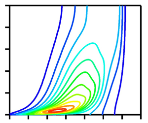
Next, we examine the homogeneous part of the energy density,  ${\tilde {Q}_{ii}}(y,s)/2$, appearing in (4.5). Figure 4(a) shows the contours of the pre-multiplied quantity $s{\tilde {Q}_{ii}}(y,s)/2$ in the $s$–
$s$– $y$ plane. The peak is located at $s = 3.2 \times {10^{ - 4}}$ and $y = 0.036$ ( ${y^ + } = 36$). The peak location with respect to $s$ increased as $y$ increased. The contour plots of $s{\tilde {Q}_{ii}}(y,s)/2$ are very similar to those of ${r_y}E(y,{r_y})$ shown by Hamba (Reference Hamba2018). The difference is that the latter shows a negative value in the region very close to the wall, whereas the former is non-negative because of its definition. Figure 4(b) shows the profiles of $s{\tilde {Q}_{ii}}(y,s)/2$ as functions of $s$ at four $y$ locations. The shift of the peak towards large scales is clearly shown. The profile for $y = 0.79$ in the core region is similar to that of the homogeneous isotropic turbulence shown in figure 2(b) because the local Reynolds number is rather large. The profiles quickly decay at $s > 1$, unlike in the case of homogeneous isotropic turbulence, because the integral region is limited to $0 \leqslant y \leqslant 2$ in the channel flow.

Figure 4. Profiles of pre-multiplied homogeneous part  $s\tilde {Q}_{ii}(y,s)/2$ in the case of one-dimensional filtering: (a) contour plots in the $s$–
$s$– $y$ plane and (b) profiles as functions of $s$ at four $y$ locations.
Although the homogeneous part is non-negative, the energy density  ${\hat {Q}_{ii}}(y,s)/2$ can be negative because of the inhomogeneous part. We examined the homogeneous and inhomogeneous parts of the energy density at a fixed $y$ location. Figure 5 shows the profiles of the pre-multiplied energy density and its two parts given by (4.5) as functions of $s$ at two $y$ locations. In figure 5(a) for ${y^ + } = 29$, the homogeneous part is positive in the entire $s$ region, whereas the inhomogeneous part shows both positive and negative values. Because the inhomogeneous part is not very large, the total value is always positive. In contrast, in figure 5(b) for ${y^ + } = 2.9$, the inhomogeneous part has a large negative value at $s \sim 10^{-4}$, and the resulting total value also shows a negative value. Therefore, the energy density ${\hat {Q}_{ii}}(y,s)/2$ can be negative in the region very close to the wall because of the inhomogeneous effect.

Figure 5. Profiles of pre-multiplied energy density  $s\hat {Q}_{ii}(y,s)/2$ and its two parts given by (4.5) in the case of one-dimensional filtering as functions of $s$ (a) for $y^{+} = 29$ and (b) for $y^{+} =2.9$.
As shown in figure 5, the inhomogeneous part changes its sign as  $s$ increases. Its sign is closely related to the profile of the energy ${\bar {Q}_{ii}}(y,s)/2$, as shown by (4.5). Figure 6 shows the profiles of ${\bar {Q}_{ii}}(y,s)/2$ as functions of $y$ for four scales. The vertical line denotes the location at ${y^ + } = 29$, where the energy density is plotted in figure 5(a). The energy ${\bar {Q}_{ii}}(y,s)/2$ for $s = 0$ corresponds to the turbulent energy $K$. The energy for $s = {10^{ - 4}}$ shows a convex profile at ${y^ + } = 29$, which leads to a positive value for the inhomogeneous part at $s = {10^{ - 4}}$ in figure 5(a). However, the energy for $s = {10^{ - 3}}$ shows a slightly concave profile, which leads to a negative value for the inhomogeneous part at $s = {10^{ - 3}}$. Despite the very small variations, the energy for $s = {10^{ - 2}}$ has a convex profile that leads to a positive value at $s = {10^{ - 2}}$.

Figure 6. Profiles of energy  $\bar {Q}_{ii}(y,s)/2$ in the case of one-dimensional filtering for four scales as functions of $y$ (a) at $0 < y < 1$ and (b) at $0 < y^{+} < 100$. The vertical lines denote the location at $y = 0.029$ ( ${y^ + } = 29$).
The energy  ${\bar {Q}_{ii}}(y,s)/2$ is half the variance of the filtered velocity ${\bar {u}_i}({\boldsymbol {x}},s)$, which is affected by the original velocity ${u_i}({\boldsymbol {x'}})$ in the region where $\bar {G}(y - y',s)$ has a certain positive value. Here, we compare the profiles of $\bar {G}(y - y',s)$ and the velocity field, and discuss the reasons why the energy ${\bar {Q}_{ii}}(y,s)/2$ shows different profiles depending on $s$. Figure 7 shows the profiles of the turbulent energy $K$ and the filter function $\bar {G}(y - 0.029,s)$ for three scales as functions of ${y^ + }$. The vertical line denotes the location at ${y^ + } = 29$ ( $y = 0.029$). As shown in (D4) and (D5) in Appendix D, it is considered that at $y < 0$, the velocity components ${u_x}$ and ${u_z}$ have mirror-symmetric profiles with respect to the wall. To represent their intensity, we plot a mirror-symmetric profile of $K$ in figure 7. The profile of $K$ has two peaks at ${y^ + } = \pm 18$ and a deep valley at ${y^ + } = 0$. The reason for the dependence of the profile of ${\bar {Q}_{ii}}(y,s)/2$ on $s$ can be explained as follows. In the case of $s = {10^{ - 4}}$, only the peak at ${y^ + } = 18$ is located within the non-zero region of $\bar {G}(y - 0.029,s)$, which leads to a convex profile of ${\bar {Q}_{ii}}(y,s)/2$ for $s = {10^{ - 4}}$, as shown in figure 6. In the case of $s = {10^{ - 3}}$, both the peak at ${y^ + } = 18$ and the deep valley at ${y^ + } = 0$ are located in the region. The strong effect of the valley gives rise to a concave profile of ${\bar {Q}_{ii}}(y,s)/2$ for $s = {10^{ - 3}}$. In the case of $s = {10^{ - 2}}$, the profile of $\bar {G}(y - 0.029,s)$ is so wide that the total of two peaks and one valley can effectively act as one peak, which could lead to a convex profile of ${\bar {Q}_{ii}}(y,s)/2$ for $s = {10^{ - 2}}$. Therefore, ${\bar {Q}_{ii}}(y,s)/2$ at ${y^ + } = 29$ shows different profiles depending on $s$. A similar explanation is possible for ${\bar {Q}_{ii}}(y,s)/2$ at ${y^ + } = 2.9$. In this case, the effect of the valley at ${y^ + } = 0$ is so significant that the inhomogeneous part shows a large negative value at ${10^{ - 5}} < s < {10^{ - 4}}$, as shown in figure 5(b).

Figure 7. Profiles of turbulent energy  $K$ and filter functions $\bar {G}(y-0.029,s)$ for three scales as functions of $y^{+}$. The vertical line denotes the location at ${y^ + } = 29$.
The inhomogeneous part represents the explicit effect of inhomogeneity as discussed above. At the same time, the effect of inhomogeneity is also present in the homogenous part because of the inhomogeneous distribution of the velocity variance. In figure 3, the homogeneous part shows an inhomogeneous profile and its peak location is apart from the wall compared with the peak of the kinetic energy. The peak of  $s{\tilde {Q}_{ii}}(y,s)/2$ in figure 4 occurs at $(s^{+})^{1/2} \simeq 18$ for $y^{+}=36$. The length scale $(s^{+})^{1/2}$ is approximately half the distance to the wall and suggests the effect of the wall on the size of eddies.
So far, we have examined the homogeneous and inhomogeneous parts of the energy density in the case of one-dimensional filtering. To assess the properties of channel flow corresponding to the three-dimensional energy spectrum, three-dimensional filtering is adopted here. In the case of three-dimensional filtering, the filtered velocity  ${\bar {u}_i}({\boldsymbol {x}},s)$ is defined as
 \begin{equation} {\bar{u}_i}({\boldsymbol{x}},s) = \int_{0}^{4{\rm \pi} } {\mathrm{d} x'} \int_{ 0}^2 {\mathrm{d} y'} \int_{0}^{2{\rm \pi} } {\mathrm{d}z'}\,\bar{G}({\boldsymbol{x}},{\boldsymbol{x'}},s){u_i}({\boldsymbol{x'}}) . \end{equation}
The homogeneous and inhomogeneous parts of the energy density and turbulent energy are given by (4.5) and (4.6), respectively. These are the same equations as in the one-dimensional case because the averaged quantities are only dependent on  $y$, and their derivatives with respect to $x$ and $z$ disappear. Figure 8 shows the profiles of the turbulent energy and its three parts given by (4.6) as functions of $y$. The residual part ${\bar {Q}_{ii}}(y,\infty )/2$ is negligibly small because ${\bar {u}_i}({\boldsymbol {x}},\infty )$ is very small in the three-dimensional case. The magnitude of the inhomogeneous part is also small compared with the one-dimensional case, while the homogeneous part is nearly equal to the total value. The inhomogeneous effect of the turbulent energy at remote positions decreased in the three-dimensional case because the energy density at large scales decreased, as shown in figure 2(b). Nevertheless, the inhomogeneous part shows a large negative value in the region very close to the wall at ${y^ + } < 10$, as shown in figure 8(b).

Figure 8. Profiles of turbulent energy  $K$ and its three parts given by (4.6) in the case of three-dimensional filtering as functions of $y$ (a) at $0 < y < 1$ and (b) at $0 < y^{+} < 50$.
Next, we examine the homogeneous part of the energy density,  ${\tilde {Q}_{ii}}(y,s)/2$, which appears in (4.5). Figure 9(a) shows the contours of the pre-multiplied quantity $s{\tilde {Q}_{ii}}(y,s)/2$ in the $s$–
$s$– $y$ plane. The peak is located at $s = 1.1 \times {10^{ - 4}}$ and $y = 0.026$ ( ${y^ + } = 26$). The scale $s$ is smaller and the $y$ location is closer to the wall compared with the one-dimensional case shown in figure 4(a). The peak location with respect to $s$ increases as $y$ increases, as in the case shown in figure 4(a). Figure 9(b) shows the profiles of $s{\tilde {Q}_{ii}}(y,s)/2$ as functions of $s$ at four $y$ locations. The values of the homogeneous part are greater than those of the one-dimensional case shown in figure 4(b), whereas their peak locations shift towards smaller scales. This situation is the same as the energy density for homogeneous isotropic turbulence shown in figure 2(b).

Figure 9. Profiles of the pre-multiplied homogeneous part  $s\tilde {Q}_{ii}(y,s)/2$ in the case of three-dimensional filtering: (a) contour plots in the $s$–
$s$– $y$ plane and (b) profiles as functions of $s$ at four $y$ locations.
Figure 10 shows the profiles of the pre-multiplied energy density  $s\hat {Q}_{ii}(y,s)/2$ and its two parts given by (4.5) as functions of $s$ at two $y$ locations. The relative importance of the inhomogeneous part is small compared with the one-dimensional case shown in figure 5. In particular, the positive profiles of the inhomogeneous part at large scales shown in figure 5 disappear in figure 10. Nevertheless, in figure 10(b), a large negative value of the inhomogeneous part at small scales leads to a negative value of the total or the energy density ${\hat {Q}_{ii}}(y,s)/2$ at ${y^ + } = 2.9$, even in the three-dimensional case.

Figure 10. Profiles of pre-multiplied energy density  $s\hat {Q}_{ii}(y,s)/2$ and its two parts given by (4.5) in the case of three-dimensional filtering as functions of $s$ (a) for $y^{+} = 29$ and (b) for $y^{+} =2.9$.
Figure 11 shows the profiles of  ${\bar {Q}_{ii}}(y,s)/2$ as functions of $y$ for four scales. The vertical line denotes the location at ${y^ + } = 29$ ( $y = 0.029$). As in the case in figure 6, a convex profile for $s = {10^{ - 4}}$ and a concave profile for $s = {10^{ - 3}}$ at $y^{+}=29$ can account for the positive and negative values of the inhomogeneous part shown in figure 10(a), respectively. Similarly, a concave profile of ${\bar {Q}_{ii}}(y,s)/2$ for $s = {10^{ - 4}}$ at ${y^ + } = 2.9$ leads to a large negative value for the inhomogeneous part, as shown in figure 10(b), which can account for the negative value of the energy density ${\hat {Q}_{ii}}(y,s)/2$ at ${y^ + } = 2.9$.

Figure 11. Profiles of energy  $\bar {Q}_{ii}(y,s)/2$ in the case of three-dimensional filtering for four scales as functions of $y$ (a) at $0 < y < 1$ and (b) at $0 < y^{+} < 100$. The vertical lines denote the location at $y = 0.029$ ( ${y^ + } = 29$).
As shown in figure 8, the turbulent energy  $K$ disappears at $y=0$, whereas the homogeneous and inhomogeneous parts show positive and negative values, respectively. Although the no-slip condition causes the velocity to disappear at $y=0$, the filtered velocities do not disappear because the velocity at $y>0$ contributes to some extent; the homogeneous part of the turbulent energy can take a positive value at the wall. It is well known that the energy dissipation rate $\varepsilon$ takes a positive value at the wall although the turbulent energy $K$ itself disappears. In the budget equation of $K$, a negative value of the dissipation term is balanced by a positive value of the viscous diffusion term. This budget indicates that the energy that flowed in by viscous diffusion dissipated at the wall. We can consider that the energy that flows in creates the positive homogeneous part at the wall and then the latter dissipates owing to the viscosity. In fact, the value of the homogeneous part of the energy density for $s=0$ is closely related to the dissipation rate, as shown in (3.6b).
Here, we attempt to understand the physical meaning of the inhomogeneous part of the energy density by considering the diffusion equation. We consider the one-dimensional case again for simplicity. As shown in Appendix A, the variance  ${\bar {Q}_{ii}}(x,s)$ also satisfies the diffusion equation given by (A5). Solving the diffusion equation, we obtain an expression for ${\bar {Q}_{ii}}(x,s)$ in (A6). By differentiating (A6) with respect to $s$, we obtain
 \begin{align} \tfrac{1}{2}{\hat{Q}_{ii}}(x,s) &= \tfrac{1}{2}{\tilde{Q}_{ii}}(x,s) - \int_0^s {\mathrm{d}s'} \int_{ - \infty }^\infty {\mathrm{d} x'} \,\hat{G}(x - x',s - s')\tfrac{1}{2}{\tilde{Q}_{ii}}(x',s')\nonumber\\ &\quad + \int_{ - \infty }^\infty {\mathrm{d} x'} \,\hat{G}(x - x',s)K(x') . \end{align}
We can see that the inhomogeneous part that appears in (2.28) is further divided into two parts: the second and third terms on the right-hand side of (4.8). If the turbulence is homogeneous and the averaged quantities are not dependent on  $x$, then the second and third terms disappear because $\int _{ - \infty }^\infty {\mathrm {d} x'} \,\hat {G}(x - x',s) = 0$. Equation (4.8) implies that the inhomogeneous part consists of the term representing the inhomogeneity of the homogeneous part ${\tilde {Q}_{ii}}(x',s')/2$ and the term representing that of the turbulent energy $K(x')$. In particular, the expression suggests that for the scale decomposition of the turbulent energy $K$ at position $x$, not only the homogeneous part ${\tilde {Q}_{ii}}(x,s)/2$ at the same position but also that at remote positions are necessary. This non-local contribution is similar to the expression for ${u_i}(x)$ in terms of ${\tilde {u}_i}(x,s)$ given by (2.22). Therefore, if the contribution from remote positions is allowed to reconstruct the turbulent energy $K$, the homogeneous part ${\tilde {Q}_{ii}}(x,s)/2$ can also be interpreted as the energy density itself. In fact, the volume integral of the turbulent energy is equal to the volume and scale integrals of ${\tilde {Q}_{ii}}(x,s)/2$, even for inhomogeneous turbulence, as follows:
 \begin{equation} \int_{V} {\mathrm{d} x} \,K(x) = \int_{V} {\mathrm{d} x} \int_0^\infty {\mathrm{d}s\tfrac{1}{2}} {\tilde{Q}_{ii}}(x,s) , \end{equation}
where boundary terms are omitted.
In addition to the second-order statistics examined in the present analysis, the third-order statistics are also important. The third-order moments including the energy flux in the scale space must be useful in examining the energy transport in channel flow. In fact, an inverse energy cascade in channel flow was observed in the analysis of the generalised Kolmogorov equation (Cimarelli et al. Reference Cimarelli, De Angelis and Casciola2013, Reference Cimarelli, De Angelis, Jiménez and Casciola2016) and in that of the previous energy densities (Hamba Reference Hamba2015, Reference Hamba2018). The energy flux in the scale space based on the present formulation and its relation to the inhomogeneity should be investigated in future work.
5. Conclusions
A new expression for the energy density in the scale space is proposed using three filtered velocities. The new expression consists of homogeneous and inhomogeneous parts. The homogeneous part is expressed in terms of the variance of the filtered velocity and is always non-negative. The inhomogeneous part is proportional to the second derivative of the variance of the filtered velocity. The energy density is non-negative for homogeneous turbulence because only the homogeneous part remains non-zero. It is shown that the turbulence inhomogeneity can cause a negative value of the energy density. By integrating the energy density with respect to scale, we obtain an expression for the turbulent kinetic energy that is also decomposed into homogeneous and inhomogeneous parts.
DNS data of homogeneous isotropic turbulence were first used to evaluate the homogeneous part of the energy density. The profiles of the energy density as functions of scale were compared between cases of one- and three-dimensional filtering. The homogeneous part plays a similar role as the energy spectrum. DNS data of a turbulent channel flow were then used to evaluate the homogeneous and inhomogeneous parts of the energy density and turbulent energy. In the case of one-dimensional filtering, the inhomogeneous part of the turbulent energy showed fairly large values near the wall and at the channel centre. The contour plots of the homogeneous part of the energy density were similar to those of the previous energy density. The inhomogeneous part of the energy density changed its sign depending on the scale. Its positive and negative values were determined by the convex and concave profiles of the filtered-velocity variance near the wall, respectively. It was shown that a concave profile of the filtered-velocity variance at the wall accounts for the negative value of the energy density in the region very close to the wall. In the case of three-dimensional filtering, the value of the inhomogeneous part of the turbulent energy is relatively small. Nevertheless, the homogeneous and inhomogeneous parts of the energy density show profiles similar to those in the one-dimensional case.
We formulated the scale decomposition of the turbulent energy using filtered velocities in a systematic manner. The variations in the filtered velocity and its variance with increasing scale are related to the diffusion equations. One of the filtered velocities corresponds to a continuous wavelet transform of the velocity field. This formulation is expected to pave the way for a better understanding of inhomogeneous turbulence. For example, the energy transfer between different scales and the scale decomposition of two-point correlations should be examined in future work. It would also be interesting to formulate a statistical theory using filtered velocities to improve the turbulence models.
Funding
This work was supported by JSPS KAKENHI Grant number 20K04282.
Declaration of interests
The author reports no conflict of interest.
Appendix A. Diffusion equations for filtered velocity and its variance
We consider the following diffusion equation for  $\theta (x,t)$ at $- \infty < x < \infty$:
 \begin{equation} \frac{\partial }{{\partial t}}\theta (x,t) = \nu \frac{{{\partial ^2}}}{{\partial {x^2}}}\theta (x,t) + {\theta _S}(x,t) , \end{equation}
where  $\nu$ is the diffusivity and ${\theta _s}(x,t)$ is a source term. The solution of (A1) can be expressed in terms of the source term and initial value as follows:
 \begin{align} \theta (x,t) &= \int_0^t {\mathrm{d}t'} \int_{ - \infty }^\infty {\mathrm{d} x'} \frac{1}{{{{[4{\rm \pi} \nu (t - t')]}^{1/2}}}}\exp \left[ { - \frac{{{{(x - x')}^2}}}{{4\nu (t - t')}}} \right]{\theta _S}(x',t')\nonumber\\ &\quad + \int_{ - \infty }^\infty {\mathrm{d}\kern0.05em x'} \frac{1}{{{{(4{\rm \pi} \nu t)}^{1/2}}}}\exp \left[ { - \frac{{{{(x - x')}^2}}}{{4\nu t}}} \right]\theta (x',0) . \end{align}
 As shown in (2.18b), the filtered velocity  $\bar {u}_{i}(x,s)$ satisfies
 \begin{equation} \frac{\partial }{{\partial s}}\bar{u}_{i}(x,s) = \frac{1}{2}\frac{{{\partial ^2}}}{{\partial {x^2}}}{\bar{u}_i}(x,s) . \end{equation}
If we consider the scale  $s$ as the time, (A3) can be the diffusion equation where the viscosity $\nu$ is $1/2$ and no source term is involved. The solution of (A3) can then be written as
 \begin{align} {\bar{u}_i}(x,s) = \int_{ - \infty }^\infty {\mathrm{d}\kern0.05em x'} \frac{1}{{{{(2{\rm \pi} s)}^{1/2}}}}\exp \left[ { - \frac{{{{(x - x')}^2}}}{{2s}}} \right]{\bar{u}_i}(x',0) = \int_{ - \infty }^\infty {\mathrm{d} x'} \,\bar{G}(x - x',s){u_i}(x') , \end{align}
which agrees with (2.16). In general, the profile of the filtered velocity becomes smoother as the scale increases. Such a variation of the profile with increasing scale is expressed in terms of the time evolution of the diffusion equation solution.
Equation (2.28) shows that the variance  ${\bar {Q}_{ii}}(x,s)$ also satisfies the diffusion equation
 \begin{equation} \frac{\partial }{{\partial s}}{\bar{Q}_{ii}}(x,s) = \frac{1}{2}\frac{{{\partial ^2}}}{{\partial {x^2}}}{\bar{Q}_{ii}}(x,s) - {\tilde{Q}_{ii}}(x,s) , \end{equation}
where the source term is given by the homogeneous part of the energy density. The solution of (A5) can be written as
 \begin{align} {\bar{Q}_{ii}}(x,s) &={-} \int_0^s {\mathrm{d}s'} \int_{ - \infty }^\infty {\mathrm{d} x'} \frac{1}{{{{[2{\rm \pi} (s - s')]}^{1/2}}}}\exp \left[ { - \frac{{{{(x - x')}^2}}}{{2(s - s')}}} \right]{\tilde{Q}_{ii}}(x',s')\nonumber\\ &\quad + \int_{ - \infty }^\infty {\mathrm{d}\kern0.05em x'} \frac{1}{{{{(2{\rm \pi} s)}^{1/2}}}}\exp \left[ { - \frac{{{{(x - x')}^2}}}{{2s}}} \right]{\bar{Q}_{ii}}(x',0)\nonumber\\ &={-} \int_0^s {\mathrm{d}s'} \int_{ - \infty }^\infty {\mathrm{d} x'} \,\bar{G}(x - x',s - s'){\tilde{Q}_{ii}}(x',s') + \int_{ - \infty }^\infty {\mathrm{d} x'} \,\bar{G}(x - x',s){Q_{ii}}(x') . \end{align}
By differentiating (A6) with respect to  $s$, we obtain (4.8).
Appendix B. Filtered velocity and continuous wavelet transform
The continuous wavelet transform of  $f(x)$ and its inverse transform are written as (Daubechies Reference Daubechies1992)
 \begin{gather} ({W_\psi }f)(b,a) = \frac{1}{{\sqrt a }}\int_{ - \infty }^\infty {f(x)} \overline{\psi \left( {\frac{{x - b}}{a}} \right)}\mathrm{d} x , \end{gather}
 \begin{gather}f(x) = \frac{2}{{{C_\psi }}}\int_0^\infty {\left[ {\int_{ - \infty }^\infty {({W_\psi }f)(b,a)\frac{1}{{\sqrt a }}} \psi \left( {\frac{{x - b}}{a}} \right)\mathrm{d}b} \right]\frac{{\mathrm{d}a}}{{{a^2}}}} , \end{gather}
respectively, where  $\bar {\cdot }$ denotes the complex conjugate and
 \begin{equation} {C_\psi } = \int_{ - \infty }^\infty {\mathrm{d}k} {\left| {\hat{\psi} (k)} \right|^2}/\left| k \right| ,\quad \hat{\psi} (k) = \int_{ - \infty }^\infty {\mathrm{d} x} \,\psi (x)\exp ( - \mathrm{i}kx) . \end{equation}
The filtered velocity  ${\tilde {u}_i}(x,s)$ defined as (2.20) can be considered a continuous wavelet transform of ${u_i}(x)$ as follows:
 \begin{equation} {\tilde{u}_i}(x,s) = \frac{1}{{{{(2s)}^{3/4}}}}({W_\psi }{u_i})(x,{(2s)^{1/2}}) , \end{equation}
with
 \begin{equation} \psi (x) = \frac{2}{\sqrt{ {\rm \pi}}}x\exp ( - {x^2}) . \end{equation}
In contrast to the wavelet analysis of turbulence, where even Mexican-hat-type functions are frequently used for  $\psi (x)$ (Farge Reference Farge1992; Schneider & Vasilyev Reference Schneider and Vasilyev2010), an odd function was used in (B5). A similar wavelet function was used by Altaisky et al. (Reference Altaisky, Hnatich and Kaputkina2018) to analyse the stirring force of the statistical theory of turbulence.
Appendix C. Formulation in the case of three-dimensional filtering
In the case of three-dimensional filtering, the first filtered velocity is defined as
 \begin{equation} {\bar{u}_i}({\boldsymbol{x}},s) = \bar{F}(s)*{u_i}({\boldsymbol{x}}) = \int {\mathrm{d}{\boldsymbol{x'}}} \,\bar{G}({\boldsymbol{x}} - {\boldsymbol{x'}},s){u_i}({\boldsymbol{x'}}) , \end{equation}
where
 \begin{align} \bar{G}({\boldsymbol{x}} - {\boldsymbol{x'}},s) = \frac{1}{{{{(2{\rm \pi} s)}^{3/2}}}}\exp \left[ { - \frac{{{{({\boldsymbol{x}} - {\boldsymbol{x'}})}^2}}}{{2s}}} \right] ,\quad \int {\mathrm{d}{\boldsymbol{x}}} = \int_{ - \infty }^\infty {\mathrm{d}\kern0.05em x} \int_{ - \infty }^\infty {\mathrm{d} y} \int_{ - \infty }^\infty {\mathrm{d}z} . \end{align}
By differentiating (C2) with respect to  $s$, we can obtain the second filtered velocity
 \begin{equation} {\hat{u}_i}({\boldsymbol{x}},s) \equiv{-} \frac{\partial }{{\partial s}}{\bar{u}_i}({\boldsymbol{x}},s) = \hat F(s)*{u_i}({\boldsymbol{x}}) = \int {\mathrm{d}{\boldsymbol{x'}}} \,\hat{G}({\boldsymbol{x}} - {\boldsymbol{x'}},s){u_i}({\boldsymbol{x'}}) , \end{equation}
where
 \begin{align} \hat{G}({\boldsymbol{x}} - {\boldsymbol{x'}},s) \equiv{-} \frac{\partial }{{\partial s}}\bar{G}({\boldsymbol{x}} - {\boldsymbol{x'}},s) = \frac{1}{{{{(2{\rm \pi} s)}^{3/2}}}}\left[ {\frac{3}{{2s}} - \frac{{{{({\boldsymbol{x}} - {\boldsymbol{x'}})}^2}}}{{2{s^2}}}} \right]\exp \left[ { - \frac{{{{({\boldsymbol{x}} - {\boldsymbol{x'}})}^2}}}{{2s}}} \right] . \end{align}
The filter function and filtered velocity satisfy the three-dimensional diffusion equations as follows:
 \begin{equation} \frac{\partial }{{\partial s}}\bar{G}({\boldsymbol{x}} - {\boldsymbol{x'}},s) = \frac{1}{2}\frac{{{\partial ^2}}}{{\partial x_j^2}}\bar{G}({\boldsymbol{x}} - {\boldsymbol{x'}},s) ,\quad \frac{\partial }{{\partial s}}{\bar{u}_i}({\boldsymbol{x}},s) = \frac{1}{2}\frac{{{\partial ^2}}}{{\partial x_j^2}}{\bar{u}_i}({\boldsymbol{x}},s) . \end{equation}
The third filtered velocity can be defined as
 \begin{equation} \tilde{u}_i^{(j)}({\boldsymbol{x}},s) \equiv \frac{\partial }{{\partial {x_j}}}{\bar{u}_i}({\boldsymbol{x}},s) = {\tilde{F}^{(j)}}(s)*{u_i}({\boldsymbol{x}}) = \int {\mathrm{d}{\boldsymbol{x'}}} {\tilde{G}^{(j)}}({\boldsymbol{x}} - {\boldsymbol{x'}},s){u_i}({\boldsymbol{x'}}) , \end{equation}
where
 \begin{equation} {\tilde{G}^{(j)}}({\boldsymbol{x}} - {\boldsymbol{x'}},s) \equiv \frac{\partial }{{\partial {x_j}}}\bar{G}({\boldsymbol{x}} - {\boldsymbol{x'}},s) ={-} \frac{1}{{{{(2{\rm \pi} s)}^{3/2}}}}\frac{{{x_j} - {x'_j}}}{s}\exp \left[ { - \frac{{{{ ( {\boldsymbol{x}} - {\boldsymbol{x'}})}^2}}}{{2s}}} \right] . \end{equation}
It should be noted that the third filtered velocity is effectively the velocity gradient with three components  $j = 1, 2, 3$. The original velocity can be given by obtaining the sum over $j$ as follows:
 \begin{equation} {u_i}({\boldsymbol{x}}) ={-} \int_0^\infty {\mathrm{d}s} {\tilde{F}^{(j)}}(s)*\tilde{u}_i^{(j)}({\boldsymbol{x}},s) ={-} \int_0^\infty {\mathrm{d}s} \int {\mathrm{d}{\boldsymbol{x'}}}\, {\tilde{G}^{(j)}}({\boldsymbol{x}} - {\boldsymbol{x'}},s)\tilde{u}_i^{(j)}({\boldsymbol{x'}},s) . \end{equation}
Finally, the homogeneous and inhomogeneous parts of the energy density are expressed in a similar manner as
 \begin{equation} \frac{1}{2}{\hat{Q}_{ii}}({\boldsymbol{x}},s) = \frac{1}{2}{\tilde{Q}_{ii}}({\boldsymbol{x}},s) - \frac{1}{4}\frac{{{\partial ^2}}}{{\partial x_k^2}}{\bar{Q}_{ii}}({\boldsymbol{x}},s) . \end{equation}
Appendix D. Treatment of filter function at the wall
We consider the  $0 < y < \infty$ region, where the wall is located at $y = 0$. We then define the one-dimensional filtered velocity as
 \begin{equation} {\bar{u}_i}(x,y,z,s) = \int_0^\infty {\mathrm{d} y'} \,\bar{G}(y,y',s){u_i}(x,y',z) . \end{equation}
The filter function given by (2.13) can be used apart from the wall, where  $y$ is much greater than ${s^{1/2}}$, whereas some modifications are required near the wall. Here, we assume that the filter function is a solution of (4.2a,b) with some boundary conditions at $y = 0$. The first candidate of the boundary condition is
 \begin{equation} \frac{\partial }{{\partial y}}\bar{G}(y,y',s) = 0 , \end{equation}
which is a type of free-slip condition. This is adequate because the following condition is satisfied:
 \begin{equation} \int_0^\infty {\mathrm{d} y'} \,\bar{G}(y,y',s) = 1 . \end{equation}
The use of the free-slip condition is equivalent to the situation in which a mirror-symmetric velocity profile exists at  $y < 0$ as
 \begin{equation} {u_i}(x,y,z) = {u_i}(x,-y,z),\quad (y < 0) . \end{equation}
Therefore, the filter function obtained from (4.2a,b) with (D2) is equivalent to the summation of the two original filter functions as follows:
 \begin{align} {\bar{u}_i}(x,y,z,s) &= \int_0^\infty {\mathrm{d} y'} \,\bar{G}(y - y',s){u_i}(x,y',z) + \int_{ - \infty }^0 {\mathrm{d} y'} \,\bar{G}(y - y',s){u_i}(x, - y',z)\nonumber\\ & = \int_0^\infty {\mathrm{d} y'} (\bar{G}(y - y',s) + \bar{G}(y + y',s)){u_i}(x,y',z) . \end{align}
In this study, we adopt this type of filter function for  ${\bar {u}_x}$ and ${\bar {u}_z}$, but not for ${\bar {u}_y}$. This is because the $x$ and $z$ derivatives are commutative with the filtering but the $y$ derivative is not, as follows:
 \begin{gather} \frac{\partial }{{\partial x}}{\bar{u}_i}(x,y,z,s) = \int_0^\infty {\mathrm{d} y'} (\bar{G}(y - y',s) + \bar{G}(y + y',s))\frac{\partial }{{\partial x}}{u_i}(x,y',z), \end{gather}
 \begin{gather}\frac{\partial }{{\partial y}}{\bar{u}_i}(x,y,z,s) = \int_0^\infty {\mathrm{d} y'} (\bar{G}(y - y',s) - \bar{G}(y + y',s))\frac{\partial }{{\partial y'}}{u_i}(x,y',z) , \end{gather}
and the solenoidal condition  $\partial {\bar {u}_i}/\partial {x_i} = 0$ cannot be satisfied.
We then consider the second boundary condition
 \begin{equation} \bar{G}(y,y',s) = 0 , \end{equation}
which is a type of no-slip condition. This is equivalent to the situation in which an anti-mirror-symmetric velocity profile exists at  $y < 0$ as
 \begin{equation} {u_i}(x,y,z) ={-} {u_i}(x, - y,z),\quad (y < 0), \end{equation}
and the filtered velocity is written as
 \begin{align} {\bar{u}_i}(x,y,z,s) &= \int_0^\infty {\mathrm{d} y'} \,\bar{G}(y - y',s){u_i}(x,y',z) - \int_{ - \infty }^0 {\mathrm{d} y'}\, \bar{G}(y - y',s){u_i}(x, - y',z)\nonumber\\ &= \int_0^\infty {\mathrm{d} y'} (\bar{G}(y - y',s) - \bar{G}(y + y',s)){u_i}(x,y',z) . \end{align}
The  $y$ derivative of (D10) can then be written as
 \begin{equation} \frac{\partial }{{\partial y}}{\bar{u}_i}(x,y,z,s) = \int_0^\infty {\mathrm{d} y'} (\bar{G}(y - y',s) + \bar{G}(y + y',s))\frac{\partial }{{\partial y'}}{u_i}(x,y',z) , \end{equation}
where the filter functions are the same as those in (D6). Therefore, we adopt the filter function with the boundary condition in (D8) for  ${\bar {u}_y}$ to satisfy the solenoidal condition $\partial {\bar {u}_i}/\partial {x_i} = 0$.


 Open access