


1. Introduction
Avalanche forecasting, in our context, means the daily assessment of the avalanche hazard for a given region, i.e. forecasting at the meso-scale (Reference McClung and SchaererMcClung and Schaerer, 1993). The resulting avalanche warnings and recommendations for the public should describe the avalanche situation, i.e. give information about the place, the time and the probability of release for a specific type of avalanche (slab or sluff, large or small, wet or dry). The most convenient way to handle this sort of information is to summarize it as a degree of avalanche hazard. Since 1985, in Switzerland, the degree of hazard has been defined in descending order by the release probability, the areal extent of the instabilities and the size of the avalanches (Reference FöhnFöhn. 1985). The scale is generally based on the snow-cover stability. It copies the development or stepping of the most typical avalanche situations and hence is not linear. The intensity of an avalanche situation increases strongly from one degree to another, may be even exponentially. Consequently, the frequency of the degrees of hazard decreases accordingly with increasing degree of hazard (Fig. 1). Any expert system should profit from this concept that was adopted in 1993 by the working group of the European avalanche-warning services. In this study, seven degrees of avalanche hazard are used according to the structure defined in 1985; details of the Swiss hazard scale have also been given by Reference McClung and SchaererMcClung and Schaerer (1993).

Fig. 1. Relative frequency of the verified degree of hazard in the Davos region: ten winter seasons including 1512 d are considered. Light columns (left) for the old Swiss seven-degree scale, dark columns (right) and values for the new European five-degree scale.
Since dry-slab avalanches represent the most important threat for skiers and back-country travellers, we focused on the hazard of dry-slab avalanches. During spring time, wet-snow avalanches are partly considered: the daily increase of the hazard due to warming during the day is not taken into account.
Reference LaChapelleLaChapelle (1980) described the technique for assessing the avalanche hazard: weather, snow and snow-cover data observed daily and measured at several locations representative for a given area are evaluated by human experts using their knowledge and long-term experience combined with individual intuition. Since then the procedure has not changed much. The core is still formed by the classical process of synopsis supplemented nowadays by different sorts of supporting tools (Fig. 2).
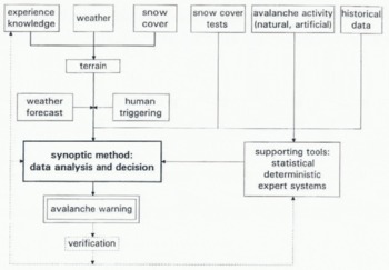
Fig. 2. The classical conventional method supplemented with different supporting tools to forecast the avalanche hazard on the regional scale.
However, the demands are steadily increasing: more frequent and more detailed information is desired. Tourism is still developing and, as in many other mountainous regions, the Alps have become one of the favourite playgrounds in Europe. Ski touring is wider ranging and more popular than it was previously. Nevertheless, the number of avalanche victims has not accordingly increased (Fig. 3),. which may be due to the better education and awareness of the skiers, presumably also due to the stabilizing effect of more frequent skiing after each snowfall period on popular slopes and hopefully due to better warning.

Fig. 3. Avalanche fatalities in the Swiss Alps 1964–65 to 1994–95. The fatalities are appointed to three categories describing where the avalanche accidents happened: in buildings, on communication lines (including controlled ski runs) and in the free terrain (back country). The 30 year average is about 28 fatalities, indicated by the thin broken line. The solid bold line shows a 5 year moving average. Percentage numbers give the proportion of fatalities in the free terrain (10 rear average) showing clearly the increasing number of fatalities in the free terrain, whereas the total number trend is stationary.
In the forecast processes nowadays, a lot of electronic tools are involved: acquisition, transfer and representation of the data, data base, snow-cover simulation,numerical weather forecast, decision-making tools and expert systems, and information distribution. Even so, the data that are measured are not the most relevant ones. What is really needed is the strength (Compressive, tensile and shear) of individual snow layers, the so-called low-entropy data (Reference LaChapelleLaChapelle, 1980) or class I data (Reference McClung and SchaererMcClung and Schaerer, 1993). The available data are just more or less appropriate to parameterize the relevant processes. The interpretation of these data is the most delicate task and hence many supporting tools have been developed for human experts. Because the avalanche hazard cannot (yet?) be calculated fully in a strict sense (by algorithms), this is a held for human experts and correspondingly for expert systems.
2. Present Approaches
The approach described by Reference LaChapelleLaChapelle (1980), the classical method, still forms the basis of the decision-making procedure of most avalanche-forecast services. Up till now, none of the supporting tools have been reliable enough to substitute for the human expert and will probably never be. But may they become an objective partner for “discussion”? A general overview of different methods has been given by Reference Föhn, Good, Bois and ObledFöhn and others (1977), Reference Buser, Föhn, Good, Gubler and SalmBuser and others (1985) and more recently by Reference McClung and SchaererMcClung and Schaerer (1993). In the following we focus on forecating models and tools.
Statistical approaches
The most popular statistical methods are the discriminant analysis and the nearest neighbours (Reference McClung and SchaererMcClung and Schaerer, 1993).
Already, in the 1970s the first studies using discriminant analysis had been performed to find the relevant parameters for avalanche forecasting (e.g. Reference PerlaPerla, 1970; Reference Judson and EricksonJudson and Erickson, 1973; Reference Armstrong, LaChapelle, Bovis. and IvesArmstrong and others, 1974; Reference Bois, Obled and GoodBois and others, 1975; Reference SalwaySalway, 1976). Snow and weather data are usually used together with observations of avalanche activity. New snow depth, temperature and wind speed, to mention some, have proved to be important. The results have confirmed the experience of the avalanche experts. But, as none of the parameters used is directly related to the process of avalanche formation, it has not been possible to evaluate the avalanche hazard.
The data used, the usual observed and measured parameters, are all index values. (The data used are those that are available and not those that are most relevant to the process of avalanche formation.) They are instructive to an expert and may give the correct hints to the key processes, such as settlement. However, the results of these statistical studies have improved the understanding and have helped to structure knowledge and finally to develop rule-based systems. Additionally, as the statistical models need long-term data, many valuable observations have been initialed. The accumulated data base may now be used to improve the memory of the expert.
Operational systems based on the statistical approach, and using a long-term data base, have been developed in several countries and are now widely used (Reference Buser, Bütler and GoodBuser and others, 1987; Reference Navarre, Guyomarc'h and GiraudNavarre and others, 1987; Reference McClung and TweedyMcClung, 1994;
Reference McClung and TweedyMcClung and Tweedy, 1994; Reference Mérindol and BrugnotMérindol, 1995) both for local and for regional avalanche forecasting. Except for the system developed by Reference McClung and TweedyMcClung and Tweedy (1994), which is a combination of the two statistical methods, all of them use the nearest-neighbour method. It is generally assumed that similar snow and weather conditions should lead to similar avalanche situations, i.e. that observed avalanches of similar past days should be representative of the present-day situation. A geometrical distance in the input parameter space is used in searching for similar situations. The Euclitdian distance between the actual-day data and the surrounding past-day data is in some models calculated directly in the input parameter space (Reference Buser, Bütler and GoodBuser and others. 1987); in other models, the input data are first transformed in the space of the principal components that was determined by the statistical analysis of the data base (Reference Mérindol and BrugnotMérindol. 1995) and then the Mahalanobis distance is used Reference McClung and TweedyMcclung and Tweedy, 1994). In some models, the input parameters are weighted according of the general experience of the expert forecaster (Reference Buser, Bütler and GoodBuser and others, 1987) and the weights may even vary according to the general weather type (Reference BolognesiBolognesi, 1993b). The output is generally based on the observed avalanches of the ten or 30 nearest neighbouring days. This information has to be evaluated by the forecaster. The simplest way to summarize this sort of information is to just separate between avalanche days and non-avalanche days (Reference Obled and GoodObled and Good, 1980). In addition to the list of the 30 nearest neighbours, Reference McClung and TweedyMcClung and Tweedy (1994) predicted the probability of avalanching by using discriminant analysis. For the forecasting of avalanches at Kootenay Pass (B.C., Canada) this probability is combined, using Baysian statistics, with the expert's opinion, made a priori, to take into account additional low-entropy data (e.g. the snow-cover situation) (Reference Weir and McClungWeir and McClung, 1994). In other models, a number is given as output according to the classification of observed avalanches used in the country (Reference Guyomarc'h and MérindolGuyomarc'h and Mérindol, 1994) or an avalanche index is calculated (Reference Navarre, Guyomarc'h and GiraudNavarre and others, 1987). These types of output are difficult to relate to the actual hazard in a given region. Hence, it is difficult to assess the real quality of these forecast models. They certainly improve the reflections of unexperienced forecasters and may influence experienced forecasters but rarely may they be called a decisive help in determining the degree of hazard in a given region.
Deterministic approaches
The aim of the deterministic approach is to simulate the avalanche release. Whereas the most relevant snow-cover processes may be modelled (Reference Brun, Martin, Simon, Cendre and ColeouBrun and others, 1989, Reference Brun, David, Sudul and Brunot1992) and some attempts have also been made to model the avalanche formation (Reference Gubler and BaderGubler and Bader, 1989), it is still almost impossible to simulate the range of the numerous avalanche-formation processes on a mountain slope—not to speak of a whole area. A possible way out is to use different methods, for example, to develop an expert system which analyzes the simulated snow-cover stratigraphy (Reference GiraudGiraud, 1991). Reference Föhn and HacchlerFöhn and Haechler (1978) developed a deterministic–statistical model which relates the snow accumulation by snowfall, wind and settlement to the avalanche activity. The model is appropriate to describe avalanche situations in periods of heavy snowfall.
Expert Systems
Expert systems Footnote * represent the idea of simulating the decision-making process of an expert. Most of them are symbolic computing systems, i.e. using rules which were formulated explicitly by human experts, e.g. MEPRA (Reference GiraudGiraud, 1991) and AVALOG (Reference BolognesiBolognesi, 1993a). The French system MEPRA analyzes the snow-cover stratigraphy; the snow profiles are simulated by the snow-cover model CROCUS (Reference Brun, Martin, Simon, Cendre and ColeouBrun and others, 1989) in parallel with meteorological data provided by SAFRAN (Reference Durand, Burn, Mérindol, Guyomarc'h, Lesaffre and MartinDurand and others, 1993), a model for optimal interpolation of meteorological data. AVALOG, assessing the avalanche hazard slope-by-slope, is an assisting tool for the efficient artificial release by explosives in the restricted area of a ski resort. Recently, a hybrid expert system has been developed using a neural network and rules extracted from the data base with neural network techniques (Reference Schweizer, Föhn, Schweizer, Ultsch, Schertler, Schmid, Tjoa and WerthnerSchweizer and others, 1994a, Reference Schweizer, Föhn, Schweizer and Hamzab). Reference BolognesiBolognesi (1993b) has developed another hybrid system called NX-LOG by combining the statistical model NXD (Reference Buser, Bütler and GoodBuser and others, 1987) and the rule-based system AVALOG. A further recent development is a rule-based expert system to interpret data from snow profiles with respect to snow stability (Reference McClungMcClung, 1995).
3. A New Approach with the Cybertek-Cogensys Judgment Processor
In 1989, we began a new approach with the idea of building a system for regional avalanche forcasting similar to the statistical ones but with a different method of searching for similar situations and with optimized input and output parameters, called DAVOS. We tried to include some of the relevant physical processes, i.e. elaborated input parameters and to give as a result directly what the avalanche forecaster would like to have: the degree of hazard (Reference Schweizer, Föhn and PlüssSchweizer and others, unpublished).
In 1991, we worked out a completely new approach, more process-oriented and partly rule-based, which tried to model the reasoning of the avalanche forecaster, called MODUL.
Both models are based on software for inductive decision-making: CYBERTEK-COGENSYSTM judgment processor (version 19), which is primarily used in the finance and insurance world.
The method: the judgment processor
The CYBERTEK-COGENSYSTM judgment processor is a commercially available software for inductive automatic decision-making. Since we had no access to the source code, we did not exactly know what the system does (however, it works). So, the algorithm cannot be given in all detail, but we shall try to outline the general idea below. So far, the core of the system may be considered a “black box”. The judgment processor is based on the fact that pragmatic experts deride, using their experience and intuition rather than explicit rules. The more complex a problem, the less structured is the knowledge. Experts are usually able to decide correctly and fast in a real situation. However, they are usually hardly able to explain their decisions completely following exact rules. The expert's approach is to choose the relevant data (which may differ substantially from one situation to another), to classify and to analyze the data and finally to reach a conclusion.
Building up a model involves the following steps:
-
1. A so-called judgment problem consists of a list of questions and the logic required to arrive at a judgment—that is, to reach a conclusion or make a decision — based on the answers to those questions. By specifying the questions–to be answered by yes/no, multiple choice or numerical responses—the mentor, the expert building up the system, defines the data needed to reach a specific decision and the criteria that are used to categorize or evaluate the data. That means for numerical questions that the possible answers must be grouped into so-called logical ranges (up to five ranges), so that the system can learn how the response is normally categorized. Numerical questions can take the form of calculations including conditions.
-
2. Once a problem has been defined, the mentor “teaches” the judgment processor by entering examples (real or realistic data) and interpreting the situations represented by those examples. By observing the relationship between the data and the mentor's decisions, the judgment processor builds a logical model that allows it to emulate the mentor's decisions. The more complex the problem the more situations are needed. However, as usual in case-based reasoning systems, the performance of the system increases fast at the beginning with increasing number of situations, reaches a plateau and finally may even decrease (Fig. 4).
-
3. The judgment processor calculates the so-called logical importance of each question based on the observation of the mentor's decision. The logical importance is a measure of how a particular question contributes to the logical model as a whole, based on how many situations within the knowledge base would become indistinguishable if that question were to be removed. Based on the logical importance, given as a number from 1 … 100, the questions are classified as so-called major or minor questions. The logical importance is continuously Updated, so the system can learn incrementally.

Fig. 4. A typical example of the performance of a case-based reasoning system with increasing Knowledge base over lime: the DAVOS4 model.
After sufficient training of the model by the mentor, the model performs the following steps to reach a conclusion for a new situation entered:
-
I. If a new situation is encountered, the system tries to give a proposition for the possible decision on the basis of the past known situations and on what is learned about the decision logic; particularly, the classification into major and minor questions based on the previously calculated logical importance is used. A new situation is similar to a known past situation from the knowledge base, if a certain number of the answers (usually 80%) to the major questions are within the same logical range. That means that primarily only the major questions are considered for searching for similar situations. Two past situations that are both similar to a new situation may hence coincide in different questions, e.g. if a problem consists of five major questions, four answers have to be in the same range, and hence five different possibilities exist for a similar situation, in addition to the case when a previous situation is found that coincides in all answers to the major questions. So similar situations need not consequently be near, in a geometrical sense in the parameters space, to the new situation.
-
II. The proposed decision is derived from the similar situations found using the so-called assertion level of the different similar situations. All questions and their logical importance are considered to determine the assertion level. It is a number (on a scale of 1–100 that reflects how closely the current situation compares to existing situations in the knowledge base. The closer the assertion level is to 100, the more similar this example is to previously encountered situations. The less the answers agree, the smaller is the assertion level, i.e. for each answer that does not agree, a certain amount is subtracted from 100, depending on the number of questions and the logical importance of the question; in the case of perfect agreement, a so-called full match, the assertion level is hence equal to 100.
-
III. The quality of the proposed decision, based on the similar situations found, is described by the so-called confidence level, an indicator of how certain the system is that its interpretation is appropriate to the current situation: an exclamation mark (!) for very confident, a period (.) for reasonably confident or a question mark (?) for not confident. A low level of confidence suggests that there are few situations that the system considers to be logically similar, or that those situations that are similar have conflicting interpretations. Additionally, the similar situations that are used to derive the decision with the according assertion level are also given as an explanation. If the system is not able to find a decision on the basis of the present knowledge base it gives the result “not possible to make an interpretation”, in the following simply called “no interpretation”.
In Figure 5 the different steps to reach a conclusion (described above) are summarized in strongly simplified graphical form. In Table 1 an example of the system output is given.
Table 1. Example of screen output: MODUL model, sub-problem Release probability new snow, 11 January, 1995 (see text for explanation of terms and Figure 8). The sub-problem has six input parameters; the system proposed the output large for the release probability, but it is not sure at all, so it puts a question mark. As explanation, four similar situations are given


Fig. 5. CYBERTEK-CONGENSYSTM Judgement Processor: the different steps to reach a conclusion are given (strongly simplified) for a problem with only three input parameters (X1, X2, X3) and one output parameter (“x” or “ + ”). (a) Input parameter space. (b) Categorization, leading to a cube (x1, x2, x3) of 125 identical boxes. (c) Reduction to the major parameters (x1, x3), i.e. projection to this plane. Selecting similar situations (all situations in the shaded squares) based on the following similarity condition: similar situations are all past situations with either x1 or x3 in the same category as the new situation. In the shaded squares are often several similar past situations; these situations that may have different output differ in the third (minor) parameter (x2). Based on the similar situations, referring to the logical importance and the minor parameter, the system proposes the result; in the above case, the proposed output would be “ + ”, with a confidence level of “?”, i.e. not confident, since there are too many similar situations with different output.

Fig. 5. CYBERTEK-CONGENSYSTM Judgement Processor: the different steps to reach a conclusion are given (strongly simplified) for a problem with only three input parameters (X1, X2, X3) and one output parameter (“x” or “ + ”). (a) Input parameter space. (b) Categorization, leading to a cube (x1, x2, x3) of 125 identical boxes. (c) Reduction to the major parameters (x1, x3), i.e. projection to this plane. Selecting similar situations (all situations in the shaded squares) based on the following similarity condition: similar situations are all past situations with either x1 or x3 in the same category as the new situation. In the shaded squares are often several similar past situations; these situations that may have different output differ in the third (minor) parameter (x2). Based on the similar situations, referring to the logical importance and the minor parameter, the system proposes the result; in the above case, the proposed output would be “ + ”, with a confidence level of “?”, i.e. not confident, since there are too many similar situations with different output.

Fig. 5. CYBERTEK-CONGENSYSTM Judgement Processor: the different steps to reach a conclusion are given (strongly simplified) for a problem with only three input parameters (X1, X2, X3) and one output parameter (“x” or “ + ”). (a) Input parameter space. (b) Categorization, leading to a cube (x1, x2, x3) of 125 identical boxes. (c) Reduction to the major parameters (x1, x3), i.e. projection to this plane. Selecting similar situations (all situations in the shaded squares) based on the following similarity condition: similar situations are all past situations with either x1 or x3 in the same category as the new situation. In the shaded squares are often several similar past situations; these situations that may have different output differ in the third (minor) parameter (x2). Based on the similar situations, referring to the logical importance and the minor parameter, the system proposes the result; in the above case, the proposed output would be “ + ”, with a confidence level of “?”, i.e. not confident, since there are too many similar situations with different output.
Since the search for similar situations forms the core of the method, it may be called, in the broadest sense, a nearest-neighbour method. However, the metric for searching for similar situations differs substantially from the commonly used distance measure, e.g. the Euclidian distance. The categorization of the input data, the classification into major and minor questions and the metric to search similar situations are all non-linear. Briefly summarized, the system weighs and classifies the categorized data, searches for similar situations strongly using the classification and categorization, derives a result from the similar situations, describes the quality of the result and finally lists the similar situations used for deriving the result together with the pertinent similarity measure. The advantage of the method is the strong concentration on the questions that are considered important. The fact that the majority of the answers to the major questions have to be in the same logical range makes the logical importance of a question, comparable to the weight used in a different system, to a decisive factor, in contrast to similar systems. So different versions of a model, as we will use, with the same questions but with different logical importance (calculated by the system, not given arbitrarily), leading to a different partition of major and minor questions, will find very different similar situations.
The application: the avalanche hazard
In our case the judgment problem is the avalanche hazard and the questions will be called input parameters and are, for example, the 3 d sum of new snow depth or the air temperature. The answers are the values of the input parameters in a real situation, e.g. 15 cm or −5°C. A real situation is hence described by the set of input parameter values (weather, snow and snow-cover data) for the given day. The logical ranges are, for example, in the case of the 3 d sum of new snow depth 0… 10, 10…30, 30…60. 60…120 and more than 120 cm. Finally, the decision or interpretation is the degree of hazard and in most versions of the model DAVOS see below) the altitude and the aspect of the most dangerous slopes.
4. Input, Output and Verification
We have chosen our input parameters (called questions in the judgment processor) from a data set which is believed to be representative of the region considered (Davos: about 50 km2): seven quantities are measured in the morning (at the experimental plot of SFISAR below Weissfluhjoch, 2540 m a.s.l., or at the little peak above the institute, the so-called Institutsgipfel, 2693 m a.s.l., by the automatic weather station of the Swiss Meteorological Institute), four quantities are prospective values for the day considered and ten quantities describe the actual state of the snow cover based on slope measurements performed about every 10 d. These principal data are given in Table 2.
Table 2. Principal data used in the two different DAVOS and MODUL models. D, Data used in the DAVOS model; M, Data used in the MODUL model

A description of the avalanche hazard is associated with each data set consisting of the above weather, snow and snow-cover data. It seems most appropriate to choose as output of an expert system exactly the structure that is usually used by forecasters. So the assisting tool “speaks” the same language as the forecaster. The question thus is: which degree of hazard describes the present avalanche situation and where is it located? Only the highest existing degree of hazard is given; the location is given by the slopes, described in terms of altitude and aspects, that are supposed to be the most dangerous in the region. So the given degree of hazard is not at all averaged over all aspects; it is definitely wrong to deal with averages in this context.
Therefore, the avalanche hazard is formulated first of all as degree of hazard (1…7). Secondly, the lower limit of the primarily endangered altitudes is given in steps of usually 200 m (> 1200, > 1600, > 1800, > 2000, > 2200, > 2400, >2500, >2600, >2800 ma.s.l.). Thirdly, the main aspect is described as either one of the mean directions (N, NE, E, SE, S, NW) and an according sector (±45°, ±67°, ±90°) or as extreme slopes or all slopes. The westerly sector is not so frequently endangered and if so, other aspects are also endangered, so it may be described by the other ones. If the hazard is given, for example, as 4. > 2400 ma.s.l., NE± 90°, this means high hazard on slopes with aspect from northwest to southeast above 2400 m a.s.l. Three examples are given in Figure 6.

Fig. 6. Three examples of how the regional avalanche hazard is described.
Verification
The “real” avalanche hazard that we use in the data base of the DAVOS model to teach the system is the result of an “a posteriori” critical assessment of the hazard, the so-called verification (Reference Föhn, Schweizer and Sivardière.Föhn and Schweizer, 1995). The verification has again the same structure as the model output. Otherwise, it is hardly possible to verify the avalanche hazard. Several studies on the verification of the avalanche hazard with the help of the so-called avalanche-activity index were not sufficiently successful (Reference Judson and KingJudson and King, 1985; Reference Giraud, Lafeuille and PahantGiraud and others, 1987; Reference RemundRemund, 1993). One reason is that in the case when no avalanches are present or observed, the avalanche hazard is not necessarily very low or even non-existent. Hence, it is obviously wrong to use the observed avalanche activity as the sole output parameter an assisting tool for regional avalanche forecasting.
The avalanche verification is not identical to the avalanche hazard described in the public avalanche warning. As the warning is prospective and the data base may be incomplete at the time of forecasting, the avalanche hazard might have been in fact larger or smaller. It is always easier to assess the avalanche hazard in hindsight! Operationally, the verification has been done some days later considering the observed avalanche activity (naturally and artificially released), the past weather conditions, the additional snow-cover tests, the back-country skiing activity and several other, partly personal observations. Snow-cover tests form an important part of the verification work. Like the real-time assessment itself, it is an expert task. We estimate that the verification describes the avalanche situation correctly in about 90% of the days and thus is much more accurate than the forecast. Using the degree of hazard from the avalanche forecast as output parameter would only be reasonable if the warning were always correct. An erroneous interpretation should not be enclosed in the data base. Comparing the forecasted degree of hazard to the verification, the forecast seems to be correct in about 70% of the days. So it seems obvious that the use of this type of verification represents a substantial improvement for the development of expert systems in the field of regional avalanche forecasting. Furthermore, verification is a prerequisite for evaluating the quality of any assisting tool for regional avalanche forecasting and, of course, also for improving the warning itself.
5. Models
Using the CYBERTEK-COGENSYSTM judgment processing system, we developed two different types of model: DAVOS and MODUL. The DAVOS model uses 13 weather, snow and snow-cover parameters and evaluates the degree of hazard, the altitude and the aspect. The model is exclusively data-based, whereas the MODUL model is both data- and rule-based. It uses 30 input parameters stepwise and the evaluation of the degree of hazard is the result of 11 interconnected judgment problems that are formulated according to the relevant processes. The system tries to model the decision-making process of an expert avalanche forecaster.
DAVOS model
General features: input, output and knowledge base
The DAVOS model uses the input parameters given in Table 3. Most of the values are calculated from nine principal values (Table 2) according to our experience. The idea was to take into account certain relevant processes, e.g. new snow settlement. Details have been given in Reference Schweizer, Föhn and PlüssSchweizer and others (unpublished). In the following some of the elaborated parameters are briefly described. The settlement-quotient parameter compares the increase in snow depth during the last 3 d with the sum of the new snow depth of the last 3 d. The smaller the value the better the Settlement. However, the settlement includes not only the new snow but also the old-snow settlement. The consolidation of the surface layer is described by the penetration-quotient parameter: the penetration depth today divided by the penetration depth yesterday. The heat transport into the snow cover is taken into account by a degree-day parameter: the sum of the positive air temperatures at noon of the last 2 d and the present day (prospectively) at 2000 ma.s.l. (the average altitude of the region considered). The snow transport is included by the blowing-snow parameter: the sum of additional wind-transported snow in leeward slopes over the last 3 d (Reference Föhn and HacchlerFöhn and Hacehler. 1978). The radiation index is an estimation (1, 2 or 3) of the daily total global solar radiation for the present day. 1 means below the long-term mean value for the given day, 2 about and 3 above, respectively. The snow-cover stability index (1 to 5) is an estimate of the state of the snow cover considering the snow profiles and Rutschblock tests that are available for the region. The depth of the critical layer is an estimation from the snow profiles and the Rutschblock tests. We usually dispose of the snow profile from the study plot and at least of one typical snow profile with a Rutschblock lest from a slope in the Davos area, the latter often performed by ourselves.
Table 3. Input parameters and logical ranges for the DAVOS model

Besides the input parameters, we have also chosen the ranges for each of the input parameters according to our experience. As mentioned above, each of the input data is associated with one of up to five logical ranges. After several years of data accumulation, we are finally able to check whether the chosen ranges were reasonable or not. Two examples based on the 9 year data base are given in Figure 7. Whereas the 3 d sum of the new snow depth seems to categorize quite well, compared to the verified degree of hazard, the settlement quotient shows no specific trend. This is in accord with the study of Reference PerlaPerla (1970) but it is in contrast to the opinion of experienced forecasters. That probably does not mean that the settlement quotient is not important at all; it might be relevant but only in certain situations, i.e. combinations of input data. Statistical methods, in particular univariate, do not tell the whole truth. The DAVOS model also does not consider the settlement quotient as important (Table 4).
Table 4. Values of the logical importance of the different versions of the DAVOS model. Bold figures indicate so-called major parameters


Fig. 7. Comparison of the 3 d sum of the new snow depth (above) and the settlement quotient (below) with the degree of hazard to check whether the logical ranges chosen categorize the data appropriately. Average degree of hazard for each category is also shown. The data base consists of 1361 situations from nine winters.
The output result is the avalanche hazard described as degree of hazard, altitude and aspect of the most dangerous slopes (see above).
The knowledge base of the DAVOS model consists of the daily data from nine winters (1 December–30 April), i.e. 1361 situations. During this time period, 22 situations were pairwise identical, i.e. each of the input parameters of the 2 d considered belong to the same logical range. About 700 000 000 situations are theoretically but, of course, not physically possible.
Different versions: DAVOS1, DAVOS2,DAV0S31/DAVOS32 and DAVOS4
The original version of the DAVOS model was called DAVOS1. The experience with this version has given rise to further versions. The values of the logical importance of the original DAVOS1 version (Table 4) show clearly that this version is hardly able to discriminate well. Twelve of the 13 input parameters are considered as major ones. As a consequence, looking for similar situations means that ten of the present-day input parameter values have to be in the same range as the past-day values. This represents a very strict condition for the similarity and results in a large number of uninterpretable situations. This fact seems definitely to be due to the desired output result that consists of three independent and equivalent components (degree of hazard, altitude and aspect).
In the case of different independent output results, the CYBFRTFK-COGENSYSTM judgment processor offers the possibility of choosing one of them as the dominant output result. Hence, we used a second version of the model DAVOS: DAYOS2. Whereas in the DAYOS1 version all three results are equally important, in the DAYOS2 version the first output result, the degree of hazard, is the dominant one. This leads to different values of the logical importance and accordingly to different interpretations. Most relevant is the small number (four) of major parameters and hence the better selection performance: hardly any uninterpretable situations. In the DAYOS2 version, the values of the logical importance seem to be closer to general experience than to the DAVOS1 version where, for example, the new snow depth has no importance at all. The reason is the sort of output result and the predominance of situations with no new snow.
From experience, it is obvious that it is quite important whether for a given day there is new snow or not. Hence, we tried to take into account this fact by developing two new versions: one for the more frequent situations without snowfall and the other for the situations with snowfall—the DAVOS31 and DAVOS32 versions, respectively. These two versions concentrate on the degree of hazard like the DAVOS2 version. The knowledge base of the DAVOS31 version consists of all days from the last nine winters, when the 3 d sum of new snow depth was less than 10 cm: the complementary set of days with the 3 d sum of new snow depth equal to or larger than 10 cm forms the knowledge base of the DAVOS32 version. The differences in the logical importance in the two versions are quite typical (Table 4). The values of the logical importance of the DAVOS31 (no new snow) version are similar to the logical importance of the original DAVOS1 version, whereas the logical importance of the DAVOS32 version (new snow) are similar to the ones of the DAYOS2 version. The numbers of major parameters are four and seven, respectively. for the DAVOS31 and DAVOS32 versions; so they should discriminate quite well.
Finally, the output result was reduced to the degree of hazard: DAVOS4. The DAVOS4 version is most appropriate for comparison with similar forecasting models and we hoped that due to the single type of output the DAVOS4 version should discriminate better than the other versions.
In all the different versions the input parameters describing the state of the snow cover proved to be important (Table 4).
MODUL Model
General features and structure
The experiences with the different versions of the DAVOS model, described above, directed us to try a different, more deterministic approach. Originally, we hoped that the DAVOS model, based on the judgment processor, would be able to choose the relevant parameters from the 13 input parameters according to the situation and generally somehow to recognize the hidden structure of reasoning behind it. Despite the satisfactory results of some of the versions of the DAVOS model (see section below), it seems that this aim was too ambitious; the problem seems to be too complex or the method not good enough. So we decided to “help” the system by structuring the input data. The design of the MODUL model is therefore quite similar to the way a pragmatic expert forecaster decides (Fig. 8).

Fig. 8. Structure of the MODUL model: 11 sub-problems and their relation. Shaded boxes are only considered in the case of new snow.
First of all, it is decisive whether there is new snow or not. Either the expert has to assess the new-snow stability or he/she directly assesses, without new snow, the old-snow stability which is often similar to the stability 1 d before, except if there is, for example, a large increase of heat transport and/or radiation. In he/she structures the input data according to the different steps in the decision process. If both the new-snow Stabilily and the old-snow stability, including both the effect of the weather as forecast for today, have been assessed, the two release probabilities are combined, Taking into account the effect of the terrain and of the skier as a trigger, the degree of hazard is finally determined. At the moment, only the degree of hazard is given; the altitude and the aspect of the most dangerous slopes, as given in most of the versions of the DAVOS model, have not yet been implemented.
Sub-problems
Each of the sub-problems as, for example, quality of new snow or stability of old snow represents a judgment problem, as described above, and is hence principally structured like the DAVOS model. The different sub-problems are just smaller than the DAVOS model, i.e. consist of only three to eight input parameters. Often, only three of the input parameters are considered as major parameters, This is a great advantage, since a much smaller knowledge base is sufficient to obtain good interpretations and the system usually learns faster and better from the logic behind the decision process. Sub-problems with only about five input parameters most of the time may find a similar past situation that is identical to the new situation, based on a knowledge base of only about 100 situations.
Implicit rules
It is even possible not only to build up the knowledge base with real situations but also to construct realistic situations by varying the major input parameters in a reasonable sense. This is impossible in the DAVOS model. So, if the expert feels sure about one of the sub-problems on the influence of one of the input parameters, maybe in combination with another one, he/she may systematically construct realistic situations and decide systematically. But this means nothing other than including a rule, not explicitly but implicitly. An example of such an implicit decision rule used in the sub-problem final merging is given in Table 5. This is, of course, rather exhausting work but the advantage is that one is more flexible in one's decision than in the case where one uses a strict explicit rule. It is easy for example to include non-linear relations. Furthermore, it is possible to construct extreme but still realistic situations that are usually rare but of course very important. So one of the disadvantages of principally statistic (or data)-based models using real data may he overcome. Finally, one arrives at a knowledge base that is a mixture of real, historic situations decided according to the verified hazard at those times and realistic situations directly decided according to general knowledge and experience. The problem is to have the appropriate mixture.
Table 5. General rule to decide on the degree of hazard in the sub-problem final merging; principally dependent on the combined (natural) release probability and the influence of the skier, but also dependent on the overall critical depth by the potential avalanche size and volume and on the depth of stable old snow by the terrain roughness

Input parameters
Thirty input parameters (Table 6) are used in 11 sub-problems interconnected partly by rules. Already, to obtain some of the data, a user with certain skills and experience is required. The output result of a sub-problem is usually used as an input parameter to another sub-problem that appears later on in the decision-making process. Many of the input-parameter values are calculated using rules that depend themselves on the input values. The overall critical depth for example depends, among other things, on the 3 d sum of blowing-snow depth that is only considered in certain situations when snowdrift is likely.
Table 6. Input parameters used in the MODUL model. The data are grouped according to the availability, i.e. how easy it is to get the data

Modifications
Due to the modular structure, it is easily possible to modify any of the sub-problems. Additionally, the relatively small number of input parameters in each sub-problem enables the knowledge base to adapt quickly to any modification, as for example adding a new input parameter. So the important sub-problem influence of the skier is steadily improved according to the results of specific study on slab-avalanche release triggered by a skier (Reference SchweizerSchweizer, 1993). In the sub-problem snow-profile analysis, the snow profile with Rutschblock test is roughly interpreted, an aim that would actually need an expert system itself. Eight principal values (Table 2) are used exclusively for solving this sub-problem. Together with the sub-problem stability of old snow, it should substitute the most important input parameter index of snow-cover stability in the DAVOS models. So this sub-problem is also under permanent improvement. Recently, type of release and the quality of the critical layer of the Rutschblock test were introduced.
Operational use
The model has to be run interactively by an experienced user. The model stops if the proposed decision in one of the sub-problems does not have a high level of confidence, and the user has to confirm the decision before the model continues to run. In the example given in Table 1, the interpretation of the release probability of new snow by the system is large?, Which means that the system is not confident and the interactive run would stop. As an explanation, four similar situations are given with the interpretations large, very large, large and moderate. Comparing the present ease with the first similar situation indicates rather very large than large as output for the present situation; the second and third similar situations indicate the output is between large and very large; the fourth situation is too far from the present case to be considered. So, based on similar situations, the user would presumably change the interpretation to very large. However, the interpretation proposed by the system, large, would not be wrong but very large seems to be more consistent with the present knowledge base.
The final output result, the degree of hazard, is well explained by the output results of the different sub-problems. If the model proposes a different degree of hazard than the user has independently estimated, the difference usually becomes obvious by inspecting the output results of the sub-problems. Due to this feature, the user experiences the model not as a black-box system (despite the principally unknown algorithm) but as a real supporting tool to the forecaster. The interactive use of the model proved to be very instructive.
6. Results
Thanks to verification data, it is possible to rate our models quite objectively, comparing the model output day-by-day to the verification. During the last 5 years of operational use, the knowledge base has continuously increased. Since the performance of the models depends strongly on the state of the knowledge base, the results are not homogeneous. This is especially true for the first winters with versions of the DAVOS model. For consistency between the different models and versions, we will only present in the following the performance results of three winters (1991–92, 1992–93 and 1993–94).
Davos Model
To compare the interpretations provided by the system with the verification, the requirements of quality (four classes: good, fair, poor, wrong) (Table 7) were defined. If the verified aspect is e.g. NE ±, 45°, the rating in the following cases. N ± 67°, NW ± 90° and S ± 90° would be about right, not completely wrong and wrong, respectively.
Table 7. Quality requirement for determining the performance of the DAVOS model

Considering the degree of hazard, the altitude and the aspect the DAVOS1 and DAVOS2 versions have on average a performance of about 65 and 70% good or fair (see Table 7 for definitions) interpretations, respectively (Table 8). To be able to compare the results of the DAVOS1 and DAYOS2 versions to the results of different systems, it is more convenient to consider only the degree of hazard. In that case, in 52 and 54% of all situations, respectively. for DAVOSl and DAVOS2, the degree of hazard was correct compared to the verification. 86 and 89% of all situations, respectively, are correct or deviate ± 1 degree of hazard from the verification.
Table 8. Performance of the DAVOS1 and DAVOS2 versions considering all three output results: the degree of hazard, the altitude and the aspect. Mean values (proportions) of the last three winters (1901–92 to 1993–94) for the different qualities defined in Table 5 are given

As the output result no interpretation is considered as neither right nor wrong, the performance may be given considering only the interpreted situations. In that case, the proportion of correctly interpreted situations (degree of hazard) is 55 and 58%. respectively, for DAVOS1 and DAVOS2. The quality of these versions may differ from one winter to another by about 5%. An example of the performance during a whole winter is given in Figure 9. The average percentage of correct interpretations (considering only the degree of danger) during the winter of 1993–94 for the DAVOS2 version was 56%.

Fig. 9. The degree of hazard proposed by the DAVOS2 model compared to the verified degree of hazard for the winter 1993–94 in the Davos area.
However, as can be seen in Figure 9, besides the average performance, it is the performance in critical situations of, for example, increasing or decreasing hazard at the beginning or end of a snowfall period that is decisive. Unfortunately, it must be admitted that the performance in these situations is fair to poor.
The performance of the other versions of the DAVOS model is slightly better than that of the DAVOS1 and DAVOS2 versions. This follows from the concept: split of the knowledge base (DAVOS31/32) and only one output result (DAVOS4). The performance of the DAVOS31 version is even very good, about 75%. However, the performance of the DAVOS32 version is rather bad at about 42%, probably due to the smaller and more complex knowledge base. The combined performance is about 61%. The DAVOS4 version that only predicts the degree of hazard is on average correct in 63% of all situations. This result represents the best performance of all the different versions of the DAVOS model. However, considering the performance degree-by-degree. the result is somewhat disillusioning (Table 9). The average of 63% of correct interpretations is the result of 76, 55, 47 and 59% of correct interpretations for the degrees of hazard 1, 2, 3 and the degrees 4 to 7 combined, respectively. It is clear that the intermediate degrees of hazard are the most difficult to forecast. In the case of low or very high hazard, the data are more often unambiguous. The extremes are easier to decide. However, since the extreme events at the upper margin of the scale are rare, the correctness is not all that good for either of these degrees of hazard. The example shows quite clearly that probably all generally statistics-based models using a data base with real situations, are not able to predict rare situations correctly, since these sorts of situation are too rare. The systems always tend to follow the types of situation that form the majority of the data base.
Table 9. Detailed performance of the DAVOS4 version: prognostic degree of hazard compared to verified degree of hazard. Degrees 4–7 (7 never occurred) are condensed. All nine winters (1361 situations) are considered

Modul Model
Generally, the results of the MODUL model are better than those of the DAVOS model. This follows from the deterministic concept, more input parameters, especially on the snow cover, and much more knowledge in the form of the Structure (sub-problems) and of the implicit rules. Now, we also have three winters of experience. During this time, the model has been continuously improved, e.g. the calculation of certain input parameters has been changed. So the performance has become better. As the model runs interactively, the expert may slightly influence the result during its operational use. Thus, the performance given below may not be quite comparable to the more rigorously determined performance of the DAVOS model and might be slightly too optimistic. The average performance during the last three winters was 73% correct interpretations, i.e. the proposed degree of hazard did not deviate from the verification. All days were interpreted, i.e. the result no interpretation did not occur. Deviations of more than one degree of hazard are rare, in less than 2% of all situations. An example of the performance during a whole winter season is given in Figure 10. The model follows quite exactly the verified degree of hazard and also in times of increasing or decreasing hazard.

Fig. 10. The degree of hazard proposed by the MODUL model compared to the verified degree of hazard for the winter 1993–94 in the Davos area.
Experience shows that the MODUL model is more sensitive to single input parameters. A wrong input parameter or a wrong decision in one of the sub-problems may have substantial consequences in the end, i.e. sometimes even a change in the degree of hazard of one or two steps. This is especially due to the smaller number of input parameters treated at once in a sub-problem, due also to the fact that the output result of a sub-problem is often used again as input in another sub-problem, and partly due to the fact that the input data are strictly categorized. The latter problem might be removed by introducing fuzzy logic, i.e. defining blurred categories.
Comparison of different models
Because in the last winters a nearest-neighbours avalanche-forecasting model was used by the avalanche-warning section at SFISAR, it is possible to compare our models to this type of model, called NEX_MOD (Reference MeisterMeister, 1991) that was developed from the NXD model (Reference Buser, Bütler and GoodBuser and others, 1987). The output result of this model is, besides the observed avalanches of the ten nearest days looking back 10 years, the average of the forecasting degree of hazard of these ten nearest neighbouring days, in contrast to our models that use the verified degree of hazard. Nevertheless, this type of output is the only one available for comparison with our verified degree of hazard. The percentage of correct interpretations of the NEX_MOD model during the last three winters (1991–92 to 1993–94) was 38–47%, depending on how the average degree of hazard is rounded. However, since this operational nearest-neighbours system needs slightly different input parameters, this result does not mean that the nearest-neighbours method is not as good as our method. It represents just a comparison between systems that gives the same output result: the degree of hazard.
Figure 11 is a comparison of different forecasting models and the effective forecasting with the verified degree of hazard for the Davos area during the last three winters (1991–92 to 1993–94). The increasing performance of the DAVOS1, DAVOS2, DAVOS4 and MODUL models follows from the concept: the more numerous and more structured the input parameters or the less numerous the output parameters, the better the performance.

Fig. 11. Comparison of the performance of the statistical forecast model NEX_MOD, of our four different forecast models DAVOS1, DAVOS2,DAVOS4 and MODUL, and of the public warning BULLETIN during the three winters 1991–92 to 1993–94. The relative frequency of the deviation from the verified degree of hazard in the Davos area is given.
The transition to the five-degree hazard scale would increase the performance of any of the models by probably less than 1%, since situations with a high degree of hazard are rare.
7. Conclusions
The CYBERTEK-COGENSYSTM judgment processor, following the idea of inductive decision-making, proved to be useful software for developing specific applications in the field of avalanche-hazard assessment. Using weather, snow and snow-cover data as input parameters, the developed models evaluate the avalanche hazard for a given region.
The new features are the choice of elaborate input parameters, especially more snow-cover data, the non-linear categorization of the input data, the specific algorithm for the search for similar situations and finally the concise output result. The avalanche hazard is described as degree of hazard, altitude and aspect of the most endangered slopes, for the first time according to the scale used in the forecasts. This sort of output result is most efficient for the purpose of avalanche forecasting; it is much more appropriate to the problem than, for example, the output “avalanche/non-avalanche day”. The use of observational avalanche data alone is insufficient for both forecasting and verification. The given output result is possible due to the effort of permanently verifying the avalanche hazard. Verification is the most striking feature and completes the data set — at the present time nine winters of weather, snow and snow-rover data with a corresponding verified degree of hazard—probably a Unique series.
The snow-cover data proved to be very important. Actually, it is well known that avalanche forecasting depends strongly on the state of the snow cover. However, apart from the French MEPRA model, until now hardly any of the present models have taken into account this obvious fact. Reference McClung and TweedyMcClung and Tweedy (1994) introduced the snow cover somehow implicitly in their model by Combining the estimates of the model and of the expert. Of course, this sort of data is not easily available but it is an illusion to except that a supporting tool without any snow-cover data is as powerful as the expert forecaster. The present-day meteorology plays an important role but most of the time it is not the-decisive one.
The interactive use of the models proved to be a substantial advantage and especially the MODUL model is very instructive. It is very appropriate for the training of junior forecasters with a certain basic knowledge. The model run by a junior forecaster may achieve about the same performance (about 70%) on average as a senior expert forecaster using the conventional methods.
The DAVOS model, a data-based model, and the MODUL model, a combined data- and rule-based model, have achieved a performance of about 60% and 70–75%, respectively. There exist no comparable or similar results, based on a long-term operational test, of any different system for the forecasting of the regional avalanche hazard.
However, the performance of a system cannot be fully described by an average percentage of correct interpretations compared to verification; the performance in critical situations is decisive. In such situations, all present models are still not good enough. In evaluating the performance of our systems, we have been quite rigorous. Of course, a deviation of one degree of hazard does not mean the same in all situations; it depends on the degree of hazard and on the direction of the deviation. However, in contrast to the preference of some avalanche-forecasting services, we think that avalanche warning is only efficient and fair in the long term if no margin of security is included in the forecast. We admit that, in a specific critical situation, a warning that is, for example, one degree above the latter on verified hazard may help prevent accidents. But, if the forecasted degree is usually too high, the warnings become inefficient and the warning service will soon lose its credibility. So, in conclusion, we consider a deviation of one degree either up or down as a wrong decision, independently of the degree of hazard.
The next step in the development will be to apply the models in different regions to assess their performance. Additionally, several of the sub-problems will be further improved and it is also planned to determine the altitude and the aspect of the most dangerous slopes in the MODUL model. The corresponding sub-problems still have to be developed. Finally, the hazard of wet-snow avalanches in spring time will be taken into account more specifically. The MODUL model contains great potential for future developments.
Acknowledgements
We thank the former director of our institute, C. Jaccard, for his encouragement at the start of this study. U. Guggisberg, head of INFEXPERT that sells the software used, promoted the work with considerable enthusiasm. Various members and trainees from SFISAR assisted during field work, data management and operational use. We also thank C. Pluss, who collaborated in the earliest phase of the project.
We are grateful to the two anonymous reviewers and, in particular, to the scientific editor D. M. McClung; their critical comments helped to improve the paper.


