


1. Introduction
The current work is aimed at characterizing and understanding, via volume-of-fluid (VoF) simulations and spatial linear stability analysis, the nature of instability growth for sheets being injected into a quiescent environment at high speeds comparable to the speeds corresponding to the atomization regime for realistic fuel nozzles (Lefebvre & McDonell Reference Lefebvre and McDonell2017, p. 28). The type of understanding sought in this investigation is vital for the development of low-order models, particularly in light of new reduced carbon fuels entering the market (Folkson Reference Folkson2014). To isolate the physics of hydrodynamic breakup from complexities associated with injector internal flow (Wang et al. Reference Wang, Jiang, Hutchins, Badawy, Xu, Zhang, Rack and Tafforeau2017), a planar liquid sheet configuration is considered.
Early work analysing the instability of liquid sheets moving in still air was presented by Squire (Reference Squire1953), utilizing an inviscid analysis where it was predicted that the flow is unstable if
 \begin{equation} We_L=\frac{\rho_L U_{inj}^2 H/2}{\sigma} >1. \end{equation}
Here, the liquid density, injection velocity, sheet thickness and surface tension coefficient are respectively given by  $\rho _L$, $U_{inj}$, $H$ and $\sigma$. Similar inviscid treatment was reported by Hagerty & Shea (Reference Hagerty and Shea1955) and Rangel & Sirignano (Reference Rangel and Sirignano1991) comparing varicose to sinuous modes growth.
A natural progression of the early inviscid treatment was the inclusion of viscosity in the liquid while the surrounding gas remains inviscid (Dombrowski & Johns Reference Dombrowski and Johns1963; Li & Tankin Reference Li and Tankin1991). In the work of Li & Tankin (Reference Li and Tankin1991), it was found that two modes of instability exist, namely an aerodynamic and a viscosity-enhanced instability. This is in contrast to the purely inviscid case, where only the aerodynamic mode was predicted. A more recent comparison between viscous and inviscid instability has been provided by Boeck & Zaleski (Reference Boeck and Zaleski2005), where the complete viscous treatment is used. This amounts to the solution of the Orr–Sommerfeld equation in both the gas and liquid phases, in conjunction with interfacial constraints enforcing continuity of horizontal and normal velocity, and balance of shear and normal stresses. It is shown that for atomization conditions, the perturbation growth for the viscous case can be substantially larger than for the inviscid case.
The question of convective versus absolute instability has been a common theme in the investigation of breakup. One of the first papers on the topic by Li (Reference Li1993) considered a thin-moving plane liquid sheet employing a potential flow treatment. The methodology used corresponds to a spatial instability analysis, and it was reported that for sinuous mode, there is a critical Weber number equal to 1 below which pseudo-absolute instability exists and above which convective instability occurs. For the varicose mode, the instability was found to be always convective. Employing an Orr–Sommerfeld system with all interfacial conditions enforced, Teng, Lin & Chen (Reference Teng, Lin and Chen1997) identified a critical  $We_L$ of approximately 1 below which the flow is absolutely unstable and above which it is convectively unstable. The configuration employed corresponds to a vertical viscous liquid sheet sandwiched between two viscous gas regions bounded by walls. Similar findings are also reported by De Luca & Costa (Reference De Luca and Costa1997) concerning the critical value of $We_L$ being approximately 1 for sinuous modes. The conditions leading to convective or absolute instability have also been investigated by Juniper (Reference Juniper2007) using an inviscid approach, where the set-up consists of a central fluid layer surrounded above and below by a second fluid. The results from this work show that the confinement of the three fluid layers plays a critical role in the type of instability that develops. In our work, our system is unconfined.
Considering a configuration of two planar fluid sheets where the bottom layer is liquid and the top layer is gas, Fuster et al. (Reference Fuster, Matas, Marty, Popinet, Hoepffner, Cartellier and Zaleski2013) reported that for low dynamic pressure ratios  $M$ and small $e/\varDelta _G$, the instability is convective, but for large dynamic pressures it transitions to an absolute instability. The ratio $M$ is defined as $M = \rho _G U_G^2 /\rho _L U_L^2$. The distance between the liquid and gas streams is denoted as $e$, and $\varDelta _G$ is the vorticity thickness given by $\varDelta _G=(\Delta U)/({\rm d}U/{{\rm d}y}|_{max})$, where $\Delta U$ is the velocity difference between the gas and liquid streams. Their analysis corresponds to spatial-temporal treatment. Employing a liquid jet surrounded by a parallel annular gas flow configuration, Delon, Cartellier & Matas (Reference Delon, Cartellier and Matas2018) cite two mechanisms that can cause absolute instability. The first is driven by surface tension and occurs if $We_{U_i}=\rho _L U_i^2/(\sigma k_i^*)<1$, and the second is affected by flow confinement if $We_{U_i}>1$ and $M>1$, where $U_i$ is the interfacial velocity, and $k_i^*$ is the largest spatial growth rate. In the present work, values for $We_{U_i}$ range from $5035$ to $6.81\times 10^8$ with $M=0$. Hence the relevant instability is expected to be convective in our work. The same conclusion is reached based on the $We_L>1$ condition of Li (Reference Li1993), Teng et al. (Reference Teng, Lin and Chen1997) and De Luca & Costa (Reference De Luca and Costa1997). At any rate, VoF simulations are also used to confirm these expectations.
Over the last 20 years, much work has been devoted to the liquid sheet or jet breakup occurring under coflowing gas conditions (Dombrowski & Johns Reference Dombrowski and Johns1963; Marmottant & Villermaux Reference Marmottant and Villermaux2004; Altimira et al. Reference Altimira, Rivas, Ramos and Anton2010; Tammisola et al. Reference Tammisola, Sasaki, Lundell, Matsubara and Söderberg2011; Fuster et al. Reference Fuster, Matas, Marty, Popinet, Hoepffner, Cartellier and Zaleski2013; Matas & Cartellier Reference Matas and Cartellier2013; Odier et al. Reference Odier, Balarac, Corre and Moureau2015; Matas, Delon & Cartellier Reference Matas, Delon and Cartellier2018; Delon et al. Reference Delon, Cartellier and Matas2018; Odier, Balarac & Corre Reference Odier, Balarac and Corre2018; Kumar & Sahu Reference Kumar and Sahu2019; Jiang & Ling Reference Jiang and Ling2020; Singh et al. Reference Singh, Kourmatzis, Gutteridge and Masri2020; Jiang & Ling Reference Jiang and Ling2021). In the work of Marmottant & Villermaux (Reference Marmottant and Villermaux2004) and Matas & Cartellier (Reference Matas and Cartellier2013), the authors state that under these conditions, the breakup process occurs in two stages. At first, a primary instability develops aided by shear, leading to wave formation. This is followed by a second stage where the crest of these waves is exposed to an instability of the Rayleigh–Taylor type. The primary instability is set by the vorticity thickness  $\varDelta _G$ (Marmottant & Villermaux Reference Marmottant and Villermaux2004; Matas & Cartellier Reference Matas and Cartellier2013) or shear layer thickness (Tammisola et al. Reference Tammisola, Sasaki, Lundell, Matsubara and Söderberg2011). Under slower gas velocities, the primary and Rayleigh–Taylor instabilities do not fragment the jet completely, and under these conditions, a flapping instability develops (Matas & Cartellier Reference Matas and Cartellier2013), whose wavelength is visually larger than the jet diameter (see figure 1 of Matas & Cartellier Reference Matas and Cartellier2013). The authors suggest that the detachment of the coflowing gas from the liquid jet caused by the primary instability creates the perturbation that feeds into the development of the flapping instability. This idea that a sinuous mode evolving into a flapping instability is an amplification of the primary instability is also echoed in the work of Odier et al. (Reference Odier, Balarac and Corre2018), who consider a liquid jet exposed to an annular high-speed gas stream.
At least two distinct points exist between the instability phenomena occurring under coflowing gas conditions and the present one, which arises under liquid injection into a quiescent gas environment. First, the augmentation of the primary instability caused by the detachment of the high-speed gas is absent in our case since the gas is stationary, and the flow motion comes primarily from the liquid side. Second, compared to the coflowing case, we show in the present work that the emergence of a large-scale sinuous mode is not simply an augmentation of the primary instability but rather the manifestation of a different mode altogether.
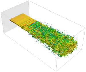
Large-scale instability modes being responsible for the breakup of a liquid sheet or jet under liquid injection in quiescent conditions have been documented in the literature. For instance, in the experimental work of Hoyt & Taylor (Reference Hoyt and Taylor1977), who considered high Reynolds number water jets issuing into still air, the jet was characterized initially by the growth of relatively small-scale modes driven by a shear instability. Further downstream, a much larger-scale mode developed, fragmenting the jet. Similar experimental findings have also appeared in the work of Wu & Faeth (Reference Wu and Faeth1995) and Crapper, Dombrowski & Pyott (Reference Crapper, Dombrowski and Pyott1975). More recently, via VoF simulations, Deshpande, Gurjar & Trujillo (Reference Deshpande, Gurjar and Trujillo2015) have shown that the fastest instability mode occurring at high-speed injection conditions is of such a small length scale that it is unable to displace the entire liquid core. Moving downstream, a much larger mode develops, breaking up the sheet. To illustrate this phenomenon more tangibly, VoF simulation results (described in § 4) of the sheet breakup under a stagnant environment are included in figure 1, which shows the development of the primary instability in the near field followed by the emergence of large-scale modes leading to the breakup of the sheet.

Figure 1. (a) Breakup of a liquid sheet injected into a stagnant air environment. (b) Side view of the development of the primary instability followed by the appearance of a large-scale sinuous mode. The inlet flow has a constant flat-hat profile without an imposed perturbation.
One of the aims of the present work is to analyse the conditions leading to the growth of these large-scale instabilities for liquid sheets injected into a still gas environment at high speed. To carry out this investigation, a spatial linear stability analysis is performed over a broad range of conditions, followed by VoF simulations. A key question is whether the dominant instability modes, which develop in the linear regime, continue to dominate as the process becomes nonlinear. As elaborated previously, this process has been analysed well under coflowing conditions but has yet to receive the same level of attention under a quiescent gas environment. A second aim is to identify the critical contributors to the growth of the observed large-scale modes, which is done via an energy analysis of the perturbation.
The paper is organized as follows. First, the linear stability analysis (LSA) and the associated results are presented in §§ 2 and 3, respectively. This is followed by a description of the VoF methodology at the beginning of §4, an account of the VoF simulation set-up in § 4.1, the evaluation of LSA assumptions in § 4.2, and the comparison of VoF and LSA predictions in §§ 4.3 and 4.4. We then extend the analysis into the nonlinear regime via VoF in § 5, to determine the fate of the fastest growing modes. An energy budget analysis identifying the sources responsible for the amplification of instabilities is presented in § 6, followed by a summary and conclusions in § 7.
2. Linear stability treatment
Often in LSA of two-phase flows, the approach consists of solving for the evolution of a perturbation, which is superimposed on a base flow profile (Boeck & Zaleski Reference Boeck and Zaleski2005; Fuster et al. Reference Fuster, Matas, Marty, Popinet, Hoepffner, Cartellier and Zaleski2013; Matas et al. Reference Matas, Delon and Cartellier2018). The adoption of this methodology can run into limitations when the base flow profile does not obey the governing equations exactly, but satisfies them only in an approximate sense. Additionally, for the types of problem considered here, which are motivated by fuel injection in engines and are therefore under high-speed conditions, it is not realistic to envision a base flow field that remains stable and steady. However, for much of the injection period, the flow fields in the near-field region of the injector nozzle are statistically stationary. Consequently, the mean fields within this statistically stationary or quasi-steady period can fulfil the role of the base flow field in LSA. It is in this spirit that we adopt a mean flow stability methodology in predicting the growth of disturbances. A detailed presentation of mean flow stability can be found in the works of Oberleithner, Rukes & Soria (Reference Oberleithner, Rukes and Soria2014) and Schmidt & Oberleithner (Reference Schmidt and Oberleithner2020).
The configuration of interest consists of a planar liquid sheet of thickness  $H$ injected into a quiescent gas at speed $U_{inj}$. The governing equations for mass and momentum are given, respectively, by
 $$\begin{gather} \boldsymbol{\nabla}\boldsymbol{\cdot} \boldsymbol{u} =0, \end{gather}$$
 $$\begin{gather}\frac{\partial\boldsymbol{u}}{\partial t} + \boldsymbol{u} \boldsymbol{\cdot} \boldsymbol{\nabla} \boldsymbol{u} =-\frac{1}{\rho}\,\boldsymbol{\nabla} p + \nu\,\nabla^2 \boldsymbol{u}. \end{gather}$$
 The density  $\rho$, and the dynamic and kinematic viscosities $\mu$ and $\nu$, are treated as constants in each thermodynamic phase. For the typical injection speeds and sheet thicknesses considered in the present work, $Fr^2$ is typically $O({10^5})$ or higher, thus gravitational effects can be ignored ( $Fr=U_{inj}/\sqrt {gH}$, i.e. Froude number). Even if a length scale pertaining to the onset of breakup is used, the value for $Fr^2$ is still much greater than 1, making the gravitational effects negligible.
In the present adoption of mean flow LSA treatment, rather than imposing the triple flow decomposition of the flow field (Oberleithner et al. Reference Oberleithner, Rukes and Soria2014; Schmidt & Oberleithner Reference Schmidt and Oberleithner2020), a Reynolds decomposition is used, where
 $$\begin{gather} \boldsymbol{u}(\boldsymbol{x},t) =\bar{\boldsymbol{u}}(\boldsymbol{x}) + \boldsymbol{u}'(\boldsymbol{x},t), \end{gather}$$
 $$\begin{gather}p(\boldsymbol{x},t) =\bar{p}(\boldsymbol{x},t) + p'(\boldsymbol{x},t). \end{gather}$$
Here, the overline denotes the time average within the quasi-steady-state period of liquid injection, and the prime indicates the respective fluctuating quantity.
Averaging the governing equations yields
 $$\begin{gather} \boldsymbol{\nabla}\boldsymbol{\cdot}\bar{\boldsymbol{u}} =0, \end{gather}$$
 $$\begin{gather}\frac{\partial\bar{\boldsymbol{u}}}{\partial t} + \bar{\boldsymbol{u}}\boldsymbol{\cdot}\boldsymbol{\nabla}\bar{\boldsymbol{u}} +\boldsymbol{\nabla}\boldsymbol{\cdot} (\overline{\boldsymbol{u}'\boldsymbol{u}'}) =-\frac{\boldsymbol{\nabla} \bar{p}}{\rho} + \nu\,{\nabla^2\bar{\boldsymbol{u}}}, \end{gather}$$
and by subtracting these two equations from (2.1), we obtain
 $$\begin{gather} \boldsymbol{\nabla}\boldsymbol{\cdot}(\boldsymbol{u}') =0, \end{gather}$$
 $$\begin{gather}\frac{\partial\boldsymbol{u}'}{\partial t} + \bar{\boldsymbol{u}}\boldsymbol{\cdot}\boldsymbol{\nabla}\boldsymbol{u}' + \boldsymbol{u}'\boldsymbol{\cdot}\boldsymbol{\nabla}\bar{\boldsymbol{u}} +\boldsymbol{\nabla}\boldsymbol{\cdot}(\boldsymbol{u}'\boldsymbol{u}' -\overline{\boldsymbol{u}'\boldsymbol{u}'}) =-\frac{\boldsymbol{\nabla} p'}{\rho} + \nu\,{\nabla^2\boldsymbol{u}'}. \end{gather}$$
Adopting a two-dimensional (2-D) dimensionality with  $\boldsymbol {u}=u(x,y,t)\,\boldsymbol {e}_x + v(x,y,t)\,\boldsymbol {e}_y$ and $p(x,y,t)$, where the streamwise, transverse and temporal coordinates are denoted by $(x,y,t)$, the momentum perturbation equation can be arranged as
 \begin{align} &
\frac{\partial\boldsymbol{u}'}{\partial t} +
\underbrace{\bar{u}\,\frac{\partial\boldsymbol{u}'}{\partial
x} +v'\,\frac{\partial\bar{\boldsymbol{u}}}{\partial y}
}_{{conventional\ advection}} +
\underbrace{\bar{v}\,\frac{\partial\boldsymbol{u}'}{\partial
y} }_{{transverse\ mean}} +
\underbrace{u'\,\frac{\partial\bar{\boldsymbol{u}}}{\partial
x} }_{{streamwise\ developing}} \nonumber\\
&\quad =-\frac{\boldsymbol{\nabla} p'}{\rho} +
\nu\,{\nabla^2\boldsymbol{u}'}
-\underbrace{\boldsymbol{\nabla}\boldsymbol{\cdot}(\boldsymbol{u}'\boldsymbol{u}'-\overline{\boldsymbol{u}'\boldsymbol{u}'})}_{{nonlinear}}.
\end{align}
\begin{align} &
\frac{\partial\boldsymbol{u}'}{\partial t} +
\underbrace{\bar{u}\,\frac{\partial\boldsymbol{u}'}{\partial
x} +v'\,\frac{\partial\bar{\boldsymbol{u}}}{\partial y}
}_{{conventional\ advection}} +
\underbrace{\bar{v}\,\frac{\partial\boldsymbol{u}'}{\partial
y} }_{{transverse\ mean}} +
\underbrace{u'\,\frac{\partial\bar{\boldsymbol{u}}}{\partial
x} }_{{streamwise\ developing}} \nonumber\\
&\quad =-\frac{\boldsymbol{\nabla} p'}{\rho} +
\nu\,{\nabla^2\boldsymbol{u}'}
-\underbrace{\boldsymbol{\nabla}\boldsymbol{\cdot}(\boldsymbol{u}'\boldsymbol{u}'-\overline{\boldsymbol{u}'\boldsymbol{u}'})}_{{nonlinear}}.
\end{align}The conventional advection term is the one that is typically employed in the traditional linear stability treatments (Schmid & Henningson Reference Schmid and Henningson2000; Criminale, Jackson & Joslin Reference Criminale, Jackson and Joslin2019). We assume that the transverse mean, streamwise developing and nonlinear terms are negligible. In § 4.2, it is shown that within a certain distance downstream of the inlet boundary, which depends on the type of instability considered, ignoring these additional advection terms is warranted. This space where these assumptions hold is referred to as the near-field region in the present work, where the LSA governing equations reduce to
 $$\begin{gather} \frac{\partial u'}{\partial x} + \frac{\partial v'}{\partial y} =0, \end{gather}$$
 $$\begin{gather}\frac{\partial u'}{\partial t} + \bar{u}\,\frac{\partial u'}{\partial x} + v'\,\frac{{\rm d}\bar{u}}{{\rm d}y} =-\frac{1}{\rho}\,\frac{\partial p'}{\partial x} + \nu \left(\frac{\partial^2}{\partial x^2}+\frac{\partial^2}{\partial y^2}\right) u', \end{gather}$$
 $$\begin{gather}\frac{\partial v'}{\partial t} + \bar{u}\,\frac{\partial v'}{\partial x} =-\frac{1}{\rho}\, \frac{\partial p'}{\partial y} + \nu \left(\frac{\partial^2}{\partial x^2} + \frac{\partial^2}{\partial y^2}\right)v' . \end{gather}$$
 It is understood implicitly that the field variables and physical properties take on values corresponding to the phase where they are being evaluated. For the mean flow fields, we impose the following profiles for  $\bar {\boldsymbol {u}}$:
 $$\begin{gather} \bar{\boldsymbol{u}} = [\bar{u},\bar{v}] = [\bar{u}(\kern0.7pt y), 0], \end{gather}$$
 $$\begin{gather}\bar{u}_L(\kern0.7pt y)=-K_1\,{\rm erf}\Bigl(\frac{y-H/2}{\delta_L} \Bigr)+K_2, \quad{}y\in[0,H/2], \end{gather}$$
 $$\begin{gather}\bar{u}_G(\kern0.7pt y)=-K_2\,{\rm erf}\Bigl(\frac{y-H/2}{\delta_G} \Bigl)\,+\,K_2, \quad{} y\in[H/2,W], \end{gather}$$
where  $K_1$ and $K_2$ are constants, $\delta$ is the shear layer thickness, and subscripts $L$ and $G$ indicate whether the quantity in question is liquid or gas. These error function profiles are used commonly in the literature (Yecko, Zaleski & Fullana Reference Yecko, Zaleski and Fullana2002; Boeck & Zaleski Reference Boeck and Zaleski2005; Schmidt & Oberleithner Reference Schmidt and Oberleithner2020), and as explained in § 4.1, they are imposed at the inlet boundary of VoF simulations. The extent to which the VoF predictions of mean velocity retain their expected form (2.8) throughout the computational domain is evaluated in § 4.2. Furthermore, we also have the continuity of shear stress of the mean flow field at the mean interface location $y=H/2$:
 \begin{equation} \mu_L\left.{\frac{\text{d}\bar{u}_L }{\text{d}y}}\right\vert_{y=H/2}=\mu_G\left.{\frac{\text{d}\bar{u}_G}{\text{d}y}}\right\vert_{y=H/2}. \end{equation}
How sharp this mean interface location remains as we move downstream is also evaluated in § 4.2. Equations (2.8) substituted into (2.9) and  $\bar {u}_L(\kern0.7pt y=0)=U_{inj}$ yield
 $$\begin{gather} K_1 = \frac{U_{inj}}{1 + \dfrac{\delta_G \mu_L}{\delta_L\mu_G}}, \end{gather}$$
 $$\begin{gather}K_2 = \frac{ U_{inj}}{ 1 + \dfrac{\delta_L \mu_G}{\delta_G\mu_L} }, \end{gather}$$
provided that  $H/(2\delta _L)\gtrsim 3$.
As illustrated in figure 2, the governing equations for the perturbations (2.7) are solved in a half-domain with  $y \in [0,W]$. By solving the problem in this fashion, the condition at the liquid centreline is varied depending on whether the perturbation mode is varicose or sinuous. Explicitly, the boundary conditions at the liquid centreline ( $y=0$) and at the gas boundary ( $y=W$) are
 $$\begin{gather} \text{varicose} \quad \left.\left[\frac{\partial u_L'}{\partial y}\right.\right\vert_{y=0}=0,\quad [v'\vphantom{\frac{d}{d}}\vert_{y=0}=0, \quad\left.\left[\frac{\partial p_L'}{\partial y}\right.\right\vert_{y=0}=0; \end{gather}$$
 $$\begin{gather}\text{sinuous}\quad [u_L'\vert_{y=0}=0,\quad \left.\left[\frac{\partial v_L'}{\partial y}\right.\right\vert_{y=0}=0,\quad [\,p_L'\vert_{y=0}=0; \end{gather}$$
 $$\begin{gather}\text{varicose and sinuous} \quad \left.\left[\frac{\partial u_G^{\prime}}{\partial y}\right.\right\vert_{y=W}=0,\quad [v_G'\vert_{y=W}=0,\quad \left.\left[\frac{\partial p_G'}{\partial y}\right.\right\vert_{y=W}=0. \end{gather}$$
The second set of auxiliary conditions is imposed at the gas–liquid interface and constitutes the interfacial constraints given by
 $$\begin{gather} \left.\left[-p_G^{\prime}+2\mu_G\,\frac{\partial v_G^{\prime}}{\partial y}\right.\right\vert_{y={H}/{2}} - \left.\left[-p_L^{\prime}+2\mu_L\,\frac{\partial v_L^{\prime}}{\partial y}\right.\right\vert_{y={H}/{2}} =- \gamma\,\frac{\partial^2 \eta}{\partial x^2}, \end{gather}$$
 $$\begin{gather}\mu_L \left.\left[\frac{\partial u_L^{\prime}}{\partial y} + \eta\,\frac{{\rm d}^2\bar{u}_L}{{{\rm d}y}^2} + \frac{\partial v_L^{\prime}}{\partial x}\right.\right\vert_{y={H}/{2}} = \mu_G \left.\left[\frac{\partial u_G^{\prime}}{\partial y} + \eta\, \frac{{\rm d}^2\bar{u}_G}{{{\rm d}y}^2} + \frac{\partial v_G^{\prime}}{\partial x}\right.\right\vert_{y={H}/{2}}, \end{gather}$$
 $$\begin{gather}\left.\left[\eta\,\frac{{\rm d}\bar{u}_L}{{\rm d}y}+u_L^{\prime}\right.\right\vert_{y={H}/{2}} = \left.\left[\eta\,\frac{{\rm d}\bar{u}_G}{{\rm d}y}+u_G^{\prime}\right.\right\vert_{y={H}/{2}}, \end{gather}$$
 $$\begin{gather}{}[v_L^{\prime}\vert_{y={H}/{2}} = [v_G^{\prime}\vert_{y={H}/{2}} \end{gather}$$
and
 \begin{equation} \frac{{\rm D}\eta}{{\rm D}t} = [v'_L\vert_{y={H}/{2}}, \end{equation}
where  $\gamma$ is the surface tension coefficient. Equations (2.12a) and (2.12b) represent the normal stress and shear stress balances. Continuity of horizontal and vertical velocities are given by (2.12c) and (2.12d). The interfacial displacement from the mean interfacial location ( $y=H/2$) is given by $\eta (x,t)$, as shown in figure 2, and the kinematic condition is given by (2.12e).

Figure 2. Schematic representation of the problem set-up, with (a) varicose perturbation and (b) sinuous perturbation. The flow is from left to right, and the nozzle orifice is located at  $x=0$.
To proceed with the calculation of perturbation growth rate, a normal mode decomposition is employed for treating the perturbations (Drazin & Reid Reference Drazin and Reid1981, p. 128):
 \begin{equation} [u'(x,y,t), v'(x,y,t), p'(x,y,t) ] =[\hat{u}(\kern0.7pt y), \hat{v}(\kern0.7pt y), \hat{p}(\kern0.7pt y) ] \exp[{\rm i}(kx-\omega t ) ], \end{equation}
where  $\hat {u}(\kern0.7pt y)$, $\hat {v}(\kern0.7pt y)$, $\hat {p}(\kern0.7pt y)$ are complex quantities, e.g. $\hat {u}(\kern0.7pt y)= \hat {u}_{R}(\kern0.7pt y)+{\rm i}\,\hat {u}_{I}(\kern0.7pt y)$. For the kinematic condition, the method of characteristics combined with the normal mode form can be used to obtain
 \begin{equation} \eta (x,t)= \hat{\eta} \exp[{\rm i}(kx-\omega t )], \quad \text{with}\ \hat{\eta} =\left.\left[\frac{\hat{v}_{(L,G)}}{{\rm i}kU_{(L,G)}-{\rm i}\omega}\right.\right\vert_{y={H}/{2}}. \end{equation}
Since we are dealing with a spatial instability analysis, the frequency is given by  $\omega =\omega _R\in \mathbb {R}$, and the wavenumber is given by $k=k_R+{\rm i}k_I\in \mathbb {C}$. The components $k_R$ and $k_I$ represent the wavenumber and the spatial growth rate of the perturbation, respectively.
The velocities and pressure are non-dimensionalized as
 \begin{equation} \tilde{U} =\frac{U}{U_{inj}}, \quad\tilde{u}=\frac{\hat{u}}{U_{inj}}, \quad\tilde{v}=\frac{\hat{v}}{U_{inj}}, \quad\tilde{p}=\frac{\hat{p}}{\rho_L U_{inj}^2}, \end{equation}
and similarly, the non-dimensional wavenumber and frequency are given by, respectively,
 \begin{equation} \tilde{k} = k H, \quad \tilde{\omega}=\frac{\omega H}{U_{inj}}. \end{equation}
In addition to the Weber number (1.1), two additional non-dimensional quantities appear in the analysis, namely the liquid-based Reynolds and Ohnesorge numbers,
 \begin{equation} Re_L=\frac{\rho_L U_{inj} H}{\mu_L} \quad\text{and}\quad Oh_L=\frac{\sqrt{2\, We_L}}{Re_L}. \end{equation}
The normal mode decomposition is substituted into the governing equations, boundary conditions and interfacial constraints, and a Chebyshev spectral representation is employed. The details of this procedure are included in the Appendix. The resulting final system that is solved is
 \begin{equation} \Bigl[\begin{array}{@{}cc@{}}
-\boldsymbol{C}_1 & -\boldsymbol{C}_0 \\ \boldsymbol{I} &
\boldsymbol{0} \end{array}\Bigr] \boldsymbol{\cdot}
\Bigl[\begin{array}{@{}c@{}} \tilde{k}\boldsymbol{a} \\ \boldsymbol{a}
\end{array}\Bigr] -\tilde{k} \Bigl[\begin{array}{@{}cc@{}} \boldsymbol{C}_2 &
\boldsymbol{0} \\ \boldsymbol{0} & \boldsymbol{I}
\end{array}\Bigr] \boldsymbol{\cdot} \Bigl[\begin{array}{@{}c@{}}
\tilde{k}\boldsymbol{a} \\ \boldsymbol{a} \end{array}\Bigr]
=\boldsymbol{0}, \end{equation}
\begin{equation} \Bigl[\begin{array}{@{}cc@{}}
-\boldsymbol{C}_1 & -\boldsymbol{C}_0 \\ \boldsymbol{I} &
\boldsymbol{0} \end{array}\Bigr] \boldsymbol{\cdot}
\Bigl[\begin{array}{@{}c@{}} \tilde{k}\boldsymbol{a} \\ \boldsymbol{a}
\end{array}\Bigr] -\tilde{k} \Bigl[\begin{array}{@{}cc@{}} \boldsymbol{C}_2 &
\boldsymbol{0} \\ \boldsymbol{0} & \boldsymbol{I}
\end{array}\Bigr] \boldsymbol{\cdot} \Bigl[\begin{array}{@{}c@{}}
\tilde{k}\boldsymbol{a} \\ \boldsymbol{a} \end{array}\Bigr]
=\boldsymbol{0}, \end{equation}
where the matrices  $\boldsymbol {C}_0$, $\boldsymbol {C}_1$ and $\boldsymbol {C}_2$ are the coefficient matrices pertaining to the governing equations, boundary conditions and interfacial relations. The eigenvector and eigenvalue being solved for in this generalized eigenvalue problem are, respectively, $\boldsymbol {a}=[\boldsymbol {a}_u^{L}, \boldsymbol {a}_v^{L}, \boldsymbol {a}_p^{L}, \boldsymbol {a}_u^{G}, \boldsymbol {a}_v^{G}, \boldsymbol {a}_p^{G}]^{\rm T}$ and $\tilde {k}$.
3. Linear stability predictions
As reported in the works of Marmottant & Villermaux (Reference Marmottant and Villermaux2004), Fuster et al. (Reference Fuster, Matas, Marty, Popinet, Hoepffner, Cartellier and Zaleski2013), Tammisola et al. (Reference Tammisola, Sasaki, Lundell, Matsubara and Söderberg2011) and Matas & Cartellier (Reference Matas and Cartellier2013) under a coflow configuration, the size of the shear layer thickness has a profound effect on the type of instability that develops. Hence, in the present work, which considers injection in quiescent conditions, the impact of shear layer thickness is examined in the gas ( $\delta _G$) and liquid ( $\delta _L$) phases. The nominal conditions considered are presented in table 1. The size $H$ is motivated by the orifice diameter of a commonly studied diesel type of injector, specifically the Engine Combustion Network Spray A nozzle (Engine Combustion Network, https://ecn.sandia.gov/). Some additional calculations have been performed (not shown) with different values of $W$ to examine the containment effect. The results have shown that the results presented here are independent of $W$, provided that $W$ is equal to at least $10H$.
Table 1. Physical properties of fluids and key non-dimensional quantities used in LSA and VoF predictions, along with the nominal values for operating parameters.

First, predictions of spatial growth rate ( $-\tilde {k}_I$) for both varicose and sinuous modes are plotted as a function of wavenumber, $\tilde {k}_R$, in figure 3. The six plots in the figure correspond to different values of $\delta _G/H$, ranging from $1/10$ to 1, while liquid shear layer thickness is held constant at $\delta _L=H/12$. At low values of $\delta _G/H$, i.e. for $\delta _G/H\sim O({10^{-1}})$, the peak in these dispersion curves is located at $\tilde {k}_R=kH\approx 15$, which implies that the length scale of the fastest growing mode is significantly smaller than $H$. As such, it is expected that these instabilities leave the inner core of the liquid sheet largely intact, and that their direct effect is a disruption limited to the sheet's surface. Beginning at approximately $\delta _G/H=1/6$, a second peak develops at $\tilde {k}_R\approx 1$ for the sinuous mode. With larger values for the gas shear layer thickness, this second peak becomes progressively more dominant, and at $\delta _G/H=1.0$, it is growing three times faster than the secondary peak.

Figure 3. Spatial growth rate versus wavenumber for different gas shear layer thicknesses: (a)  $\delta _G/H =1/10$, (b) $\delta _G/H =1/8$, (c) $\delta _G/H =1/6$, (d) $\delta _G/H =1/4$, (e) $\delta _G/H =1/2$ and (f) $\delta _G/H =1$. Conditions pertain to those listed in table 1. A new peak is observed at lower wavenumbers (higher wavelengths), which becomes dominant at $\delta _G/H=1/6$.
The appearance of a dominant second peak with larger  $\delta _G$ exists only for the sinuous mode. For the varicose mode, the fastest growing mode remains in the much larger wavenumber range. In fact, both sinuous and varicose mode predictions are almost indistinguishable, with the exception of the lower wavenumber range, i.e. $\tilde {k}_R\lesssim 2$. In this part of the wavenumber space, the sinuous growth rate deviates strongly from the varicose mode by manifesting much more significant growth. Since the associated length scale of this mode is comparable to or larger than $H$, its growth will lead ultimately to the total disruption of the sheet, provided that it survives beyond the linear regime. This behaviour is tested with the VoF simulations presented in § 5.
To examine the effect of  $\delta _L$, the previous calculations are repeated under the same conditions and fluid properties employed for the gas shear layer examination, but with $\delta _G$ fixed at $H/10$. The associated spatial growth rate curves are presented in figure 4, where $\delta _L/H$ ranges from $H/12$ to $H/4$. Unlike the previous predictions for the gas shear layer thickness, the growth rate curves remain almost the same as $\delta _L$ is varied for both varicose and sinuous modes. These results indicate that, at least within the linear regime of instability evolution, the liquid-based shear layer thickness has a negligible effect. Specifically, when we consider the fastest growing mode, the change in the corresponding wavenumber is less than $4\,\%$ when $\delta _L$ is varied from $H/12$ to $H/4$.

Figure 4. Spatial growth rate versus wavenumber for different liquid shear layer thicknesses corresponding to (a) varicose mode and (b) sinuous mode. Conditions pertain to those listed in table 1 with  $\delta _G/H=1/10$.
The results shown in figure 4 lie in stark contrast to those presented by Turner et al. (Reference Turner, Healey, Sazhin and Piazzesi2011), who report that the size of the shear layer in the denser fluid, i.e. the liquid, has the most significant effect on the growth rate of the disturbances. A closer look at the differences between their approach and the present work reveals that, most likely, the inviscid treatment (Rayleigh equation) and linear base profiles employed by Turner et al. (Reference Turner, Healey, Sazhin and Piazzesi2011) are the contributing factors to the observed discrepancy. In our case, the viscous contribution is accounted for by the solution of the Orr–Sommerfeld system, along with the imposition of the full set of interfacial constraints. Compared to an inviscid treatment, the continuity of horizontal velocity and the shear stress condition are of particular significance. The argument made in Turner et al. (Reference Turner, Healey, Sazhin and Piazzesi2011) is that with  $Re_L\sim O ({10^4})$, the viscous term can be neglected. While that may hold true for the base or mean velocities, the perturbation velocities have extremely sharp gradients at the interface (this is shown in a later section, specifically in figure 24); hence neglecting their associated viscous contribution is questionable.
The associated phase velocities  $c_p=U_{inj}\tilde {\omega }_R/\tilde {k}_R$ and group velocities $c_g=U_{inj}\,\partial \tilde {\omega }_R/\partial \tilde {k}_R$ are plotted in figure 5, corresponding to the two extreme values of $\delta _G/H$, i.e. $\delta _G/H=1/10$ and $1$. Deviations of both $c_p$ and $c_g$ from the injection speed $U_{inj}$ are noticeably more pronounced for low wavenumbers, and this deviation corresponds, for the most part, to a slower propagation of the disturbances. This effect is more significant for $\delta _G/H=1$, and the wavenumber range where it occurs matches where the large-scale mode is detected for the sinuous mode. Indeed, it is the sinuous mode where the largest discrepancies from $U_{inj}$ occur for the phase and group velocities. For the varicose mode at $\delta _G/H=1$, all disturbances travel almost uniformly at $U_{inj}$. Even at $\delta _G/H=1/10$, the varicose mode travels mostly with 10 % of the injection speed.

Figure 5. Phase velocities versus wavenumber for varicose and sinuous modes corresponding to (a)  $\delta _G/H=1/10$ and (b) $\delta _G/H=1$. Group velocities versus wavenumber for varicose and sinuous modes corresponding to (c) $\delta _G/H=1/10$ and (d) $\delta _G/H=1$. Conditions pertain to those listed in table 1.
To examine whether the development of the large-scale sinuous mode occurs under a broader range of conditions, a number of additional cases are examined, as documented in table 2. The wavenumbers  $k_{R,crit}$, corresponding to the critical or fastest growing mode for each of these cases, are extracted. The associated wavelengths $\lambda _{crit} (=2{\rm \pi} /k_{R,crit})$ are plotted in figure 6 for the sinuous mode, and in figure 7 for the varicose mode, as a function of the gas shear layer thickness. For the varicose case, $\lambda _{crit,varicose}/H$ increases monotonically with $\delta _G/H$, i.e. $\lambda _{crit,varicose}/H \sim (\delta _G/H)^{P}$, where $P$ varies between $0.54$ to $0.64$ for all curves.
Table 2. Additional high-speed injection cases examined under LSA. With the exception of a variable surface tension, the physical properties are the same as those listed in table 1.


Figure 6. Predicted critical wavelengths from LSA corresponding to the sinuous mode.

Figure 7. Predicted critical wavelengths from LSA corresponding to the varicose mode.
In contrast, for the sinuous modes, beyond a value of  $\delta _G/H$ ranging between 0.15 and 0.3, all curves collapse onto a single curve irrespective of $Re_L$ and $Oh_L$, namely
 \begin{equation} \frac{\lambda_{crit,sinuous}}{H} = 14.26\Bigl(\frac{\delta_G}{H}\Bigr)^{0.766}, \quad \delta_G/H \gtrsim 0.3. \end{equation}
This hints at a potential universality of the scaling of the critical wavelength with gas shear layer thickness for  $\delta _G/H \gtrsim 0.3$. This collapse is accompanied by an abrupt change in the magnitude of $\lambda _{crit,sinuous}/H$, which increases by at least one order of magnitude as the maximum growth rate shifts from the high wavenumber region to the lower wavenumber range.
For smaller values of  $\delta _G/H$ as shown in figure 6, i.e. $\delta _G/H\lesssim$0.1, the critical sinuous mode wavelengths still scale with $\delta _G/H$, i.e. $\lambda _{crit,sinuous}/H\sim (\delta _G/H)^{P}$, where $P$ varies between $0.54$ and $0.64$. However, the collapse of all curves observed for $\delta _G/H\gtrsim 0.3$ is absent since each curve is distinct and varies depending on the associated values for $Re_L$ and $Oh_L$. Specifically, $\lambda _{crit,sinuous}/H$ decreases with increasing $Re_L$ or increasing $Oh_L$. A transition region exists in the range $0.1\lesssim \delta _G/H \lesssim 0.3$, where $\lambda _{crit}/H=f(\delta _G/H; Oh_L, Re_L)$ merges from a multi-valued function to practically a single-valued function with respect to the gas shear layer thickness.
To examine whether the dominant large-scale sinuous mode exists also at lower injection speeds, two additional cases are considered. The first is at  $U_{inj}=10\ {\rm m}\ {\rm s}^{-1}$ ( $Re_L=1295$ and $Oh_L=0.013$), and the second is at $U_{inj}=5\ {\rm m}\ {\rm s}^{-1}$ ( $Re_L=647$ and $Oh_L=0.013$), with all fluid properties and $H$ remaining the same. The resulting dispersion relations are plotted in figures 8 and 9 as functions of $\delta _G/H$.

Figure 8. Spatial growth rate versus wavenumber for milder injection cases, for (a)  $\delta _G/H=1/10$, (b) $\delta _G/H=1/8$, (c) $\delta _G/H=1/6$, (d) $\delta _G/H=1/4$, (e) $\delta _G/H=1/2$, and (f) $\delta _G/H=1$ (with $U_{inj}= 10\ {\rm m}\ {\rm s}^{-1}$, $Re_L=1295$, $Oh_L=0.0134$).

Figure 9. Spatial growth rate versus wavenumber for milder injection cases, for (a)  $\delta _G/H=1/10$, (b) $\delta _G/H=1/8$, (c) $\delta _G/H=1/6$, (d) $\delta _G/H=1/4$, (e) $\delta _G/H=1/2$ and (f) $\delta _G/H=1$ (with $U_{inj}= 5\ {\rm m}\ {\rm s}^{-1}$, $Re_L=647$, $Oh_L=0.0134$).
As opposed to the double-peak behaviour observed for  $\delta _G/H\gtrsim 1/10$ (consider figure 3), the growth rates at these lower injection speed cases have a single peak. This implies that as the shear layer increases, the abrupt change in critical wavelength by one order of magnitude observed previously is absent under milder injection conditions. A second observation is that the range of wavenumbers where the growth rate is non-negligible is much smaller when compared to the growth rate curves under high-speed conditions. There are no peaks or even positive growth rates at high wavenumbers. In fact, $\lambda _{crit,sinuous}/H$ and $\lambda _{crit,varicose}/H$ are $O\left ({1}\right )$ for both lower velocity cases over the range of shear layer thickness considered.
4. Volume-of-fluid simulations
Capturing the full nonlinear dynamics of the perturbation process leading to the sheet breakup is done in the present investigation using a VoF methodology (Tryggvason, Scardovelli & Zaleski Reference Tryggvason, Scardovelli and Zaleski2011). The particular flavour of the VoF method employed in the present study consists of an algebraic VoF solver phibasedFoam (Agarwal, Ananth & Trujillo Reference Agarwal, Ananth and Trujillo2022). This solver is a slightly modified version of the interFoam code, which is part of the OpenFoam open source distribution of continuum mechanics solvers (OpenFoam foundation, https://openfoam.org/). The discretization of the governing equations is done via finite volume. The solver begins with the evolution of  $\alpha$, which is the fraction of liquid that occupies a given computational cell. This evolution is obtained from the solution of
 \begin{equation} \frac{\partial \alpha}{\partial t} + \boldsymbol{\nabla}\boldsymbol{\cdot}(\boldsymbol{u}\alpha) =0. \end{equation}
To mitigate the effects of numerical diffusion of  $\alpha$ due to its sharpness, the VoF scheme employs a compressive interface capturing methodology advanced by Ubbink & Issa (Reference Ubbink and Issa1999) and Rusche (Reference Rusche2003), with contributions from Henry Weller. Subsequently, the following two-phase momentum equation is solved:
 \begin{equation} \frac{\partial (\rho\boldsymbol{u})}{\partial t} +\boldsymbol{\nabla}\boldsymbol{\cdot}(\rho\boldsymbol{u}\boldsymbol{u}) =-\boldsymbol{\nabla} p + \boldsymbol{\nabla}\boldsymbol{\cdot}(\mu\,\boldsymbol{\nabla}\boldsymbol{u}) + \boldsymbol{\nabla}\boldsymbol{u}\boldsymbol{\cdot}\boldsymbol{\nabla}\mu + \rho\boldsymbol{g} + \sigma\kappa\,\boldsymbol{\nabla}\alpha, \end{equation}
where the solenoidal condition of the velocity field has been used to expand the divergence of the stress tensor. The density and viscosity are obtain from  $\rho =\rho _L\alpha + \rho _G(1-\alpha )$ and $\mu =\mu _L\alpha +\mu _G(1-\alpha )$ (Deshpande, Anumolu & Trujillo Reference Deshpande, Anumolu and Trujillo2012). The last term on the right-hand side is the surface tension term based on the continuum surface force method (Brackbill, Kothe & Zemach Reference Brackbill, Kothe and Zemach1992), where $\sigma$ is the surface tension coefficient, and $\kappa$ is the interface curvature defined as $\kappa = -\boldsymbol {\nabla }\boldsymbol {\cdot }{[\boldsymbol {n}_{\varGamma }]}$. Here, $\boldsymbol {n}_{\varGamma }$ is the interface normal unit vector, given by $\boldsymbol {n}_{\varGamma }=\boldsymbol {\nabla }\alpha /(\lvert {\boldsymbol {\nabla }\alpha }\rvert )$. The prediction of velocity is followed by the solution of a pressure Poisson system with variable coefficients and a velocity corrector step. A description of the interFoam algorithm, along with an evaluation of its performance considering the various aspects of the two-phase flow solution, is provided in Deshpande et al. (Reference Deshpande, Anumolu and Trujillo2012).
A reported notable weakness in interFoam is the prediction of interfacial curvature, which is fundamental in the calculation of surface tension. To remedy this difficulty, phibasedFoam implements an improved curvature estimation by solving for a signed distance function  $\phi _{dis}$ within the interfacial region coupled to the solution of the Hamilton–Jacobi equation away from this region. Based on this procedure, the predictions of curvature and the numerical convergence rate are improved noticeably. These improvements are much more substantial for cases that are either completely or heavily surface tension dominated. For the cases considered in the present work, which occur at much higher $We_L$ values, we found that the differences were negligible in comparison to the standard interFoam.
4.1. Volume-of-fluid domain and initialization
Except for the calculations shown in figure 1, all the VoF computations presented in the paper are 2-D, allowing for much better resolution of the interfacial region. This is needed particularly for high-speed injection, where the perturbation eigenvectors become extremely sharp at the interface, requiring sub-micron resolution. Carrying out these calculations in three dimensions, where these perturbations are fully resolved numerically, poses a significant computational expense, especially in the calculation of statistical quantities, which require a sufficiently long time window. Additionally, since much of the focus of the work is on the initial development of instabilities, which are 2-D in nature, limiting the VoF simulations to two dimensions is reasonable.
The computational domain for the VoF calculation consists of a rectangular region having height  $20H$ and length $100H$, as shown in figure 10. This figure shows the varying levels of resolution $\Delta x$ employed in different parts of the domain. Throughout the inlet region, grid size $\Delta x=0.375\ \mathrm {\mu } {\rm m}$ is used, which is sufficiently fine to resolve the perturbation velocities and perturbation pressure. As we move away from this region, the grid employed becomes progressively more coarse, and far away from the location of interest, the resolution is $\Delta x=6\ \mathrm {\mu } {\rm m}$.

Figure 10. Depiction of the VoF domain employed in liquid sheet breakup simulations, along with the associated mesh resolution. The close-up view of the inlet provides details of the imposed velocity profile (4.6).
The velocity profile imposed at the inlet is given by
 $$\begin{gather} u(x=0,y,t) = \bar{u}(\kern0.7pt y) + u^{\prime}(x=0,y,t), \end{gather}$$
 $$\begin{gather}v(x=0,y,t) = v^{\prime}(x=0,y,t), \end{gather}$$
where mean velocities are given in (2.8), and the perturbation velocities adopt a normal mode form (2.13), namely
 $$\begin{gather} u'(0,y,t) = {\rm Re} \left[ [\hat{u}_{R}(\kern0.7pt y) + {\rm i}\,\hat{u}_{I}(\kern0.7pt y)][\cos(kx-\omega_R t) +{\rm i}\sin(kx-\omega_R t)] \right|_{x=0}, \end{gather}$$
 $$\begin{gather}v'(0,y,t) = {\rm Re} \left[ [\hat{v}_{R}(\kern0.7pt y) + {\rm i}\,\hat{v}_{I}(\kern0.7pt y)][\cos(kx-\omega_R t) +{\rm i}\sin(kx-\omega_R t)] \right|_{x=0}. \end{gather}$$
Here,  ${\rm Re}$ denotes the extraction of the real part of a complex expression. Substituting these expressions into (4.3) gives
 \begin{align} &u(x=0,y,t)\nonumber\\&\quad =\begin{cases} -K_1\,{\rm erf}\begin{pmatrix}\dfrac{y-\dfrac{H}{2}}{\delta_L}\end{pmatrix}+K_2+\hat{u}_{L,R}(\kern0.7pty)\cos\left(\omega_R t\right)+\hat{u}_{L,I}(\kern0.7pty)\sin\left(\omega_R t\right), & 0<y<\dfrac{H}{2},\\ -K_2\,{\rm erf}\begin{pmatrix}\dfrac{y-\dfrac{H}{2}}{\delta_G}\end{pmatrix}+K_2+\hat{u}_{G,R}(\kern0.7pty)\cos(\omega_R t)+\hat{u}_{G,I}(\kern0.7pt y)\sin(\omega_Rt), & \dfrac{H}{2}< y< W,\\K_1\,{\rm erf}\begin{pmatrix}\dfrac{y+\dfrac{H}{2}}{\delta_L}\end{pmatrix}+K_2+\hat{u}_{L,R}(\kern0.7pty)\cos(\omega_R t)+\hat{u}_{L,I}(\kern0.7pt y)\sin(\omega_Rt), & -\dfrac{H}{2}< y<0,\\K_2\,{\rm erf}\begin{pmatrix}\dfrac{y+\dfrac{H}{2}}{\delta_G}\end{pmatrix}+K_2+\hat{u}_{G,R}(\kern0.7pty)\cos(\omega_R t)+\hat{u}_{G,I}(\kern0.7pt y)\sin(\omega_Rt), & -W< y<-\dfrac{H}{2}, \end{cases}\end{align}
 \begin{align} v(x=0,y,t) = \begin{cases} \hat{v}_{L,R}(\kern0.7pt y)\cos\,(\omega_R t)+\hat{v}_{L,I}(\kern0.7pt y)\sin\, (\omega_R t), & 0< y<\dfrac{H}{2},\\ \hat{v}_{G,R}(\kern0.7pt y)\cos\,(\omega_R t)+\hat{v}_{G,I}(\kern0.7pt y)\sin\,(\omega_R t), & \dfrac{H}{2}< y< W,\\ \hat{v}_{L,R}(\kern0.7pt y)\cos\,(\omega_R t)+\hat{v}_{L,I}(\kern0.7pt y)\sin\,(\omega_R t), & -\dfrac{H}{2}< y<0,\\ \hat{v}_{G,R}(\kern0.7pt y)\cos\,(\omega_R t)+\hat{v}_{G,I}(\kern0.7pt y)\sin\,(\omega_R t), & -W< y<-\dfrac{H}{2}. \end{cases} \end{align}
The imposed perturbations at the inlet are ensured to be small by having the interfacial displacement  $\hat {\eta }$, which is obtained from (2.14), to be $1.5\,\%$ of the liquid sheet thickness $H$.
$H$.
The VoF simulations are initiated by imposing the velocity profiles of (4.6) on the inlet boundary as depicted in figure 10. This applies to both the liquid and gas phase portions of the inlet boundary. For example, a simulation of liquid sheet injection under conditions listed in table 1, and with a superimposed sinuous mode, is shown in figure 11. In figure 11(a), the sheet is captured during its initial injection period or initial transient, and in figure 11(b), the sheet resides within the quasi-steady-state period. Velocity time histories at various  $x$ locations and at $y=H/2$ are also shown in figure 11(c). These histories show that the initial transient caused by the passage of the sheet tip is recorded at progressively longer times with increasing distance from the inlet location. Beyond $tU_{inj}/H=111$, as indicated by the red dashed line in figure 11(c), it is safe to assume that we have entered a quasi-steady state, and VoF data are collected only within this time period, i.e. not during the initial transient. This reference time $tU_{inj}/H=111$ also holds for other excitation frequencies $\tilde {\omega }_R$ of the sinuous mode pertaining to the nominal conditions of table 1. Regarding the varicose mode, the physical domain of interest is much shorter, as discussed in § 4.2. Therefore, the quasi-steady period is achieved more quickly, which implies that the reference initial time $tU_{inj}/H=111$ is more than sufficient.

Figure 11. Example of a VoF simulation corresponding to the critical sinuous mode (table 1,  $\tilde {\omega }_R=0.3064$ and $\delta _G/H=1$) at (a) $tU_{inj}/H=33.33$, (b) $tU_{inj}/H=222.22$, along with velocity time histories of probes located at various streamwise locations and at $y=H/2$.
4.2. Validity of LSA assumptions
With the use of the VoF simulations, the various assumptions employed in the LSA can be examined. This entails the examination of both mean quantities as well as the various advection terms discarded in the perturbation equation (2.6). The VoF simulations are time-averaged from  $tU_{inj}/H=111$ to $tU_{inj}/H$ ranging from 222.2 to 666.67, depending on the type of instability being considered. This comprises a sufficient time period to obtain statistically converged quantities within the domain $0\leqslant x/H\leqslant 20$. Results corresponding to the sinuous and varicose modes are shown in figure 12. Both of these modes pertain to their respective critical condition, where the excitation frequency results in the peak growth rate predicted from linear stability. Here, the sinuous mode corresponds to $\delta _G/H=1$, and the varicose mode to $\delta _G/H=1/6$. This provides a sufficient range in the wavelengths of the perturbations observed.

Figure 12. Average streamwise velocity for (a) the sinusoidal mode and (b) the varicose mode; average transverse velocity for (c) the sinusoidal mode and (d) the varicose mode; and average liquid fraction profiles for (e) the sinusoidal mode and (f) the varicose modes. The sinuous and varicose mode calculations correspond to their critical quantities, and the associated gas shear layer thicknesses used in the calculations are respectively  $\delta _G/H=1$ and $\delta _G/H=1/6$. The operating parameters are those listed in table 1.
Beginning with the streamwise mean velocity, the assumption made is that it conforms to an error function (2.8), and that this profile remains constant as we move downstream. Results shown in figure 12(a) confirm this behaviour, where  $\bar{u}/U_{inj}$ remains unchanged up to $x=10H$, and begins to deviate slightly from the error function at $x=15H$. Even at $x=20H$, the profile retains its initial shape, but some slight smoothing takes place at approximately $y=\pm H/2$, i.e. the interfacial region. For the varicose mode, due to its much smaller wavelength, deviations from the error function profile happen sooner, as plotted in figure 12(b). Also, the deviations are concentrated in a narrower band around the interface, where the growth of small lumps is detected. Up to $x=2H$, the mean streamwise velocity stays essentially unchanged, and this corresponds to approximately three wavelengths of the varicose mode. By $x=4H$, there is a noticeable protrusion at the interface, while the rest of the velocity profile retains its original error function form. This means that predictions from LSA are likely to have difficulties for this mode beyond approximately $x=4H$.
Regarding the transverse velocity, the time-averaged VoF data are shown in figure 12(c) for the sinuous mode and in figure 12(d) for the varicose mode. As given in (2.8), it is expected that both of these quantities should remain equal to zero. The results show that this was accomplished well for the sinuous mode up to  $x=20H$, with increasing levels of discrepancy with progressively longer distances from the inlet boundary. For the varicose mode, the approximation holds again in a much shorter range, and in comparison to the sinuous mode, the discrepancy is more significant. Nevertheless, its maximum value is approximately 2 % of $U_{inj}$, which is still relatively small.
Finally, the mean liquid fraction fields are shown in figures 12(e) and 12(f) for the sinuous and varicose modes, respectively. Within the domain of interest, which extends up to  $20H$ for the sinuous mode and $4H$ for the varicose mode, the varicose mode better retains its initial shape. Beyond $x=10H$, the sinuous mode exhibits a noticeable degree of smoothing. This has an impact on the interfacial constraints in LSA, which are based on a departure $\eta$ from the undisturbed interface location, i.e. $y=H/2$. Since beyond $x=10H$ or worse, $x=15H$, the interface is diffused over a larger band around $y=H/2$, and this implies a higher level of uncertainty in identifying the interface location, which is expected to have consequences in the calculation of interfacial constraints. However, below $x=10H$, the degree of interface diffusion is relatively mild, and the interfacial region is sharp.
In conclusion, the findings depicted in figure 12 concerning mean quantities show that the assumptions inherent in LSA are valid for the sinuous mode up to  $x=10H$ or even perhaps $x=15H$ for $\delta _G/H=1$, while for the varicose mode, the domain of validity extends up to approximately $x=3H$ for $\delta _G/H=1/6$. In a more general sense, considering the ranges in $\delta _G/H$ employed in the present work, the range of validity is approximately $x=6H$ to $x=15H$ for the sinuous mode, and $x=2H$ to $x=15H$ for the varicose mode.
Turning our attention to the discarded terms in the perturbation evolution equation (2.6), we have the transverse mean, streamwise developing and the nonlinear term. Via VoF calculations, we can calculate these neglected terms and compare their magnitudes to the magnitude of the retained conventional advection term. If these discarded terms can be shown to have a much lower magnitude than the conventional term over some range in  $x/H$, then their omission is justified.
To get a sense of the magnitude and the general structure of each of the advection terms, image plots of their instantaneous values within the near-field region are shown in figures 13 and 14 for the sinuous and varicose modes, respectively. A log scale is used to indicate their magnitude. First, the conventional term is significantly higher by orders of magnitude than the streamwise developing and transverse mean advection. It is actually the nonlinear contribution that competes more closely with the conventional advection term, but even this nonlinearity is at least an order of magnitude smaller. The results also show that the largest magnitude is concentrated in the interfacial region. Away from this region, there are errant droplets, which are remnants of the initial transient, that give the advection fields some degree of structure. This is apparent mostly for  $\lvert {y}\rvert \gtrsim 2H$. Regarding the varicose mode, the same observation holds, with the exception that the shape of the interface is understandably different.

Figure 13. Instantaneous image plots at  $tU_{inj}/H=666.66$ of the various advection terms (absolute values) in the near field for the critical sinuous mode with $\delta _G/H=1$ under conditions listed in table 1: (a) $|\bar {u}\,\partial \boldsymbol {u}'/\partial x + v'\,\partial \bar {\boldsymbol {u}}/\partial y|$, (b) $|\bar {v}\,\partial \boldsymbol {u}'/\partial y|$, (c) $|u'\,\partial \bar {\boldsymbol {u}}/\partial x|$, (d) $|\boldsymbol {\nabla } \boldsymbol {\cdot } (\boldsymbol {u}'\boldsymbol {u}'-\overline {\boldsymbol {u}'\boldsymbol {u}'})|$.

Figure 14. Instantaneous image plots at  $tU_{inj}/H=555.55$ of the various advection terms (absolute values) in the near field for the critical varicose mode with $\delta _G/H=1/6$ under conditions listed in table 1: (a) $|\bar {u}\,\partial \boldsymbol {u}'/\partial x + v'\,\partial \bar {\boldsymbol {u}}/\partial y|$, (b) $|\bar {v}\,\partial \boldsymbol {u}'/\partial y|$, (c) $|u'\,\partial \bar {\boldsymbol {u}}/\partial x|$, (d) $|\boldsymbol {\nabla } \boldsymbol {\cdot } (\boldsymbol {u}'\boldsymbol {u}'-\overline {\boldsymbol {u}'\boldsymbol {u}'})|$.
To gain a quantitative evaluation of the magnitude of the advection terms, a time average is taken of their absolute value as a function of  $x/H$ at $y=H/2$. As noted previously, this coincides with the undisturbed interface location. Since the advection terms pertain to fluctuating quantities, the absolute value is used in the time average. Otherwise, the time average naturally leads to progressively smaller values tending towards zero as the averaging period increases. The results are shown in figure 15 for both critical sinuous and varicose modes.

Figure 15. Time average of the absolute value of the various advection terms calculated under conditions listed in table 1: (a) terms corresponding to the critical sinuous mode with  $\delta _G/H=1$; (b) terms corresponding to the critical varicose mode with $\delta _G/H=1/6$.
For the sinuous mode, shown in figure 15(a), the conventional advection term is two to three orders of magnitude larger than their counterpart transverse mean and streamwise developing terms. The nonlinear term more closely approaches the magnitude of the conventional term, and the gap between these two decreases with increasing  $x/H$ as the nonlinearities grow in strength. For the varicose mode shown in figure 15(b), the difference between the conventional advection term and its counterparts is even larger, being approximately two to four orders of magnitude. Again, the nonlinear term is the largest discarded term, and the gap between it and the conventional term lessens as we move downstream from the inlet boundary. In summary, the assumption of only retaining the conventional advection term within the near field is warranted by the results from VoF simulations.
4.3. Extracting growth rates from VoF
To compare VoF and LSA predictions, perturbation growth rates are employed. Our approach for calculating these growth rates from VoF simulations is based on a procedure presented by Schmidt & Oberleithner (Reference Schmidt and Oberleithner2020). It employs the kinematic relationship (2.12e), which is used to link the interface displacement with the normal perturbation velocity, namely,
 \begin{equation} \eta(x,t) = \frac{v_L'(x,y=H/2,t)}{{\rm i}\,(k\,U_L(\kern0.7pt y=H/2) -\omega)}. \end{equation}
The disturbed normal velocity is obtained in the VoF simulations by probing it at the undisturbed location  $(x,y=H/2)$. The time series of $v'(x,H/2,t)$ can be Fourier decomposed as
 \begin{equation} v'(x,H/2,t) = \sum_{n\neq 0} A_n(x,y=H/2) \exp({\rm i}\omega_n t), \end{equation}
where  $\omega _n$ is the frequency of the $n{\rm th}$ Fourier mode and $A_n$ is the corresponding amplitude. In the calculation of growth rate, only the fundamental mode ( $n=1$) is considered, and the extraction of $v'(x,H/2,t)$ data is extended only within a relatively small distance in the $x$ direction, guaranteeing that the presence of other modes is negligible. Employing the normal mode decomposition, we have
 \begin{equation} v'(x,H/2,t)=\hat{v}(H/2)\exp(-k_I x)\exp[{\rm i}(k_Rx-\omega t)], \end{equation}
where  $k=k_R+{\rm i}k_I$. Considering only the fundamental mode and only the amplitude of both previous equations yields
 \begin{equation} A_1(x,y=H/2)= \hat{v}(H/2)\exp(-k_I x). \end{equation}
This can be repeated at some other position downstream of  $x$; for instance,
 \begin{equation} A_1(x+\Delta x,y=H/2)= \hat{v}(H/2)\exp(-k_I [x+\Delta x]). \end{equation}
Taking the ratio of both equations above, and taking the limit as  $\Delta x\rightarrow 0$, we obtain
 \begin{equation} -k_I=\lim_{\Delta x\rightarrow 0} \left[ \frac{\ln A_1(x+\Delta x,y=H/2) -\ln A_1(x,y=H/2)}{\Delta x} \right] =\frac{{\rm d}}{{\rm d}\kern0.06em x}(\ln(A_1)), \end{equation}
which is the expression employed in the calculation of growth rate  $-k_I$ from VoF data.
4.4. Comparison between linear stability and VoF
An examination of whether the predictions originating from the spatial LSA agree with the full Navier–Stokes treatment provided by the VoF is presented in this subsection. The nominal conditions pertaining to table 1 are chosen. Other VoF calculations performed at  $Re_L=25\,910$ and $Oh_L=0.066$ have led to a similar agreement with LSA predictions but are excluded here for the sake of brevity. We consider two cases corresponding to the critical sinuous and varicose modes, and examine their behaviour as a function of gas shear layer thickness. The VoF calculations employ the inlet flow conditions described in (4.6), and the data are obtained in the quasi-steady-state period, as commented earlier.
Example VoF results are shown in figure 16 for both modes, where a notable difference in perturbation length scale is clearly apparent. The sinuous mode has a wavelength that is approximately an order of magnitude longer than the varicose mode. In addition, some degree of surface breakup is observed for both cases towards the outflow face of the observation window as the perturbation grows.

Figure 16. VoF simulation results for  $\delta _G/H=1/4$ corresponding to the critical (a) sinuous mode and (b) varicose mode. The distance from the inlet is displayed in terms of liquid sheet thickness $H$.
$H$.
Quantitatively, the comparison between LSA predictions and VoF simulations is shown in figure 17 for the sinuous mode, and in figure 18 for the varicose mode, as functions of distance from the inlet. As we saw previously, in § 4.2, we consider only the near-field region, where the assumptions of linearity in LSA, mean profiles, and the exclusion of additional advection terms are reasonable. With decreasing gas shear layer thickness  $\delta _G$, the critical growth rate for both modes increases, leading to a faster manifestation of nonlinear effects. Consequently, the extent of the longitudinal domain shown in figures 17 and 18 is smaller with decreasing $\delta _G$. For the critical varicose mode, shown in figure 18, the differences with VoF results are more noticeable. We speculate that this is due to a more significant departure from the assumed form of the mean velocity fields (2.8) as a function of $x$, which is more prevalent in the varicose case as depicted in figure 12. Nevertheless, there is good agreement overall between LSA and VoF in the near field.

Figure 17. The VoF data corresponding to sinuous mode simulations and associated exponential curve fits (VoF fit). The respective values for gas shear layer thickness ( $\delta _G/H$) and growth rate predictions from LSA are: (a) $\delta _G/H=1/6$, $-\tilde {k}_{I,LSA}=0.3695$; (b) $\delta _G/H=1/4$, $-\tilde {k}_{I,LSA}=0.3053$; (c) $\delta _G/H=1/2$, $-\tilde {k}_{I,LSA}=0.2237$; (d) $\delta _G/H=1$, $-\tilde {k}_{I,LSA}=0.1559$.

Figure 18. The VoF data corresponding to varicose mode simulations and associated exponential curve fits (VoF fit). The corresponding values of gas shear layer thickness ( $\delta _G/H$) and growth rate predictions from LSA are: (a) $\delta _G/H=1/6$, $-\tilde {k}_{I,LSA}=0.3565$; (b) $\delta _G/H=1/4$, $-\tilde {k}_{I,LSA}=0.2287$; (c) $\delta _G/H=1/2$, $-\tilde {k}_{I,LSA}=0.1061$; (d) $\delta _G/H=1$, $-\tilde {k}_{I,LSA}=0.0494$.
5. Do dominant modes in the linear regime lead to breakup?
Based on the results from figure 6, it is expected that the large-scale sinuous modes, recorded for  $\delta _G/H \gtrsim 0.3$, are responsible for sheet fragmentation, whereas the varicose modes, which have a much lower $\lambda _{crit}/H$, are presumed responsible for surface disturbances without appreciably affecting the liquid core due to their limited size. These ideas are tested by employing VoF simulations. We understand that the complexity of three-dimensional (3-D) phenomena, as examined in other works (Jarrahbashi & Sirignano Reference Jarrahbashi and Sirignano2014; Zandian, Sirignano & Hussain Reference Zandian, Sirignano and Hussain2017), is not fully captured in the present 2-D simulations; however, the main characteristics of the large-scale sinuous mode, which has been a central point in the present investigation, are captured relatively well in two dimensions. In fact, 3-D simulations, such as those shown previously in figure 1 or those presented in earlier work (Deshpande et al. Reference Deshpande, Gurjar and Trujillo2015), do corroborate the presence of this large-scale mode in breaking up the sheet.
Both critical sinuous and varicose modes are imposed on the flow inlet as described in § 4. We consider eight cases corresponding to conditions given in table 1. Other cases – still within high-speed injection conditions – have been observed to have the same type of behaviour as reported here. The values employed for the gas shear layer thickness are  $\delta _G=(H/6, H/4, H/2, H)$. The critical frequencies corresponding to these values of $\delta _G$ are, respectively, $\tilde {\omega }_{crit,sinuous}= (1.452, 1.0106, 0.6079, 0.3064)$ for the sinuous modes, and $\tilde {\omega }_{crit,varicose}=(10.25, 8.482, 5.19, 3.42)$ for the varicose modes. These critical frequencies are used in the imposed perturbations at the inlet. Since the effect of liquid shear layer thickness is negligible, a constant value $\delta _L=H/12$ is used.
The VoF results corresponding to the sinuous and varicose modes are shown respectively in figures 19 and 20. Since the varicose modes are small, close-up views of the near field are provided. From linear stability,  $\lambda _{crit,sinuous}/H=(3.938,5.326,7.902,14.513)$ correspond to cases with $\delta _G=(H/6, H/4, H/2, H)$; hence the wavelength increases in proportion to the gas shear layer thickness. This behaviour is evident in the near field, and it is also observed in the breakup region, where visibly the length scale at breakup is consistently larger with increasing $\delta _G$.

Figure 19. The VoF results under critical sinuous mode inlet conditions: (a)  $\delta _G/H=1/6$, (b) $\delta _G/H=1/4$, (c) $\delta _G/H=1/2$ and (d) $\delta _G/H=1$.

Figure 20. The VoF results under critical varicose mode inlet conditions: (a)  $\delta _G/H=1/6$, (b) $\delta _G/H=1/4$, (c) $\delta _G/H=1/2$ and (d) $\delta _G/H=1$.
For the varicose mode, the development of the instabilities leads to the formation of cusps at the interface, which is progressively elongated due to the surrounding shear flow structure. Eventually, these cusps undergo breakup, but the liquid core remains intact. Further downstream, a sinuous type of structure develops. We speculate that the mode associated with this sinuous structure is activated by the nonlinear term in the Navier–Stokes equation. Since this occurs in a region where the gas shear layer thickness has grown considerably, once the sinuous mode becomes activated, it leads to an accelerated development and subsequent fragmentation of the sheet.
A frequency analysis is performed to quantify the results from figures 19 and 20. In this analysis, a Fourier decomposition of the vertical velocity, given by (4.8), is carried out as a function of  $x/H$. The intensity of each Fourier mode is evaluated and normalized by the maximum magnitude of the modes, i.e. $|{\hat {v}_n(x)}|/(\max \{|{\hat {v}_n(x)},\ n=1,\dots,N|\})$, where $N$ varies around $10^4$. The results are presented in terms of a spectrogram, shown in figures 21 and 22 for the sinuous and varicose modes. In these plots, the frequency pertaining to the Fourier decomposition is shown in the $y$-axis, and the streamwise coordinate in the $x$-axis. A dashed line is included to denote the imposed critical frequency, and a colour map is used to indicate the intensity of each Fourier mode. The spectrograms are plotted up to the respective breakup length for each case.

Figure 21. Frequency plots for critical sinuous modes: (a)  $\delta _G/H=1/6$, (b) $\delta _G/H=1/4$, (c) $\delta _G/H=1/2$ and (d) $\delta _G/H=1$.

Figure 22. Frequency plots for critical varicose modes: (a)  $\delta _G/H=1/6$, (b) $\delta _G/H=1/4$, (c) $\delta _G/H=1/2$ and (d) $\delta _G/H=1$.
Examining figure 21 for the sinuous modes, the results show that the imposed inlet perturbation remains the most dominant mode throughout the entire domain, all the way to the breakup point. This implies that its dominance extends well beyond the linear regime, which is observed for all cases of  $\delta _G/H$. As we move away from the near field, other modes become activated as the process becomes nonlinear. For instance, for $\delta /H=0.5$ (figure 21c), this nonlinear transition begins at $x/H\approx 10$; however, the critical imposed mode remains the strongest.
The story is quite different for the varicose modes shown in figure 22. A close-up view of the near-field region is included to aid in the visualization of the spectrogram. The results show that in the near field, the excited critical mode remains the largest one. This behaviour is also visually confirmed in figure 20. Further downstream, at  $x/H\approx (7,14,25, 32)$ corresponding to $\delta _G=(H/6, H/4,H/2,H)$, lower-frequency modes become excited and subsequently dominate the process, i.e. the critical varicose mode becomes inconsequential in the nonlinear regime and plays an insignificant role in the breakup process.
6. Perturbation energy analysis
The objective of the perturbation energy analysis is to identify the most influential factors affecting growth in both sinuous and varicose modes. This analysis bears similarities with the work of Boomkamp & Miesen (Reference Boomkamp and Miesen1996), where a temporal instability in a two-phase shear layer was considered. However, in our current work, we are studying a spatially growing disturbance, which leads to some important terms not cancelling out and contributing significantly to the growth of the sinuous mode.
We begin by rewriting the perturbation equations (2.7b) and (2.7c) in vector form, and taking the inner product with the perturbation velocity, yielding
 \begin{equation} \Bigl[
\rho\,\frac{\partial \boldsymbol{u}'}{\partial t}
+\rho\bar{u}\,\frac{\partial \boldsymbol{u}'}{\partial x} +
\rho
v'\,\frac{\text{d}\bar{u}}{\text{d}y}\,\boldsymbol{e}_x
\Bigr]\boldsymbol{\cdot}\boldsymbol{u}'
=(\boldsymbol{\nabla}\boldsymbol{\cdot}{\boldsymbol{T}'})\boldsymbol{\cdot}\boldsymbol{u}',
\end{equation}
\begin{equation} \Bigl[
\rho\,\frac{\partial \boldsymbol{u}'}{\partial t}
+\rho\bar{u}\,\frac{\partial \boldsymbol{u}'}{\partial x} +
\rho
v'\,\frac{\text{d}\bar{u}}{\text{d}y}\,\boldsymbol{e}_x
\Bigr]\boldsymbol{\cdot}\boldsymbol{u}'
=(\boldsymbol{\nabla}\boldsymbol{\cdot}{\boldsymbol{T}'})\boldsymbol{\cdot}\boldsymbol{u}',
\end{equation}
where  $\boldsymbol {T}'$ is the stress tensor, namely $T_{ij}=-p'\delta _{ij} + \mu (\partial u'_i/\partial x_j+\partial u'_j/\partial x_i)$. Considering a liquid region $\varOmega _L=[0,H/2]\times [0,\lambda ]$ and a gas region $\varOmega _G=[H/2,W]\times [0,\lambda ]$ as shown in figure 23, the above expression is integrated over $\varOmega =\varOmega _L \cup \varOmega _G$. Here, $\lambda$ is the wavelength, i.e. $2{\rm \pi} /k_R$, corresponding to the normal mode representation of a given perturbation. The integration results in
 \begin{align} &\int_{\varOmega}\rho\,\frac{\partial \boldsymbol{u}'}{\partial t}\boldsymbol{\cdot}\boldsymbol{u}' \,{\rm d}S + \int_{\varOmega}\rho \bar{u}\, \frac{\partial \boldsymbol{u}'}{\partial x}\boldsymbol{\cdot}\boldsymbol{u}' \,{\rm d}S + \int_{\varOmega}\Bigl(\rho v'\,\frac{\text{d}\bar{u}}{\text{d}y}\, \boldsymbol{e}_x\Bigr)\boldsymbol{\cdot}\boldsymbol{u}'\,{\rm d}S\nonumber\\ &\quad = \int_{\varOmega} \boldsymbol{\nabla}\boldsymbol{\cdot}(\boldsymbol{T}'\boldsymbol{\cdot}\boldsymbol{u}') \,{\rm d}S - \int_{\varOmega} \boldsymbol{T}'\boldsymbol{:}\boldsymbol{\nabla}\boldsymbol{u}' \,{\rm d}S, \end{align}
where the right-hand side has been re-expressed with the introduction of the viscous dissipation term. This equation can be manipulated further by first noting that
 \begin{equation} \boldsymbol{T}'\boldsymbol{\cdot}\boldsymbol{u}' = \begin{bmatrix}T'_{xx} u' + T'_{xy}v' \\[3pt] T'_{xy}u' + T'_{yy}v' \end{bmatrix} \end{equation}
and
 \begin{equation}
\boldsymbol{T}'\boldsymbol{:}\boldsymbol{\nabla}\boldsymbol{u}'
= 2\mu E_{ij}E_{ij}=\phi=2\mu \biggl[\left(\frac{\partial
u'}{\partial x}\right)^2+\frac{1}{2}\left(\frac{\partial
u'}{\partial y}+\frac{\partial v'}{\partial x}\right)^2 +
\left(\frac{\partial v'}{\partial y}\right)^2\biggr].
\end{equation}
\begin{equation}
\boldsymbol{T}'\boldsymbol{:}\boldsymbol{\nabla}\boldsymbol{u}'
= 2\mu E_{ij}E_{ij}=\phi=2\mu \biggl[\left(\frac{\partial
u'}{\partial x}\right)^2+\frac{1}{2}\left(\frac{\partial
u'}{\partial y}+\frac{\partial v'}{\partial x}\right)^2 +
\left(\frac{\partial v'}{\partial y}\right)^2\biggr].
\end{equation}

Figure 23. Schematic representation of the domain considered for the perturbation energy analysis.
Introducing these expressions into (6.2) yields, after some work,
 \begin{align} &\underbrace{\frac{1}{2}\int_{\varOmega} \frac{\partial(\rho(u'^2 + v'^2))}{\partial t}\,{\rm d}S + \frac{1}{2}\int_{\varOmega} \bar{u}\,\frac{\partial(\rho(u'^2 + v'^2))}{\partial x}\,{\rm d}S}_{KE} \nonumber\\ &\quad = \underbrace{-\int_{\varOmega}\rho u' v'\,\frac{\text{d}\bar{u}}{\text{d}y}\,{\rm d}S}_{PROD}\nonumber\\ &\qquad +\underbrace{\int_{0}^{\lambda} ({T'_{xy}u' + T'_{yy}v'}\vert_{y=H/2,L} {{\rm d}\kern0.06em x} -\int_{0}^{\lambda} ({T'_{xy}u' + T'_{yy}v'}\vert_{y=H/2,G} {{\rm d}\kern0.06em x}}_{INT}\nonumber\\ &\qquad +\underbrace{\int_{0}^{H/2}({T'_{xx}u' + T'_{xy}v'}\vert_{x=0}^{x=\lambda} {{\rm d}y}}_{STR_{x,L}} +\underbrace{\int_{H/2}^{W}({T'_{xx}u' + T'_{xy}v'}\vert_{x=0}^{x=\lambda} {{\rm d}y}}_{STR_{x,G}} +\underbrace{\int_{\varOmega} -\phi \,{\rm d}S}_{DIS} , \end{align}
where the quantities evaluated at  $(\kern0.7pt y=H/2,L)$ and $(\kern0.7pt y=H/2,G)$ correspond to the liquid and gas sides of the interface, respectively. In the spectral discretization for velocity and pressure, both liquid and gas phases contain an interfacial node precisely to evaluate the corresponding interfacial quantities. Each bracketed term above can be separated into its liquid or gas phase, with the exception of $STR_{x,G}$ and $STR_{x,L}$, which are already separated in this fashion.
The term  $KE$ in (6.5) represents the time rate of change of kinetic energy of the perturbation following the mean flow field, $\bar {u}(\kern0.7pt y)$. The contributions to $KE$ are given by terms denoted as $PROD$, $INT$, $STR_x$ and $DIS$. The term $PROD$ represents the energy production due to the Reynolds shear stress ( $u'v'$). A similar quantity ( $-\langle u' v' \rangle \,{{\rm d}\langle \bar {u} \rangle }/{{\rm d}y}$) is mentioned in Pope (Reference Pope2000), where it appears as an energy sink in the mean flow field kinetic energy and a source term for the turbulent kinetic energy. In the present work, this connection is not entirely analogous since we employ a mean flow field that is treated using error function profiles (see (2.8)). Nevertheless, $PROD$ represents a source in the evolution of $KE$.
$KE$.
The next term,  $INT$, represents the work done on the interface, which can be divided into normal and shear contributions as
 \begin{align} INT&
=\underbrace{\int_{0}^{\lambda}
[[{T'_{yy}v'}\vphantom{\frac{d}{d}}\vert_{y=H/2,L}
-
[{T'_{yy}v'}\vert_{y=H/2,G}
]\textrm{d}\kern0.06em x }_{normal}\nonumber\\
&\quad + \underbrace{\int_{0}^{\lambda} [
[{T'_{xy}u'}\vert_{y=H/2,L} -
[{T'_{xy}u'}\vert_{y=H/2,G}
]\textrm{d}\kern0.06em x }_{shear} \nonumber\\
& = \underbrace{\int_{0}^{\lambda}
\left.{\gamma\,\frac{\partial^2 \eta}{\partial
x^2}}\vphantom{\frac{d}{d}}\right\vert_{H/2} \times
v'_{y=H/2,L} \textrm{d}\kern0.06em x }_{normal}\nonumber\\
&\quad + \underbrace{\int_{0}^{\lambda}
{T'_{xy}}\vphantom{\frac{d}{d}}\vert_{y=H/2,L}
\times (u'_{y=H/2,L}- u'_{y=H/2,G}) \textrm{d}\kern0.06em x }_{shear}
\nonumber\\ & = \underbrace{\int_{0}^{\lambda}
\left.{\gamma\,\frac{\partial^2 \eta}{\partial
x^2}}\vphantom{\frac{d}{d}}\right\vert_{H/2} \times
v'_{y=H/2,L} \textrm{d}\kern0.06em x }_{normal}\nonumber\\ &\quad +
\underbrace{\int_{0}^{\lambda} \mu_L\left(\frac{\partial
u'}{\partial y}+\frac{\partial v'}{\partial
x}\right)_{y=H/2,L} \times \eta\,\left(\frac{\partial
\bar{u}_G}{\partial y}-\frac{\partial \bar{u}_L}{\partial
y}\right)_{y=H/2} \textrm{d}\kern0.06em x }_{shear} \nonumber\\ & =
\underbrace{\int_{0}^{\lambda}
\left.{\gamma\,\frac{\partial^2 \eta}{\partial
x^2}}\vphantom{\frac{d}{d}}\right\vert_{H/2} \times
v'_{y=H/2,L} \textrm{d}\kern0.06em x }_{normal}\nonumber\\ &\quad +
\underbrace{\int_{0}^{\lambda} \mu_L\left(\frac{\partial
u'}{\partial y}+\frac{\partial v'}{\partial
x}\right)_{y=H/2,L} \times \eta \left.\left(\frac{\partial
\bar{u}_L}{\partial
y}\vphantom{\frac{d}{d}}\right.\right\vert_{y=H/2}
\left(\frac{\mu_L}{\mu_G}-1\right) \textrm{d}\kern0.06em x }_{shear}.
\end{align}
\begin{align} INT&
=\underbrace{\int_{0}^{\lambda}
[[{T'_{yy}v'}\vphantom{\frac{d}{d}}\vert_{y=H/2,L}
-
[{T'_{yy}v'}\vert_{y=H/2,G}
]\textrm{d}\kern0.06em x }_{normal}\nonumber\\
&\quad + \underbrace{\int_{0}^{\lambda} [
[{T'_{xy}u'}\vert_{y=H/2,L} -
[{T'_{xy}u'}\vert_{y=H/2,G}
]\textrm{d}\kern0.06em x }_{shear} \nonumber\\
& = \underbrace{\int_{0}^{\lambda}
\left.{\gamma\,\frac{\partial^2 \eta}{\partial
x^2}}\vphantom{\frac{d}{d}}\right\vert_{H/2} \times
v'_{y=H/2,L} \textrm{d}\kern0.06em x }_{normal}\nonumber\\
&\quad + \underbrace{\int_{0}^{\lambda}
{T'_{xy}}\vphantom{\frac{d}{d}}\vert_{y=H/2,L}
\times (u'_{y=H/2,L}- u'_{y=H/2,G}) \textrm{d}\kern0.06em x }_{shear}
\nonumber\\ & = \underbrace{\int_{0}^{\lambda}
\left.{\gamma\,\frac{\partial^2 \eta}{\partial
x^2}}\vphantom{\frac{d}{d}}\right\vert_{H/2} \times
v'_{y=H/2,L} \textrm{d}\kern0.06em x }_{normal}\nonumber\\ &\quad +
\underbrace{\int_{0}^{\lambda} \mu_L\left(\frac{\partial
u'}{\partial y}+\frac{\partial v'}{\partial
x}\right)_{y=H/2,L} \times \eta\,\left(\frac{\partial
\bar{u}_G}{\partial y}-\frac{\partial \bar{u}_L}{\partial
y}\right)_{y=H/2} \textrm{d}\kern0.06em x }_{shear} \nonumber\\ & =
\underbrace{\int_{0}^{\lambda}
\left.{\gamma\,\frac{\partial^2 \eta}{\partial
x^2}}\vphantom{\frac{d}{d}}\right\vert_{H/2} \times
v'_{y=H/2,L} \textrm{d}\kern0.06em x }_{normal}\nonumber\\ &\quad +
\underbrace{\int_{0}^{\lambda} \mu_L\left(\frac{\partial
u'}{\partial y}+\frac{\partial v'}{\partial
x}\right)_{y=H/2,L} \times \eta \left.\left(\frac{\partial
\bar{u}_L}{\partial
y}\vphantom{\frac{d}{d}}\right.\right\vert_{y=H/2}
\left(\frac{\mu_L}{\mu_G}-1\right) \textrm{d}\kern0.06em x }_{shear}.
\end{align}
The normal term is obtained by applying the normal jump condition (2.12a) and noting that  $v'$ is continuous at the interface (2.12d). This results in the introduction of the surface tension force. The shear term is manipulated by introducing the shear jump condition (2.12b) and recognizing that ${\rm d}^2\bar {u}_L/{{\rm d}y}^2={\rm d}^2\bar {u}_G/{{\rm d}y}^2=0$ as a result of the mean profiles considered here (see (2.8)). This gives ${T'_{xy}}|_{y=H/2,L}={T'_{xy}}|_{y=H/2,G}$. By the continuity of horizontal velocity (2.12c), the perturbation velocities ( $u'_{y=H/2,L}- u'_{y=H/2,G}$) can be substituted by mean velocity derivatives. Furthermore, by the continuity of shear in the mean flow state (2.9), the ratio of viscosities is introduced, which shows that as $\mu _L\rightarrow \mu _G$, the entire shear term in $INT$ disappears.
The next term in (6.5) represents the work done by the stresses on the lateral or vertical faces of  $\varOmega$ and is given by $STR_x$. This term can be divided further into the working of pressure, viscous normal and viscous shear forces, namely
 \begin{align} STR_{x}
= \underbrace{\int_{y=0}^{W}
\left[-p'u'\right]_{x=0}^{\lambda}\,{{\rm
d}y}}_{{pressure}} + \underbrace{\int_{y=0}^{W}
\left[2\mu\,\frac{\partial u'}{\partial
x}\,u'\right]_{x=0}^{\lambda} \,{{\rm d}y}}_{{viscous\
normal}} + \underbrace{\int_{y=0}^{W}
\left[\mu\,\left(\frac{\partial u'}{\partial
y}+\frac{\partial v'}{\partial
x}\right)\,v'\right]_{x=0}^{\lambda} \,{{\rm
d}y}}_{{viscous\ shear}}.
\end{align}
\begin{align} STR_{x}
= \underbrace{\int_{y=0}^{W}
\left[-p'u'\right]_{x=0}^{\lambda}\,{{\rm
d}y}}_{{pressure}} + \underbrace{\int_{y=0}^{W}
\left[2\mu\,\frac{\partial u'}{\partial
x}\,u'\right]_{x=0}^{\lambda} \,{{\rm d}y}}_{{viscous\
normal}} + \underbrace{\int_{y=0}^{W}
\left[\mu\,\left(\frac{\partial u'}{\partial
y}+\frac{\partial v'}{\partial
x}\right)\,v'\right]_{x=0}^{\lambda} \,{{\rm
d}y}}_{{viscous\ shear}}.
\end{align}
Interestingly, the  $STR_x$ terms are exactly zero for a temporally growing stability (Boomkamp & Miesen Reference Boomkamp and Miesen1996) since these terms are periodic at the lateral faces of $\varOmega$. In the present work, due to the spatially growing disturbance, this periodicity does not occur, and $STR_x$ remains finite. Finally, the viscous dissipation of the perturbed flow is denoted by $DIS$, and this quantity is always negative and hence opposes the growth of $KE$.
$KE$.
To identify the responsible physics associated with the growth of instability modes as a function of gas shear layer thickness, we compute each term in the energy budget balance equation (6.5). This is done for both critical sinuous and varicose modes using the previous nominal conditions of table 1. Finally, all quantities are normalized by  $KE=KE_L+KE_G$. First, we consider the energy budget for critical sinuous modes, which is presented in table 3. The results show that the rate of perturbation kinetic energy in liquid ( $KE_L$) is slightly lower than its gas counterpart ( $KE_G$), despite the fact that the density ratio is $\rho _G/\rho _L= 0.075$. This behaviour is explained by examining the modulus of horizontal and vertical eigenfunctions, i.e. $\lvert {\hat {u}(\kern0.7pt y)}\rvert$ and $\lvert {\hat {v}(\kern0.7pt y)}\rvert$. These quantities are plotted as functions of $\delta _G/H$ in figure 24. From these plots, it is evident that the extent of $\varOmega _G$ is substantially larger than that of $\varOmega _L$, and that both $\lvert {\hat {u}(\kern0.7pt y)}\rvert$ and $\lvert {\hat {v}(\kern0.7pt y)}\rvert$ remain relatively high over a much bigger region on the gas side. Also, with larger values of $\delta _G$, this behaviour becomes more pronounced, particularly for $\lvert {\hat {v}(\kern0.7pt y)}\rvert$. These effects combine to offset the density disparity between liquid and gas, yielding values for $KE_G$ and $KE_L$ that are similar in magnitude.
Table 3. Energy budget for critical sinuous modes ( $Re_L=12\,955$ and $Oh_L=0.0134$).


Figure 24. Plots of absolute values of velocity and pressure perturbations for different  $\delta _G/H$ values. For all the plots, the interfacial displacement is 1.5 % of the liquid sheet thickness: (a) $|\hat {u}|$, critical sinuous mode; (b) $|\hat {v}|$, critical sinuous mode; (c) $|\hat {p}|$, critical sinuous mode; (d) $|\hat {u}|$, critical varicose mode; (e) $|\hat {v}|$, critical varicose mode; (f) $|\hat {p}|$, critical varicose mode.
Out of the terms contributing to the kinetic energy growth of the sinuous perturbation, the Reynolds shear term  $PROD$, in particular $PROD_G$, has the greatest influence. However, in the liquid phase, $PROD_L$ is essentially negligible, hovering at approximately 2 % of the total kinetic energy growth, and declines with increasing $\delta _G/H$. This is due to relatively low values of $(u'v')$ combined with a fast decay of ${\rm d}\bar {u}/{{\rm d}y}$ on the liquid side.
The work done at the interface,  $INT$, has a low value and decreases with increasing $\delta _G$. It can be shown that the normal contributions are negative and thus are interpreted as being restorative, i.e. driving towards the decay of the perturbation. On the other hand, the tangential contributions are significantly greater and are positive, leading to the growth of the instability. Nevertheless, the relative magnitude of this $INT$ term is secondary to the more dominant contributors from $PROD$ and $STR_x$.
With regard to the work done by the lateral stresses, their effect is appreciable but only for the gas phase, i.e.  $STR_{x,G}\gg STR_{x,L}$. Each of the components of $STR_{x,G}$ is inspected further and shown in table 4, where the pressure contribution is by far the most dominant factor. The workings of shear and normal stresses on the lateral faces of $\varOmega$ are orders of magnitude smaller. Finally, the viscous dissipation $DIS$ plays a minor role in the sinuous mode development, and it is lower in the liquid compared to the gas. This is due to the velocity gradients being more pronounced in the gas region, and this region being much larger.
Table 4. Components of  $STR_x$ (lateral working of stresses) for the critical sinuous modes ( $Re_L=12\,955$ and $Oh_L=0.0134$).

The calculations are repeated for the critical varicose modes, and the results are presented in table 5. Unlike the critical sinuous modes,  $KE_L$ for critical varicose modes is noticeably higher compared to $KE_G$. This can be explained by considering that the magnitudes $\lvert {\hat {u}(\kern0.7pt y)}\rvert$ and $\lvert {\hat {v}(\kern0.7pt y)}\rvert$ in the varicose case decay more rapidly than in the sinuous case as we move away from the interface.
Table 5. Energy budget for critical varicose modes ( $Re_L=12\,955$ and $Oh_L=0.0134$).

The working of Reynolds shear,  $PROD$, is the second highest contributor to the growth of the varicose mode, with the gas side having the most significant influence. In terms of its relative magnitude, it is quite similar to the critical sinuous mode. The interfacial term $INT$ is the most significant contributor, and its value is significantly higher when compared to the sinuous mode. The tangential component of $INT$ is responsible for this behaviour. The normal component governed by surface tension is again negative and thus restorative.
The working of the lateral stresses,  $STR_{x}$, is relatively small for the varicose mode and negative on the gas side. The components of this term on the gas side are included in table 6. Similarly to the sinuous mode, the pressure contribution is orders of magnitude greater than the viscous normal or tangential components. Nevertheless, relative to the kinetic energy term, $STR_x$ is much smaller for the varicose mode, which highlights a notable difference in the development of this type of instability. Another significant difference is the dissipation term, which is substantially higher for the varicose mode. This dissipation is confined to a small region around the interface, with larger values on the gas side. For the varicose mode, the peak values for $DIS$ are multiple times higher than for the sinuous mode, explaining the discrepancy observed.
Table 6. Components of  $STR_x$ (lateral working of stresses) for the critical varicose modes ( $Re_L=12\,955$ and $Oh_L=0.0134$).

7. Summary and conclusions
The present work has analysed the growth of large-scale sinuous modes under high-speed injection conditions utilizing a combination of two-dimensional (2-D) volume-of-fluid (VoF) and spatial linear stability analysis (LSA). In a manner similar to the coflowing case, the shear layer thickness  $\delta _G$ also plays a highly influential role in the present liquid injection into a quiescent medium. For small values of $\delta _G/H$, the growth curve $-k_I$ versus wavenumber $k_R$ displays a single prominent peak, which matches between varicose and sinuous modes. However, as $\delta _G/H$ grows beyond $O({10^{-1}})$, a second peak develops for the sinuous mode, at a much larger wavelength greater than $H$. At some threshold value of $\delta _G/H$, which is approximately 0.3, this larger-scale mode becomes the critical one and becomes progressively more dominant with increasing values of $\delta _G/H$. For the varicose mode, the shape of the growth curve does not change much as $\delta _G/H$ increases. Interestingly, the shear layer thickness in the liquid plays a very secondary role in the development of these instabilities. For liquid injections occurring at lower velocities, LSA predictions do not show the appearance of this dominant large-scale sinuous mode. At these lower speeds, the growth rate curve retains a single peak. This demonstrates that the manifestation of this large-scale mode is a distinguishing characteristic of high-speed injection.
Additional LSA calculations were run at various values of  $Oh$ and $Re$ within the atomization regime. The results show that for $\delta _G/H\geqslant 0.3$, the wavelength of the critical sinuous mode for all cases considered collapses onto a single curve, namely $\lambda _{crit,sinuous}/H = 14.26 \left (\delta _G/H\right )^{0.766}$. For values $\delta /H\lesssim O({10^{-1}})$, the predictions for $\lambda _{crit,sinuous}/H$ still scale with $(\delta _G/H)^p$; however, each curve is distinct, depending on its respective values of $Oh_L$ and $Re_L$. Also, for $\delta /H < O({10^{-1}})$, the difference between the sinuous and varicose mode growth rate curves is essentially the same, with minor differences occurring in the lower wavenumber range.
Two-dimensional VoF simulations are employed to evaluate the LSA assumptions – explicitly, the neglect of additional advection terms in the governing equations, and the assumed form of mean velocity profiles. It is demonstrated that the LSA assumptions hold within the near field, which ranges along the streamwise direction from approximately  $6H$ to $15H$ for the large-scale sinuous mode, and from approximately $2H$ to $15H$ for the small-scale varicose mode. The range in the extent of this domain is linked intrinsically with the type of instability considered.
Carrying out the calculation of instabilities beyond the linear regime with the use of 2-D VoF simulations, the results show that when the critical sinuous mode predicted from LSA is imposed at the inlet, it continues to dominate well into the nonlinear regime. Moreover, based on frequency analysis, these large-scale sinuous modes are responsible for the breakup of the sheet. Simulation results where the critical varicose mode is imposed show that it grows quickly and can disrupt the surface of the sheet, breaking it up. However, since its associated wavelength is substantially smaller than  $H$, it does not disturb the liquid core. At some point downstream of injection, a large-scale sinuous mode develops, which is ultimately responsible for the sheet breakup.
With regard to 3-D behaviour akin to the simulations depicted in figure 1, it can be inferred from the previous analysis that for relatively small shear layer thickness, either the varicose or small-scale sinuous mode will be critical. This implies that these modes will develop and lead to the breakup of the surface of the sheet, producing a population of small droplets, and this behaviour is consistent with 3-D simulations shown in figure 1. Further downstream, as  $\delta _G$ grows, and the large-scale sinuous mode is activated by the nonlinearity of the underlying dynamics, this mode becomes dominant, and its growth will lead directly to the fragmentation of the sheet.
An energy analysis is considered, where an examination of the contributing elements to the growth of perturbation kinetic energy is performed. These elements are found to be the working of the Reynolds shear stress, interfacial forces, lateral stress and viscous dissipation. For the sinuous mode, the most influential contributing factor is the working of the Reynolds shear stress ( $PROD$), particularly on the gas side. This is followed in order of significance by the working of lateral stress ( $STR_x$), also on the gas side. This lateral stress is further subdivided into pressure, viscous normal and viscous shear. Among these components, the working of the pressure is orders of magnitude larger than the others. In contrast, for the varicose mode, it is the shear stress at the interface ( $INT$) that plays a dominant role, followed by the Reynolds shear term. The surface tension force remains a small negative contributor for both sinuous and varicose critical modes, indicating its tendency to suppress the instability. But in both cases, surface tension has a negligible effect. Finally, the viscous dissipation is relatively important for the varicose mode but almost insignificant for the larger sinuous mode, indicating that for the large sinuous mode, there is little resistance to the development of this instability.
Funding
Support from the National Science Foundation (no. 1703825) is gratefully acknowledged with R. Joslin, its programme director.
Declaration of interests
The authors report no conflict of interest.
Appendix. Description of LSA
The normal mode decomposition is first substituted into the governing equations (2.7), giving
 $$\begin{gather} k \left[{\rm i}\hat{u}_{q}\right] + \left[\frac{{\rm d}\hat{v}_{q}}{{\rm d}y}\right] = 0, \end{gather}$$
 $$\begin{gather}k^2\left[\nu_{q}
\hat{u}_{q}\right] + k \biggl[{\rm i} \bar{u}_{q}
\hat{u}_{q} + {\rm i}\,\frac{1}{\rho_q}\,\hat{p}_q\biggr] +
\biggl[-{\rm i}\omega \hat{u}_{q} + \hat{v}_{q}\,\frac{{\rm
d}\bar{u}_{q}}{{\rm d}y} - \nu_q\,\frac{{\rm
d}^2\hat{u}_{q}}{{{\rm d}y}^2}\biggr] = 0
\end{gather}$$
$$\begin{gather}k^2\left[\nu_{q}
\hat{u}_{q}\right] + k \biggl[{\rm i} \bar{u}_{q}
\hat{u}_{q} + {\rm i}\,\frac{1}{\rho_q}\,\hat{p}_q\biggr] +
\biggl[-{\rm i}\omega \hat{u}_{q} + \hat{v}_{q}\,\frac{{\rm
d}\bar{u}_{q}}{{\rm d}y} - \nu_q\,\frac{{\rm
d}^2\hat{u}_{q}}{{{\rm d}y}^2}\biggr] = 0
\end{gather}$$and
 \begin{equation} k^2\left[\nu_{q} \hat{v}_{q}\right] + k \left[{\rm i} \bar{u}_{q} \hat{v}_{q}\right] + \biggl[-{\rm i}\omega\hat{v}_{q} + \frac{1}{\rho_q}\,\frac{{\rm d}\hat{p}_q}{{\rm d}y} - \nu_q\,\frac{{\rm d}^2\hat{v}_{q}}{{{\rm d}y}^2}\biggr] = 0, \end{equation}
where in this form we are explicitly denoting liquid ( $q=L$) or gas ( $q=G$) phase variables and properties. This normal mode decomposition is also substituted into the boundary conditions (2.11) and interfacial constraints (2.12), respectively, yielding
 $$\begin{gather} \text{varicose} \quad\left.\left[\frac{\text{d}\hat{u}_L}{\text{d}y}\right.\right\vert_{y=0}=0, \quad\left.\left[\hat{v}_L\vphantom{\frac{h}{h}}\right.\right\vert_{y=0}=0,\quad \left.\left[\frac{\text{d}\hat{p}_L}{\text{d}y}\right.\right\vert_{y=0}=0, \end{gather}$$
 $$\begin{gather}\text{sinuous} \quad \left.\left[ \hat{u}_L\vphantom{\frac{h}{h}}\right.\right\vert_{y=0}=0, \quad\left.\left[\frac{\text{d}\hat{v}_L}{\text{d}y}\right.\right\vert_{y=0}=0, \quad\left.\left[ \hat{p}_L\vphantom{\frac{h}{h}}\right.\right\vert_{y=0}=0, \end{gather}$$
 $$\begin{gather}\text{varicose and sinuous} \quad \left.\left[\frac{{\rm d}\hat{u}_{G}}{{\rm d}y}\right.\right\vert_{y=W}=0, \quad\left.\left[\hat{v}_{G}\vphantom{\frac{h}{h}}\right.\right\vert_{y=W}=0 , \quad\left.\left[\frac{{\rm d}\hat{p}_{G}}{{\rm d}y}\right.\right\vert_{y=W}=0, \end{gather}$$
and
 \begin{align} & k^2 \Bigg(\gamma
\left[\hat{u}_L- \hat{u}_G\right] \left[\frac{{\rm
d}\bar{u}_L}{{\rm d}y}- \frac{{\rm d}\bar{u}_G}{{\rm
d}y}\right]^{-1}\Bigg|_{y=H/2} +
\left(\left[\hat{p}_L-2\mu_L\, \frac{{\rm d}\hat{v}_L}{{\rm
d}y}\right]\right.\nonumber\\ &\quad
\left.{}-\left[\hat{p}_G-2\mu_G\,\frac{{\rm
d}\hat{v}_G}{{\rm d}y}\right]\right|_{y=H/2}=0,
\end{align}
\begin{align} & k^2 \Bigg(\gamma
\left[\hat{u}_L- \hat{u}_G\right] \left[\frac{{\rm
d}\bar{u}_L}{{\rm d}y}- \frac{{\rm d}\bar{u}_G}{{\rm
d}y}\right]^{-1}\Bigg|_{y=H/2} +
\left(\left[\hat{p}_L-2\mu_L\, \frac{{\rm d}\hat{v}_L}{{\rm
d}y}\right]\right.\nonumber\\ &\quad
\left.{}-\left[\hat{p}_G-2\mu_G\,\frac{{\rm
d}\hat{v}_G}{{\rm d}y}\right]\right|_{y=H/2}=0,
\end{align}
 \begin{align} & k^2 \left(\mu_L
\bar{u}_L \hat{v}_L - \mu_G \bar{u}_G
\hat{v}_G\vphantom{\frac{h}{h}}\right.\Big\vert_{y=H/2} +
k \left.\left(\mu_L \left[-{\rm i} \bar{u}_L\,\frac{{\rm
d}\hat{u}_L}{{\rm d}y} - \omega \hat{v}_L\right]\right.\right.\nonumber\\ & \quad - \left. \mu_G
\left[-{\rm i} \bar{u}_G\,\frac{{\rm d}\hat{u}_G}{{\rm d}y}
- \omega \hat{v}_G\right]\right\vert_{y=H/2}
+ \left(\mu_L \left[{\rm i}
\omega\,\frac{{\rm d}\hat{u}_L}{{\rm d}y} -
\hat{v}_L\,\frac{{\rm d}^2\bar{u}_L}{{{\rm d}y}^2}\right]\right.\notag\\ &\quad - \left.
\mu_G \left[{\rm i} \omega\,\frac{{\rm d}\hat{u}_G}{{\rm
d}y} - \hat{v}_G\,\frac{{\rm d}^2\bar{u}_G}{{{\rm
d}y}^2}\right]\right\vert_{y=H/2} = 0,
\end{align}
\begin{align} & k^2 \left(\mu_L
\bar{u}_L \hat{v}_L - \mu_G \bar{u}_G
\hat{v}_G\vphantom{\frac{h}{h}}\right.\Big\vert_{y=H/2} +
k \left.\left(\mu_L \left[-{\rm i} \bar{u}_L\,\frac{{\rm
d}\hat{u}_L}{{\rm d}y} - \omega \hat{v}_L\right]\right.\right.\nonumber\\ & \quad - \left. \mu_G
\left[-{\rm i} \bar{u}_G\,\frac{{\rm d}\hat{u}_G}{{\rm d}y}
- \omega \hat{v}_G\right]\right\vert_{y=H/2}
+ \left(\mu_L \left[{\rm i}
\omega\,\frac{{\rm d}\hat{u}_L}{{\rm d}y} -
\hat{v}_L\,\frac{{\rm d}^2\bar{u}_L}{{{\rm d}y}^2}\right]\right.\notag\\ &\quad - \left.
\mu_G \left[{\rm i} \omega\,\frac{{\rm d}\hat{u}_G}{{\rm
d}y} - \hat{v}_G\,\frac{{\rm d}^2\bar{u}_G}{{{\rm
d}y}^2}\right]\right\vert_{y=H/2} = 0,
\end{align} \begin{align} &k ([{\rm i} \bar{u}_L \hat{u}_L] - [{\rm i} \bar{u}_G \hat{u}_G]\vert_{y=H/2} + \left.\left(\left[\hat{v}_L\,\frac{{\rm d}\bar{u}_L}{{\rm d}y} - {\rm i} \omega \hat{u}_L\right] - \left[\hat{v}_G\,\frac{{\rm d}\bar{u}_G}{{\rm d}y}- {\rm i} \omega \hat{u}_G\right]\right.\right\vert_{y=H/2} = 0 \end{align}
and
 \begin{equation} (\hat{v}_L -\hat{v}_G\vert_{y=H/2} = 0. \end{equation}
Here, the substitution of the normal mode treatment has already been done for the kinematic condition back in (2.14).
In the solution of (A1), (A2) and (A3), the Chebyshev spectral method (Boyd Reference Boyd2001) is employed. The liquid and gas domains are divided into  $N_L$ and $N_G$ numbers of Gauss–Lobatto (G–L) points, respectively. These points are projections of equidistant points on a unit semicircle on the $x$-axis. Hence G–L points agglomerate near the interface and the boundaries. In order to accommodate this domain division using G–L points, the non-dimensional vertical coordinate is transformed to vary in $[-1 ,1]$ in both the liquid and gas domains by using the transformation
 $$\begin{gather} \text{liquid}\quad \tilde{y}_L=4\,\frac{y}{H}-1, \quad \text{for } \frac{y}{H}\in[0,1/2], \end{gather}$$
 $$\begin{gather}\text{gas} \quad\tilde{y}_G=\frac{2(\kern0.7pt y/H-1/2)}{W/H-1/2}-1, \quad \forall \frac{y}{H}\in[1/2,W/H], \end{gather}$$
where  $W/H$ is the ratio of the height of the domain from the liquid centreline ( $W$) to the liquid sheet thickness ( $H$).
$H$).
After non-dimensionalization and coordinate transformation (A4), the governing equations (A1) in the liquid phase become
 $$\begin{gather} \tilde{k} \left[{\rm i} \tilde{u}_{L}\right] + \left[4\,\frac{{\rm d}\tilde{v}_{L}}{{\rm d}\tilde{y}_L}\right] = 0, \end{gather}$$
 $$\begin{gather}\tilde{k}^2 \left[ \frac{1}{Re_L}\,\tilde{u}_{L}\right] + \tilde{k} \left[{\rm i} \tilde{\bar{u}}_{L} \tilde{u}_{L} + {\rm i} \tilde{p}_{L}\right] +\biggl[-{\rm i} \tilde{\omega} \tilde{u}_{L} + 4 \tilde{v}_{L}\,\frac{{\rm d}\tilde{\bar{u}}_{L}}{{\rm d}\tilde{y}_L} - 16\, \frac{1}{Re_L}\,\frac{{\rm d}^2\tilde{u}_{L}}{{\rm d}\tilde{y}_L^2}\biggr] = 0 \end{gather}$$
and
 \begin{equation} \tilde{k}^2 \left[ \frac{1}{Re_L}\,\tilde{v}_{L}\right] + \tilde{k} \left[{\rm i} \tilde{\bar{u}}_{L} \tilde{v}_{L}\right] +\biggl[-{\rm i} \tilde{\omega} \tilde{v}_{L} + 4\,\frac{{\rm d}\tilde{p}_{L}}{{\rm d}\tilde{y}_L} - 16\, \frac{1}{Re_L}\,\frac{{\rm d}^2\tilde{v}_{L}}{{\rm d}\tilde{y}_L^2}\biggr] = 0. \end{equation}
Similarly, the governing equation for gas yields
 \begin{gather} \tilde{k} \left[i \tilde{u}_{G}\right] + \left[\frac{4}{2 W/H - 1}\,\frac{{\rm d}\tilde{v}_{G}}{{\rm d}\tilde{y}_G}\right] = 0, \end{gather}
 \begin{gather} \tilde{k}^2 \left[\left(\frac{\rho_L}{\rho_G}\,\frac{\mu_G}{\mu_L}\right)\,\frac{1}{Re_L}\,\tilde{u}_{G}\right] + \tilde{k} \left[{\rm i} \tilde{\bar{u}}_{G} \tilde{u}_{G} + {\rm i}\,\left(\frac{\rho_L}{\rho_G}\right)\,\tilde{p}_{G}\right] \nonumber\\ \quad +\biggl[-{\rm i} \tilde{\omega} \tilde{u}_{G} + \frac{4}{2 W/H - 1}\, \tilde{v}_{G}\,\frac{{\rm d}\tilde{\bar{u}}_{G}}{{\rm d}\tilde{y}_G} - \frac{16}{(2 W/H - 1)^2}\, \left(\frac{\rho_L}{\rho_G}\,\frac{\mu_G}{\mu_L}\right)\,\frac{1}{Re_L}\,\frac{{\rm d}^2\tilde{u}_{G}}{{\rm d}\tilde{y}_G^2}\biggr] = 0 \end{gather}
and
 \begin{align} & \tilde{k}^2 \left[\left(\frac{\rho_L}{\rho_G}\,\frac{\mu_G}{\mu_L}\right)\,\frac{1}{Re_L}\,\tilde{v}_{G}\right] + \tilde{k} [{\rm i} \tilde{\bar{u}}_{G} \tilde{v}_{G}] \nonumber\\ & \quad +\biggl[-{\rm i} \tilde{\omega} \tilde{v}_{G} + \frac{4}{2 W/H - 1}\, \left(\frac{\rho_L}{\rho_G}\right)\,\frac{{\rm d}\tilde{p}_{G}}{{\rm d}\tilde{y}_G} - \frac{16}{(2 W/H - 1)^2}\, \left(\frac{\rho_L}{\rho_G}\,\frac{\mu_G}{\mu_L}\right)\,\frac{1}{Re_L}\, \frac{{\rm d}^2\tilde{v}_{G}}{{\rm d}\tilde{y}_G^2}\biggr] = 0. \end{align}
The boundary conditions at the liquid centreline and the gas boundary after non-dimensionalization and coordinate transformation yield
 $$\begin{gather} \text{varicose} \quad \left.\left[\frac{\text{d}\tilde{u}_L}{\text{d}\tilde{y}_L}\right.\right\vert_{\tilde{y}_L=-1}=0,\quad \left.\left[\tilde{v}_L\vphantom{\frac{h}{h}}\right.\right\vert_{\tilde{y}_L=-1}=0,\quad \left.\left[\frac{\text{d}\tilde{p}_L}{\text{d}\tilde{y}_L}\vphantom{\frac{h}{h}}\right.\right\vert_{\tilde{y}_L=-1}=0, \end{gather}$$
 $$\begin{gather}\text{sinuous} \quad \left.\left[\tilde{u}_L\vphantom{\frac{h}{h}}\right.\right\vert_{\tilde{y}_L=-1}=0, \quad\left.\left[\frac{\text{d}\tilde{v}_L}{\text{d}\tilde{y}_L}\right.\right\vert_{\tilde{y}_L=-1}=0,\quad \left.\left[ \tilde{p}_L\vphantom{\frac{h}{h}}\right.\right\vert_{\tilde{y}_L=-1}=0, \end{gather}$$
 $$\begin{gather}\text{varicose and sinuous} \quad\left.\left[\frac{{\rm d}\tilde{u}_G}{{\rm d}\tilde{y}_G}\right.\right\vert_{\tilde{y}_G=+1}=0, \quad\left.\left[\tilde{v}_G\vphantom{\frac{h}{h}}\right.\right\vert_{\tilde{y}_G=+1}=0, \quad\left.\left[\frac{{\rm d}\tilde{p}_G}{{\rm d}\tilde{y}_G}\right.\right\vert_{\tilde{y}_G=+1}=0. \end{gather}$$
Finally, the non-dimensional interfacial constraints after the coordinate transformation are given by the equations
 \begin{align}
& \tilde{k}^2 \biggl[\frac{1}{2We_L}
[(\tilde{u}_L\vert_{\tilde{y}_L=+1}
{\,-\,}
(\tilde{u}_G\vert_{\tilde{y}_G=-1}]
\biggl[4\biggl(\frac{{\rm d}\tilde{\bar{u}}_L}{{\rm
d}\tilde{y}_L}\biggr\vert_{\tilde{y}_L=+1} {\,-\,}
\frac{4}{2 W/H-1}\biggl(\frac{{\rm
d}\tilde{\bar{u}}_G}{{\rm
d}\tilde{y}_G}\biggr\vert_{\tilde{y}_G=-1}\biggr]^{-1}\biggr] \nonumber\\
& \quad + \biggl[\biggl(\tilde{p}_L-
\frac{8}{Re_{L}}\, \frac{{\rm d}\tilde{v}_L}{{\rm
d}\tilde{y}_L}\biggr\vert_{\tilde{y}_L=+1}-\biggl(\tilde{p}_G
- \frac{8}{2W/H-1}\,\frac{\mu_G}{\mu_L}\,\frac{1}{Re_{L}}\,\frac{{\rm
d}\tilde{v}_G}{{\rm d} \tilde{y}_G}\biggr\vert_{\tilde{y}_G=-1}\biggr]=0,
\end{align}
\begin{align}
& \tilde{k}^2 \biggl[\frac{1}{2We_L}
[(\tilde{u}_L\vert_{\tilde{y}_L=+1}
{\,-\,}
(\tilde{u}_G\vert_{\tilde{y}_G=-1}]
\biggl[4\biggl(\frac{{\rm d}\tilde{\bar{u}}_L}{{\rm
d}\tilde{y}_L}\biggr\vert_{\tilde{y}_L=+1} {\,-\,}
\frac{4}{2 W/H-1}\biggl(\frac{{\rm
d}\tilde{\bar{u}}_G}{{\rm
d}\tilde{y}_G}\biggr\vert_{\tilde{y}_G=-1}\biggr]^{-1}\biggr] \nonumber\\
& \quad + \biggl[\biggl(\tilde{p}_L-
\frac{8}{Re_{L}}\, \frac{{\rm d}\tilde{v}_L}{{\rm
d}\tilde{y}_L}\biggr\vert_{\tilde{y}_L=+1}-\biggl(\tilde{p}_G
- \frac{8}{2W/H-1}\,\frac{\mu_G}{\mu_L}\,\frac{1}{Re_{L}}\,\frac{{\rm
d}\tilde{v}_G}{{\rm d} \tilde{y}_G}\biggr\vert_{\tilde{y}_G=-1}\biggr]=0,
\end{align} \begin{align} &
\tilde{k}^2 \Bigl[(\tilde{\bar{u}}_L
\tilde{v}_L\vert_{\tilde{y}_L=+1}
- \frac{\mu_G}{\mu_L} (\tilde{\bar{u}}_G
\tilde{v}_G\vert_{\tilde{y}_G=-1}\Bigr] \nonumber\\
& \quad + \tilde{k} \biggl[ \biggr(-{\rm i}
4 \tilde{\bar{u}}_L\,\frac{{\rm d}\tilde{u}_L}{{\rm
d}\tilde{y}_L} - \tilde{\omega}
\tilde{v}_L\biggr\vert_{\tilde{y}_L=+1} -
\frac{\mu_G}{\mu_L} \biggl(-{\rm i}\,\frac{4}{2
W/H-1}\,\tilde{\bar{u}}_G\,\frac{{\rm d}\tilde{u}_G}{{\rm
d}\tilde{y}_G} - \tilde{\omega} \tilde{v}_G\biggr\vert_{\tilde{y}_G=-1}\biggr] \nonumber\\
& \quad + \biggl[ \biggl({\rm i} 4
\tilde{\omega}\,\frac{{\rm d}\tilde{u}_L}{{\rm
d}\tilde{y}_L} - 16 \tilde{v}_L\,\frac{{\rm
d}^2\tilde{\bar{u}}_L}{{\rm
d}\tilde{y}_L^2}\biggr|_{\tilde{y}_L=+1}\nonumber\\
&\quad - \frac{\mu_G}{\mu_L} \biggl({\rm
i}\,\frac{4}{2 W/H-1}\,\tilde{\omega}\, \frac{{\rm
d}\tilde{u}_G}{{\rm d}\tilde{y}_G}
-
\frac{16}{(2 W/H-1)^2}\,\tilde{v}_G\, \frac{{\rm
d}^2\tilde{\bar{u}}_G}{{\rm
d}\tilde{y}_G^2}\biggr|_{\tilde{y}_G=-1}\biggr] = 0,
\end{align}
\begin{align} &
\tilde{k}^2 \Bigl[(\tilde{\bar{u}}_L
\tilde{v}_L\vert_{\tilde{y}_L=+1}
- \frac{\mu_G}{\mu_L} (\tilde{\bar{u}}_G
\tilde{v}_G\vert_{\tilde{y}_G=-1}\Bigr] \nonumber\\
& \quad + \tilde{k} \biggl[ \biggr(-{\rm i}
4 \tilde{\bar{u}}_L\,\frac{{\rm d}\tilde{u}_L}{{\rm
d}\tilde{y}_L} - \tilde{\omega}
\tilde{v}_L\biggr\vert_{\tilde{y}_L=+1} -
\frac{\mu_G}{\mu_L} \biggl(-{\rm i}\,\frac{4}{2
W/H-1}\,\tilde{\bar{u}}_G\,\frac{{\rm d}\tilde{u}_G}{{\rm
d}\tilde{y}_G} - \tilde{\omega} \tilde{v}_G\biggr\vert_{\tilde{y}_G=-1}\biggr] \nonumber\\
& \quad + \biggl[ \biggl({\rm i} 4
\tilde{\omega}\,\frac{{\rm d}\tilde{u}_L}{{\rm
d}\tilde{y}_L} - 16 \tilde{v}_L\,\frac{{\rm
d}^2\tilde{\bar{u}}_L}{{\rm
d}\tilde{y}_L^2}\biggr|_{\tilde{y}_L=+1}\nonumber\\
&\quad - \frac{\mu_G}{\mu_L} \biggl({\rm
i}\,\frac{4}{2 W/H-1}\,\tilde{\omega}\, \frac{{\rm
d}\tilde{u}_G}{{\rm d}\tilde{y}_G}
-
\frac{16}{(2 W/H-1)^2}\,\tilde{v}_G\, \frac{{\rm
d}^2\tilde{\bar{u}}_G}{{\rm
d}\tilde{y}_G^2}\biggr|_{\tilde{y}_G=-1}\biggr] = 0,
\end{align} \begin{align}
& \tilde{k} [(i \tilde{\bar{u}}_L \tilde{u}_L\vert_{\tilde{y}_L=+1} - ({\rm i} \tilde{\bar{u}}_G
\tilde{u}_G\vert_{\tilde{y}_G=-1}] \nonumber\\
& \quad + \biggl[\biggl(4 \tilde{v}_L\,\frac{{\rm d}\tilde{\bar{u}}_L}{{\rm
d}\tilde{y}_L} - {\rm i} \tilde{\omega}
\tilde{u}_L\biggr\vert_{\tilde{y}_L=+1} -
\biggl(\frac{4}{2 W/H-1}\,\tilde{v}_G\, \frac{{\rm
d}\tilde{\bar{u}}_G}{{\rm d}\tilde{y}_G} - {\rm i} \tilde{\omega}
\tilde{u}_G\biggr\vert_{\tilde{y}_G=-1} \biggr] = 0
\end{align}
\begin{align}
& \tilde{k} [(i \tilde{\bar{u}}_L \tilde{u}_L\vert_{\tilde{y}_L=+1} - ({\rm i} \tilde{\bar{u}}_G
\tilde{u}_G\vert_{\tilde{y}_G=-1}] \nonumber\\
& \quad + \biggl[\biggl(4 \tilde{v}_L\,\frac{{\rm d}\tilde{\bar{u}}_L}{{\rm
d}\tilde{y}_L} - {\rm i} \tilde{\omega}
\tilde{u}_L\biggr\vert_{\tilde{y}_L=+1} -
\biggl(\frac{4}{2 W/H-1}\,\tilde{v}_G\, \frac{{\rm
d}\tilde{\bar{u}}_G}{{\rm d}\tilde{y}_G} - {\rm i} \tilde{\omega}
\tilde{u}_G\biggr\vert_{\tilde{y}_G=-1} \biggr] = 0
\end{align}and
 \begin{equation} [(\tilde{v}_L\vert_{\tilde{y}_L=+1} - (\tilde{v}_G\vert_{\tilde{y}_G=-1}] = 0. \end{equation}
The Chebyshev spectral method involves expanding the non-dimensional velocities and pressure using Chebyshev polynomials as follows:
 $$\begin{gather} \tilde{u}_{q} =\displaystyle\sum_{j=1}^{N+1}a_{u,j-1}^{q}\,T_{j-1}(\kern 0.06em\tilde{y}_{q})=\boldsymbol{D}_{0,q}^{(N+1) \times (N+1)} \boldsymbol{\cdot}\boldsymbol{a}_{u}^{q,(N+1) \times 1}, \end{gather}$$
 $$\begin{gather}\tilde{v}_{q} =\displaystyle\sum_{j=1}^{N+1}a_{v,j-1}^{q}\,T_{j-1}(\kern 0.06em\tilde{y}_{q})= \boldsymbol{D}_{0,q}^{(N+1) \times (N+1)} \boldsymbol{\cdot} \boldsymbol{a}_{v}^{q,(N+1) \times 1} \end{gather}$$
and
 \begin{equation} \tilde{p}_{q} =\displaystyle\sum_{j=1}^{N}a_{p,j-1}^{q}\,T_{j-1}(\tilde{y}_{q})=\boldsymbol{D}_{0,q}^{(N+1) \times N} \boldsymbol{\cdot} \boldsymbol{a}_{p}^{q,N \times 1}, \end{equation}
where  $T_{j-1}$ (Boyd Reference Boyd2001, p. 111) are the Chebyshev polynomials, and $a_{j-1}$ are the corresponding coefficients in the expansion. In the matrix representation, $\boldsymbol {D}_{0,q}^{(N+1) \times (N+1)}$ is the matrix containing the Chebyshev polynomials, and $\boldsymbol {a}_{u}^{q,(N+1) \times 1}$ is the vector with coefficients in the expansion.
Similarly, the derivatives of the perturbations can be represented using matrix form. An example for  $\tilde {u}_q$ is
 \begin{equation} \left(\frac{{\rm d}^k\tilde{u}_q}{{\rm d}\tilde{y}_q^k}\right)^{(N+1) \times (N+1)} = \boldsymbol{D}_{k,q}^{(N+1) \times (N+1)} \boldsymbol{\cdot} \boldsymbol{a}_{u}^{q,(N+1) \times 1}. \end{equation}
The representations of perturbations given above are substituted in the liquid and gas phase governing equations (A6) and (A7) along with the boundary conditions (A8) and interfacial conditions (A9), which are solved at the G–L points. This process results in a nonlinear eigenvalue problem, which is expressed by
 \begin{equation} \tilde{k}^2\boldsymbol{C}_2 \boldsymbol{\cdot} \boldsymbol{a} + \tilde{k}\boldsymbol{C}_1 \boldsymbol{\cdot} \boldsymbol{a} +\boldsymbol{C}_0 \boldsymbol{\cdot} \boldsymbol{a} =\boldsymbol{0}. \end{equation}
Here,  $\tilde {k}$ is the eigenvalue, and $\boldsymbol {a}=[\boldsymbol {a}_u^{L}, \boldsymbol {a}_v^{L}, \boldsymbol {a}_p^{L}, \boldsymbol {a}_u^{G}, \boldsymbol {a}_v^{G}, \boldsymbol {a}_p^{G}]^{\rm T}$ is the eigenvector involving coefficients of the Chebyshev expansion given by (A10), and $\boldsymbol {C}_0,\boldsymbol {C}_1,\boldsymbol {C}_2$ are the coefficient matrices. The nonlinear eigenvalue problem given by (A12) is linearized using the matrix companion method (Bridges & Morris Reference Bridges and Morris1984), resulting in (2.18). This eigenvalue problem is solved using the QZ routine of the LAPACK library to obtain the complex wavenumber and the corresponding eigenfunctions, which represent the perturbation field.


 Open access