

Introduction
Municipal solid waste (MSW) management costs account for an increasing share of local governmental expenditures (NSWMA 2012). The cost increase is attributed to rising levels of per-capita waste disposal, growing populations, and increasing costs of collecting, transporting, and disposing of solid waste. For many communities, solid waste is being transported longer distances to larger regional landfills and incinerators, as local smaller landfills reach capacity.
Motivated to reduce the rate of rising costs by reducing the level of solid waste generated and increasing the level of recycled content diverted from the waste stream, local governments and solid waste managers are evaluating alternative municipal solid waste management programs and pricing schedules. An MSW policy increasingly adopted by cities and towns is the imposition of MSW user fees, also referred to as variable-rate pricing, unit-based pricing, and pay-as-you-throw (PAYT). The premise is that households pay for each unit of trash to be disposed. The unit price may be based on weight, or as is more common, volume, such as standard 30-gallon plastic trash bags. A popular form of MSW user fees requires households receiving MSW services to purchase and use specially designated plastic garbage bags. Other types of programs require households to purchase designated adhesive stickers to place on commercially sold trash bags.
Unit-based pricing represents a significant departure from the conventional practice of financing solid waste collection using property tax revenues. When waste disposal services are financed from general tax revenues, households incur no direct cost for MSW services. The marginal cost for each additional unit of trash disposed is zero. If households are required to use designated trash bags for waste disposal, the marginal cost is the sale price of the trash bag. Prices vary across municipalities and typically range from $1 for a 15-gallon trash bag to $2 for a 30-gallon trash bag, with a 30-pound weight limit.
Unit-based pricing is an example where the economist's toolbox of microeconomic theory, economic analysis, and program evaluation can contribute to solid waste management issues (Halstead and Park Reference Halstead and Park1996). The underlying microeconomic theory associated with unit-based pricing is that households respond to economic incentives. Unit-based pricing may increase household cost to dispose of solid waste and concurrently decrease the opportunity cost of recycling relative to the cost of trash disposal.
Switching from MSW services solely financed by property taxes to an MSW program with user fees may be resisted by households accustomed to “no-cost” trash disposal services. Unit-based pricing internalizes the cost of waste disposal to the waste generator. An additional benefit associated with unit-based pricing is the issue of equity in financing waste disposal services. When waste disposal is financed with property tax revenues, disposal costs for households with high quantities of trash are partially subsidized by households disposing of low quantities of trash. With unit-based pricing, households that generate less waste will pay less than households that generate more waste. Thus, unit-based pricing may appeal to households that actively practice recycling.
Unit-based pricing programs were adopted by municipalities in various states as early as the 1970s. Over the years, a growing number of municipalities have implemented unit-based pricing of household solid waste. By the mid-2000s, approximately 25 percent of the United States population disposed their trash using some form of a PAYT solid waste management program (Skumatz and Freeman Reference Skumatz and Freeman2006), including large metropolitan areas such as San Francisco, Seattle, and San Jose (CBC 2015). As the popularity of these programs grows, there is an increasing need to evaluate the benefits and costs of adopting MSW user fees to provide information and guidance to MSW policy makers, program managers, and citizens. In this study, we propose employing the propensity score matching technique to examine the effects of MSW user fees. A case study of New Hampshire municipalities is presented.
Application of the Counterfactual Model to Measuring Policy Effects of Unit-Based Pricing of MSW
The fundamental problem associated with estimating the impact of a program on an outcome can be characterized as one of a ‘missing data problem’ (Holland Reference Holland1986). In the context of this study, evaluating the impact of user fees on a town's generation of MSW requires knowing two potential concurrent outcome variables: (1) the level of MSW without the user fee, and (2) the level of MSW with the user fee.
Only one of these potential outcomes can be observed in any one time period. The missing observation is referred to as the counterfactual. Constructing a value for the counterfactual serves as the underlying motivation for using a matching estimation method to conduct program evaluation. In the context of this study, cities and towns are the observational units, treatment is enforcement of MSW user fees, and the outcome variable used to evaluate the treatment effect is the change in quantity of MSW generation.
The mathematical model of causal inference based on the counterfactual account of a causal relation was pioneered by Fisher (Reference Fisher1935) for randomized treatment assignment and extended by Rubin (Reference Rubin1978) to nonexperimental or observational data with nonrandom treatment assignment. Over the past 20 years, the counterfactual model has become an accepted estimation model in the statistics and econometrics literature. Two advantages of the counterfactual model are: (1) its use for estimating treatments effects when effects are hypothesized to be heterogeneous across groups, and (2) the estimators can be defined without specifying a particular functional form of the statistical model (Imbens and Wooldridge Reference Imbens and Wooldridge2009).
A standard conceptual framework and notation for the counterfactual model has developed over the past 20 years (Heckman, Ichimura, and Todd Reference Heckman, Ichimura and Todd1997, Blundell and Dias Reference Blundell and Dias2002, Rosenbaum Reference Rosenbaum2002, Wooldridge Reference Wooldridge2002, Imbens Reference Imbens2004, Rubin Reference Rubin2006). The following description follows Caliendo and Kopeinig (Reference Caliendo and Kopeinig2005), Morgan and Harding (Reference Morgan and Harding2006), and Guo and Fisher (Reference Guo and Fisher2010). Adoption of MSW user fee is the treatment. The outcome variable is the quantity of solid waste generated by town. The notation used for the counterfactual model in the context of this study is:
Let i index the towns in the study area, with i = 1, 2, 3…N
Y i = mean annual MSW per house measured in pounds for town i
D i = (0, 1) is an indicator variable of the treatment received by unit i
D i = 0 if town i does not have MSW user fees (nonparticipant)
D i = 1 if town i uses MSW user fees (participant)
For each town there are two theoretical random outcomes with and without treatment:
Y i0 = outcome of town i if nonparticipant (no MSW user fees, D = 0).
Y i1 = outcome of town i if participant (with MSW user fees, D = 1).
The treatment effect for unit i is defined as the difference between the two theoretical random outcomes. The evaluation problem can be represented as:
 $$\tau _i = Y_{i1} - Y_{i0} $$
The actual observed outcome, Yi, is expressed by the counterfactual model as:
 $$Y_i = {\rm DY}_{i1} + (1 - D)Y_{i0}$$
where Y i is the actual observed outcome of unit i. Only one of the two potential outcomes Y i1 or Y i0 is observed; the missing variable is the counterfactual that must be estimated. Because only one potential outcome is observed per unit, the counterfactual model is estimated using the average outcome of the units in the treatment group, and the average outcome of the units in the nontreatment group. These averages are expressed as:
Population mean of control group: E[Y 0|D = 0]
Population mean of treatment group: E[Y 1|D = 1]
When assignment to treatment is nonrandom, E[Y 0|D = 0] ≠ E[Y 0|D = 1] and
E[Y 1|D = 1] ≠ E[Y 1|D = 0]. The two missing counterfactuals must be constructed and estimated.
The average treatment effect on the treated (ATET) estimator is:
 $${\rm ATET} \equiv E[\tau \vert D = {\rm 1}] = E[Y_{{\rm 1}i} \vert D = {\rm 1}] - E[Y_{0i} \vert D = {\rm 1}]$$
For this study, ATET is an estimate of the benefit to towns with MSW user fees compared to those they would have experienced had they not implemented MSW user fees. Heckman, Ichimura, and Todd (Reference Heckman, Ichimura and Todd1997) describe this estimator as the gross gain to units choosing to participate in the programs.
For policy consideration of extending the treatment program to nonparticipants, the relevant treatments effects estimator is the average treatment effect on the untreated (ATEU). This is the relevant estimator when asking what the expected outcome would be if nonparticipant towns were required to implement MSW user fee. The ATEU estimator is:
 $${\rm ATEU} \equiv E[\tau \vert D = 0] = E[Y_{1i} \vert D = 0] - E[Y_{0i} \vert D = 0]$$
The missing data problem of the counterfactual model is that only Y i1 or Y i0 is observed for each town but not both; one cannot observe the no-program effect for towns that adopt unit-based pricing, and one cannot observe the program effect for towns that do not adopt unit-based pricing. E[Y 1i|D = 1] and E[Y 0i|D = 0] are observed, whereas E[Y i0|D = 1] and E[Y 1i|D = 0] are not observable.
Matching addresses the evaluation problem by assuming that the choice of participation (D = 1 or D = 0) is independent of the nonparticipant outcome when the outcome is conditioned on a set of observable variables X (Smith Reference Smith2006). This assumption is referred to as the conditional independence assumption (CIA) or “ignorable treatment assignment” (Rosenbaum and Rubin Reference Rosenbaum and Rubin1983, Dehejia and Wahba Reference Dehejia and Wahba1998). The assumption is expressed as:
 $$Y_{i1} ,Y_{i0} \bot D_i \vert X_i,{\rm for \; all}\;i,$$
where X is a vector of observable town characteristics which simultaneously influence the decision to adopt MSW user fees and the outcome variable, MSW generation, and is unaffected by the outcome variable. The two potential outcomes are independent of assignment to treatment when conditioned on a set of attributes X.
By conditioning on a set of town attributes, the conditional independence assumption implies that the observed outcomes are independent of assignment to treatment, which is the same as assignment to treatment being effectively random for the two groups, participant and nonparticipant (Borland, Tseng, and Wilkins Reference Borland, Tseng and Wilkins2005). The objective of matching is to select a set of observable town attributes such that any two towns with the same attribute values will display no systematic difference in treatment effect.
Rosenbaum and Rubin (Reference Rosenbaum and Rubin1983) derive the theoretical proof that if potential outcomes are independent of treatment conditioned on a vector of covariates, then the outcome variables are also independent of treatment conditioned on a balancing score. The balancing score is defined as the probability a unit will participate in the treatment program, given the observed covariates. This balancing score came to be referred to as the propensity score, given it is the likelihood of a unit electing to participate in the treatment program. Matching based on the propensity score became referred to as propensity score matching. The propensity score is expressed as:
 $$Z = P(D = 1 \vert X = x_i) $$
Matching on the propensity score required the assumption that units with the same propensity score have a positive probability of being both participants and nonparticipants (Caliendo and Kopeinig Reference Caliendo and Kopeinig2005). The assumption is expressed as:
 $$0 \lt P(D = 1 \vert X) \lt 1$$
The ATET estimator using matching on propensity score is:
 $${\rm ATET}_{\rm PSM} \equiv E[Y_1 \vert D = 1,Z] - E[Y_0 \vert D = 0,Z] = E[Y_1 - Y_0 \vert Z]$$
All matching estimators (ATE, ATET, and ATEU) have the following general form:
 $$E[t_{\rm Matching}] = 1/n_1\sum i{I_1} S_p[Y_{\rm 1i} - E(Y_{0i} \vert D_i = {\rm 1},P_i)],$$
where E(Y 1i|D i = 1, P i) = ∑j i0 w(i, j)Y 0j, I 1 is the set of program participants, I 0 is the set of nonparticipants, S p is the common support region defined over a range of the propensity scores, and n1 is the number of participants in the set I 1 ∩ S p. The match for each participant i, i I 1 ∩ S p is constructed as a weighted average over the outcomes of nonparticipants, where the weights w(i,j) depend on the distance between P i and P j (Smith and Todd Reference Smith and Todd2005).
Estimating the Propensity Score
Choice of explanatory variables is influenced by economic theory, previous empirical results, and knowledge about the institutional setting of the program (Caliendo and Kopeinig Reference Caliendo and Kopeinig2005). A number of studies, including Morlok et al. (Reference Morlok, Schoenberger, Styles and Galvez-Martos2017), Usui and Takeuchi (Reference Usui and Takeuchi2014), Slavik (Reference Slavik2013), Manni and Runhaar (Reference Manni and Runhaar2014), Callan and Thomas (Reference Callan and Thomas1999), and Huang, Halstead, and Saunders (Reference Huang, Halstead and Saunders2011) have estimated the determinants and outcomes of MSW user-fee adoption. Common variables include property tax rate, education level, income, population, an indicator for curbside trash collection, and an indicator for curbside recycling collection. Explanatory variables that are statistically significant at conventional levels in most studies and different model specifications include income and property tax.
Neither Callan and Thomas (Reference Callan and Thomas1999) nor Huang, Halstead, and Saunders (Reference Huang, Halstead and Saunders2011) find the presence of curbside collection of trash or recyclables to be a significant determinant of policy adoption. Callan and Thomas (Reference Callan and Thomas1999) find housing density, number of single-family homes, indicator if landfill located in town, education, and median value of single-family housing to be statistically significant predictors of policy adoption. Huang, Halstead, and Saunders (Reference Huang, Halstead and Saunders2011) find per-capita solid waste expenditures to be a statistically significant predictor of policy adoption. Usui and Takeuchi (Reference Usui and Takeuchi2014) address the long-term effects of unit-based pricing (UBP) using panel data for 665 Japanese cities over eight years. Their results show there is a small rebound effect, but that the effect of UBP on recycling continues for the long run. Morlok et al. (Reference Morlok, Schoenberger, Styles and Galvez-Martos2017) analyze a case study of PAYT in Germany, using about 20 years of data across 32 municipalities, and found that treatment fees for residents and municipal waste management costs had major impacts on PAYT. Dijkgraaf and Gradus (Reference Dijkgraaf and Gradus2016), using a large panel data set for the Netherlands to assess the feasibility of the European Union's stated goal of 65 percent recycling, show that unit-based pricing along with reducing the frequency of collecting unsorted and compostable waste at curbside raise recycling rates, but only a bag-based pricing system has a substantial effect. They conclude that it will be very difficult to reach the EU goal of 65 percent, given the policies applied.
Recently, researchers have explored “alternative” explanatory variables; Usui and Takeuchi (Reference Usui and Takeuchi2014) find that short- and long-run responses to unit pricing differ with income groups, and that higher-income households were willing to participate in recycling without an economic incentive. Slavik (Reference Slavik2013) notes the importance of choosing suitable political instruments in program success. Bell, Huber, and Viscusi (Reference Bell, Huber and Viscusi2017) evaluate the potential of single-stream recycling in Wisconsin (which does not require participants to sort their recyclables) on recycling rates, using a variety of explanatory variables, including political party (self-identified democrats were found to recycle more). They conclude that single-stream “can encourage environmental behavior by making it physically less demanding, socially more acceptable, and emotionally easier” (Bell, Huber, and Viscusi Reference Bell, Huber and Viscusi2017, p. 497). Abbott, Nandeibam, and O'Shea (Reference Abbott, Nandeibam, O'Shea, Kinnaman and Takeuchi2014) find that environmental and social norms can have a positive impact on recycling behavior. Dijkgraaf and Gradus’s (Reference Dijkgraaf and Gradus2004) study of 538 towns in Netherlands for the period 1998–2000 suggests that towns with relatively higher levels of environmental activism have 7 percent less MSW disposal prior to adopting MSW user fees compared to towns with low levels of environmental activism. Ferrara and Missios (Reference Ferrara, Missios, Kinnaman and Takeuchi2014), in a study using OECD data, incorporate environmental concern indices and other social indicators to confirm their effect on waste management behavior. Following the literature, we include a variable indicating the percentage of town population holding membership in the Appalachian Mountain Club, a state-wide private nonprofit organization, as a partial control for household support for conservation programs. About 50 percent of New Hampshire towns using MSW user fees are located in Sullivan, Grafton, and Coos counties—three Vermont-bordering counties. A reason for the clustering of MSW user-fee towns is the level of education outreach by the regional planning commission promoting MSW user fees compared to other regions in the state. Hence, a fixed-effect indicator variable is used to control for the cluster of towns with MSW user fees located in these three counties.
The following logit model is used to estimate the propensity score:
 $$P(D = 1 \vert X) = {\exp}(X{{\rm \beta} })/[1 + {\rm exp}(X{{\rm \beta} })]$$
This nonlinear model can be transformed to a linear functional form by taking the log of the odds of policy adoption and estimated using maximum likelihood:
 $$\eqalign{{\rm ln}[P_i/{\rm 1} - P_i] = & {\rm \beta }_0 + {\rm \beta }_{\rm 1}{\rm Inc} + {\rm \beta }_{\rm 2}{\rm In}{\rm c}^{\rm 2} + {\rm \beta }_{\rm 3}T + {\rm \beta }_{\rm 4}T^{\rm 2} + {\rm \beta }_{\rm 5}{\rm HV} + {\rm \beta }_{\rm 6}{\rm H}{\rm V}^{\rm 2} \cr & + {\rm \beta }_{\rm 7}{\rm Mem} + {\rm \beta }_{\rm 8}{\rm Fixed}\;{\rm Effect}}$$
where:
P i = probability town i adopts MSW user fee,
Inc = median household income measured in 1000 dollars,
T = property tax rate assessed on residential property,
HV = median housing value measured in 1000 dollars,
Mem = membership per 100 households in private nonprofit statewide conservation organization, and
Fixed Effect = indicator variable if a New Hampshire town is located in Sullivan, Grafton, or Coos County along the Vermont state border.Footnote 1
MSW Management of New Hampshire Municipalities, 2008
The study area consists of 13 cities and 221 incorporated towns in the State of New Hampshire. Forty towns (17 percent) were using a form of MSW user fees as of 2008, serving approximately 15 percent of the state population.Footnote 2 Where implemented, MSW user fees have been credited with increasing recycling rates and reducing MSW disposal (State of New Hampshire 2001). A survey of towns with MSW user fees identified the following factors influencing consideration of policy adoption (DSM Environmental Services 2008):
(1) Generate another revenue stream to offset increasing refuse costs.
(2) Creates more equity in who pays for refuse services.
(3) Creates an incentive to reduce refuse generation and/or increase recycling.
(4) Controls refuse coming in from neighboring communities.
(5) Generates funds for landfill closure.
Data on town level municipal solid waste disposal are compiled by the New Hampshire Department of Environmental Services (NHDES). Data reporting by towns is voluntary and is subject to variability due to differences in record keeping practices. For 2008, 27 towns did not submit MSW data, and MSW totals for another 27 towns which transfer their MSW to another town are included in the receiving town's total. Note that among all towns adopting MSW user fees, none transfer MSW to another town, nor do they receive MSW from other towns. To transform total MSW to MSW per household, the housing stock of MSW-receiving towns was adjusted to include housing units from MSW transferring towns. The data set for this study consists of 180 towns; this accounts for 90 percent of the state's population.
Descriptive statistics of the variables used to estimate the propensity for purposes of matching towns are listed in Table 1 by treatment status. Towns enforcing MSW user fees have, on average, lower median household income and relatively higher property tax rates, median housing values, membership in a statewide conservation organization, and higher concentration in counties located along the western state border.
Table 1. Descriptive Statistics of Variables

SD, standard deviation.
To estimate treatment effects, regression and matching methods rely on a set of sufficiently rich explanatory variables to predict the outcome variable, such that after conditioning on the explanatory variables, the singular effect of treatment on the outcome variable can be estimated without any confoundedness. Regression models require the additional assumption of linear in parameters functional form. If the differences in values of explanatory variables are sufficiently large, local linear regression approximation of the average treatment effect may not be globally accurate (Imbens and Wooldridge Reference Imbens and Wooldridge2009). One statistic used to estimate the relative difference in explanatory variables by treatment status is the normalized difference of a covariate. The normalized difference is the difference in sample means by treatment status weighted by the squared root of the sum of the sample variances. As a rule-of-thumb, Imbens and Wooldridge (Reference Imbens and Wooldridge2009) suggest linear regression methods tend to be sensitive to specification of functional form when the normalized difference exceeds 0.25.
The normalized differences for the eight explanatory variables used in this study are listed in Table 2. Five values exceed 0.25 in absolute value, two are equal to 0.23, and one is 0.17. Unlike regression, matching methods do not require the assumption of a linear functional form in parameters. Matching methods do not require an assumption of functional form and may be a more appropriate estimation method compared to regression when the normalized difference of covariates is relatively large.
Table 2. Normalized Difference for Explanatory Variables

Estimation Results
A logit model is used to estimate propensity scores (i.e. balancing scores) conditioned on the set of explanatory variables listed in equation 11. The propensity score is the predicted probability of policy adoption calculated for each town using the estimated coefficients. The estimated coefficients are listed in Table 3. The effects of income and property tax rate are positive and have a diminishing effect, whereas housing value is negative and declines at an increasing rate. Environmental activism is positively associated with policy adoption, as is the regional fixed effects variable.
Table 3. Coefficients from Logit Model Used to Compute Propensity Score

Income2, income squared; Tax2, tax squared; House value2, house value squared.
*Statistically significant at significance level of 0.1, **Statistically significant at significance level of 0.05, ***Statistically significant at significance level of 0.01.
Matching was conducted with replacement, which allows a single control unit to be used for multiple matches with a treatment unit. The results for this study were estimated using the user-developed program psmatch2 in STATA Software (Leuven and Sianesi Reference Leuven and Sianesi2003). Results are listed in Table 4. The two matching methods used are (1) nearest neighbor and (2) kernel matching. Nearest neighbor used the control observation with a propensity score closest to the treatment unit.
Table 4. Estimates of Average Treatment Effects for the Treated

ATE, average treatment effect; ATET, average treatment effect on the treated; ATEUT, average treatment effect on the untreated; SE, standard errors.
Values in parenthesis are for 95 percent confidence intervals.
Standard errors and confidence intervals for nearest neighbor and kernel matching methods estimated using bootstrapping with 1000 replicates.
The kernel estimator used the program default Epanechnikov kernel for calculating weights. Estimates were derived using three bandwidths, the default of 0.06, and selection of 0.04 and 0.02. Using the leave-one-out cross validation method described by Galdo, Smith, and Black (Reference Galdo, Smith and Black2007), Black and Smith’s (Reference Black and Smith2004) and Racine and Li’s (Reference Racine and Li2004) results were in the lowest mean square error associated with a bandwidth of 0.06.
The ATET estimator is:
 $${\rm ATET} = {\rm 1}/n_{\rm 1}\sum _i([Y_i \vert D_i = {\rm 1}] - \sum _j w_{ij}(Y_j \vert D_j = 0]),$$
where n 1 is the number of treated cases, i is the index over treatment cases, j is the index over control cases, and wij is a set of scaled weights that depend of the distance between the propensity score for each nonparticipant unit paired to a participant unit. Different matching algorithms are used to construct the weights.
The ATET estimates the impact of MSW user fees for those municipalities that adopted the program. The treatment impact ranges from an annual maximum reduction of 823 pounds of MSW per household using a kernel estimator with bandwidth (bw) equal to 0.06 to an annual minimum of 631 pounds per household using kernel estimator with bw = 0.02. The nearest neighbor estimator and kernel estimator with bw = 0.04 both estimate treatment impact as an annual reduction of 741 pounds per household.Footnote 3
Matching methods can be categorized into two general approaches (1) one-to-one or one-to-n, where n is a fixed number of control units and (2) nonparametric regression matching referred to as either kernel-based matching or local linear regression (Heckman, Ichimura, and Todd Reference Heckman, Ichimura and Todd1997, Guo and Fisher Reference Guo and Fisher2010). Although all matching methods are asymptotically equivalent, matching methods incur an inherent trade-off between efficiency and biasedness for finite sample size. Increasing the number of control units (i.e. no MSW user fees) as an estimate of the treated unit counterfactual increases estimator efficiency by increasing sample size and using more information, however, the increased number of control units comes at a price of decreased quality of matches.
Nonparametric matching uses a smoothing or weighting function, also called a kernel function, to fit an unknown density function to an observed distribution of the data (Hill, Griffiths, and Lim Reference Hill, Griffiths and Lim2011). A kernel function can be used to assign a weighted average to the value of each control units’ outcome variable (i.e. level of MSW) based on the control unit's distance from the treated unit where distance is measured as the difference in propensity score. The values of control variables, for which the propensity score is closer to the treatment propensity scores, are weighted more heavily than outcomes for which propensity score are farther apart.
A key requirement of matching is covariate balancing. The term balance is used to imply two conditions. One is the average propensity score for participants and non-participant observations do not differ within blocks (Becker and Ichino Reference Becker and Ichino2002), and the differences in covariate means for participants and non-participants are not statistically significant at conventional significance levels. This implies the explanatory variables are not confounded with the treatment effect attributed to program adoption. Covariate balancing implies the values of the explanatory variables used to estimate the propensity score, also called a balancing score, are the same for matched pairs of towns.
Two methods to examine covariates balancing is to test for the statistical difference in group mean differences between towns with MSW user fees and towns without MSW user fees (Rosenbaum and Rubin Reference Rosenbaum and Rubin1983). The results of t-tests to test for mean differences of explanatory variables by group are reported in Table 5. Except for membership, the t-statistics of group mean differences are statistically significant for each variable prior to matching and are not statistically significant after matching on propensity score. This outcome emulates the outcome associated with random treatment assignment in which mean characteristics of participants and non-participants are similar (balanced) after random assignment to the treatment or control group. Assuming the conditional independence assumption (CIA) is satisfied based upon this set of variables and the mean value of attributes for participants and non-participants which influence policy adoption and MSW generation are balanced, the mean group difference between the outcome variable, MSW, is attributed solely to the program effect of MSW user fees.
Table 5. Balancing of Sample Means before and after Matching

Income2, income squared; TaxRate2, tax rate squared; HouseValue2, house value squared.
The variables also satisfy a second form of balancing criteria in which the values for propensity score are ranked from low to high and subdivide into quintiles which are referred to as blocks. Balancing of the propensity score and explanatory variables are evaluated for each block (Dehejia and Wahba Reference Dehejia and Wahba1998). The estimated propensity score and covariates satisfy the requirement that the mean difference of propensity scores for treated and non-treated groups within blocks and the mean group difference of the explanatory variables within blocks are not statistically significant.
Matching on propensity scores is restricted to a common support, and as such the estimates of average treatment effect on the treated are defined only for those participants with a propensity score within the common support. Figure 1 is a histogram showing the distribution of propensity score by treatment status. Below the line is the distribution for untreated units and above the line is the distribution of treated units. Observations with propensity scores between the values 0.05–0.65 are used to form matched pairs. Borland, Tseng, and Wilkins (Reference Borland, Tseng and Wilkins2005) define common support as the requirement that for each program participant, there is some observation with the same (or sufficiently similar) characteristic that did not participate, and hence can be used as the matched comparison observation.
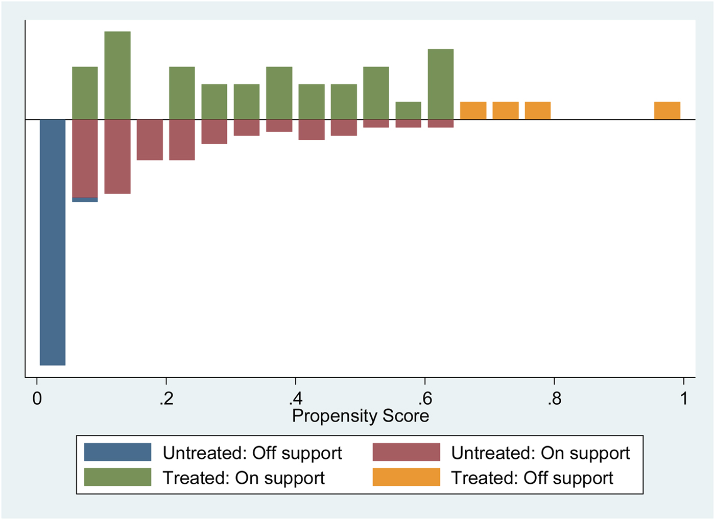
Figure 1. Histogram of Propensity Score by Treatment Status
The number of observations dropped from analysis is 61 non-participant towns with propensity score less than 0.05 and 4 participant towns with propensity score above 0.65. The inference of treatment effect cannot be generalized to the population and is reduced to the subset of 30 towns with MSW user fees. Although matching on common support results in fewer observations, an advantage is the remaining set of towns is similar in covariates which influence the decision to adopt MSW user fees and in MSW waste generation
Common support implies omitting all observations of participant towns’ propensity scores that are above the maximum propensity score for the non-participant towns, and omitting all observations for non-participant towns’ propensity scores that are below the minimum propensity score for the participant counties. Matching on a common support makes it evident whether or not comparable non-participant units are available for each participant unit. In the matching literature, the benefit of matching on common support is contrasted to regression analysis when observations of participants and non-participants are clustered into two distinct groups and effects are estimated “solely by projection into regions where there are no data points” (Smith Reference Smith2006).
Standard errors and 95 percent confidence intervals were estimated using bootstrapping with 1,000 replicates and are listed in Table 4. The ATET estimates are statistically significant at the 0.05 significance level. The use of bootstrapping to calculate the variance of kernel matching estimators is subject to debate given there is no theoretical justification for bootstrapping to estimate the variance of matching estimators. Some research suggests bootstrapping methods may not give correct results (Imbens Reference Imbens2004), so results derived using this method should be used with caution.
Estimates of average treatment effects (ATE) using ordinary least squares (OLS) with an indicator variable for policy adoption and the same set of explanatory variables used in the logit model and the estimated propensity score are listed in Table 4. Two estimates are listed. One is an ATE estimate of −801 pounds reduction per household using the full data set of 180 towns with 34 towns using MSW user fees. When OLS estimation is limited to the common support used for propensity score matching with 115 towns) the estimate of program impact is −748 pounds per household. Both estimates are statistically significant at a 0.01 significance level.
Table 4 also includes an estimate of the average treatment effect on the untreated (ATEUT). This is a measure of the expected average effect if towns who have not voluntarily adopted MSW user fees were required to adopt MSW user fees. The ATEUT is −649 pounds per household per year using nearest neighbor matching and −771 pounds per household per year using a kernel estimator with 0.06 bandwidth. Both estimates are less than the effect for towns who have voluntarily adopted MSW user fees.
The property for matching estimators to be asymptotically unbiased is premised on the conditional independence assumption (CIA). When matching is conditioned on a set of variables that influence the decision to implement MSW user fees and MSW waste generation, then the potential outcome variable is independent of treatment assignment.
This assumption also extends to variables which influence policy choice and waste generation that are not observed. For example, if households in communities with MSW user fees are also more motivated to reduce waste generation relative to households located in town without MSW user fees, then the above estimates of program effects may be partially attributed to the MSW user fee and the unobserved household motivation.
Sensitivity analysis is conducted to evaluate the robustness of empirical results to potential bias attributed to unobserved variables. By definition, because unobserved variables cannot be directly modeled, the approach to sensitivity analysis is to estimate the level of effect an unobserved variable would have to exert on the derived estimates such that the results are no longer statistically significant. If a relatively minor effect renders the results not statistically significant, then the estimates are not robust.
The results of a Rosenbaum and Rubin (2002) sensitivity analysis are listed in Table 6. The test statistic, Gamma (Γ), is calculated as a ratio of odds for two observations. Description and derivation of the Rosenbaum bounds are presented in Rubin (Reference Rubin2006), Guo and Fisher (Reference Guo and Fisher2010), and DiPrete and Gangl (Reference DiPrete and Gangl2004). Following Guo and Fisher (Reference Guo and Fisher2010), the odds ratio that two towns i and j adopt MSW user fees is:
 $$[{\rm \pi }_i/({\rm 1} - {\rm \pi }_i)]/[{\rm \pi }_j/({\rm 1} - {\rm \pi }_j)] = [{\rm \pi }_i({\rm 1} - {\rm \pi }_j)]/[{\rm \pi }_j({\rm 1} - {\rm \pi }_i)]$$
Table 6. Rosenbaum Bounds

If two towns have the same covariates x i = x j, then the probability of adopting MSW user fees is the same for each town πi = πj and the above odds ratio will equal 1. However, if an unobserved variable affects the probability of policy adoption and MSW generation, the two towns with similar covariates may have different probabilities of policy adoption, πi ≠ πj, and the above odds ratio will be different from 1. Rosenbaum (Reference Rosenbaum2002) derived a test statistic which can be used as a bound of the above odds ratio:
 $${\rm 1}/\Gamma \le [{\rm \pi }_i({\rm 1} - {\rm \pi }_j)]/[{\rm \pi }_j({\rm 1} - {\rm \pi }_i)]\; \le \Gamma $$
when Γ = 1, then πi = πj, so that the odds ratio is 1 assuming x i = x j . When Γ = 2 and assuming similar town covariates, the two towns could differ in probability of policy adoption by as much as a factor of 2, and one town may be twice as likely to adopt MSW user fees due to an unobserved variable. A Wilcoxon test statistic is calculated based upon the statistical significance in the outcome variable which corresponds for each level of Γ. Assuming the estimates are free of hidden bias, values of Γ close to 1 in which the corresponding p-value is at or above 0.05 indicate the results are sensitive to small changes induced by a hidden bias. High values of Γ are associated with robust results in which the effect of hidden bias must be relatively large to render the estimates not significant.
Based upon the results listed in Table 6 a Γ level of 3.75 has a p-value of 0.053. The interpretation is that the odds ratio would have to change by a factor of 3.75 to render the estimates statistically insignificant at a significance level of 0.05. Based upon the Rosenbaum bounds sensitivity analysis, the results listed in Table 4 from using the kernel estimator with a bandwidth of 0.06 are relatively robust and thus are less sensitive to potential bias from an omitted variable.
Included in Table 6 are estimates of the equivalent hidden bias associated with different Γ levels. To render the estimated treatment effect insignificant as a result of hidden bias is equivalent to increasing median housing values by $46,000 above the current mean value of $224,000 (20 percent increase) or increasing membership in a conservation organization from the current mean level of 1.4 members per 100 households to 3.6 members per 100 households (257 percent increase).
Concluding Remarks
This study uses a cross-sectional data set of 180 towns located in New Hampshire with 34 towns using a form of MSW user fees in the year 2008. The ATET ranges from an average annual reduction from 631 pounds per household to 823 pounds per household. This represents a reduction from 42 percent to 54 percent from an average MSW of 1,511 pounds per household for towns without MSW user fees. Based upon bootstrapping to estimate the estimator's standard error, the estimates are statistically significant at a significance level of 0.05.
The results were obtained from an empirical application of propensity score matching to estimate treatment effects of unit-based pricing on household solid waste disposal. Empirical advantages associated with matching estimation are the ability to derive estimators of treatment effects for towns that have implemented some form of unit-based pricing and also to estimate treatment effects for those town which have not adopted MSW user fees but may choose to do so in the future. Similar treatment effects cannot be estimated using linear regression.
Matching methods do not require a priori specification of functional form as required by linear regression models and are thus less restrictive. Given that the normalized difference for 5 of the 8 explanatory variables exceeds 0.25, linear regression estimates of average treatment effects may not be globally accurate (Imbens and Wooldridge Reference Imbens and Wooldridge2009). An advantage of matching methods is that there are fewer econometric assumptions regarding functional form compared to linear regression methods.
Furthermore, as noted earlier, given that matching is conducted within an interval of common support it avoids the occurrence of regression analysis when observations of participants and non-participants are clustered into two distinct groups and effects are estimated “solely by projection into regions where there are no data points” (Smith Reference Smith2006). The estimates of ATET and ATEUT using matching methods suggest the effects of MSW user fees are heterogeneous across towns. Linear regression assumes these two values are equal.
The choice of evaluation method is motivated by: (1) the type of policy question to be answered and (2) whether program response is assumed to be heterogeneous or homogeneous across units. Matching methods are used to evaluate the program effect on subsets of the population when effects are expected to vary across units (Blundell and Dias Reference Blundell and Dias2002).
For this study, the ATET is used to estimate the effect of MSW user fees on municipalities that use some form of MSW user fees. Because communities self-select to implement MSW user fees, the program effects are assumed to vary across municipalities.
The results of this study suggest that the effect of MSW user fees range from a 42 percent to 54 percent reduction in the level of household solid waste disposed of each year. Prior results from empirical studies using linear regression to estimate the program effect suggest a 27 percent to 41 percent reduction reported by Kinnaman and Fullerton (Reference Kinnaman and Fullerton2000), a 38 percent to 60 percent reduction reported by Dijkgraaf and Gradus (Reference Dijkgraaf and Gradus2009), and a 44 percent to 71 percent reduction reported by Huang, Halstead, and Saunders (Reference Huang, Halstead and Saunders2011). The higher values with Kinnaman and Fullerton (Reference Kinnaman and Fullerton2000) and Huang, Halstead, and Saunders (Reference Huang, Halstead and Saunders2011) results are associated with estimates after correcting for policy endogeneity.
Areas for further investigation include the effect of MSW user fees on recycling rates and the effect of MSW user fees over time. Although there is an increase in the level of recycling associated with communities using MSW user fees, cursory examination of recycling rates for communities with and without MSW user fees does not find the difference to be statistically significant at conventional levels. This warrants further investigation.
This analysis was conducted using cross-sectional data for the year 2008. Results are sensitive to the selected time period. Analysis conducted for prior years finds smaller impacts. The U.S. economy experienced a significant recession in 2008. Further consideration should be given to controlling for the potential effect of an economic downturn on household behavior of waste generation, though we argue based on empirical data that per-capita waste generation after and during the great recession did not differ markedly. MSW user fees may have a differential impact on household waste disposal behavior during economic recessions compared to economic expansions. Are households who pay a user fee for trash disposal relatively more responsive to MSW user fees during a recessionary period compared to periods of economic prosperity?
Some studies have suggested the observed decrease in MSW disposal, but the absence of a corresponding increase in recycling may be attributed to illegal waste disposal. When a community adopts MSW user fees, there is concern that households choosing to avoid the additional cost will resort to “illegal dumping,” such as disposing garbage at trash collection bins used by locations serviced by private waste haulers. To date there are no empirical results suggesting illegal dumping is a significant outcome associated with communities using MSW user fees. The results for this study are premised on the assumption that the estimated reduction in household waste disposal is not offset by an increase in illegal solid waste disposal.


 Open access