


1. Introduction
Stratified turbulence facilitates the upwelling of deep, dense waters in the abyssal polar oceans, thereby enabling the closure of the meriodional overturning circulation (Wunsch & Ferrari Reference Wunsch and Ferrari2004). It is thought that this turbulence, at least far from boundaries, predominantly arises during discrete mixing events caused by the breaking of internal gravity waves generated by the flow of tidal currents over rough bottom topography (MacKinnon et al. Reference MacKinnon2017). Attempts to model these wave-breaking processes frequently use the destabilisation of a parallel shear flow as the paradigm by which turbulence is generated, a physically plausible approach if we assume that the primary instabilities occur on a scale that is small compared with the internal waves. Kelvin–Helmholtz instability (KHI) is perhaps the most commonly studied shear instability, having been observed in a variety of oceanic environments, for example, above continental shelves (Moum et al. Reference Moum, Farmer, Smyth, Armi and Vagle2003) and in deep ocean trenches (van Haren et al. Reference van Haren, Gostiaux, Morozov and Tarakanov2014). The way in which flows that exhibit KHI become turbulent and the properties of the subsequent mixing has been the subject of multiple recent studies that invoke high-resolution direct numerical simulations (DNS) at increasingly large Reynolds number  ${Re}$ and Prandtl number
  ${Pr}$ (e.g. Mashayek & Peltier Reference Mashayek and Peltier2012a,Reference Mashayek and Peltierb; Salehipour, Peltier & Mashayek Reference Salehipour, Peltier and Mashayek2015).
The magnitude of the (essentially vertical) density flux across isopycnals associated with a turbulent mixing event depends on the percentage of kinetic energy available to turbulence which irreversibly contributes to this flux, a quantity commonly referred to as the mixing efficiency  $\eta$ which will be formally defined in § 3, though as noted by Gregg et al. (Reference Gregg, D'Asoro, Riley and Kunze2018), great care must be taken to understand the precise definition being used, especially when comparing the results of different studies. An appropriately defined mixing efficiency may be used to compute a diapycnal eddy diffusivity
  $K_\rho$ from measurements of dissipation
  $\varepsilon$ and buoyancy frequency
  $N$ in the ocean via an equation of the form
 \begin{equation} K_\rho = \varGamma \varepsilon/ N^2, \end{equation}
where the flux coefficient  $\varGamma \equiv \eta /(1-\eta )$ is often assumed to take the constant value
  $0.2$ corresponding to the upper bound originally proposed by Osborn (Reference Osborn1980), in broad alignment with ocean measurements obtained via tracer release experiments (Gregg et al. Reference Gregg, D'Asoro, Riley and Kunze2018). There is, however, considerable evidence to suggest that much larger values of
  $\varGamma$ are accessible in some turbulent regimes, particularly in flows that exhibit significant overturnings in the density field, as might be expected to be associated with the breakdown of KHI.
Recent DNS studies of stratified shear turbulence have demonstrated that mixing efficiency, and hence also  $\varGamma$, appear to depend on time-evolving non-dimensional parameters such as the buoyancy Reynolds number
  ${Re}_b = \varepsilon /\nu N^2$ and the gradient Richardson number
  ${Ri}_g = N^2/S^2$ (e.g. Salehipour & Peltier Reference Salehipour and Peltier2015), where
  $\nu$ is the kinematic viscosity and
  $S$ is some appropriate measure of the vertical shear. Such dependencies have been used to develop multi-parameter schemes for calculating mixing efficiency in the ocean (Salehipour et al. Reference Salehipour, Peltier, Whalen and MacKinnon2016b). An alternative, though inevitably related approach, is to assume that measures of mixing such as the flux coefficient can be parameterized in terms of appropriate characteristic length scales in the flow (Ijichi & Hibiya Reference Ijichi and Hibiya2018; Garanaik & Venayagamoorthy Reference Garanaik and Venayagamoorthy2019), typically related to underlying properties of the turbulence. Of particular relevance is the Thorpe scale
  $L_T$, a purely geometrical construct describing the extent of overturning motions in the density field. The ratio
  $R_{OT}=L_O/L_T$ of this scale to the Ozmidov scale
  $L_{O} = (\varepsilon /N^3)^{1/2}$, which quantifies the upper bound on turbulent vertical scales that may be assumed to be largely unaffected by ambient stratification, is often used to diagnose mixing from oceanographic measurements in a method that relies on assuming that
  $R_{OT} = O(1)$ (see e.g. Waterhouse et al. Reference Waterhouse2014). For flows that have significant overturnings such as turbulence produced by KHI, it has been shown that we can have
  $L_T \gg L_O$, particularly early in the life cycle when the turbulence is relatively ‘young’, leading to the possibility of considerably underestimating mixing in ocean flows (Chalamalla & Sarkar Reference Chalamalla and Sarkar2015; Mater et al. Reference Mater, Venayagamoorthy, Laurent and Moum2015; Scotti Reference Scotti2015; Mashayek, Caulfield & Peltier Reference Mashayek, Caulfield and Peltier2017; Mashayek, Caulfield & Alford Reference Mashayek, Caulfield and Alford2021).
There has been recent interest in the applicability of scaling laws for the flux coefficient  $\varGamma$ which generally take the form
  $\varGamma \sim R_{OT}^{-r}$, where the value of the exponent
  $r$ depends on the extent by which turbulent motions are suppressed by the stratification. Closely related to the Thorpe scale is the Ellison scale
  $L_E$, which measures the turbulent fluctuations in the density field compared with the background stratification. Whilst observational measurements of
  $L_E$ are more difficult to obtain than the Thorpe scale
  $L_T$ due to the need for time-series data rather than a single vertical profile (Cimatoribus, van Haren & Gostiaux Reference Cimatoribus, van Haren and Gostiaux2014),
  $L_E$ is an appealing alternative because it explicitly characterises the relationship between the turbulence and stratification in the flow (Ivey, Bluteau & Jones Reference Ivey, Bluteau and Jones2018).
As argued by Ivey et al. (Reference Ivey, Bluteau and Jones2018), however, it is always important to remember that the key quantity of practical interest is the diapycnal eddy diffusivity  $K_\rho$, and
  $\varGamma$ is an intermediate parameter arising from the modelling presented by Osborn (Reference Osborn1980) defined using various terms in the evolution equation for turbulent kinetic energy. Instead, using a method originally proposed by Osborn & Cox (Reference Osborn and Cox1972), it is perhaps more natural to parameterize the eddy diffusivity in terms of an appropriate definition of the density variance destruction rate
  $\chi$ via the equation
 \begin{equation} K_\rho = \chi/N^2, \end{equation}
as this directly relates mixing of density (and destruction of available potential energy) to the eddy diffusivity, without appealing to possibly uncorrelated properties of the turbulent kinetic energy budget (Caulfield Reference Caulfield2021). Indeed,  $\chi$ is often used as a diagnostic for local mixing. That the two are inextricably linked becomes obvious if we note that we can recover (1.2) from (1.1) by simply choosing to define mixing efficiency
  $\eta$ from the outset as
  $\eta = \chi /(\chi +\epsilon )$ in the definition of the flux coefficient
  $\varGamma$.
Even once a mixing parameterization has been selected, additional complications arise. Firstly, any approach based on quantities that can be defined locally as well as globally raises questions about the averaging involved to determine the various parameters, due to the inherent spatio-temporal variability and anisotropy of stratified turbulent flows (see, for example, Arthur et al. Reference Arthur, Venayagamoorthy, Koseff and Fringer2017). Secondly, and for KHI-induced turbulence in particular, ‘history matters’ greatly in the sense that varying initial conditions and early flow behaviour can leave an imprint on the subsequent mixing, not least through the lasting influence of the primary billow overturning. Highly anisotropic secondary instabilities that occur on that billow during its breakdown to turbulence can lead to very efficient, indeed ‘optimal’ mixing (Mashayek & Peltier Reference Mashayek and Peltier2013; Mashayek et al. Reference Mashayek, Caulfield and Peltier2017, Reference Mashayek, Caulfield and Alford2021), with the development of such structures depending on the initial state of the flow (Mashayek, Caulfield & Peltier Reference Mashayek, Caulfield and Peltier2013).
Whether fully formed billows that support these instabilities occur at all for more realistic initial flow conditions is also not known. In a study with significant implications for mixing in real-world environments, Kaminski & Smyth (Reference Kaminski and Smyth2019) show that mixing efficiency may be significantly reduced for KHI-induced breakdown in a field of background noise designed to represent vestigial turbulence from a previous mixing event. They demonstrate convincingly that this reduction is due to the fact that the growing primary billow is disrupted by turbulence before it can fully develop, a feature also observed in a similar study by Brucker & Sarkar (Reference Brucker and Sarkar2007). Even in a simple KHI set-up, there are clearly a large number of variables and flow modifications that can affect the dynamics and in particular the mixing, and it is natural to ask whether such a set-up is at all useful for describing ocean processes which are in general much more complex than their idealised model counterparts.
Motivated by this fundamental question, here we will focus on the influence of a far field stratification on the turbulent dynamics and mixing produced by KHI in a shear layer. In a manner similar to the recent work of VanDine, Pham & Sarkar (Reference VanDine, Pham and Sarkar2021), we aim to determine the effects of a constant linear background stratification on the turbulent mixing produced by KHI in a shear layer by comparison with a classical two-layer set-up that has background density and velocity profiles given by a hyperbolic tangent function, quantifying our results both in terms of an appropriately defined mixing efficiency as well as in terms of the eddy diffusivity. In particular, we investigate the use of the density variance destruction rate  $\chi$ as a diagnostic for local mixing, using our results to comment on the action of secondary instabilities in producing ‘optimal’ mixing. We explore how measures of mixing vary with local values of
  ${Re}_b$ and
  ${Ri}_g$, as well as appropriately defined characteristic length scales in the flow, using our results to argue which aspects of mixing by KHI can be said to be generic in the sense that they are not largely influenced by the presence of a far field stratification. We use our comparison of mixing properties in different background stratifications to investigate two specific important parameterization issues. Firstly, we investigate the applicability of a number of recently proposed scaling laws for the flux coefficient
  $\varGamma$ in terms of characteristic length scales to turbulence produced by KHI. In particular, we are interested in whether or not the Ellison scale
  $L_E$ is a more appropriate density length scale in this context than the Thorpe scale
  $L_T$. Secondly, we investigate different parameterizations of the eddy diffusivity using appropriate definitions of either the flux coefficient
  $\varGamma$ or the buoyancy variance destruction rate
  $\chi$. The remainder of this paper is organised as follows. In § 2 we describe the two different background density profiles used in our comparison and the set-up for the DNS performed. The results of the simulations are presented in § 3, where we use a variety of global and local quantitative measures of mixing to investigate how the evolution of KHI depends on the background stratification, and test various proposed parameterizations. Finally, we discuss the importance of our results for the quantification of ocean mixing produced by KHI in § 4.
2. Simulations
2.1. Theory
A classical KHI set-up, widely studied using numerical simulations, has background velocity and density profiles given by a hyperbolic tangent function of depth. Denoting dimensional variables with a star, we have
 \begin{equation} \overline{u}^*(z^*) = {\rm \Delta} u^*\tanh\left(\frac{z^*}{h^*}\right),\quad \overline{\rho}^*(z^*) = \rho_a^* -{\rm \Delta} \rho^* \tanh\left(\frac{z^*}{h^*}\right). \end{equation}
Here  $h^*$ is half of the shear layer thickness,
  ${\rm \Delta} u^*$ and
  ${\rm \Delta} \rho ^*$ are half of the velocity and density differences across the shear layer, respectively, and
  $\rho _a^*\gg {\rm \Delta} \rho ^*$ is a reference density. Historically, these profiles have been widely studied in the context of shear instability because they give rise to analytical solutions of the Taylor–Goldstein equation for inviscid stratified shear flow (Holmboe Reference Holmboe1962). More generally, they are similar to those realised in laboratory experiments (see Thorpe (Reference Thorpe2005) for an overview). We will compare the evolution of the flow described above to flows with a linear background density profile, i.e.
 \begin{equation} \bar{u}^*(z^*) = {\rm \Delta} u^*\tanh\left(\frac{z^*}{h^*}\right),\quad \bar{\rho}^*(z^*) = \rho_a^* -{\rm \Delta} \rho^* \left(\frac{z^*}{h^*}\right). \end{equation}
Such conditions are known to produce a distinctive layer-interface structure via the destruction of KHI, with the far field stratification enabling internal gravity waves to propagate energy away from the shear layer (Fritts et al. Reference Fritts, Bizon, Werne and Meyer2003; Pham, Sarkar & Brucker Reference Pham, Sarkar and Brucker2009; Watanabe et al. Reference Watanabe, Riley, Nagata, Onishi and Matsuda2018; VanDine et al. Reference VanDine, Pham and Sarkar2021). We class the set-ups (2.1a,b) and (2.2a,b) as T (for ‘tanh’) and L (for ‘linear’), respectively.
Flow dynamics is governed by the Navier–Stokes equations with a Boussinesq approximation in the form
 $$\begin{gather} \frac{{\rm D}u_i}{{\rm D}t} ={-} \frac{\partial p}{\partial x_i} - {Ri}_0\rho \delta_{i3} + \frac{1}{Re}\frac{\partial ^2 u_i}{\partial x_j^2}, \end{gather}$$
 $$\begin{gather}\frac{\partial u_i}{\partial x_i} = 0, \end{gather}$$
 $$\begin{gather}\frac{{\rm D} \rho}{{\rm D} t} = \frac{1}{{Re} {Pr}} \frac{\partial^2\rho}{\partial x_i^2}, \end{gather}$$
in which repeated indices represent summation and  $i,j\in \{1,2,3\}$. Non-dimensional variables are defined by
 \begin{equation}
t = t^* \Delta u^*/h^*,\quad x_i = x_i^*/h^*, \quad u_i = u_i^*/\Delta u^*, \quad\rho = \rho^*/\Delta \rho^*,\quad p = p^* /(\rho_a^*\Delta u^{*2}),
\end{equation}
\begin{equation}
t = t^* \Delta u^*/h^*,\quad x_i = x_i^*/h^*, \quad u_i = u_i^*/\Delta u^*, \quad\rho = \rho^*/\Delta \rho^*,\quad p = p^* /(\rho_a^*\Delta u^{*2}),
\end{equation}
where  $p^*$ and
  $\rho ^*$ are departures from hydrostatic balance. We assume a linear equation of state relating density and temperature, neglecting salinity so that double-diffusive effects do not apply.
The evolution of the flow is characterised by three dimensionless parameters, namely the (bulk) Richardson, Reynolds and Prandtl numbers defined respectively by
 \begin{equation} {Ri}_0 = \frac{g^*h^*{\rm \Delta} \rho^* }{\rho_a^* {\rm \Delta} u^{*2}},\quad {Re} = \frac{h^*{\rm \Delta} u^*}{\nu^*},\quad {Pr} = \frac{\nu^*}{\kappa^*}, \end{equation}
where  $g^*$ is the acceleration due to gravity, and
  $\nu ^*$ and
  $\kappa ^*$ are the respective momentum and density diffusivities. Note that the Richardson number
  ${Ri}_0$ corresponds to the minimum initial value of the gradient Richardson number
 \begin{equation} {Ri}_g \equiv \frac{N^2}{S^2} = \frac{-Ri_0\text{d} \bar{\rho}/\text{d} z}{(\text{d} \bar{u}/\text{d} z)^2}, \end{equation}
which occurs at the centre of the shear layer  $z=0$ for both T and L flows.
2.2. Simulation set-up
We use the pseudo-spectral time-stepping code Diablo (Taylor Reference Taylor2008) to solve (2.3)–(2.5) in a channel geometry which is periodic in the horizontal ( $x$ and
  $y$) directions. The vertical extent is set to be
  $L_z=30$ to minimise boundary effects, with the numerical grid taken to be more finely spaced in the region
  $-5\leq z \leq 5$, comfortably fitting the extent of the growing billow and subsequent turbulent region for all simulations presented. Outside of this region, the cell height is gradually stretched by approximately
  $25\,\%$ every 10 cells. For class T simulations, we impose free-slip, no-flux boundary conditions at the top and bottom of the domain, whilst for class L simulations, we have a thin sponge layer in the regions
  $-15\leq z \leq -12.5$ and
  $12.5\leq z\leq 15$ to absorb incoming internal waves. A Reynolds number of
  ${Re}=6000$ is expected to be sufficiently high to ensure the emergence of the ‘zoo’ of secondary instabilities described in Mashayek & Peltier (Reference Mashayek and Peltier2012a,Reference Mashayek and Peltierb), as well as suppressing the phenomenon of vortex pairing (Mashayek & Peltier Reference Mashayek and Peltier2013).
Therefore, we focus on the breakdown of a single KHI billow and take the streamwise extent of the domain to be one wavelength of the fastest growing normal mode (FGM) of the linear theory calculated using a matrix code by Smyth, Moum & Nash (Reference Smyth, Moum and Nash2011). The spanwise extent of the domain is  $L_y=4$ for all simulations. Based on the work of Mashayek et al. (Reference Mashayek, Caulfield and Peltier2013) who use a similar set of initial values of
  ${Ri}_0$ at
  ${Re}=6000$ and note that the flow dynamics is unchanged upon doubling the spanwise extent, this is expected to be sufficiently large to accommodate the significant modes of secondary instability emerging from the primary billow. Wider extents can accommodate a range of spanwise interactions between adjacent KHI billows that we do not consider here (Fritts et al. Reference Fritts, Wieland, Lund, Thorpe and Hecht2021). For class L simulations, we choose
  ${Ri}_0$ with the aim of producing a mixing layer with comparable height to each class T simulation, as we demonstrate below. We also set the Prandtl number to a nominal value of
  $Pr =1$. Table 1 displays the class, initial parameter values and domain size for each simulation performed. The grid resolution is chosen to resolve scales down to
  $2.5$ times the Kolmogorov length scale
  $L_K$ defined by
  $L_K = \min _{z} ((1/{Re})^3 /\bar {\varepsilon }(z,t))^{1/4},$ where an overline denotes averaging over horizontal planes.
Table 1. Class, flow parameters and grid sizes for each DNS, as well as the time  $t_{2\text{-}D}$ taken to reach maximal billow amplitude in two-dimensional (2-D) roll-up simulations. All simulations shown have
  ${Re}=6000$,
  ${Pr}=1$, with
  $L_y=4$ and
  $L_z=30$. Here
  $N_x$,
  $N_y$ and
  $N_z$ are the number of grid points in the streamwise, spanwise and vertical directions, respectively, whilst
  $N_z^c$ is the number of vertical grid points in the central region
  $-5\leq z \leq 5$.

To initialise the flow in a way that allows for a consistent comparison of the breakdown to turbulence between simulations, particularly with regards to the emergence of secondary instabilities, we have chosen to perturb all simulations again at the point of maximal billow amplitude with an additional small uniform noise perturbation imposed on the density and velocity fields. A brief investigation detailed in the Appendix reveals that the emergence of secondary instabilities on the primary KHI billow in freely evolving simulations is highly sensitive to the grid resolution in the streamwise and vertical directions, with some of these instabilities being ‘unphysically’ perturbed at an early time by noise arising from numerical truncation errors at the grid scale. Whilst this is a subtle point, in order to be completely consistent in our comparison and to avoid results that may depend on grid resolution, we would argue that it is most convenient to perform a two-dimensional (2-D) simulation of the roll-up of the primary KHI billow up to the point of maximal billow amplitude before uniformly projecting the resulting flow state onto the spanwise direction in three-dimensional (3-D) space and adding a further noise perturbation to initiate the 2-D and 3-D secondary instabilities in a largely unbiased manner, at the same relative time across all simulations. The additional perturbation takes the form of uniform white noise of amplitude  $10^{-3}$ added to the velocity and density fields.
The time  $t_{{2\text{-}D}}$ of maximal billow amplitude in the 2-D roll-up simulations is defined at the maximum value of the inherently 2-D component of the kinetic energy
  $\mathcal {K}_{2\text{-}D} = (u_{2\text{-}D}^2 + v_{2\text{-}D}^2 + w_{2\text{-}D}^2)/2$, where the inherently 2-D components of the velocity field
  $(u_{2\text{-}D}, v_{2\text{-}D}, w_{2\text{-}D})$ are defined via a 3-D Reynolds decomposition of the flow as in Caulfield & Peltier (Reference Caulfield and Peltier2000). The roll-up simulations are initialised with a perturbation in the form of the FGM from the linear theory to facilitate fast primary billow growth. Importantly, each of these simulations is run at a resolution high enough such that secondary instabilities are not significantly evolved at the point of maximum billow amplitude (i.e. any numerical noise present will be small compared with the subsequent additional perturbation). We are implicitly assuming that the growth of the primary billow is inherently 2-D, a feature that is consistent with the recent studies of Mashayek & Peltier (Reference Mashayek and Peltier2013) and Salehipour et al. (Reference Salehipour, Peltier and Mashayek2015). For completeness, the reference values of
  $t_{2\text{-}D}$ from the roll-up simulations are included in table 1; these correspond to the start time
  $t=0$ in fully 3-D simulations. Whilst this choice of set-up is obviously highly specific, we will see that these small modifications to the classical idealised KHI billow evolving from a background shear flow can produce quite distinctive differences in the subsequent dynamics, highlighting the difficulties in using any single idealized DNS model to infer general ocean mixing properties.
3. Results
3.1. Evolution of the turbulent mixing layer
For all of the simulations listed in table 1, we take non-dimensional time  $t=0$ to correspond to the time of billow saturation, or maximal
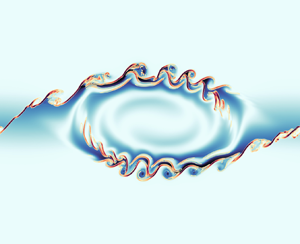
  $\mathcal {K}_{2\text{-}D}$, as described above. To get an overview of flow behaviour, figure 1 shows successive 2-D contour plots through
  $y=0$ of the spanwise vorticity field
  $\omega _y =\partial _z u - \partial _x w$, demonstrating the turbulent transition behaviour for flows L10 and T16. The presence of the ambient stratification in the L10 flow means that a considerably lower
  ${Ri}_0=0.10$ produces a billow of similar height to its T16 counterpart with
  ${Ri}_0=0.16$. As is to be expected at
  ${Re}=6000$ following the investigations of Mashayek & Peltier (Reference Mashayek and Peltier2012a,Reference Mashayek and Peltierb), the noise perturbation at
  $t=0$ triggers a variety of rapidly emerging secondary instabilities that facilitate the breakdown to turbulence, which then becomes increasingly isotropic within the mixing layer as it evolves. Analogous behaviour is observed for the simulations L13 and T19. The main qualitative difference between the class L and T simulations is the presence of faint internal gravity waves in the L simulations that propagate away from the turbulent layer in class L simulations through the turbulent/non-turbulent layer interface (TNTI), which is visible most distinctly at the turbulent layer boundary in figure 1(d). (The dynamics of the TNTI are discussed in detail in Watanabe et al. Reference Watanabe, Riley, Nagata, Onishi and Matsuda2018.) We note here that the relatively weak far field stratification in both L simulations means that the total energy propagated away from the shear layer by gravity waves during the mixing process is small compared with the initial kinetic energy (
 ${<}1\,\%$) and far field turbulent fluctuations are insignificant in magnitude compared to within the turbulent region, at least whilst more intense turbulence persists. This is the period during which the majority of irreversible mixing takes place; hence, for the present study, we will not be largely concerned with internal wave effects and will instead focus primarily on the dynamics within the turbulent layer. Stronger far field stratifications may result in larger amounts of energy extraction from the turbulent region. For example, Pham et al. (Reference Pham, Sarkar and Brucker2009) show that when the shear layer lies above a region of stronger stratification with
  $N^2 = -{Ri}_0\partial \bar {\rho }/\partial z \geq 0.25$, the amount of turbulent energy transported into the far field by internal waves can be up to 15 % of the initial mean kinetic energy inside the shear layer. Such a set-up might be more appropriate to model, for example, a turbulent shear layer in the ocean thermocline, as opposed to more weakly stratified abyssal waters.

Figure 1. Spanwise slices through  $y=0$ for various indicated times during the turbulent transition phase of flow showing contours of spanwise vorticity for simulations (a–d) L10 and (e–h) T16.
To investigate further the similarities and differences between the mixing layers produced by KHI in the L and T simulations, we examine the evolution of the horizontally averaged turbulent dissipation  $\bar {\varepsilon '}(z,t) \equiv \overline {\partial _j u'_i\partial _j u'_i}/{Re}$, the normalized buoyancy frequency
  $N^2(z,t)/{Ri}_0 = -\partial \bar {\rho }/\partial z$ and the local gradient Richardson number
  ${Ri}_g(z,t)$ defined in (2.8). The results are shown in figure 2, where we also plot the evolution of the height of the turbulent mixing layer as measured in two different ways. Firstly, we plot the momentum thickness
 \begin{equation} \ell_u(t) = \int_{{-}L_z/2}^{L_z/2} (1-\bar{u}(z,t)^2)\,\textrm{d} z \end{equation}
defined by Smyth & Moum (Reference Smyth and Moum2000) as an estimate for the vertical extent of the mixing layer for simulations that have a background shear profile given by a hyperbolic tangent function (note their definition includes an additional factor of 4 due to differences in the non-dimensionalization). Secondly, similar to VanDine et al. (Reference VanDine, Pham and Sarkar2021), we identify a so-called ‘transition layer’ (TL) as a region of enhanced stratification (specifically, we demarcate the edges of these regions where  $|\partial \bar {\rho }/\partial z|$ becomes larger than the far field stratification by more than 10 % of its maximum value) immediately above and below the mixing layer and plot the evolution of the outer boundaries of these layers for each simulation.

Figure 2. Time-evolving vertical profiles of (a–d) horizontally averaged turbulent dissipation  $\bar {\varepsilon '} (z,t)$, (e–h) normalized buoyancy frequency
  $N^2(z,t)/Ri_0$ and (i–l) gradient Richardson number
  $Ri_g(z,t)$ for each simulation as indicated in the top right-hand corner of the panels. Dashed lines are the contours
  $z=\pm \ell _u(t)/2$, whilst dot–dashed lines are the contours marking the edges of the transition layers.
Looking at the structural evolution of  $\bar {\varepsilon '}$, flows T16 and L10 are qualitatively very similar in terms of the extent of the turbulent mixing layer, the patterns of more intense turbulence within the mixing layer and the time taken for turbulence to decay. Flows T19 and L13 are likewise qualitatively similar. There are slight differences in
  $\bar {\varepsilon '}$ between L and T simulations during the early part of the flow, with the asymmetry of young turbulence rotating around the distorted laminar billow core (as seen in figure 1c) causing wave-like patterns at the edge of the mixing region in L simulations for
  $t<40$. More obvious differences between L and T simulations are visible in the evolution of the background stratification
  $N^2/Ri_0$, which is much larger in the TLs for L simulations than it is for T simulations. The importance of the TL has been investigated in detail by VanDine et al. (Reference VanDine, Pham and Sarkar2021), who argue that the dynamics within this region are important and should be included when computing bulk flow statistics. We will explore this issue further in § 3.2. Finally, looking at the evolution of the local gradient Richardson number
  ${Ri}_g$, we see that the turbulent breakdown in both L and T simulations is characterised by small local values of
  ${Ri}_g$ in the centre of the mixing layer. Once the turbulence starts to decay, however, class L flows exhibit a distinct increased frequency of relatively larger values of
  ${Ri}_g$ between the TLs, despite the fact that the dissipation decays in an apparently similar manner between T and L simulations. We will discuss the importance of
  ${Ri}_g$ for parameterizing mixing in § 3.4.
In general, the observed similarities between corresponding L and T simulations are supported by the behaviour of  $\ell _u(t)$ and the boundaries of the TLs, which are both reasonable measures of the height of the mixing layer when turbulence is present. Based on the qualitative similarities between these two pairs of flows that have a similar mixing layer height, it is natural to ask whether the mixing taking place is also quantitatively similar, and whether the behaviour is generic enough such that attempts to parameterize its efficiency do not largely depend on the background stratification.
3.2. Local and global measures of mixing
In order to define mixing appropriately as an irreversible diffusive flux across isopycnals, it is important to distinguish between diabatic processes (those in which the physical properties of individual fluid parcels are modified) associated with mixing and adiabatic processes (those which modify only the distribution of parcels) associated with stirring in the flow. Proceeding as in Caulfield & Peltier (Reference Caulfield and Peltier2000), we divide the total potential energy  $\mathscr {P} = {Ri}_0 \langle \rho z \rangle$ into two parts, the background potential energy (BPE)
  $\mathscr {P}_B$ defined as
 \begin{equation} \mathscr{P}_B = {Ri}_0 \langle z \rho_B(z) \rangle, \end{equation}
and the available potential energy (APE)  $\mathscr {P}_A$ defined in the equation
 \begin{equation} \mathscr{P} = \mathscr{P}_B + \mathscr{P}_A. \end{equation}
The background density profile  $\rho _B(z)$ is obtained by adiabatically rearranging the density field into a gravitationally stable monotonic configuration. An important result obtained by Winters et al. (Reference Winters, Lombard, Riley and D'Asoro1995) states that, for an initially statically stable closed system, the potential energy of this configuration (i.e. the BPE) necessarily increases monotonically with time at a rate bounded below by the rate of diffusion of the mean laminar flow
  $\mathscr {D}_p = \int _{-L_z/2}^{L_z/2} z(\partial ^2\bar {\rho }/\partial z^2)\,\textrm {d} z$. Thus, by taking the time derivative of (3.3) we can write
 \begin{equation} \frac{{\rm d}\mathscr{P}_B}{{\rm d}t} = \mathscr{M} + \mathscr{D}_p,\quad \frac{{\rm d}\mathscr{P}_A}{{\rm d}t} ={-}\mathscr{B} - \mathscr{M}, \end{equation}
where  $\mathscr {B}\equiv -{Ri}_0 \langle \rho w \rangle$ is the volume integrated buoyancy flux and
  $\mathscr {M}$ is the strictly non-negative mixing rate that occurs due to macroscopic fluid motions. Note that we have
  $\mathscr {D}_p = 2{Ri}_0/({Re}{Pr} L_z)$ for T simulations and
  $\mathscr {D}_p=0$ for L simulations. From this definition of mixing, it is clear that BPE effectively increases ultimately due to conversion of energy from the APE reservoir. We compute
  $\mathscr {M}$ by taking a numerical time derivative of
  $\mathscr {P}_B$, which is evaluated at each time step using an approximation for
  $\rho _B(z)$ calculated using the probability density function of the full 3-D density field as described in Tseng & Ferziger (Reference Tseng and Ferziger2001).
The mixing rate  $\mathscr {M}$ is global by construction, and relies on the assumption that there is no flux of energy into or out of the domain. Whilst appropriate for our class T simulations in which energy is confined to the mixing layer by the lack of ambient stratification, possible issues arise in class L simulations where internal waves generated by turbulence cause fluctuations in the mixing rate
  $\mathscr {M}$ which become significant at later times when the turbulence is decaying. In order to isolate the mixing due to turbulence, it is more appropriate to invoke an alternative definition of mixing that can be applied to local regions. We appeal to a local definition of APE originally formulated by Holliday & Mcintyre (Reference Holliday and Mcintyre1981) and Andrews (Reference Andrews1981), which has seen recent interest applied to numerical simulations of turbulence in domains where boundary fluxes and large-scale internal waves complicate global definitions of mixing (Howland, Taylor & Caulfield Reference Howland, Taylor and Caulfield2021). Following Scotti & White (Reference Scotti and White2014), we define local APE density
  $E_{APE}$ as
 \begin{equation} E_{APE}(x,y,z,t)\equiv {Ri}_0 \int_{\rho_B(z,t)}^{\rho(x,y,z,t)} z-z_B(s,t)\,\textrm{d} s, \end{equation}
where  $z_B(\rho , t)$ is the reference height of the background density profile
  $\rho _B$ defined above, such that
  $z_B(\rho _B(z,t),t) = z$. This is equivalent to the work done in bringing a fluid parcel from its position in the sorted density profile to its actual position in the density field. Volume averaging the above, we recover the global definition
  $\mathscr {P}_A = {Ri}_0 \langle \rho (z-z_B) \rangle$, which may also be obtained from (3.2) and (3.3). To make progress in defining a local rate of mixing – that is, the rate of conversion from APE into BPE – first note that if we decompose the density field into the background profile
  $\rho _B$ plus a small perturbation
  $\delta \rho$, then to leading order we have
  $E_{APE}\sim {Ri}_0(\partial \rho _B/\partial z)^{-1} \delta \rho ^2/2$. If we assume that this decomposition is approximately equivalent to the turbulent flow decomposition achieved by horizontally averaging, i.e.
 \begin{equation} \rho(x,y,z,t) = \rho_B(z,t) + \delta\rho(x,y,z,t) \approx \bar{\rho}(z,t)+\rho'(x,y,z,t), \end{equation}
and make the additional strong assumption that the turbulent fluctuations are in fact small perturbations from a uniform imposed buoyancy gradient, then integrating over the turbulent region we obtain the following approximate expression  $\tilde {\mathscr {P}}_A$ for APE:
 \begin{equation} \tilde{\mathscr{P}}_A \equiv \frac{{Ri}_0}{2} \frac{\langle \rho'^2\rangle_T}{\langle \partial \bar{\rho}/\partial z \rangle_T }. \end{equation}
Here the angle brackets  $\langle \cdot \rangle _T$ denote a volume average taken over the extent of the mixing layer. The right-hand side can be recognised as an (appropriately scaled) definition of the variance of the density (or, equivalently, the buoyancy) relative to the horizontally averaged density (or buoyancy) distribution.
Assuming the denominator varies slowly in time compared with the numerator, the time evolution of (the approximation)  $\tilde {\mathscr {P}}_A$ is given by
 \begin{equation} \frac{{\rm d}\tilde{\mathscr{P}}_A}{{\rm d}t} = {Ri}_0\langle \rho' w'\rangle_T - \chi,\quad \chi\equiv\frac{{Ri}_0}{{Re} {Pr}} \frac{\langle \partial_i\rho'\partial_i\rho' \rangle_T}{\langle \partial \bar{\rho}/\partial z \rangle_T}, \end{equation}
where  $\chi$ is the appropriately normalised positive definite rate of density variance dissipation, often used as an alternative definition for mixing. One advantage of (3.8a,b) is that the numerator and denominator of
  $\chi$ can be defined pointwise, thus giving rise to a local definition of mixing. There is some degree of ambiguity as to how such pointwise measures should be interpreted. Based on the decomposition in (3.6), we consider two natural local interpretations of (3.8a,b), given by
 $$\begin{gather} \chi_{{loc}}(x,y,z,t) \equiv \frac{{Ri}_0}{{Re} {Pr}} \frac{{\partial_i\rho'\partial_i\rho'}}{ \langle \partial \bar{\rho}/\partial z \rangle_T}, \end{gather}$$
 $$\begin{gather}\tilde{\chi}_{{loc}}(x,y,z,t) \equiv \frac{{Ri}_0}{{Re} {Pr}}\frac{{\partial_i\rho'\partial_i\rho'}}{ \partial \widetilde{\bar{\rho}}/\partial z }, \end{gather}$$
where  $\widetilde {\bar {\rho }}(z,t)$ represents the horizontally averaged density field which has been sorted to be statically stable to avoid negative local gradients. The horizontal average
  $\overline {\tilde {\chi }_{{loc}}}$ is analogous to the alternative definition of local mixing used by Arthur et al. (Reference Arthur, Venayagamoorthy, Koseff and Fringer2017), who average in the spanwise direction only in their turbulent decomposition, as opposed to both horizontal directions. Note that the denominator in (3.10) is defined locally as a function of
  $z$ and
  $t$ whereas the denominator in (3.9) is a bulk average. In what follows we will be interested in whether the definitions (3.9)–(3.10) lead to accurate approximations of the globally evaluated irreversible mixing rate
  $\mathscr {M}$ when averaged over the turbulent layer. We have by definition that
  $\langle \chi _{{loc}} \rangle _T=\chi$, where
  $\chi$ is defined in (3.8a,b), and we correspondingly define the volume average
 \begin{equation} \tilde{\chi} \equiv \langle \tilde{\chi}_{{loc}}\rangle_T. \end{equation}
Howland et al. (Reference Howland, Taylor and Caulfield2021) find that  $\chi$, as defined in (3.8a,b), is a reasonable approximation for the mixing rate
  $\mathscr {M}$ in a variety of forced and unforced turbulent flows with an imposed uniform stratification, though their simulations display much weaker overturning behaviour than the KHI billows we consider here. Using simulations of breaking internal waves on slopes, Arthur et al. (Reference Arthur, Venayagamoorthy, Koseff and Fringer2017) show that the way in which local mixing rates are computed (in terms of how local density gradients are inferred from the denominator in
  $\chi$) can significantly modify values of the corresponding mixing efficiency. To compare the mixing rates
  $\mathscr {M}$,
  $\chi$ and
  $\tilde {\chi }$, we define three corresponding ‘instantaneous’ mixing efficiencies (i.e. based on mixing rates),
 \begin{equation} \eta_{\mathscr{M}}(t) \equiv \frac{\mathscr{M}}{\mathscr{M}+\langle \varepsilon \rangle},\quad \eta_{\chi}(t) \equiv \frac{\chi}{\chi+\langle \varepsilon \rangle_T},\quad \eta_{\tilde{\chi}}(t) \equiv \frac{\tilde{\chi}}{\tilde{\chi}+\langle \varepsilon \rangle_T}, \end{equation}
where we note that  $\varepsilon (x,y,z,t) = \partial _j u_i \partial _j u_i /{Re}$ is the total kinetic energy dissipation, which is then volume averaged over either the entire domain or over the turbulent region as appropriate. We also define the horizontally averaged local mixing efficiency
 \begin{equation} \eta_{{loc}}(z,t) \equiv \frac{\overline{\tilde{\chi}_{{loc}}}}{\overline{\tilde{\chi}_{{loc}}} + \bar{\varepsilon}}. \end{equation}
 We can investigate the evolution of  $\eta _{{loc}}$ by plotting a time-evolving normalised frequency distribution or probability density function (p.d.f.), forming a 2-D histogram. Similar analysis for the evolution of horizontally averaged parameter profiles has been carried out by Salehipour, Peltier & Caulfield (Reference Salehipour, Peltier and Caulfield2018) for class T background density profiles. The time-evolving distribution of values of
  $\eta _{{loc}}$ is shown in figure 3, with plots of
  $\eta _{\mathscr {M}}$,
  $\eta _{\chi }$ and
  $\eta _{\tilde {\chi }}$ superimposed. The left- and right-hand panels of the figure demonstrate the sensitivity of each measure of mixing to the way in which the extent of the turbulent region is defined, that is, either within
  $\ell _u/2< \leq z\leq \ell _u/2$ or between the boundaries of the TLs above and below the centreline
  $z=0$. Note that the initial transient behaviour of
  $\eta _{\mathscr {M}}$ for the T simulations occurs due to the weighting of the initial noise perturbations in the far field. All of the measures of efficiency defined above exhibit similar behaviour for each of the simulations considered, consisting of an initial highly efficient mixing period during which the primary KHI billow is destroyed, followed by a period of roughly constant efficiency of around 0.2, and finally a period of decay as the flow relaminarises. There are noticeable oscillations in
  $\eta _{\mathscr {M}}$ for both class L simulations as predicted, caused by the internal gravity waves that are produced by turbulent motions and propagate into the far field. These oscillations become increasingly significant as the turbulence decays and the wave-induced far field fluctuations become similar in magnitude to the turbulent fluctuations in the mixing layer, as is seen particularly in simulation L13 which starts to decay earlier than L10. As discussed above, one of the central problems in using a globally defined mixing rate
  $\mathscr {M}$ is that it essentially assumes the dominant mixing is confined to within the turbulent layer, with no energy flux in or out of the domain. Whilst appropriate for T simulations in which the lack of ambient stratification prevents an outward energy flux, and at early times in L simulations when high-energy turbulence dominates, in general the mixing rate
  $\mathscr {M}$ calculated by global sorting of the density field should be treated with caution.

Figure 3. Time-evolving frequency p.d.f. of horizontally averaged local mixing efficiency  $\eta _{{loc}}$ for simulations (a–b) T16, (c–d) L10, (e–f ) T19 and (g–h) L13. In the left-hand panels values are sampled within the region
  $-\ell _u/2 \leq z \leq \ell _u/2$, in the right-hand panels values are sampled within the TL boundaries. Plots of
  $\eta _{\mathscr {M}}(t)$,
  $\eta _{\chi }(t)$ and
  $\eta _{\tilde {\chi }}(t)$ are superimposed, and are calculated by taking the vertical averages
  $\langle \cdot \rangle _T$ over the corresponding definitions of mixing region. Note by definition the global mixing efficiency
  $\eta _{\mathscr {M}}$ is the same in the left- and right-hand panels.
Here  $\eta _{\chi }$ and
  $\eta _{\tilde {\chi }}$ are appealing alternative measures of mixing efficiency because they do not rely on a global sorting process and, hence, may be averaged over the turbulent region only, though as can be seen from comparing the left- and right-hand panels in figure 3, these measures may be sensitive to the way in which the extent of the mixing region is defined. In particular, the bulk measure
  $\eta _\chi$ is lower in L simulations when averaged over the region that includes the TL boundaries, due to the fact that large local values of
  $\partial \bar {\rho }/\partial z$ in the TL cause the denominator of
  $\chi$ to increase. This is the opposite result to that reported by VanDine et al. (Reference VanDine, Pham and Sarkar2021), but is entirely due to a difference in the definition of the calculated quantities. In particular, VanDine et al. (Reference VanDine, Pham and Sarkar2021) use a constant value of
  $\langle \partial \bar {\rho }/\partial z \rangle = 1$ defined by the initial density profile as the denominator in their equivalent expression for
  $\chi$ instead of the time-evolving bulk average as here. Hence, they found that their corresponding
  $\eta _{\chi }$ increases when including the TLs in vertical averages.
We also point out that, despite the large local values of  $\eta _{{loc}}$ that are seen to be present within the TLs for L and T simulations, neither bulk value
  $\eta _{\tilde {\chi }}$ nor
  $\eta _{\chi }$ appear to increase when these regions are included in the definition of the extent of the mixing layer. Overall, figure 3 demonstrates that
  $\eta _{\chi }$ is a reasonable approximation for
  $\eta _{\mathscr {M}}$ throughout (when the use of the latter is justified as reasoned above), being most accurate to the precise definition
  $\eta _{\mathscr {M}}$ when the mixing region is defined using
  $\ell _u(t)$ from (3.1), though the margins of error can become as large as 0.1 at times. The use of
  $\tilde {\chi }_{{loc}}$ at early times produces mixing efficiencies
  $\eta _{\tilde {\chi }}$ that are much higher than
  $\eta _{\mathscr {M}}$ as the denominator in (3.10) can become very small locally due to the presence of overturnings in the flow. Once turbulence becomes more isotropic, all three measures of mixing follow similar trajectories until the end of the simulation, or until the behaviour of
  $\eta _{\mathscr {M}}$ becomes strongly affected by internal wave oscillations. Despite the differences between them, the plots of
  $\eta _{\mathscr {M}}$,
  $\eta _{\chi }$ and
  $\eta _{\tilde {\chi }}$ all fall within the distribution of values of
  $\eta _{{loc}}$ throughout the flow evolution.
To summarise our comparison of the mixing rates  $\mathscr {M}$,
  $\chi$ and
  $\tilde {\chi }$, figure 3 demonstrates that
  $\chi$ is a useful diagnostic for analysing mixing, in the sense that the corresponding efficiency reasonably approximates the precise value calculated using the mixing rate
  $\mathscr {M}$ in flows where this is appropriately defined, even when significant overturnings are present. This is important as
  $\chi$ is much more straightforward to calculate than
  $\mathscr {M}$ computationally, and additionally may also be calculated using microstructure measurements in the ocean where there is no way to calculate the exact sorted density profile
  $\rho _B(z)$. Using
  $\tilde {\chi }$ instead of
  $\chi$ produces significant overestimates of the mixing rate when overturnings persist in the flow. However, distributions of local efficiency
  $\eta _{{loc}}$ obtained using vertical profiles of
  $\overline {\tilde {\chi }_{{loc}}}$ and
  $\bar {\varepsilon }$ may provide one way of obtaining reasonable bounds or uncertainty estimates for measures of efficiency obtained by volume averaging. Due to the fact that the best estimates for
  $\eta _{\mathscr {M}}$ come from using
  $\eta _{\chi }$ obtained by averaging over the region
  $-\ell _u/2 \leq z\leq -\ell _u/2$, we will from henceforth use
  $\ell _u(t)$ as the definition of the extent of the mixing layer.
More generally, figure 3 shows a strong similarity in measurements of mixing efficiency between T and L simulations, especially between simulations T16 and L10, and T19 and L13. Using  $\eta _{\chi }$ as a reference measure for comparison based on the discussion above, all simulations have an initial peak around
  $0.8$ and settle at a constant efficiency of around
  $0.2$ before decaying. This suggests that mixing is not largely affected by the presence of the ambient stratification. As long as distinct overturnings characterised by an initial period of highly efficient mixing exist in the flow, the subsequent period of mixing that they produce appears to be generic, being both qualitatively and quantitatively similar. We will investigate this observation further in § 3.4 by looking at local distributions of commonly used mixing parameters in the flow.
3.3. Influence of secondary instabilities
Here we apply the concepts of local APE and mixing to the period of flow evolution in which secondary instabilities proliferate on the primary billow braid and facilitate the breakdown to turbulence. Mashayek et al. (Reference Mashayek, Caulfield and Peltier2013) argue that these coherent secondary structures are the primary factor contributing to increased mixing efficiency in conditions that optimise their emergence, which they find to occur at  ${Ri}_0=0.16$ for their simulations of class T. To investigate the influence of secondary instabilities on mixing efficiency and further the existing discussion from the literature, we invoke a modified version of the T16 flow that has no additional noise perturbation imposed at
  $t=0$, referred to as UT16, used in our investigation into the impact of resolution on the emergence of secondary instabilities discussed above in § 2.2 and detailed in the Appendix. This flow has exactly the same initial parameters as T16, but does not exhibit the same proliferation of secondary instabilities due to the absence of the perturbation at
  $t=0$, allowing us to compare the corresponding mixing efficiencies.
The results in § 3.2 indicate that at early times when large overturnings are present in the flow,  $\chi _{{loc}}$ may be a more appropriate choice than
  $\tilde {\chi }_{{loc}}$ for measuring the local mixing rate as the former gives rise to a bulk mixing efficiency that better approximates the global ‘ground truth’ value
  $\eta _{\mathscr {M}}$. Figure 4(a) shows the local APE field
  $E_{APE}(x,y,z,t)$, as defined in (3.5), with superimposed contours of
  $\chi _{{loc}}$ defined in (3.9) for simulations T16 and UT16 at an equivalent early point in time where secondary instabilities have proliferated on the primary billow in the perturbed T16 simulation. There is a high local APE density in the billow ‘eyelids’ above and below the central core, as well as above and below the billow braid to the right and left of the core for both simulations, indicating these regions are the primary sources of energy for the subsequent mixing. We are interested specifically in where this APE is converted into BPE locally, as measured by the local mixing rate
  $\chi _{{loc}}$.

Figure 4. (a,b) Spanwise slices through  $y=0$ at
  $t=12$ showing the local APE field
  $E_{APE}(x,y,z,t)$ with contours of the dissipation of density variance
  $\chi _{{loc}}$ superimposed for simulations T16 and UT16, as labelled in the top-right corner. (c,d) The same as in (a), instead showing contours of kinetic energy dissipation
  $\varepsilon$. (e) Time evolution of mixing efficiency
  $\eta _{\mathscr {M}}$. The vertical dot–dashed line
  $t=12$ corresponds to the snapshot time from the panels in (a–d).
The main result which can be deduced from the figure is that the action of the secondary instabilities is to deform regions of high local APE density and provide an extended billow braid surface area through which large amounts of local mixing can take place, as is evidenced by the contours of  $\chi _{{loc}}$ that are co-located with the edges of regions containing large amounts of local APE. Another important feature of the secondary instabilities is that they dissipate relatively small amounts of kinetic energy before becoming turbulent as is highlighted in figure 4(b), and so they are locally efficient for mixing.
This increased local efficiency is reflected in the global mixing efficiency  $\eta _{\mathscr {M}}$ shown in figure 4(c), where it is seen that the mixing efficiency is considerably higher in the T16 flow around the time when secondary instabilities are present. At later times, however, values of
  $\eta _{\mathscr {M}}$ from both T16 and UT16 settle onto a similar trajectory which suggests that the secondary instabilities do not significantly affect the (instantaneous) mixing efficiency during this later period when they are present. A truly precise measure of local mixing would evaluate the denominator of (3.9) as the gradient of the sorted 3-D density field
  $\rho _B$ at the density value corresponding to the grid point in question, i.e.
  $\partial \rho _B/\partial z |_{\rho (x,y,z,t)}$, as discussed in Arthur et al. (Reference Arthur, Venayagamoorthy, Koseff and Fringer2017). Overall, however, we believe that figures 3 and 4 support the claim that
  $\chi _{{loc}}$, as defined in (3.9), is largely satisfactory as a diagnostic for local mixing, even when distinct overturnings are present in the flow.
3.4. Local behaviour of mixing parameters
The behaviour of mixing efficiency discussed above supports a multi-phase description of turbulent flow evolution for KHI, comprising a period of highly efficient but variable early mixing as the primary billow breaks down, followed by a period of generic, approximately constant, energetic mixing in which the turbulence becomes increasingly isotropic, and finally a period of decay. We have shown that the mixing behaviour does not appear to depend on the presence of the ambient stratification in class L simulations, but for practical purposes, it is important to consider the properties of the flow within the turbulent layer that might be used to calculate mixing rates from observations.
Two commonly studied parameters are the buoyancy Reynolds number  ${Re}_b$ and the gradient Richardson number
  ${Ri}_g$, defined locally here by horizontally averaging:
 \begin{equation} {Ri}_g(z,t) \equiv \frac{N^2}{S^2} = {Ri}_0 \frac{-{\rm d}\bar{\rho}/{\rm d}z}{({\rm d}\bar{u}/{\rm d}z)^2},\quad \overline{{Re}_b}(z,t) \equiv \frac{\bar{\varepsilon}(z,t)}{(1/{Re})N^2}. \end{equation}
We use the momentum thickness  $\ell _u$ defined in (3.1) as a measure of the height of the turbulent mixing layer and investigate the behaviour of these parameters within the region of each simulation defined by
  $-\ell _u/2 \leq z \leq \ell _u/2$. In a similar way to the plots of
  $\eta _{{loc}}$ in figure 3, we plot the frequency distribution of the values of
  ${Ri}_g(z,t)$ and
  $\overline {{Re}_b}(z,t)$ within the turbulent region at each time step in figures 5 and 6 , forming a 2-D histogram. We also plot the bulk values defined by
 \begin{equation} {Ri}_b \equiv \frac{\langle N^2 \rangle_T}{\langle({\rm d}\bar{u}/{\rm d}z)^2\rangle_T },\quad {Re}_b \equiv \frac{\langle \varepsilon \rangle_T}{(1/{Re})\langle N^2\rangle_T}. \end{equation}
Figure 5. Two-dimensional histogram showing the evolution of vertical profiles of horizontally averaged buoyancy Reynolds number  $\overline {{Re}_b}$ for simulations (a) T16, (b) L10, (c) T19 and (d) L13, where values are sampled over the mixing layer
  $-\ell _u/2 \leq z \leq \ell _u/2$. The dashed line shows the bulk value
  ${Re}_b$ averaged over the same interval.

Figure 6. Same as in figure 5 but for the gradient Richardson number  ${Ri}_g$, with the dashed line showing the bulk value
  ${Ri}_b$ averaged over the mixing layer. The thin solid line indicates the evolution of the value of
  ${Ri}_g(z=0)$.
Looking first at the distribution of  $\overline {{Re}_b}$ in figure 5, we see that the evolution is really quite similar for mixing layers of comparable heights, i.e. T16 and L10, as well as T19 and L13. During the period of most intense turbulence, there is significant variation in the local values of
  ${Re}_b$ which can become as large as
  $1000$. This maximum value is broadly consistent across all of the simulations suggesting a similarity in the most energetic turbulence produced that is not captured so explicitly in the bulk values shown by the dashed lines, which are noticeably lower for the more strongly stratified flows. Extremal values occur where large local values of dissipation coincide with regions of weak stratification
  $N^2$, as might be inferred by looking at figures 5 and 6 together with figure 2. There is also a strong similarity between all of the flows during the decay period.
Figure 6 shows that the distribution of values of  ${Ri}_g$ within the mixing layer differs depending on the presence on the far field stratification. It is seen that, in general, L simulations exhibit larger values of
  ${Ri}_g$ throughout the entire flow evolution which leads to a greater bulk average as shown, though this does not appear to have any significant effect on the behaviour of the mixing. At early non-dimensional times both L and T simulations exhibit an increased frequency in small values of
  ${Ri}_g < 0.25$, suggesting values of this parameter in the regions of most intense mixing are not affected by the far field stratification. In particular, the value of
  ${Ri}_g$ on the centreline
  $z=0$ is similar across all of the simulations during this period. For larger
  $t$, the distributions of
  ${Ri}_g$ are broader and, in general, contain a higher concentration of larger values for L simulations, despite the similarity in mixing efficiency between T and L simulations during this period. Note that the behaviour of
  ${Ri}_g$ observed here is very different from the apparent self-organised criticality observed by Salehipour et al. (Reference Salehipour, Peltier and Caulfield2018) for flows in which the density interface is much sharper than the velocity interface at the centre of the shear layer, where the horizontally averaged state seems to be attracted towards values of
  ${Ri}_g\sim 1/4$.
It is commonly argued that mixing efficiency should depend on both  ${Ri}_g$ and
  ${Re}_b$ (e.g. Mater & Venayagamoorthy Reference Mater and Venayagamoorthy2014; Salehipour & Peltier Reference Salehipour and Peltier2015; Salehipour, Caulfield & Peltier Reference Salehipour, Caulfield and Peltier2016a; Salehipour et al Reference Salehipour, Peltier, Whalen and MacKinnon2016b), which are usually obtained by averaging. Even ignoring the possibility that these two parameters may actually be correlated during a transient mixing event, (see Caulfield (Reference Caulfield2021) for a further discussion) figures 5 and 6 demonstrate that care should be applied when adopting such a two-parameter approach in the case of shear layers as taking an average may obscure local behaviour that would otherwise indicate the presence of similar mixing. Our findings support the argument that as long as there exists a period of intense mixing that is weakly affected by stratification (as characterised by the presence of small local values of
  ${Ri}_g$ and large values of
  $\overline {{Re}_b}$), the subsequent more isotropic period of roughly constant mixing efficiency it produces is generic, with little dependence on the presence of an ambient stratification that acts to increase values of
  ${Ri}_g$. With this in mind, it is perhaps more instructive to characterise mixing using physical length scales in the flow.
3.5. Length scale analysis
Intensive mixing regimes in the ocean are often associated with large overturnings, as characterised by an associated time-evolving physical length scale. The Thorpe scale  $L_T$ is a measure of the mean vertical displacement of fluid parcels, calculated by sorting the density field into a statically stable state and taking the root mean square of the difference between the sorted and original positions of the parcels. Here, we do this by sorting each individual vertical column in the plane
  $y=0$, calculating the root mean square parcel displacement in the region
  $-\ell _u/2\leq z \leq \ell _u/2$ and then taking the median over the resulting values, in a manner similar to that described by Smyth & Moum (Reference Smyth and Moum2001). We expect the resulting
  $L_T$ to be similar to a median taken over all vertical columns due to the fact that the largest differences in vertical column structure occur in the streamwise
  $x$ direction. Note that an alternatively defined Thorpe scale
  $L_T^{3\text{-}D}$ calculates the root mean square displacement of each parcel from its position in the sorted 3-D density field
  $\rho _B(z)$. The evolution of
  $L_T$ can be expected to be largely similar to that of
  $L_T^{3\hbox{-}D}$, the main difference being that the latter may be non-zero even when there are no distinct overturnings in the flow. For our purposes, it will suffice to say that the differences between
  $L_T$ and
  $L_T^{3\hbox{-}D}$ are not of central importance, as has more recently been discussed in Mashayek et al. (Reference Mashayek, Caulfield and Peltier2017). One advantage of using
  $L_T$ instead of
  $L_T^{3\hbox{-}D}$ is that the former may readily be calculated from localised profile measurements in the ocean, whereas the latter is only practical in the context of numerical models. In general, the Thorpe scale is a purely geometrical construct that does not explicitly depend on the properties of the flow.
A related scale describing the magnitude of turbulent density fluctuations is the Ellison scale, defined here by volume averaging over the turbulent layer as
 \begin{equation} L_{E}\equiv\frac{\langle (\rho')^2 \rangle_T ^{1/2}}{\langle| \partial \bar{\rho}/\partial {z} | \rangle_T}. \end{equation}
Here  $L_E$ is appealing for the inference of mixing properties because it is a direct measure of the turbulent motions in the flow. Like
  $L_T^{3\hbox{-}D}$, it may be non-zero when there are no distinct overturnings within vertical fluid columns. In practice, estimating
  $L_E$ from observational data is more challenging than
  $L_T$ due to the fact that suitably high frequency time-series data are required (Cimatoribus et al. Reference Cimatoribus, van Haren and Gostiaux2014). Given they both describe variations in the density field,
  $L_T$ and
  $L_E$ can be expected to evolve in a similar manner and may be explicitly related under some circumstances (Mater, Schaad & Venayagamoorthy Reference Mater, Schaad and Venayagamoorthy2013).
Another length scale that captures intrinsic properties of the turbulence is the Ozmidov scale
 \begin{equation}
L_O\equiv\left(\frac{\langle \varepsilon \rangle_T}{\langle N^2 \rangle_T^{3}}\right)^{1/2},
\end{equation}
\begin{equation}
L_O\equiv\left(\frac{\langle \varepsilon \rangle_T}{\langle N^2 \rangle_T^{3}}\right)^{1/2},
\end{equation}
characterising the largest scales at which the turbulence is not significantly affected by the stratification. It is common to use the ratio  $R_{OT} = L_O/L_T$ as a proxy for the ‘age’ of a turbulent event, with larger values of
  $R_{OT}>1$ being associated with late-stage turbulence that does not contain any significant overturnings (e.g. Smyth & Moum Reference Smyth and Moum2000).
In order to relate the above length scales to relevant mixing parameters, it is necessary to make additional assumptions about the turbulent motions in the flow. Ijichi & Hibiya (Reference Ijichi and Hibiya2018) assume that the Thorpe scale  $L_T$ is a good approximation for the size of the largest eddies responsible for most of the turbulence production, whose characteristic size
  $L$ and velocity
  $U$ are assumed to follow the inertial scaling
  $\langle \varepsilon \rangle _T \sim U^3/L$, and furthermore, that
  $L_T$ and
  $U$ also correspond to equivalent scales in the classical Prandtl mixing length model for momentum with diffusivity
  $K_m$ so that
  $K_m \sim UL_T \sim \langle \varepsilon \rangle _T^{1/3} L_T^{4/3}$ using the inertial scaling above. Then, assuming that the density diffusivity
  $K_\rho \sim K_m$, i.e. the turbulence is only weakly affected by stratification so that the turbulent Prandtl number
  ${Pr}_T = K_m/K_\rho \sim 1$, it follows from using the Osborn relation (1.1) and eliminating
  $\langle \varepsilon \rangle _T$ in favour of
  $L_O$ and
  $\langle N^2 \rangle _T$ that
 \begin{equation} \varGamma \sim \frac{K_\rho}{\langle \varepsilon\rangle_T \langle N^2 \rangle_T^{{-}1}} \sim R_{OT}^{{-}4/3}, \end{equation}
where the flux coefficient  $\varGamma$ is defined here as
  $\varGamma \equiv \eta _{\chi }/(1-\eta _{\chi })$ with
  $\eta _{\chi }$ defined in (3.12a–c). Early during the evolution of KHI however, it can be argued that whilst the mixing length may be well approximated by the overturning scale
  $L_T$, most of the turbulence production comes from smaller eddies of size
  $L_O$ that are not strongly affected by the stratification, so that the relevant inertial scaling for dissipation is
  $\langle \varepsilon \rangle _T \sim U^3/L_O$ and, hence,
  $K_m \sim \langle \varepsilon \rangle _T^{1/3}L_T L_O^{1/3}$. Still assuming that
  $K_m\sim K_\rho$, Mashayek et al. (Reference Mashayek, Caulfield and Alford2021) derive the alternative scaling
 \begin{equation} \varGamma \sim R_{OT}^{{-}1}. \end{equation}
 We investigate the applicability of (3.18) and (3.19) in figure 7 by comparing plots of  $\varGamma$ against
  $R_{OT}$ and
  $R_{OE}=L_O/L_E$, also looking at how the relationship depends on the turbulent Prandtl number
  ${Pr}_T \equiv \langle {Ri}_g \rangle _T /\eta _\chi$ (note that this definition has been shown by Salehipour & Peltier (Reference Salehipour and Peltier2015) to be equivalent to
  $K_m/K_\rho$ when we understand mixing as being associated with the evolution of the sorted background density profile
  $\rho _B$).

Figure 7. Scatter log plots showing the relationship between  $\varGamma$ and (a)
  $R_{OT}$; (b)
  $R_{OE}$ for all of the simulations we consider. The colour of the markers indicates the value of the turbulent Prandtl number
  ${Pr}_T$, whilst the solid lines display the stated scaling relations. The flow of non-dimensional time
  $t$ is indicated by the arrow in (a). Note the difference in limits between the horizontal axes.
We see that the behaviour of  $R_{OT}$ and
  $R_{OE}$ is similar as expected, with both ratios in general increasing as the large overturnings associated with the initial billow are destroyed by turbulence and the flow relaminarises. The initial transient growth in
  $\varGamma$ occurs whilst the flow is still mostly pre-turbulent and, hence, is not of interest for examining the above scalings. From figure 7(a) we see that the scaling (3.18) is observed to fit the data from all of the simulations remarkably well, even when the assumption that
  ${Pr}_T\sim 1$ fails to be appropriate at later non-dimensional times.
This is perhaps fortuitous; if we use  $L_E$ instead of
  $L_O$ and look at
  $R_{OE}$ as shown in figure 7(b), we observe more nuanced behaviour which is highlighted by plotting both (3.18) and (3.19) on the same figure. At early non-dimensional times, there is an indication that
  $R_{OE}$ increases more quickly with decreasing
  $\varGamma$ so that the scaling (3.19) is perhaps a more appropriate fit, in line with the physical reasoning above. We include the relevant slope for reference, although there is a lot of scatter, and additional data would be required to draw any firm conclusions about this early regime. As the turbulence develops and
  $R_{OE}$ increases, the gradient steepens and the scaling (3.18) becomes more apparent.
In addition to the shallower  $\varGamma$-
 $R_{OE}$ slope that exists early on, late time behaviour in figure 7(b) reasonably fits a
  $\varGamma \sim R_{OE}^{-2}$ scaling which has recently been derived by Howland, Taylor & Caulfield (Reference Howland, Taylor and Caulfield2020) for flows in a moderately stratified regime. Their argument, though we do not repeat it here, is based on the hypothesis that both the dominant buoyancy and turbulent time scales may affect the flow in this regime, corresponding to times in our simulations when turbulence persists but is decaying and values of the local stratification characterised by
  ${Ri}_g$ start to increase within the mixing layer. It is worth noting that Garanaik & Venayagamoorthy (Reference Garanaik and Venayagamoorthy2019) predict the alternative scaling
  $\varGamma \sim R_{OE}^{-1}$ in the same regime. The difference in these results may be due to the overlapping of flow regimes, where dynamics are affected by a combination of scales that depend on whether the buoyancy or turbulence dominates (indeed, data from the forced simulations of Shih et al. (Reference Shih, Koseff, Ivey and Ferziger2005) displayed in Garanaik & Venayagamoorthy (Reference Garanaik and Venayagamoorthy2019) appear to fit a
  $\varGamma \sim R_{OE}^{-2}$ scaling better in the moderately stratified regime, in contrast to the other DNS considered in the same study). It is also clear from the early time behaviour in figure 7(b) that the transition from one regime to another is gradual, with no distinct separation between the scalings. Understanding the behaviour of different flows in such overlapping or transitional intermediate regimes is an important motivation for future studies.
We propose that the main reason  $\varGamma \sim R_{OE}^{-4/3}$ is more sensitive to the value of
  ${Pr}_T$ is that the Ellison scale directly captures the effect of the stratification in the flow, a feature that the Thorpe scale cannot replicate due to its inherently geometrical construction. We have already seen that, at least for the simulations we consider here, there is weak dependence of the later, generic mixing on the stratification as characterised by
  ${Ri}_g$ which may explain why
  $\varGamma \sim R_{OT}^{-4/3}$ holds reasonably well even after
  ${Pr}_T$ grows larger than unity. However, once the turbulence starts to decay, and larger local values of
  ${Ri}_g$ become more frequent within the mixing layer, it is highly plausible that the relevant physical scales will become influenced by buoyancy as captured by the denominator in the Ellison scale. At least from a fluid dynamics perspective, figure 7 suggests caution when using
  $L_T$ as the only length scale to describe overturning motions in a turbulent flow because it fails to capture properly the underlying physics, in particular the effect of the stratification. Further investigation is needed to assess the scalings discussed above in flows where the mixing efficiency is more heavily influenced by the stratification.
4. Discussion
We have analysed the data from four simulations of turbulence produced by KHI in a stratified shear layer, two with a hyperbolic tangent background density profile and two with a linear profile, classed as T and L, respectively. Adjusting the minimum initial gradient Richardson number  ${Ri}_0$, we generated two sets of mixing layers of similar depth, finding that the turbulence within was qualitatively similar and decayed at a rate independent of the presence of the far field stratification. All simulations exhibited similar values of the mixing efficiency
  $\eta _{\chi }$ throughout, calculated using an appropriately defined mixing rate
  $\chi$. This is perhaps surprising given the differences in the local and bulk behaviour of the buoyancy Reynolds number
  ${Re}_b$ and gradient Richardson number
  $Ri_g$, though we argue that as long as specific important features in local distributions are present (that is, large values of
  $\overline {{Re}_b}$ coinciding with small local values of
  ${Ri}_g$), the mixing produced by KHI is not largely influenced by the presence of the far field stratification.
For comparison with previous studies, table 2 shows the cumulative bulk values  $\chi _c$ and
  $\varepsilon _c$ of
  $\chi$ and
  $\varepsilon$ calculated by integrating in time, either over the entire mixing period or over the period of fully developed turbulence defined from when
  $\varepsilon$ first reaches a local maximum (indicated by a ‘3-D’ superscript). Values of
  $\eta _c$ are similar to those found in the class T simulations of Mashayek et al. (Reference Mashayek, Caulfield and Peltier2013), who show that an optimal proliferation of secondary instabilities lead to mixing efficiency being largest for
  ${Ri}_0=0.16$ in the range
 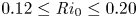 $0.12 \leq {Ri}_0 \leq 0.20$. We find a relatively small difference between
  ${Ri}_0=0.16$ and
  ${Ri}_0=0.19$ for our class T simulations, possibly less than might be expected due to the manner in which our simulations are perturbed from the point of maximal billow amplitude causing a more coherent pattern of secondary instabilities at higher
  ${Ri}_0$ than was found in Mashayek et al. (Reference Mashayek, Caulfield and Peltier2013). This manner of perturbation and subsequent emergence of secondary instabilities is also likely the reason why our values of
  $\eta _c$ for L simulations are larger than those reported in VanDine et al. (Reference VanDine, Pham and Sarkar2021). Values of
  $\eta _c^{3\text{-}D}$ are in general similar to those reported by Mashayek et al. (Reference Mashayek, Caulfield and Peltier2013), Salehipour & Peltier (Reference Salehipour and Peltier2015) and VanDine et al. (Reference VanDine, Pham and Sarkar2021), though it is important to note that reasonable differences may arise due to the precise definition being used as discussed in § 3.2. These comparisons raise an important point: the uncertainties in values of mixing efficiency resulting from minor differences in simulation set-up, as well as the choice of how mixing efficiency is defined, may be as large as reported differences that arise from modifying specific flow parameters such as
  ${Re}$ and
  ${Ri}_0$. This highlights some of the problems with using any one set of idealised numerical simulations in attempting to model complex geophysical environments.
Table 2. Cumulative values  $\chi _c$,
  $\varepsilon _c$ and the resulting mixing efficiency
  $\eta _c=\chi _c/(\chi _c+\varepsilon _c)$ calculated by integrating
  $\chi$ and
  $\varepsilon$ in time over the entire mixing event, or from the start of the fully developed 3-D turbulence (indicated by a superscript) defined as the point where
  $\varepsilon$ first reaches a local maximum. Vertical integration is performed over the region
 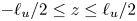 $-\ell _u/2 \leq z \leq \ell _u/2$.

By considering a locally defined APE, two possible local measures of mixing  $\chi _{{loc}}$ and
  $\tilde {\chi }_{{loc}}$ were defined that differ only in their interpretation of the background stratification. The quantity
  $\chi = \langle \chi _{{loc}} \rangle$ is often used as an alternative definition for mixing, dating back to the work of Osborn & Cox (Reference Osborn and Cox1972) who show that a corresponding diapycnal diffusivity
  $K_{\rho }$ may be calculated as
  $K_{\rho } = \chi /N^2$. Here
  $\tilde {\chi } = \langle \tilde {\chi }_{{loc}}\rangle$ is analagous to a measure of mixing proposed by Arthur et al. (Reference Arthur, Venayagamoorthy, Koseff and Fringer2017) that attempts to estimate local values of the background density profile
  $\rho _B$ by sorting individual vertical columns. For the KHI mechanism considered here, where overturnings caused by the roll-up of the billow lead to small and often negative local density gradients, we found that using
  $\chi _{{loc}}$ calculated by computing the background density gradient as a constant bulk value averaged over the shear layer generally leads to a better approximation of the precise mixing efficiency than
  $\tilde {\chi }_{{loc}}$ which depends on local density gradients, particularly whilst distinct overturnings persist in the flow. As discussed in Arthur et al. (Reference Arthur, Venayagamoorthy, Koseff and Fringer2017), the way in which
  $N^2$ is computed can impact subsequent measures of mixing; with this in mind we have demonstrated that using the distribution of local efficiencies calculated using
  $\tilde {\chi }_{{loc}}$ may provide reasonable bounds on values of the bulk mixing efficiency. Moreover, our analysis of the period in which secondary instabilities proliferate demonstrates that
  $\chi _{{loc}}$ has physical significance as a local mixing diagnostic, with large values generally bordering regions of dense APE as might be expected from the theory.
From an oceanographic point of view, the primary quantity of interest is the diapycnal diffusivity  $K_\rho$ which may be calculated in a variety of ways. As originally noted by Winters & D'Asoro (Reference Winters and D'Asoro1996), the ‘true’ diapycnal diffusivity depends on the sorted background density profile, which is in practice impossible to calculate precisely from observational data. Indeed, such a quantity is really a local measure of the flux through a given isopycnal surface in the fluid, and subsequently defined bulk measures inevitably depend on the precise averaging process used in a similar manner to the discussion surrounding definitions of local mixing in § 3.2.
Salehipour & Peltier (Reference Salehipour and Peltier2015) and Howland et al. (Reference Howland, Taylor and Caulfield2021) demonstrate that the Osborn–Cox method provides a reasonable approximation for the ‘true’ diffusivity, a conclusion that is supported in our data through the agreement of the closely related mixing efficiencies  $\eta _\chi$ and
  $\eta _{\mathscr {M}}$. However, it is important to note that even their definitions of a ‘true’ diffusivity differ in terms of the averaging process used, in the sense that
 \begin{equation} K_\rho^{{Salehipour}} \sim \frac{\langle \text{local flux}\rangle}{\langle \text{local gradient}\rangle},\quad K_\rho^{{Howland}} \sim \left\langle \frac{\text{local flux}}{\text{local gradient}}\right\rangle. \end{equation}
The comparison of mixing efficiencies in § 3.2 demonstrates that such averaging distinctions can result in appreciable differences when local gradients are highly variable, a similar conclusion to the results of Arthur et al. (Reference Arthur, Venayagamoorthy, Koseff and Fringer2017). Future work should address this issue in the context of calculated diffusivities further.
We have chosen to adopt a more practical approach and compare a variety of proposed models for diapycnal diffusivity for each of the simulations considered here. We normalise each diffusivity by a time integrated reference value
 \begin{equation} K^{T}_\rho = \frac{\int_0^{t_f}-{Ri}_0\langle{\rho'w}\rangle_T \,\textrm{d} t}{\int_0^{t_f}\langle N^2\rangle_T\,\textrm{d} t}, \end{equation}
in a manner similar to Taylor et al. (Reference Taylor, de Bruyn Kops, Caulfield and Linden2019), though we note that due to the transient nature of our simulations we expect to see significantly more variation in time-evolving measures of  $K_\rho$. Here
  $t_f$ is the time at which the bulk dissipation
  $\langle \epsilon \rangle _T$ first becomes smaller than 10 % of its maximum value (i.e. when the turbulence has decayed significantly from its peak). Figure 8 shows the variation of four models with
  $R_{OT}$,
 \begin{align} K_\rho^{\chi} = \frac{\chi}{\langle N^2\rangle_T};\quad K_\rho^O = \frac{\gamma\langle \epsilon\rangle_T}{\langle N^2\rangle_T};\quad K_\rho^D = \gamma \alpha^2 L_T^2 \langle N^2\rangle_T^{1/2},\quad K_\rho^I = \frac{CR_{OT}^{{-}4/3}\langle \epsilon\rangle_T}{\langle N^2 \rangle_T}. \end{align}
These models have been respectively proposed by Osborn & Cox (Reference Osborn and Cox1972), Osborn (Reference Osborn1980), Dillon (Reference Dillon1982) and Ijichi & Hibiya (Reference Ijichi and Hibiya2018), where  $\gamma =0.2$,
  $\alpha =0.8$ and the constant of proportionality
  $C=0.22$ corresponds to the blue line in figure 7(a).

Figure 8. Variation of various models for the parameterization of diapycnal diffusivity  $K_\rho$ defined in (4.3a–d) with the ratio of Ozmidov to Thorpe scales
  $R_{OT}$ for simulations (a) T16, (b) L10, (c) T19 and (d) L13. Each diffusivity is normalised by a time integrated reference value
  $K_\rho ^{T}$ defined in (4.2). The horizontal dashed line indicates a reference ratio of unity, whilst the vertical dashed line corresponds to the frequently used value
  $R_{OT}=0.8$ proposed by Dillon (Reference Dillon1982).
It is interesting to see that all of the diffusivities roughly converge to a value that is close to the time integrated reference value  $K_\rho ^{\textrm {T}}$ as
  $R_{OT}$ approaches a value of
  $O(1)$ which is similar to the observational value of Dillon (Reference Dillon1982). There are more significant deviations between models during the ‘young’ phase of turbulence when
  $R_{OT}$ is small, and the decaying phase as
  $R_{OT}$ grows much larger than unity. Interestingly,
  $R_{OT}=1$ corresponds to a value of
  $\varGamma = 0.22$ in the Ijichi & Hibiya (Reference Ijichi and Hibiya2018) parameterisation
  $\varGamma = CR_{OT}^{-4/3}$, very similar to the commonly used reference value of
  $\varGamma =0.2$ and the original upper bound of Osborn (Reference Osborn1980). However, as is clear from the evolution of
  $K_\rho ^O$, assuming a constant value of
  $\varGamma =\gamma =0.2$ results in values of diapycnal diffusivity that are significantly lower than estimates depending on a time-evolving mixing efficiency whilst large overturnings persist. This is in agreement with the findings of Salehipour & Peltier (Reference Salehipour and Peltier2015) for similar KHI simulations.
The Ijichi & Hibiya (Reference Ijichi and Hibiya2018) model  $K_\rho ^I$ attempts to resolve this difficulty and is seen to provide values of diffusivity that are similar to the more accurate estimate
  $K_\rho ^{\chi }$ for small values of
  $R_{OT}$, though as might be expected from figure 7(a), there are non-trivial differences between these two diffusivities at later times when the turbulence is decaying and
  $R_{OT}$ becomes large. At this point, based on the discussion in § 3.5 we believe that parameterizations of
  $\varGamma$ based on the Ellison scale
  $L_E$ rather than the Thorpe scale may be necessary to resolve these differences. From an oceanographic perspective, however, the errors from using
  $L_T$ instead of
  $L_E$ are not likely to be of leading order importance as the mixing is far weaker by this stage.
An additional notable feature of figure 8 is that the Dillon (Reference Dillon1982) model  $K_\rho ^D$ actually provides very similar values of diffusivity to
  $K_\rho ^{\chi }$, despite using a constant value of
  $\varGamma =\gamma =0.2$. This is because the error during the ‘young’ phase of turbulence is compensated for by the fact that the corresponding estimate of
  $R_{OT}=\alpha =0.8$ is an overestimate for the true value at this stage. Whilst this is perhaps fortunate here, it demonstrates that even overly simplistic mixing models (at least from a fluid dynamics point of view) may provide reasonable estimates for diffusivity provided they contain some information about the ‘age’ of the turbulent event in question. However, there are clearly more dependencies affecting the behaviour of
  $K_\rho$ than a simple relationship with
  $R_{OT}$, with non-monotonic behaviour of
  $K_\rho ^\chi$ particularly observable in figure 8(b) that is not captured by the more simplistic models of
  $K_\rho ^D$ and
  $K_\rho ^I$. Overall, in agreement with previous studies of KHI turbulence, our study suggests that, without additional knowledge of the length scales of turbulent motions in the flow or, linked to this, the mechanisms producing the turbulence, caution should be applied when using a universal constant value of
  $\varGamma = 0.2$. There is growing evidence that somewhat larger values of
  $\varGamma \sim 0.3$ appear to be typical of shear-driven mixing events for
  $R_{OT} \sim 1$, as can be seen from the dense clusters of points around these values in figure 7 and as discussed by Mashayek et al. (Reference Mashayek, Caulfield and Alford2021), suggesting that classical parameterizations may be biased towards underestimation of diffusivity due to transient turbulent overturnings caused by shear instability. As figure 8 shows, these underestimates may be improved by incorporating a simple dependence on turbulent length scales into parameterizations. We also point out that, whilst there are fewer data points for small values of
  $R_{OT}$ considerably less than 1 in our simulations, a significant amount of mixing takes place during this period and therefore neglecting the transient early stage mixing behaviour may result in further underestimates of diapycnal diffusivity over the entire mixing event. Suitably high frequency spatio-temporal observations of ocean mixing events, whilst difficult to obtain, may shed additional light on the existence and relevance of such spatio-temporally varying turbulent behaviour in real-world environments.
Data from our simulations show that, at least for the initial parameter values we consider here, the turbulence produced by KHI billows is largely generic with the influence of a far field stratification having little impact on the global mixing efficiency or the local energy dissipation. This is consistent with a picture of ocean mixing being largely dependent on the ‘history’ of the turbulence, which is strongly influenced by the specific mechanisms leading to turbulent breakdown. Howland et al. (Reference Howland, Taylor and Caulfield2020) found that mixing in a variety of forced stratified flows depends heavily on the large-scale forcing implemented in their simulations, with convective mixing mechanisms produced by gravity wave forcing more efficient than shear instabilities in a purely horizontal forcing. Future work should further explore the links between turbulence-producing mechanisms and the resulting mixing regimes that ensue, which are likely to depend on a number of physical scales and flow parameters. In order to identify these mechanisms appropriately in larger-scale flows requires knowledge of the spatial variability of the turbulence. Statistical methods such as those used in Portwood et al. (Reference Portwood, de Bruyn Kops, Taylor, Salehipour and Caulfield2016) may prove effective in characterising the state of a turbulent flow at any given time by dividing it into separate regions determined by an appropriate turbulence intensity parameter. This is particularly useful when the turbulence is intermittent or the flow is in a layered state, as seems to occur in many situations of interest (Caulfield Reference Caulfield2021). At least as far as KHI turbulence is concerned however, the similarity in behaviour across all of the simulations we perform supports the use of this mechanism as a means for parameterizing diapycnal diffusivities in the ocean (e.g. Salehipour et al. Reference Salehipour, Peltier, Whalen and MacKinnon2016b), though using data from a range of DNS studies will be important for capturing the aforementioned underlying uncertainties that may arise due to differences in simulation set-up and the precise definitions of mixing parameters invoked.
Whilst we have considered a variety of different initial flow conditions here and shown mixing to be generic for these background profiles, it is important to note that the set-up is still quite specific. Firstly, we expect that the values of  ${Ri}_0$ we choose here are likely to optimise the proliferation of secondary instabilities as was seen by Mashayek et al. (Reference Mashayek, Caulfield and Peltier2013). This (along with the fact that the Reynolds number
  ${Re}$ is suitably high) has the advantage of allowing us to neglect the phenomenon of vortex pairing which may be important for more weakly stratified flows in terms of the efficiency of the mixing produced. Secondly, whilst the modified set-up we consider in which a saturated KHI billow is perturbed to generate secondary instabilities is arguably necessary to perform a consistent initial parameter comparison, it is obviously highly idealised and whether or not these efficient mechanisms for mixing occur in the ocean is not known: even small amounts of initial noise in the background flow can noticeably arrest the development of the primary KHI billow (Brucker & Sarkar Reference Brucker and Sarkar2007; Kaminski & Smyth Reference Kaminski and Smyth2019) and may prevent the emergence of coherent secondary structures altogether. The development of these instabilities is also modified for larger values of
  ${Pr}$ more relevant to the ocean (Salehipour et al. Reference Salehipour, Peltier and Mashayek2015).
It is worth saying that regardless of these caveats, we expect our analysis of the different turbulent regimes we observe to hold as long as sufficiently large overturnings are able to form at early times in the flow, in line with similar reasoning by Mashayek et al. (Reference Mashayek, Caulfield and Peltier2017). Finally, though we have argued that, at least for the simulation set-up and initial parameter values considered here, KHI behaviour is generic in two different background environments, both profiles are still very different to realistic ocean conditions and to what degree the behaviour we observe here reflects that of oceanic mixing layers remains an open question.
Declaration of interests
The authors report no conflict of interest.
Appendix. Impact of resolution on the formation of secondary instabilities
We found the resolution in the  $x$ and
  $z$ directions (i.e. the plane of the primary billow) to be of importance for the formation of secondary instabilities on a KHI billow growing from an optimally perturbed background flow. To illustrate this, we performed three additional class T simulations at
  ${Ri}=0.16$ which are detailed in table 3, changing the resolution in the
  $x$ and
  $z$ directions, and then separately in the spanwise
  $y$ direction. Each simulation was initialised from the background flow with perturbation in the form of the FGM from the linear theory, with an additional uniform white noise perturbation of amplitude
  $10^{-3}$ added to the density and velocity fields. Figures 9(a) and 9(b) show the qualitative behaviour of the local density field at a particular time during the growth of the primary KHI billow for simulations UT16 and UT16-LRXZ, where the behaviour of UT16-LRY is omitted as it is essentially the same as UT16. The early proliferation of secondary instabilities on the primary billow in UT16-LRXZ are associated with large differences in the corresponding mixing efficiency
  $\eta _{\mathscr {M}}$ as shown in figure 9(c). This is an apparently 2-D phenomenon: changing the resolution in the spanwise direction in UT16-LRY does not affect the behaviour of these secondary instabilities and the mixing efficiency during the breakdown to turbulence is similar to UT16, though at later times there are small differences in the efficiency that arise due to numerical errors in capturing the smallest scales of motion. Further investigation using purely 2-D simulations showed that increasing the resolution in the
  $x$ and
  $z$ directions essentially delayed the onset of the purely 2-D secondary shear instabilities that can be seen in figure 9, whose existence can substantially modify the breakdown to turbulence in three dimensions as has been discussed in detail by Mashayek & Peltier (Reference Mashayek and Peltier2012a,Reference Mashayek and Peltierb). We propose that these secondary instabilities may be ‘unphysically’ perturbed before the billow reaches its saturation point by numerical truncation errors at the grid scale.
Table 3. Class, flow parameters and grid sizes for each additional DNS. All simulations shown have  ${Re}=6000$,
  ${Pr}=1$ and
  $L_y=4$. Here
  $N_x$,
  $N_y$ and
  $N_z$ are the number of grid points in the streamwise, spanwise and vertical directions, respectively, whilst
  $N_z^c$ is the number of vertical grid points in the central region
  $-5< z < 5$.


Figure 9. (a) Spanwise slices through  $y=0$ at
  $t=83$ showing contours of the density field for simulations UT16-LRXZ and UT16, as labelled in the top-right corners. (c) Time evolution of the mixing efficiency
  $\eta _{\mathscr {M}}$ for all of the simulations listed in table 3. The vertical dot–dashed line indicates
  $t=83$ in accordance with the snapshots from (a). Note that here
  $t=0$ corresponds to the time at which the background flow is perturbed with an FGM from the linear theory.
Based on the above, we argue that to perform a more consistent comparison of KHI turbulence – that is, without the time of secondary instability onset being modified by grid resolution – in conditions that facilitate the inherently 2-D secondary instabilities we observe to be important for mixing here, it is necessary to proceed as we do in the main text and start simulations by providing an additional perturbation to the primary KHI billow from a comparable reference point, which we take to be the time of billow saturation where  $\mathcal {K}_{2\text{-}D}$ is a maximum. Although the spanwise resolution is seen to be less important for the grid spacings we investigate here, we are cautious and perform the simulation of primary billow roll-up in two dimensions before adding a 3-D perturbation component at the point of billow saturation. This is reasonable as, in 3-D simulations, spanwise perturbations do not grow substantially until after the billow has saturated.
As an additional note of caution, we point out that the precise realisation of the secondary instabilities may be modified by purely computational features including the grid resolution and the perturbation field, even when forcefully perturbed in the manner described above. Whilst we do not expect this to affect the general results presented in this work, we have observed it can reasonably influence the precise behaviour and evolution of flow properties such as mixing rates and dissipation, introducing uncertainty in the computed values of mixing and mixing efficiency. However, as long as coherent secondary instabilities are able to proliferate on the primary billow during the breakdown to turbulence, we expect the values computed here to be broadly representative of the general case. Future work should address this issue in more detail, and at higher values of  ${Re}$.


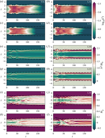


 Open access