


1. Introduction
Liquid layers subjected to an oblique temperature gradient (OTG) are encountered in microfluidics applications, additive manufacturing (Kowal, Davis & Voorhees Reference Kowal, Davis and Voorhees2018), material processing and crystal growth (Lappa Reference Lappa2010), and industrial processes such as coating and drying (Kistler & Schweizer Reference Kistler and Schweizer1997). Maintaining a purely vertical or horizontal temperature gradient in experiments studying thermocapillarity may be difficult, thus, inadvertently, a liquid layer is subjected to an OTG (Nepomnyashchy & Simanovskii Reference Nepomnyashchy and Simanovskii2009).
The Marangoni instability, named after Marangoni (Marangoni Reference Marangoni1871), arising from the temperature dependence of the surface tension and an ensuing emergence of shear stress in a liquid layer with a flat interface subjected to a purely vertical temperature gradient (VTG), was first studied theoretically by Pearson (Reference Pearson1958). He showed the emergence of the Marangoni or thermocapillary instability as a consequence of the surface-tension dependence on the temperature at the layer interface. The analysis of Pearson (Reference Pearson1958) showed that the cellular patterns observed by Bénard (Reference Bénard1901) in his pioneering experimental studies arise as a result of the Marangoni instability. Scriven & Sternling (Reference Scriven and Sternling1964), Smith (Reference Smith1966), Davis & Homsy (Reference Davis and Homsy1980) and Perez-Garcia & Carneiro (Reference Perez-Garcia and Carneiro1991) extended the study of Pearson (Reference Pearson1958) to liquid layers with a deformable surface. Here, a deformable surface refers to the liquid–gas interface with a finite surface tension whose presence allows its deformation in response, among other factors, to the tangential stresses arising due to surface-tension gradients referred to below as Marangoni stresses. Their analysis revealed a strong effect of a decrease in surface tension on the instability, which is due to a stronger temperature variation along the interface.
Another class of thermocapillary instabilities emerge due to the presence of an imposed purely horizontal temperature gradient (HTG) that affects the dynamics of a liquid layer (Davis Reference Davis1987). This setting was first theoretically investigated by Smith & Davis (Reference Smith and Davis1983a,Reference Smith and Davisb), who showed the emergence of oblique hydrothermal waves and spanwise rolls as a result of the Marangoni instability in this configuration in which the base flow is not quiescent as in the layer subjected to a VTG but flows in the direction opposite to that of the imposed HTG driven by the Marangoni stresses. Their study considered both linear and return thermocapillary flows, which refer to the flows with linear and quadratic velocity profiles with respect to the normal coordinate, respectively. The instabilities described by Smith & Davis (Reference Smith and Davis1983a,Reference Smith and Davisb) were experimentally observed by Schwabe et al. (Reference Schwabe, Moller, Schneider and Scharmann1992), Benz et al. (Reference Benz, Hintz, Riley and Neitzel1998), Riley & Neitzel (Reference Riley and Neitzel1998), Schatz & Neitzel (Reference Schatz and Neitzel2001), Ospennikov & Schwabe (Reference Ospennikov and Schwabe2004) and Schwabe (Reference Schwabe2007).
Davis (Reference Davis1987) extended the analysis of Smith & Davis (Reference Smith and Davis1983a,Reference Smith and Davisb) for a system subjected to a purely imposed HTG to the case of an imposed OTG. In the case of a fixed temperature gradient at the substrate, Davis (Reference Davis1987) showed that there exists a relationship between the critical Marangoni numbers defined using the imposed HTG and VTG, which did not predict the stabilization caused by the imposed HTG. However, the later studies of Nepomnyashchy, Simanovskii & Braverman (Reference Nepomnyashchy, Simanovskii and Braverman2001) and Shklyaev & Nepomnyashchy (Reference Shklyaev and Nepomnyashchy2004) and the present work show that a prescribed HTG has a strong stabilizing effect on the modes found by Pearson (Reference Pearson1958) which are caused by the prescribed VTG. Furthermore, Davis (Reference Davis1987) showed a negligible effect on the surface-wave instabilities at low Prandtl numbers  $Pr$. However, for moderate- and high-Prandtl-number regimes, important in practical applications involving liquids such as water with $Pr \sim 7$, Davis (Reference Davis1987) suggested a continuing effort to fill in certain gaps. The present work fills the gap of practical importance and studies the interaction between the prescribed HTG and VTG.
Inspired by the experimental limitations on imposing and maintaining a purely vertical temperature gradient and practical applications, Nepomnyashchy et al. (Reference Nepomnyashchy, Simanovskii and Braverman2001), Shklyaev & Nepomnyashchy (Reference Shklyaev and Nepomnyashchy2004), Nepomnyashchy & Simanovskii (Reference Nepomnyashchy and Simanovskii2007, Reference Nepomnyashchy and Simanovskii2009, Reference Nepomnyashchy and Simanovskii2014) and Kowal et al. (Reference Kowal, Davis and Voorhees2018) investigated the stability of liquid layers subjected to an OTG. In addition to the VTG-related stabilization of instabilities, Nepomnyashchy et al. (Reference Nepomnyashchy, Simanovskii and Braverman2001) and Shklyaev & Nepomnyashchy (Reference Shklyaev and Nepomnyashchy2004) also showed theoretically the emergence of hydrothermal waves and spanwise rolls, which could become dominant at sufficiently high HTG. The experiments of Schwabe (Reference Schwabe2007) and Mizev & Schwabe (Reference Mizev and Schwabe2009) confirmed these theoretical results.
It must be noted that Nepomnyashchy et al. (Reference Nepomnyashchy, Simanovskii and Braverman2001) and Shklyaev & Nepomnyashchy (Reference Shklyaev and Nepomnyashchy2004) studied the return flow in the layer with a non-deformable free surface. However, linear flow is important in thin films and can be experimentally realized (Schwabe Reference Schwabe2007). Furthermore, any physically realistic liquid–gas interface possesses a finite surface tension and thus the capillary number is essentially non-zero. Hence, the present study deals with linear flow generated in a liquid layer by applying an OTG to the layer with a free deformable surface. Nepomnyashchy & Simanovskii (Reference Nepomnyashchy and Simanovskii2007, Reference Nepomnyashchy and Simanovskii2009) studied the linear stability and carried out a nonlinear investigation in the framework of a thin-film approximation. However, as shown in § 4, the thin-film approximation has only partial success in capturing the impact of the imposed HTG on the instabilities related to the imposed VTG as far as the linear stability theory is concerned.
The present work investigates thermocapillary instability in a liquid layer subjected to an OTG carrying out both the general linear stability analysis (GLSA) and the nonlinear analysis in the thin-film approximation. Furthermore, weakly nonlinear stability analysis is carried out based on the thin-film approximation to understand the impact of the imposed HTG on the type of bifurcation exhibited by the film. To understand the impact of the imposed HTG on film rupture, fully nonlinear simulations around critical parameters will also be studied in the present work.
The rest of the paper is arranged as follows. The problem statement, the original governing equations and boundary conditions, the base-state fields and the governing equations for the perturbations are all introduced in § 2. The numerical technique employed in resolving the GLSA is validated in § 3 and its results are presented in § 4. The linear and nonlinear stability analyses in the framework of the long-wave approximation are carried out in § 5. The major conclusions of the present study are summarized in § 6. Finally, the pseudospectral numerical approach used in the solution of the linear eigenvalue problem for the GLSA is outlined in appendix A.
2. Problem formulation
Consider a layer of an incompressible Newtonian liquid with temperature-independent properties such as viscosity  $\mu$, density $\rho$, kinematic viscosity $\nu$ and thermal diffusivity $\kappa$ deposited upon a horizontal planar substrate in a gravitational field $g$. The layer is assumed to be of mean thickness $d$ and infinite lateral extent. The liquid layer is bounded by an ambient inert gas phase at the liquid–gas interface, which is assumed to be deformable. The coordinate system used here is Cartesian, with the $x^\ast$- and $z^\ast$-axes located in the substrate plane, whereas the $y^\ast$-axis is normal to the substrate and directed into the liquid layer, with the reference point $y^\ast =0$ located on the substrate plane. In what follows, the asterisk denotes dimensional variables, whereas their dimensionless counterparts are denoted without an asterisk.
The temperature of the planar substrate is imposed to vary in the  $x^*$-direction as $T^*_0 -\eta ^* x^*$ whereas that of the ambient gas phase is $T^*_\infty - \eta ^* x^*$, so that ${\rm \Delta} T^\ast \equiv T^*_0 - T^*_\infty >0$, where $T^*_0$ and $T^*_\infty$ are constant temperatures and $\eta ^*$ is the imposed HTG. Thus, the entire system (the substrate, the liquid layer and the gas phase) is subjected to a constant HTG in the $x^\ast$-direction. The present setting suggests that the temperature field in the liquid layer depends on both $x^\ast$ and $y^\ast$, which suggests that an OTG is imposed on the layer. As shown below in (2.7b), the base-state temperature has a cubic term in addition to the linear term in $y$. The cubic term in $y$ arises due to the presence of advection of energy. The layer is assumed to be sufficiently thin so the buoyancy effect could be neglected.
Surface tension at the liquid–gas interface  $\sigma ^*$ is assumed to be temperature-dependent,
 \begin{equation} \sigma^*=\sigma^*_0-\gamma^* (T^*-T^*_0), \end{equation}
where  $\gamma ^*=-({\textrm {d} \sigma ^*}/{\textrm {d} T^*})>0$ and $\sigma ^*_0$ is the reference surface tension of the fluid at the reference temperature of the lower plate taken as $T^*_0$. The length, time, velocity and temperature are non-dimensionalized by $d$,
$d$,  $d^2/\kappa$, $\kappa /d$ and $\beta ^* d$, respectively, where $\beta ^*$ is the imposed VTG to be specified later. Furthermore, pressure and stresses are non-dimensionalized by $\mu \kappa /d^2$.
We denote the dimensionless fluid velocity field as  $\boldsymbol {v}=(v_x,v_y,v_z)$, with $v_i$ being the velocity components in the direction $i=x,y,z$. The dimensionless continuity and momentum conservation equations are
 \begin{gather} \boldsymbol{\nabla} \boldsymbol{\cdot} \boldsymbol{v}=0, \end{gather}
 \begin{gather}\frac{1}{Pr} [ \partial_t \boldsymbol{v} + (\boldsymbol{v} \boldsymbol{\cdot} \boldsymbol{\nabla}) \boldsymbol{v} ] = - \boldsymbol{\nabla} p - G\,Pr \boldsymbol{\nabla} y + \nabla^2 \boldsymbol{v}, \end{gather}
where  $Pr={\mu }/{\rho \kappa }$ is the Prandtl number, $G={gd^3}/{\nu ^2}$ is the Galileo number, $\boldsymbol {\nabla }=(\partial _x,\partial _y,\partial _z)$ is the gradient operator, $\nabla ^2 \equiv \partial ^2_x + \partial ^2_y + \partial ^2_z$ is the Laplacian operator, $p$ is the pressure and $\partial _i$ denotes the partial derivative with respect to $i$. The dimensionless heat advection–diffusion equation is
 \begin{equation} \partial_t T + (\boldsymbol{v}\boldsymbol{\cdot}\boldsymbol{\nabla}) T = \nabla^{2} T . \end{equation}
 The governing equations (2.2) are subjected to the following boundary conditions. Assuming no slip, impermeability and a constant specified temperature at the solid substrate  $y=0$ yields
 \begin{equation} v_x=0, \quad v_y=0, \quad v_z=0, \quad T=T_0 - \eta x, \end{equation}
where  $\eta ={\eta ^*}/{\beta ^*}$ represents the dimensionless HTG. The deformable gas–liquid interface is located at $y=1+\xi (x,y,t)$, where $\xi (x,z,t)$ is the infinitesimal displacement of the interface from its undisturbed position $y=1$.
The boundary conditions at the interface are the kinematic boundary condition, the tangential and normal components of the stress balance (Perez-Garcia & Carneiro Reference Perez-Garcia and Carneiro1991) and the continuity of the heat flux, respectively,
 \begin{gather} \partial_t \xi + \boldsymbol{v}_\perp \boldsymbol{\cdot} \boldsymbol{\nabla} \xi = v_y, \end{gather}
 \begin{gather}\boldsymbol{t}_j \boldsymbol{\cdot} \boldsymbol{\tau} \boldsymbol{\cdot} \boldsymbol{n}= - Ma \boldsymbol{\nabla} T \boldsymbol{\cdot} \boldsymbol{t}_j, \end{gather}
 \begin{gather}-p + \boldsymbol{n} \boldsymbol{\cdot} \boldsymbol{\tau} \boldsymbol{\cdot} \boldsymbol{n} = -Ca^{-1} (\boldsymbol{\nabla} \boldsymbol{\cdot} \boldsymbol{n}) - Bo \, Ca^{-1} \xi, \end{gather}
 \begin{gather}\boldsymbol{\nabla} T \boldsymbol{\cdot} \boldsymbol{n}=-Bi (T-T_\infty + \eta x), \end{gather}
where
 \begin{equation} Ma=\frac{\gamma \beta^* d^2}{\mu \kappa}, \quad Bo=\frac{\rho g d^2}{\sigma_0^*}, \quad Bi=\frac{qd}{k_{th}}, \quad Ca=\frac{\mu \kappa}{\sigma_0^* d}, \end{equation}
respectively, are the Marangoni, Bond, Biot and capillary numbers, with  $Bo = G\,Ca$ and $j=1,2$. Here $q$,
$q$,  $\sigma ^*_0$, $g$ and $k_{th}$ are the coefficient of thermal convection at the free surface, the surface tension evaluated at the free surface temperature, the gravitational acceleration and the thermal conductivity of the fluid, respectively. The vectors $\boldsymbol {t}_j$ and $\boldsymbol {n}$ represent the unit tangent and unit normal vectors to the free surface, respectively. Also, the vector $\boldsymbol {v}_\perp$ is the two-dimensional vector obtained by projection of $\boldsymbol {v}$ onto the $x$–
$x$– $z$ plane, $\boldsymbol {v}_\perp =(v_x,v_z)$. The linearized expressions for the normal $\boldsymbol {n}$ and tangential $\boldsymbol {t}_1$ and $\boldsymbol {t}_2$ vectors at the free surface in the perturbed state are
 \begin{equation} \boldsymbol{n}=-\partial_x \xi \boldsymbol{e}_x + \boldsymbol{e}_y - \partial_z \xi \boldsymbol{e}_z, \quad \boldsymbol{t}_1= \boldsymbol{e}_x + \partial_x \xi \boldsymbol{e}_y, \quad \boldsymbol{t}_2= \partial_z \xi \boldsymbol{e}_y + \boldsymbol{e}_z. \end{equation}
The vectors,  $\boldsymbol {e}_x$, $\boldsymbol {e}_y$ and $\boldsymbol {e}_z$ are the unit vectors in the $x$-,
$x$-,  $y$- and $z$-directions, respectively.
2.1. Base state
For the base state, the governing equations (2.2) are subjected to the following boundary conditions. Assuming no slip, impermeability and constant temperature at the solid substrate  $y=0$ they are
 \begin{equation} \bar v_x=0, \quad \bar v_y=0, \quad \bar v_z=0, \quad \bar T=T_0 - \eta x. \end{equation}
At the undisturbed gas–liquid interface  $y=1$, the boundary conditions are the kinematic boundary condition, the tangential component of the stress balance and the continuity of the heat flux, respectively,
 \begin{gather} \bar v_y =0, \end{gather}
 \begin{gather}\frac{\textrm{d} \bar v_x}{\textrm{d} y}= - Ma\,\partial_x \bar T, \end{gather}
 \begin{gather}\partial_y \bar T=-Bi (\bar T-T_\infty + \eta x). \end{gather}
The governing equations (2.2) and boundary conditions determine the base state in the form
 \begin{gather} \bar v_x=\eta \,Ma \, y, \quad \bar v_y=0, \quad \bar v_z=0, \quad \bar p= p_a -G \, Pr \, y, \end{gather}
 \begin{gather}\bar T (x,y) = T_0-\eta x + \left[ \frac{\eta^2 Ma}{2(1+Bi)} \left( 1+\frac{Bi}{3} \right) - 1 \right] y - \frac{\eta^2 Ma}{6} y^3, \end{gather}
where
 \begin{equation} \beta^\ast = \frac{Bi {\rm \Delta} T^\ast}{(1+Bi) d}. \end{equation}
From (2.7b), the HTG induces an additional VTG, which has positive sign and counteracts the imposed negative VTG. Furthermore, the induced VTG is proportional to  $\eta ^2$. As shown later in § 4, the induced VTG has a strong effect on the Marangoni instabilities exhibited by the imposed VTG.
2.2. Perturbed state
Next, infinitesimally small perturbations are imposed on the base-state equations (2.7) to carry out the linear stability analysis of the system. Squire's theorem (Schmid & Henningson Reference Schmid and Henningson2001) is not applicable in the present case due to the imposed HTG. Thus, in what follows, three-dimensional disturbances are considered. The governing equations are then linearized around the base-state equations (2.7) and normal modes
 \begin{equation} f'(\boldsymbol{x},t)=\tilde{f}(y) \exp(\textrm{i} k x + \textrm{i} m z+s t), \quad \xi(x,z,t)=\tilde{\xi} \exp(\textrm{i} k x + \textrm{i} m z+s t) \end{equation}
are substituted into these. Here  $f'(\boldsymbol {x},t)$ is a perturbation to a dynamic quantity $f({\boldsymbol x},t )$, such as the components of the fluid velocity field $v_x$, $v_y$ and $v_z$, pressure $p$ and temperature $T$,
$T$,  $\tilde {f}(y)$ is the corresponding eigenfunction in the Laplace–Fourier space and $\tilde \xi$ is a constant. The parameters $k$ and $m$ are the wavenumbers of the perturbations in the $x$- and $z$-directions, respectively, and the value $s=s_r+\textrm {i} s_i$ is the complex growth rate. The flow is linearly unstable if at least one eigenvalue satisfies the condition $s_r>0$. As a result of this procedure, the linearized continuity, momentum conservation and energy equations become
 \begin{gather} \textrm{i}k\tilde v_x + \textrm{D}\tilde v_y + \textrm{i}m \tilde{v}_z=0, \end{gather}
 \begin{gather}\frac{1}{Pr} [ s \tilde{v}_x + \textrm{i}k \bar v_x \tilde v_x + \tilde v_y \textrm{D}\bar v_x ] = -\textrm{i}k \tilde p + (\textrm{D}^2 - k^2 - m^2) \tilde v_x, \end{gather}
 \begin{gather}\frac{1}{Pr} [ s \tilde{v}_y + \textrm{i}k \bar v_x \tilde v_y ] = -\textrm{D}\tilde p + (\textrm{D}^2 - k^2 - m^2) \tilde v_y, \end{gather}
 \begin{gather}\frac{1}{Pr} [ s \tilde{v}_z + \textrm{i}k \bar v_x \tilde v_z ] = -\textrm{i}m\tilde p + (\textrm{D}^2 - k^2 - m^2) \tilde v_z, \end{gather}
 \begin{gather}s \tilde{T} + \textrm{i}k \bar v_x \tilde T + \partial_x \bar T \tilde{v}_x + \partial_y \bar T \tilde{v}_y = (\textrm{D}^2-k^2 - m^2) \tilde T, \end{gather}
where  $\textrm {D} \equiv {\textrm {d}}/{\textrm {d} y}$.
Equations (2.10) are then supplemented with the following boundary conditions. At  $y=0$, the assumptions of no slip and impermeability at the lower plate imply
 \begin{equation} \tilde v_x=0, \quad \tilde v_y=0, \quad \tilde v_z=0, \quad \tilde T=0. \end{equation}
At the deformable boundary, due to the presence of the Marangoni forces, additional stresses are generated. Thus, upon a standard procedure of projection of the boundary conditions at the deformed interface  $y=1+\xi$ onto $y=1$, the boundary conditions at $y=1$ become
 \begin{gather} \tilde v_y=s\tilde \xi + \textrm{i}k \bar v_x \tilde \xi, \end{gather}
 \begin{gather}\tilde \tau_{xy}=-\textrm{i} k\,Ma (\tilde T + \partial_y \bar T \tilde \xi ), \end{gather}
 \begin{gather}\tilde \tau_{yz}=-\textrm{i} m\,Ma (\tilde T + \partial_y \bar T \tilde \xi ), \end{gather}
 \begin{gather}-\tilde p+\tilde \tau_{yy} - 2\textrm{i}k \textrm{D} \bar v_x \tilde\xi =-\frac{(Bo+k^2+m^2)}{Ca} \tilde \xi, \end{gather}
 \begin{gather}\textrm{D} \tilde T + Bi\,\tilde T + ( -\textrm{i}k \partial_x \bar T + \partial^2_y \bar T + Bi\,\partial_y \bar T ) \tilde \xi=0. \end{gather}
While deriving the normal stress balance boundary condition (2.11e), it has been assumed that the thermocapillary contribution to the normal stress balance is negligible, i.e.
 \begin{equation} \gamma^* (\bar T^*|_{y^*=d}-T^*_0 )/\sigma^*_0 = Ma\,Ca (\bar T|_{y=1}-T_0 ) \ll 1 . \end{equation}
Since for most liquids  $Ma\,Ca \ll 1$ at the onset of the linear instability, this assumption holds true provided that $(\bar T|_{y=1}-T_0) = O(1)$. This also helps to proceed with the normal mode analysis by removing the term $\bar T|_{y=1}$ which depends on $x$ and therefore could represent an obstacle.
Equations (2.10)–(2.11) constitute a generalized linear eigenvalue problem, which is to be solved for the eigenvalues  $s$ and the eigenfunctions for a specified set of parameter values $Bi$,
$Bi$,  $Bo$,
$Bo$,  $Ca$,
$Ca$,  $Pr$ and $Ma$. To determine the spectrum of the eigenvalue problem (2.10)–(2.11), the pseudo-spectral method is employed, the details of which are presented in appendix A.
3. Validation
Thermocapillary instability in the fluid layers subjected to OTG has been previously studied by Nepomnyashchy et al. (Reference Nepomnyashchy, Simanovskii and Braverman2001) and Shklyaev & Nepomnyashchy (Reference Shklyaev and Nepomnyashchy2004) for a return flow configuration. They considered a two-layer structure of the fluids with the fluid–fluid interface assumed to be non-deformable. Thus, a validation by using the results obtained in their studies is difficult. Instead, a three-way validation using the results obtained by Smith & Davis (Reference Smith and Davis1983a,Reference Smith and Davisb) and Hu, He & Chen (Reference Hu, He and Chen2016) for a purely HTG and Perez-Garcia & Carneiro (Reference Perez-Garcia and Carneiro1991) for a purely VTG, is presented below.
Smith & Davis (Reference Smith and Davis1983b) analysed surface-wave instabilities in a liquid layer subjected to a purely HTG. Their study revealed an absence of long-wave instabilities in the flow considered here, which they referred to as ‘linear flow’ due to its base-state velocity profile. The present non-dimensionalization format does not allow the limit of a purely HTG. Thus, to validate our numerical approach, the linearized perturbation equations of Smith & Davis (Reference Smith and Davis1983b) were directly used in the code. The additional dimensionless numbers in their study were the surface-tension number,  $S=\rho d \sigma ^*_0/\mu ^2$, and the Reynolds number, $Re=Ma/Pr$. The agreement between the data extracted from a representative neutral stability curve in the study of Smith & Davis (Reference Smith and Davis1983b) along with that obtained by using our numerical approach is shown in figure 1. The results presented in figure 1 show an excellent agreement between Smith & Davis (Reference Smith and Davis1983b) and the present numerical approach, thereby validating the latter.

Figure 1. Neutral stability curves in  $k$–
$k$– $Re$ space for the problem corresponding to curve (b) in figure 1 of Smith & Davis (Reference Smith and Davis1983b). An excellent agreement between the data extracted from Smith & Davis (Reference Smith and Davis1983b) and our numerical approach shown by the dot-dashed curve and circles, respectively, validates the latter.
Smith & Davis (Reference Smith and Davis1983b), however, did not present the eigenspectrum; thus, to achieve an independent validation for our numerical technique, the eigenspectrum obtained using the latter is compared with Hu et al. (Reference Hu, He and Chen2016) in table 1. It must be noted that Hu et al. (Reference Hu, He and Chen2016) studied the instabilities in an Oldroyd-B liquid layer subjected to a purely HTG with a non-deformable surface. Additionally, our numerical approach predicts the critical Marangoni number  $Ma_c =15.49$ and the critical wavenumber $k_c= 0$ for $Bi=0$ and $Pr=\infty$ for the emergence of longitudinal stationary rolls in a liquid layer subjected to a purely HTG, which is in a perfect agreement with Smith & Davis (Reference Smith and Davis1983a).
Table 1. The four leading eigenvalues in the eigenspectrum for a liquid layer subjected to a purely HTG obtained using our numerical approach and those taken from Hu et al. (Reference Hu, He and Chen2016) with  $Pr=0.02$, $Ma=6.15$, $k=0.0251676$, $m=0.389187$, $Bo=0$, $Bi=0$ and $Ca=0$. The agreement between the two columns validates our numerical technique.

Smith & Davis (Reference Smith and Davis1983a,Reference Smith and Davisb) and Hu et al. (Reference Hu, He and Chen2016) studied the instabilities arising due to the purely imposed HTG, but, in the present problem, an additionally imposed VTG is also present. The non-dimensionalization scheme here allows for the existence of a purely VTG, and the governing equations for this problem can be simply obtained by substituting  $\eta =0$ into the set of equations (2.10) and into the base state (2.7a) and (2.7b). Similarly, the numerical solution for the OTG can be reduced to the case of a purely VTG.
The previous studies of Scriven & Sternling (Reference Scriven and Sternling1964), Davis & Homsy (Reference Davis and Homsy1980) and Perez-Garcia & Carneiro (Reference Perez-Garcia and Carneiro1991) on the Marangoni instability in a liquid layer with a deformable interface subjected to a purely VTG demonstrated the predominant emergence of the stationary mode characterized by  $s_i=0$, implying non-travelling disturbances at the onset of instability. The neutral stability curve for the stationary mode with $\eta =0$ and $m=0$ can be obtained analytically by substituting $s=0$ into the governing equations (2.10)–(2.11) and solving the corresponding eigenvalue problem in terms of the Marangoni number $Ma$ in the form (Scriven & Sternling Reference Scriven and Sternling1964)
 \begin{equation} Ma=-\frac{8 k (Bo + k^2) [ k \cosh(k) + Bi \sinh(k) ] [k - \cosh(k) \sinh(k)]}{-k^3 [Bo + (1 - 8 Ca) k^2] \cosh(k) + (Bo + k^2) \sinh^3(k)}. \end{equation}
 It can be immediately deduced from (3.1) that the neutral Marangoni number and its critical value (if the instability is indeed stationary)  $Ma_c$ are independent of $Pr$. It must be noted that, for a Newtonian liquid with temperature-independent density, only the stationary mode of the Marangoni instability was theoretically predicted (Perez-Garcia & Carneiro Reference Perez-Garcia and Carneiro1991). The variation of $Ma$ with $k$ given by (3.1) is presented in figure 2 for a fixed set of parameters. The parameter $Ma_c$ is obtained by minimizing $Ma(k)$, and the critical wavenumber $k_c$ is determined then via $Ma_c= Ma(k_c)$.

Figure 2. Variation of  $Ma$ with $k$ for the stationary mode in a liquid layer with $Bi=0$, $Bo=0.1$, $\eta =0$ and $Ca=0.01$. The figure also presents a validation of our numerical approach. The continuous curve is obtained from the analytical expression (3.1), whereas the triangles are obtained numerically. The system is unstable for $Ma$ in the domain above the curve.
For the stationary mode with  $Bi=0$, $Bo=0.1$ and $Ca=0.01$, the critical Marangoni number $Ma_c=6.6667$, as obtained by Perez-Garcia & Carneiro (Reference Perez-Garcia and Carneiro1991) is in agreement with the value of $Ma_c$ obtained from (3.1). To validate our numerical approach, the neutral stability curves determined both via (3.1) and numerically are presented in figure 2, which exhibits an excellent agreement between the two.
4. Results and discussion
4.1. General linear stability analysis
Before proceeding with the results, it is important to determine the limits of the parameter values to be used hereafter. The ranges for the dimensional parameters are  $d \sim 10^{-6}\text {--}10^{-3}$ m, $\rho \sim 10^{3}$ kg m $^{-3}$, $\gamma \sim 10^{-5}\text {--}10^{-3}$ N m K $^{-1}$, $k_{th} \sim 10^{-6}\text {--}10^{-3}$ J m $^{-1}$ s $^{-1}$ K $^{-1}$, $q \sim 1\text {--}10^{2}$ J m $^{-2}$ s $^{-1}$ K $^{-1}$, $\kappa \sim 10^{-7}\text {--} 10^{-5}$ m $^2$ s $^{-1}$, $\mu \sim 10^{-3}\text {--}10^{2}$ Pa s and $\sigma _0^* \sim 10^{-3}\text {--}10^{-1}$ N m $^{-1}$ (Ezersky et al. Reference Ezersky, Garcimartin, Mancini and Perez-Garcia1993; Li, Xu & Kumacheva Reference Li, Xu and Kumacheva2000; Ospennikov & Schwabe Reference Ospennikov and Schwabe2004; Mizev & Schwabe Reference Mizev and Schwabe2009), and the corresponding dimensionless numbers are $Bi \sim O(10^{-3}\text {--}10)$, $Bo \sim O(10^{-3}\text {--}10^{-1})$, $Ca \sim O(10^{-4}\text {--}10^{-1})$ and $Pr \sim O(1\text {--}10^3)$. This parametric range will be used in the present study to analyse various modes of instability.
The eigenvalue spectrum for the present problem with a chosen parameter set is illustrated in figure 3 showing a set of converged eigenvalues. We refer to the eigenvalues as converged if they vary only at the sixth significant digit upon variation in the number of collocation points  $N$ from $N=50$ to $N=75$. For a purely VTG, only stationary, either stable or unstable, modes exist. However, the thermocapillary convection induced by an imposed HTG converts these stationary modes to the convective ones, i.e. modes with $s_i \neq 0$, as illustrated in figure 3(a).

Figure 3. The eigenspectrum of the present problem for  $Bi=0$, $Bo=0.1$, $Pr=7$, $\eta =0.05$, $Ma=90$, $k=m=0.01$ and $Ca=0.001$ illustrating the shift of the stationary modes from stationary ( $s_i=0$) to convective ( $s_i \neq 0$) modes. (a) The full spectrum along with the line at $s_i=-0.0225$, which is a consequence of the HTG. (b) The magnified spectrum of the two leading eigenvalues, with the most unstable one originating from the stationary mode of the purely VTG, which now becomes a downstream ( $s_i<0$) mode as a consequence of the imposed HTG. In both panels, the overlap of the eigenvalues obtained for $N=50$ and $N=75$ shows their genuine nature.
The position of the vertical line along which most of the eigenvalues are clustered in figure 3(a) can be explained as follows. The eigenspectra for plane Couette, plane Poiseuille and Hagen–Poiseuille flows show a similar vertical line at the average base-state speed multiplied by the wavenumber of the disturbance (Schmid & Henningson Reference Schmid and Henningson2001). The average base-state velocity in the present case is  $\eta Ma/2$, which is also the phase speed of the wave; thus the frequency of the perturbations ( $-s_i$) travelling with this speed becomes $k\eta Ma/2$. For the parameter set used in figure 3, the estimate above yields $s_i=-0.0225$, which is in a perfect agreement with the vertical line shown in figure 3. This also implies that $s_i=0$ for $\eta =0$, which is indeed the case since $s_i=0$ for all modes when a liquid layer is subjected to a purely VTG. As a consequence of the imposed HTG, the stationary instability mode with $s_r \sim 0.02$ becomes a downstream ( $s_i<0$) mode, as shown in figure 3(b).
The spanwise long-wave ( $k=0$) unstable mode remains stationary, in contrast with the oblique ( $k\neq 0,\ m\neq 0$) or streamwise ( $m=0$) long-wave modes. This may be a consequence of the absence of the flux due to the base state in the $z$-direction similar to the flux in the $x$-direction induced by the HTG component of the applied OTG.
Along with the long-wave modes, the present analysis also reveals the emergence of a new class of unstable modes. The evolution of the two unstable modes from this class of modes in the eigenspectrum of the problem with an increase in  $Ma$ is shown in figure 4. These new modes were not found in the earlier studies of Scriven & Sternling (Reference Scriven and Sternling1964), Perez-Garcia & Carneiro (Reference Perez-Garcia and Carneiro1991) and Patne, Agnon & Oron (Reference Patne, Agnon and Oron2020), where a liquid layer was subjected to a purely VTG. The existence of such modes in the present analysis thus stems from the interaction between the imposed VTG and the thermocapillary flow induced by the imposed HTG. The new modes satisfy $s_i<0$, and thus they represent downstream modes. The neutral stability curves for the streamwise and spanwise long-wave modes and the new mode are illustrated in figure 5. For the long-wave modes, even with $\eta \neq 0$, the critical wavenumbers are $k_c$ and/or $m_c=0$. Thus, the long-wave instability existing for a purely VTG is not affected by the presence of the thermocapillary flow.

Figure 4. The evolution of the two leading eigenvalues with an increase in  $Ma$, which results in the emergence of the new modes of instability. The parameters here are $Bi=0$, $Bo=0.1$, $Pr=7$, $\eta =1$, $Ma=90$, $k=0.3$, $m=0.0$ and $Ca=0.001$. These new modes originate as a result of the interaction between the imposed HTG and VTG components, and these modes can only exist if the OTG is imposed and the free surface is deformable.

Figure 5. Neutral stability curves presenting the variation of  $Ma$ with $k$ for the stationary mode in a liquid layer for $Bi=0$, $Bo=0.1$, $Pr=7$ and $Ca=0.01$ for the streamwise and spanwise long-wave modes and the new short-wave mode. For the latter, the critical wavenumbers are $k_c \approx 0.38$ and $m_c=0$, so its neutral stability curve is determined for $m=0$. The base flow is unstable for $Ma$ greater than the boundary set by the respective curves.
With  $\eta =0$ and the parameter sets shown in figure 5, (3.1) yields $Ma_c=6.667$; however, the neutral stability curves presented in figure 5 yield $Ma_c=7.19$. Thus, irrespective of the streamwise or spanwise character of the long-wave modes, the stabilizing effect of the imposed HTG is the same as that of the HTG on the instabilities introduced by the purely VTG, which could be explained via the following argument: The term $[{\eta ^2 Ma}/(2(1+Bi))] (1+{Bi}/{3}) - 1$ in the base-state temperature (2.7b) shows that the imposed HTG introduces a VTG that counteracts the imposed VTG, effectively weakening it, thereby stabilizing the long-wave deformational instabilities introduced by the latter. The neutral stability curve for the new mode has a minimum at $k_c=0.38$, and thus it is a finite-wavelength mode.
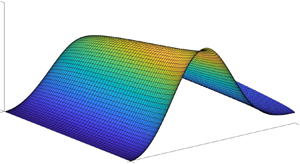
The perturbed fields of the fluid velocity components  $v^\prime _x$ and $v^\prime _y$ and temperature $T^\prime$ corresponding to the marginally stable new mode at the critical parameters are shown in figure 6. The critical parameters correspond to the minimum on the neutral stability curve for the new mode in figure 5. These perturbations have been normalized by their respective maximal absolute values. The velocity perturbations are essentially non-zero at the free surface as a consequence of the Marangoni effect driving the instability at the layer interface. However, due to the presence of an OTG, the temperature perturbations exhibit the maximal value at $y\approx 0.45$. This maximal value exhibited by the temperature perturbations is sensitive to the variation in the strength of the HTG, $\eta$. For example, for $\eta =4$ with the same parameter set as in figure 6(c), the maximum of the temperature perturbation takes place at $y \approx 0.5$. Furthermore, at higher values of $\eta$, the temperature perturbation field exhibits multiple extrema in the domain $y\in [0,1]$.

Figure 6. The normalized perturbation fields (a)  $v'_x$, (b) $v'_y$ and (c) $T'$ for $Bi=0$, $Bo=0.1$, $Pr=7$, $\eta =1$, $Ma=22.62$, $k=0.38$, $m=0.0$ and $Ca=0.01$ for the marginally stable eigenvalue $s=-17.86566\textrm {i}$. Here, $v'_x=\textrm {Re}[ \tilde v_x \,\textrm {e}^{\textrm {i}kx} ]$, $v'_y=\textrm {Re}[ \tilde v_y \,\textrm {e}^{\textrm {i}kx} ]$ and $T'=\textrm {Re}[ \tilde T \,\textrm {e}^{\textrm {i}kx} ]$. The length of the domain in the $x$-direction is equal to the wavelength of the perturbations, $2{\rm \pi} /k$. For convenience, the axes are normalized to the interval $[0,1]$. The velocity perturbations attain their maximal values at the free surface due to the presence of the Marangoni stresses. However, the temperature perturbation field attains its maximum at $y \sim 0.45$ due to the imposed OTG.
Figure 7 presents the critical curve in the plane spanned by the value of  $\eta$ and the critical Marangoni number $Ma_c$. For $Ca=0.01$ and a purely VTG, only the long-wave deformational mode of the instability exists (Perez-Garcia & Carneiro Reference Perez-Garcia and Carneiro1991; Patne et al. Reference Patne, Agnon and Oron2020). Upon imposing an OTG, however, the long-wave mode is confined to the region $\eta <0.2$ for sufficiently large Marangoni numbers $Ma$. This confinement leads to the formation of an instability island presented in figure 7. As explained above, the term $\{[{\eta ^2 Ma}/(2(1+Bi))] (1+{Bi}/{3}) - 1\} y$ in the base-state temperature (2.7b) suggests that the imposed HTG induces a VTG proportional to $[{\eta ^2 Ma}/(2(1+Bi))] (1+{Bi}/{3})$ which counteracts the imposed VTG, thereby stabilizing the long-wave mode. This suggests that when both, an imposed VTG and an induced VTG are of the same strength, the long-wave instability disappears, implying that the quantity $[{\eta ^2 Ma}/(2(1+Bi))] (1+{Bi}/{3})-1$ must vanish. This procedure for $Bi=0$ leads to $Ma_c=2/\eta ^2$, which is also the line shown in figure 7. As expected, the instability island of the long-wave mode in the $\eta$– $Ma$ plane lies below this asymptote, as seen in figure 7(a). The upper boundary of the instability island can be approximated by the line $Ma_c=1/\eta ^2$. Although not shown here, a similar stabilizing effect is also observed for either the spanwise or an oblique long-wave mode, and the critical values $Ma_c$ are exactly the same as that for the streamwise long-wave mode.

Figure 7. Variation of the critical Marangoni number  $Ma_c$ with $\eta$ for $Bi=0$, $Bo=0.1$, $Pr=7$ and (a) $Ca=0.01$ and (b) $Ca=0.0001$. For the new mode in panels (a) and (b), the critical wavenumber is $k_c \sim 0.38$ and $0.22$, respectively. The new mode exhibits characteristic scaling $Ma_c \sim 1/\eta$ for $\eta > 0.3$. The dashed line $Ma_c =2/\eta ^2$ represents a borderline beyond which the long-wave deformational mode is suppressed for $Bi=0$.
For a relatively strong surface tension, e.g.  $Ca=0.0001$, the finite-wavelength mode with $k_c=1.98$ and $Ma_c=79.6$ exists for the imposed purely VTG (Pearson Reference Pearson1958). Similar to the long-wave mode, the imposed HTG also stabilizes the finite-wavelength mode, since the stabilizing effect discussed above also acts upon the finite-wavelength disturbances, as shown in figure 7(b). In contrast with the long-wave mode, the finite-wavelength mode does not form an island of instability; instead, it crosses the barrier asymptote $Ma_c=2/\eta ^2$ and continues as one of the instability modes from the class of new modes. Since its critical Marangoni number is larger than that of the new mode, it then becomes the second most unstable mode, thereby losing its importance as the dominant mode of instability.
The new mode of instability found in the present work exhibits a characteristic scaling  $Ma_c \sim 1/\eta$ with the critical wavenumber $k_c$ that does not vary with $\eta$ for $\eta > 0.3$. Also, the critical spanwise wavenumber for the new mode is found to be zero, and thus it is a streamwise mode of instability. Since the long-wave mode is confined to $\eta <0.2$ for $Ca=0.01$, as seen in figure 7(a), and the finite-wavelength mode is confined to $\eta < 0.1$ for $Ca=0.0001$, as shown in figure 7(b), then the new mode governs the stability of the system in the range to the right of the tip of the instability island. Thus, the imposed HTG may suppress the instabilities related to the VTG, but it leads to the emergence of new instability modes. This implies that the imposed HTG does not necessarily have a stabilizing effect on the system, in contrast with the previous studies (Nepomnyashchy et al. Reference Nepomnyashchy, Simanovskii and Braverman2001; Shklyaev & Nepomnyashchy Reference Shklyaev and Nepomnyashchy2004). The continuation of the finite-wavelength mode also falls under the class of new modes whose critical Marangoni number scales as $Ma_c \sim 1/\eta$.
Extension of the new modes presented in figure 7 into the domain  $\eta <0.1$ turns out to be a numerically difficult task. The difficulty arises because the long-wave mode, due to a much lower value of $Ma_c$ as compared to that of the new mode, becomes unstable over a large range of $k$, thereby making it hard to track the new mode by using the numerical technique employed here. Also, the new mode does not represent the dominant instability mode for low values of $\eta$; hence a further analysis of the new mode in that domain is not carried out.
The effects of variations of  $Bo$ and $Pr$ on the critical parameters of the system are shown in figure 8. Figure 8(a) shows that an increase in the Bond number, equivalent to an increase of the relative importance of gravity with respect to capillarity, leads to a shrinkage of the instability island for the long-wave mode, whereas it has a negligible effect on the critical parameters for the new mode. The reason for this is that the Bond number $Bo$ appears only in the normal-stress boundary condition (2.11e) in combination with the two wavenumbers as $Bo+k^2+m^2$. Thus, only if the critical wavenumbers are of the same order of magnitude as the Bond number can the latter affect the critical parameters of the corresponding instability mode. For the long-wave mode $k_c=m_c\sim 0$, and thus it is readily affected by the variation in $Bo$, whereas the new mode with $k_c \sim 0.4$ is negligibly affected for small $Bo$. On physical grounds, this implies that long-wave disturbances are more affected by gravity as compared to those of a finite wavelength. As for variation in the Prandtl number $Pr$ with a fixed $Bo$, the influence on the long-wave and the new modes is opposite to that of $Bo$, as shown in figure 8(b), namely the long-wave mode remains almost unaffected, whereas the short-wave new mode is more sensitive. An increase in $Pr$ leads to a decrease in the strength of the inertial terms that play a crucial role in introducing the new modes, as explained in § 4.3, which explains the stabilization caused by an increase in $Pr$.
$Pr$.

Figure 8. Variation of  $Ma_c$ with $\eta$ at $Bi=0$ and $Ca=0.01$. (a) The effect of varying $Bo$ on $Ma_c$ for $Pr=7$. (b) The effect of varying $Pr$ on $Ma_c$ for $Bo=0.1$. The critical wavenumber is negligibly affected by variation of $Bo$ and $Pr$.
$Pr$.
At high values of  $\eta$, along with the new modes, the spectrum of the problem contains also pairs of unstable spanwise modes. For $k=0$, the spanwise modes form pairs of eigenvalues with equal growth rate and absolute value of the oscillation frequency but travelling in opposite directions. Two such pairs, one unstable and one stable, are illustrated in figure 9(a). As the wavenumber $k$ increases, the symmetry of the modes with respect to the sign of $s_i$ breaks, as shown in figure 9(b). An increasing $k$ favours the downstream mode, which continues as the most unstable mode among the class of new unstable modes discussed above, while the growth rate of the upstream mode decreases with an increase in $k$, thereby emphasizing its spanwise nature. For an arbitrary value of $\eta$, the new mode always has a lower $Ma_c$ as compared to the spanwise mode; thus a further analysis of the spanwise mode will not be carried out. Also, the second unstable mode, which is a new one shown in figure 4, emerges from the downstream mode of the second pair shown in figure 9(a).

Figure 9. The spectra for  $Bi=0$, $Bo=0.1$, $Pr=7$, $\eta =10$, $Ma=4$, $m=0.5$ and $Ca=0.01$. (a) The emergence of a pair of unstable symmetric spanwise eigenvalues at $k=0$ with an equal growth rate but corresponding to propagation in the opposite directions at the same phase speed. (b) The symmetry is broken for values of $k \neq 0$. With an increase in $k$, the growth rate of the downstream mode increases, whereas that of the upstream mode decreases. The downstream mode is the new mode of instability when tracked by slowly varying the values of the wavenumbers $k$ and $m$.
$m$.
4.2. Energy analysis
To explain the effect of the imposed OTG on the thermocapillary instabilities, the following discussion analyses the effect of the imposed HTG on the perturbation energy balance. In what follows, the approach of Hu, Peng & Zhu (Reference Hu, Peng and Zhu2013) and Hu et al. (Reference Hu, He and Chen2016) has been followed. Before proceeding, the Navier–Stokes equations (2.2b) linearized around the base state  $\bar {\boldsymbol {v}}$ are recast as
 \begin{equation} \frac{1}{Pr} \frac{\partial \boldsymbol{v}^\prime}{\partial t} = -\boldsymbol{\nabla} p^\prime + \boldsymbol{\nabla} \boldsymbol{\cdot} \boldsymbol{\tau}^\prime - \frac{1}{Pr} [ (\boldsymbol{v}' \boldsymbol{\cdot} \boldsymbol{\nabla}) \bar{\boldsymbol{v}} + ( \bar{\boldsymbol{v}} \boldsymbol{\cdot} \boldsymbol{\nabla}) \boldsymbol{v}' ], \end{equation}
where the quantity  $\boldsymbol {\tau }^\prime$ is the disturbance of the stress tensor for a Newtonian fluid. Taking the scalar product with the perturbation velocity vector ${\boldsymbol {v}}^\prime$, integrating the result over the flow domain and simplifying the resulting integrals yields an equation describing the time evolution of the total kinetic energy of the perturbations,
 \begin{equation} E = \tfrac{1}{2} \int{ {\boldsymbol{v}}^\prime \boldsymbol{\cdot} {\boldsymbol{v}}^\prime\,\textrm{d} V},\end{equation}
in the form
 \begin{align} \frac{1}{Pr} \frac{\partial E}{\partial t} &= -\int\! p^\prime \boldsymbol{v}^\prime \boldsymbol{\cdot} \boldsymbol{n} \,\textrm{d} A - \frac{1}{2} \int\! \boldsymbol{\tau}^\prime \boldsymbol{:} \dot{\boldsymbol{\gamma}}^\prime \,\textrm{d} V + \int \! \boldsymbol{\tau}^\prime \boldsymbol{\cdot} \boldsymbol{v}^\prime \boldsymbol{\cdot} \boldsymbol{n} \,\textrm{d} A -\frac{1}{Pr} \int \! \boldsymbol{v}' \boldsymbol{\cdot} \bar{\dot{\boldsymbol{\gamma}}} \boldsymbol{\cdot} \boldsymbol{v}' \,\textrm{d} V \nonumber\\ &\equiv -I_p - I_b + I_M - I_R, \end{align}
where  $I_p$, $I_b$, $I_M$ and $I_R$ are the components of pressure work, the bulk stress work, the surface stress work (Marangoni stress work) and the Reynolds stress work (Drazin Reference Drazin2002) in the energy balance, respectively. The quantities, $\textrm {d} V$ and $\textrm {d} A$ are the volume and area elements, respectively, and the area integrals are over the flow domain boundary. The quantities $\dot {\boldsymbol {\gamma }}^\prime = \boldsymbol {\nabla } \boldsymbol {v}^\prime + \boldsymbol {\nabla } {\boldsymbol {v}^\prime }^\textrm {T}$ and $\bar {\dot {\boldsymbol {\gamma }}} = \boldsymbol {\nabla } \bar {\boldsymbol {v}} + \boldsymbol {\nabla } \bar {\boldsymbol {v}}^\textrm {T}$ represent the strain-rate tensors associated with the perturbed and base states, respectively. Since it is only at the free deformable surface that the velocity perturbations ${\boldsymbol {v}}^\prime$ do not vanish, the contribution to the area integrals will come from the free surface alone. Sample values of the integrals in (4.3) are shown in table 2. The Marangoni stress work component $I_M$ of (4.3) is found to be positive for the parameter values explored here, and thus it exerts a destabilizing effect. The bulk stress work component $I_b$ is unconditionally positive in the case of a Newtonian fluid, since $\boldsymbol {\tau }^\prime \boldsymbol {:} \dot {\boldsymbol {\gamma }}^\prime = \gamma '_{ij}\gamma '_{ji} \ge 0$, and thus leads to a decrease in the perturbation energy due to the presence of viscous dissipation. Note that stationary modes for $\eta =0$ may still emerge even if the bulk stress work integral is positive. These stationary modes may become unstable by virtue of the Marangoni stress work and the pressure work integral $I_p$, which is found to be negative for the parameter range studied here.
Table 2. Sample values of the pressure work  $I_p$, bulk stress work $I_b$ and Reynolds stress work $I_R$ integrals normalized by the value of the Marangoni stress work integral $I_M$ for $Bi=0$, $Bo=0.1$, $Ca=0.01$ and $Pr=7$ for the unstable stationary long-wave (the first two rows) and the new (the last two rows) modes. The bulk stress work remains positive as expected and thus has a stabilizing effect due to viscous dissipation. Since both the pressure work and Reynolds stress work integrals are negative, these components of the energy balance result in the growth of the perturbation energy. The contribution of the Reynolds stress work is much smaller compared to the rest of the components.

The integral  $I_R$ is a volume-averaged correlation between the perturbations in the horizontal and vertical components of the velocity field. This term is also responsible for the energy exchange between the base state and perturbation quantities. Upon simplification for the present problem, it reduces to $2 \eta Ma \, v'_x v'_y$ which turns out to be negative for the parameter range studied here, as shown in table 2. Thus, Reynolds stress work has a destabilizing effect, but it may be subdued at high $Pr$ and low $\eta$. It is also seen from table 2 that, since all values are normalized with respect to the Marangoni stress work term, the contribution of the latter to the energy balance is major with respect to those of the other components. The bulk stress work becomes on a par with the Marangoni stress work as far as its absolute value is concerned when the value of $\eta$ increases. To summarize, except for the bulk stress work, all other components of the energy balance lead to the growth of the disturbance energy.
4.3. Physical mechanism
This section is devoted to a discussion of the physical mechanisms driving the instabilities revealed in the previous sections. The Marangoni stresses exerted on the free surface of the layer give rise to the base-state flow with a non-zero velocity profile under the assumption that  $\eta \neq 0$. These base-state flow components then provide coupling with perturbations at the free surface, which leads to the exchange of energy between the base state and the perturbations, eventually causing the instabilities observed here. However, a physical mechanism of the emerging instabilities and their stabilization predicted here might give a better understanding of the underlying processes.
In the case of the Marangoni instability due to the purely imposed VTG, the physical mechanism can be described as follows (Smith Reference Smith1986; Davis Reference Davis1987). Thermal perturbations at the layer free surface may lead to the emergence of a hot spot and, due to the Marangoni stresses arising from the variation in temperature-dependent surface tension, liquid parcels at the surface flow away from the hot spot. However, to maintain mass conservation, a vertical flow develops from underneath the free surface towards it. The fluid beneath the free surface is hotter than at the surface itself as a result of the imposed VTG. Thus, convective heat flux triggered by the upflow generated by the hot spot warms it up even more, enhancing the conductive heat flux, thereby making the liquid layer unstable provided that dissipative effects due to liquid viscosity and thermal diffusivity do not cause decay of the driving mechanism.
The suppression of the instability driven by the VTG via the prescribed HTG revealed in the present paper can be explained in the following way. The imposed HTG induces a VTG and the latter turns out to counteract the imposed VTG. Thus, if a hot spot emerges at the liquid–gas interface due to thermal fluctuations, while the imposed VTG leads to a decrease in the temperature as one moves away from the bottom wall, the induced VTG leads to the opposite effect. Thus, even if a hot spot emerges, the upwelling flow generated due to the mass conservation may not bring the energy sufficient to compensate the heat loss due to the heat conduction from the hot spot if the induced VTG is sufficiently high. Hence, to suppress the instability caused by the imposed VTG, the induced VTG must be of a comparable magnitude to inhibit the warming up of the hot spot. To have this happen quantitatively, the coefficient of  $y$ in the base-state temperature (2.7b) must vanish, which in turn leads to the asymptote $Ma \sim 2/\eta ^2$.
The physical mechanisms responsible for the emergence of the instabilities observed due to the imposed purely HTG were explained by Smith (Reference Smith1986). The new class of instability modes lie in the region where the imposed HTG dominates the imposed VTG and these modes emerge at finite critical wavenumbers  $k_c$. The importance of inertia in the emergence of the new instability modes can be immediately noticed from figure 8(b), which shows that a decrease in inertia equivalent to an increase in $Pr$ has a strong stabilizing effect. Following the above discussion, consider a hot spot generated as a result of thermal perturbations at the interface. Driven by the Marangoni stresses, the fluid will then flow from this hot spot towards the nearest cold spots, while to conserve mass, upflow takes place. However, this upflow brings a colder fluid to the hot spot since the magnitude of the induced opposing VTG is greater than that of the imposed VTG owing to the existence of the new modes above the asymptote $Ma_c \sim 2/\eta ^2$. Thus, the hot spot may lead to heat loss by both conduction and convection (due to cold upwelling flow), thereby stabilizing the fluctuations. However, before the upflow can cool off the hot spot, the thermocapillary flow driven by the imposed HTG carries the energy of the hot spot downstream, thereby preventing cooling it by the upflow since the interface has the maximal velocity.
As said, to prevent stabilization by cooling from underneath due to the upwelling flow, the base-state velocity at the free surface must be sufficiently large, and thus these new modes do not exist at low  $\eta$. The hot-spot perturbations then interact with the base-state flow and temperature through the inertial terms of the momentum conservation and energy equations. Thus, the original hot spot fades away while a new hot spot emerges downstream, which may offset the heat loss by conduction and the upflow, eventually leading to the instability revealed in this paper. The role played by the interaction terms between the base state and the perturbations can also be inferred from table 2, where the rightmost column represents the Reynolds stress integral $I_R$ of (4.3) quantifying the energy transferred from the base state to the field of perturbations. Thus, an increase in $I_R$ leads to an increase in the energy transfer from the base state to the perturbations, thereby destabilizing the flow and giving rise to the new mode of instability.
Although the imposed VTG component does not play a major role in the emergence of the new instability modes, it reduces the cooling effect due to the upflow by counteracting the induced VTG. Thus, the imposed HTG component plays a major role in the emergence of the new instability modes, while the imposed VTG component sustains their generation.
5. Long-wave analysis
In this section, we derive the long-wave evolution equation describing the nonlinear dynamics of a thin liquid film subjected to an OTG. We then carry out linear and weakly nonlinear analyses of the system followed by numerical solution of the fully nonlinear evolution equation to support the results of the latter. Following the standard procedure (Oron, Davis & Bankoff Reference Oron, Davis and Bankoff1997), the wavelength of the disturbances  $L$ is assumed to be substantially larger than the average thickness of the film $d$, where $d=\epsilon L$ and $\epsilon \ll 1$.
To derive the thin-film evolution equation, the following scaling transformation is used in (2.2):  $x \to X\epsilon ^{-1}$, $y \to y$, $t \to \tau \epsilon ^{-1}$, $v_x \to U$, $v_y \to \epsilon V$, $T \to T$ and $p \to \varPi \epsilon ^{-1}$. The local instantaneous film thickness $h^*(x^*,t^*)$ is normalized by $d$, i.e. $h^*=hd$. Using these scalings, at the leading order $O(\epsilon ^0)$ the governing equations (2.2) reduce to
 \begin{equation} -\partial_X \varPi + \partial^2_y U=0,\quad \partial_y \varPi = G Pr,\quad \partial^2_y T=0.\end{equation}
Equations (5.1a–c) are supplemented with the following boundary conditions. At the substrate  $y=0$, the assumptions of no slip, no penetration and an imposed temperature imply
 \begin{equation} v_x=0, \quad v_y=0, \quad T=-\hat{\eta} X, \end{equation}
where  $\hat {\eta }=\eta \epsilon ^{-1}$ is the scaled imposed HTG. At the free surface $y=h(x,t)$, the continuity of the tangential and normal stresses and Newton's cooling law yield, respectively,
 \begin{gather} \partial_y U=-\widehat{Ma}\,\partial_X T, \end{gather}
 \begin{gather}\varPi=-\widehat{Ca}^{-1} \partial^2_X h + \hat{G} Pr \,h, \end{gather}
 \begin{gather}\partial_y T + Bi (T+ \widehat{{\rm \Delta} T}+\hat{\eta} X) = 0, \end{gather}
where
 \begin{equation} \widehat{Ma}=\epsilon Ma,\quad \widehat{Ca}=\epsilon^{-3}Ca,\quad \hat{G} = \epsilon G, \quad \widehat{{\rm \Delta} T} = \frac{T_0^* - T_\infty^*}{\beta^* d},\end{equation}
respectively, are scaled Marangoni, capillary and Galileo numbers, while  $\widehat {{\rm \Delta} T}$ is the dimensionless temperature difference between the substrate and free surface temperatures.
The solution of the  $O(\epsilon ^0)$ equations (5.1a–c) along with the boundary conditions (5.3) yields
 \begin{equation} U = \left( \frac{y^2}{2} - y h \right) \partial_X \varPi + \widehat{Ma} \left[ \eta + \frac{1+Bi}{(1+Bi \, h)^2} \partial_X h \right]y. \end{equation}
The kinematic boundary condition at the free surface in its conservative version yields, in terms of the non-dimensional film thickness  $h(x,t)$,
 \begin{equation} \partial_\tau h = -\partial_X \int_0^h U \,\textrm{d} y, \end{equation}
and upon substitution of (5.5) into (5.6) this results in
 \begin{equation} \partial_\tau h = \partial_X \left[ \frac{h^3}{3} \partial_X \varPi - \widehat{Ma} \frac{h^2}{2} \left( \eta + \frac{1+Bi}{(1+Bi \, h)^2} \partial_X h \right) \right], \end{equation}
where the pressure  $\varPi$ is given by (5.3b).
The first, second and third terms of (5.3b) account for the impact of the capillarity and gravity, HTG and VTG, respectively. Now scaling back the quantities in the above equation yields
 \begin{equation} \partial_t h = \partial_ x \left[ \frac{h^3}{3} \partial_ x ( -Ca^{-1} \partial_x^2 h + Bo \, Ca^{-1} h ) - Ma \frac{h^2}{2} \left( \eta + \frac{1+Bi}{(1+Bi \, h)^2} \partial_x h \right) \right]. \end{equation}
Equation (5.8) is therefore the evolution equation governing the nonlinear dynamics of a thin film subjected to an OTG and represents the key equation in the forthcoming study. Note a slight difference between the coefficient of the last term of (5.8) containing  $1+Bi$ instead of the conventional $Bi$ in the same term – see, for instance, (2.63) in Oron et al. (Reference Oron, Davis and Bankoff1997). The difference is due to normalization of temperature with an imposed VTG component instead of the temperature difference between those of the substrate and the ambient gas. Next, linear and weakly nonlinear stability analyses of the system are carried out based of the evolution equation (5.8).
5.1. Linear stability analysis
To study the linear stability of the system, we substitute  $h(x,t)=1+h^\prime (x,t)$ into (5.8) with $h^\prime (x,t) \ll 1$ as a perturbation imposed on the film interface. The resulting expression is then linearized about the unperturbed height in which normal modes of the form $h^\prime (x,t) =\tilde {h}\exp (\textrm {i}kx+st)$ with a constant $\tilde {h}$ are used and the dispersion relation in terms of the complex growth rate $s$ is obtained as
 \begin{equation} s = \frac{1}{6} k \left[-\frac{2k(Bo + k^2)}{{Ca}} - 6\textrm{i}\eta Ma + \frac{3Ma\,k}{(1 + Bi)} \right].\end{equation}
 The real and imaginary parts of the complex growth rate  $s$ yield the growth rate and frequency of the critical disturbances, respectively, as
 \begin{equation} s_r = \frac{1}{6}k^2\left[-\frac{2(Bo + k^2)}{{Ca}} + \frac{3Ma}{(1 + Bi)} \right], \quad s_i = -\eta k\, Ma.\end{equation}
The fastest-growing linear mode  $k=k_m$ is determined by finding the value of $k$ where a maximum for the growth rate $s_r$ given by (5.10a,b) is obtained:
 \begin{equation} k_m = \frac12 \sqrt{\frac{3 Ma \,Ca}{1+Bi}- 2 Bo}.\end{equation}
The corresponding wavelength is thus
 \begin{equation} L_m= \frac{2{\rm \pi}}{k_m}.\end{equation}
 It is immediately clear from (5.10a,b) that the long-wave approximation does not predict stabilization of the long-wave mode in contradiction with the corresponding result obtained in the general linear stability analysis presented in the previous section. As discussed there, the VTG induced by the imposed HTG counteracts the imposed VTG, thereby leading to the stabilization of the long-wave mode. The induced VTG originates from the convective terms of the base state of the heat advection–diffusion equation. However, in the thin-film approximation, the convective terms of the heat equation, i.e. the third equation in (5.1a–c), are of order higher than  $O(\epsilon ^0)$, and therefore their contribution is absent in the leading-order evolution equation. The inability of the thin-film analysis to predict the stabilizing effect of the HTG explains the reason why it is missing in the analysis carried out by Nepomnyashchy & Simanovskii (Reference Nepomnyashchy and Simanovskii2007, Reference Nepomnyashchy and Simanovskii2009). This also implies the necessity for the general linear stability analysis performed and presented above. The expression for $s_i$ in (5.10a,b) suggests an advection of the disturbances introduced by the imposed HTG in agreement with the results of the GLSA.
It follows from (5.9) that the growth rate of the disturbances is independent of the imposed HTG, and thus the result shown in figure 10(a) is valid for arbitrary  $\eta$. The instability sets in with an increase in $Ma$ beyond the critical value $Ma=Ma_{c}$.

Figure 10. Variation of (a) the growth rate  $s_r$ and (b) the frequency $s_i$ with the disturbance wavenumber $k$ as obtained from (5.9) for $Bi=0.01$, $Bo=0.1$ and $Ca=0.01$. (a) Destabilization of the film with an increase in the Marangoni number for an arbitrary value of $\eta$. The critical value of the Marangoni number in this case is $Ma_{c}=6.6667$. (b) Variation of the frequency of the disturbances with $\eta$ at $Ma=15$. The negative value of $s_i$ indicates the downstream propagation of the long-wave mode for a non-zero $\eta$. For $\eta =0$, there is no propagation.
The expression for the critical Marangoni number  $Ma_{c}$ in the case of a film of infinite extent ( $k \to 0$) is obtained from (5.10a,b) by setting the growth rate $s_r$ to zero:
 \begin{equation} Ma_{c}= \frac{2(1+Bi) Bo}{3Ca}. \end{equation}
If the characteristic length  $L$ of the film in the horizontal direction is finite, the critical value of the Marangoni number is altered accordingly to account for this feature:
 \begin{equation} Ma_{c}= \frac{2 (1+Bi) \left[Bo+(2{\rm \pi}/L)^2\right]}{3Ca}. \end{equation}
With  $\eta =0$, the critical wavenumber is $k_c=0$ for the long-wave mode, and thus taking the limit $k \rightarrow 0$ in (3.1) and simplification of the resulting expression leads to (5.13). Thus, the critical Marangoni number given by the thin-film approximation is in agreement with that obtained from the GLSA for $\eta =0$. A comparison of $Ma_c$ obtained from the GLSA and the thin-film analysis is shown in figure 11. For a low strength of the imposed HTG, both the GLSA and the long-wave approximation are in a very good agreement.

Figure 11. Variation of the critical Marangoni number  $Ma_c$ with $\eta$ as obtained from the GLSA and the long-wave analysis for $Bi=0$, $Bo=0.1$, $Pr=7$ and $Ca=0.01$. At low $\eta$, the GLSA is in agreement with the long-wave analysis.
5.2. Weakly nonlinear analysis
It is known that a thin film subjected to a VTG along with capillarity and stabilizing gravity with ensuing Marangoni stresses undergoes subcritical bifurcation (vanHook et al. Reference vanHook, Schatz, Swift, McCormick and Swinney1997; Oron & Bankoff Reference Oron and Bankoff1999; Alexeev & Oron Reference Alexeev and Oron2007). To carry out the weakly nonlinear stability analysis in the case at hand, we follow the approach of Oron & Bankoff (Reference Oron and Bankoff1999) and Cheng, Chen & Lai (Reference Cheng, Chen and Lai2001) and introduce slow time scales  $T_1=\delta t$ and $T_2=\delta ^2 t$, where $\delta \ll 1$ is a small parameter related to the deviation of the Marangoni number from its critical value:
 \begin{equation} \delta = \frac{Ma-Ma_{c}}{Ma_{c}}. \end{equation}
 The Marangoni number  $Ma$ and the film thickness $h(x,t)$ are expanded into series of $\delta$ as
 \begin{gather} Ma=Ma_{c} (1 + \delta + \delta^2 + \delta^3 + \cdots), \end{gather}
 \begin{gather}h(x,t) = 1+ \delta h_1 (x,t,T_1,T_2) + \delta^2 h_2 (x,t,T_1,T_2)+\delta^3 h_3 (x,t,T_1,T_2)+\cdots, \end{gather}
and these are substituted into (5.8) after the latter is multiplied by  $(1+Bi \, h)^3$, eliminating by this the denominators in various terms and bringing the equation into ‘polynomial form’ to simplify the forthcoming analysis. The problem is solved order by order in $\delta$.
At first order in  $\delta$, the correction to the film thickness $h_1$ due to the perturbations is obtained in the form $h_1 (x,t,T_1,T_2)= a(T_1,T_2) \exp (\textrm {i} (k_c x + s_i t)) + \text {c.c.}$, where $a(T_1,T_2)$ is the complex amplitude of the perturbation, yet unknown, evolving in slow time and c.c. denotes complex conjugate.
At second order in  $\delta$, a linear differential equation in terms of the temporal growth rate of the amplitude $a(T_1,T_2)$ in slow time scale $T_1$ is obtained. The growth rate obtained at second order in $\delta$ is due to the normal modes, since the solution of the differential equation turns out to be exponential, similar to $h_1$ above, namely $h_2 (x,t,T_1,T_2)= b(T_1,T_2) \exp (\textrm {i} (k_c x +s_i t)) + \text {c.c.}$, with the complex amplitude $b(T_1,T_2)$ proportional to $a(T_1,T_2)^2$.
Finally, at third order in  $\delta$, the Landau equation governing the temporal evolution of the amplitude function $a \equiv a(T_1,T_2)$ in slow time $T_2$ is obtained,
 \begin{equation} \partial_{T_2} a=\lambda_1 a - \lambda_2 |a|^2 a,\end{equation}
where  $\lambda _1$ and $\lambda _2$ are the Landau parameters:
 \begin{equation} \lambda_1=-\frac{4 \textrm{i} k_c [ 2 (1 + Bi)^2 \eta + \textrm{i} Bi \, k_c ] Ma_c }{8 Bi (1 + Bi)}, \quad \lambda_2 = \frac{c_1 c_4 - 3 c_2 c_3}{c_4 c_5}, \end{equation}
with  $k_c=2 {\rm \pi}/L$ the cut-off wavenumber and $Ma_c$ the critical value of the Marangoni number obtained from $s_r=0$ for $k=k_c$, and $s_i = -\eta k Ma_c$. The constants $c_i,\ i=1,\ldots ,5$, are given by
 \begin{equation} \left.\begin{aligned} c_1 & = -4 (1 + Bi) \{k_c [2 (1 + 2 Bi (4 + 5 Bi)) k_c (Bo + k_c^2) \\ & \quad - Ca (-6 \textrm{i} Bi (1 + 2 Bi) \eta + k_c + 9 Bi \,k_c) Ma_c] + 6 \textrm{i} Bi^2 Ca \,s_i\}, \\ c_2 & = k_c \{2 (1 + Bi) (2 + 3 Bi) k_c (Bo + k_c^2) + Ca [2 \textrm{i} (1 + Bi) (1 + 4 Bi) \eta \\ & \quad - (4 + 3 Bi) k_c] Ma_c\} + 6 \textrm{i} Bi (1 + Bi) Ca \,s_i,\\ c_3 & = k_c \{2 (1 + Bi) k_c [Bo + 6 Bi \,Bo + (7 + 24 Bi) k_c^2] \\ & \quad + Ca [2 \textrm{i} (1 + Bi) (1 + 4 Bi) \eta - (2 + 15 Bi ) k_c] Ma_c\} + 6 \textrm{i} Bi (1 + Bi) Ca\, s_i,\\ c_4 & = k_c [2 (1 + Bi) k_c (Bo + 4 k_c^2) + 3 \textrm{i} Ca (\eta + Bi \,\eta + \textrm{i} k_c) Ma_c ] \\ & \quad + 3 \textrm{i}(1 + Bi) Ca \,s_i,\\ c_5 & = 8 (1 + Bi)^3 Ca. \end{aligned} \right\} \end{equation}
 For a film subjected to Marangoni stresses induced by a purely VTG, namely  $\eta =0$, the Landau equation (5.17a) is real, the cubic coefficient $\lambda _2$ is negative and bifurcation from equilibrium is subcritical. Also, note that, in the case of $\eta =0$, the coefficient $\lambda _1$ contains $k_c^2$ as a factor. The latter is positive if the cut-off wavenumber exists, i.e. the system is linearly unstable, and it is negative if the system is linearly stable, i.e. $k_c$ does not exist since $k_c^2<0$.
In the case of  $\eta \neq 0$, the Landau equation (5.17a) is complex. For sufficiently low values of $\eta$, the real part of $\lambda _2$ is negative, $\lambda _{2r}<0$, as shown in figure 12. This implies that the temporal evolution according to (5.17a) is super-exponential, so the disturbances will go on increasing for $Ma > Ma_c$, leading to film rupture and the formation of dry spots. However, figure 12 also shows that, at sufficiently high $\eta$, the Landau coefficient $\lambda _2$ satisfies the condition $\lambda _{2r}>0$; therefore, bifurcation is then supercritical. As a consequence, the temporal evolution of $a$ leads to saturation of the interface disturbance and the emergence of a stationary continuous interfacial shape. The effects of $Bi$,
$Bi$,  $Bo$ and $Ca$ on the value of $\lambda _{2r}$ are illustrated in figure 12. It is interesting to note that, as $\eta$ tends to zero, the value of $\lambda _{2r}$ tends to a constant negative value.

Figure 12. Variation of  $\lambda _{2r}$ with the parameter $\eta$ demonstrating the change in the bifurcation type for the periodic domain of $L= L_m \approx 141.197$, showing the effect of: (a) varying Bond number $Bo$, with $Bi=0.01$ and $Ca=0.001$; (b) varying Biot number $Bi$, with $Bo=0.1$ and $Ca=0.001$; and (c) varying capillary number $Ca$, with $Bi=0.01$ and $Bo=0.1$. The critical value of $Ma_c$ for these parameters is obtained using (5.14).
Variations of the Bond number  $Bo$, the Biot number $Bi$ and the capillary number $Ca$ have strong effects on the value of $\lambda _{2r}$, which also suggests that the bifurcation changes its type from subcritical to supercritical with an increase in $\eta$. For sufficiently low values of $\eta$, i.e. when the relative strength of the HTG is low, the film undergoes subcritical bifurcation, $\lambda _{2r} <0$. However, depending on the other parameters, at a particular $\eta$, $\lambda _{2r}$ becomes positive and the film bifurcates supercritically from the equilibrium.
The implications of these results are as follows: The vertical component of the imposed OTG leads to thermocapillary flow and increasing interfacial deformation, which tends to rupture the film. The horizontal component of the imposed gradient induces flow in the  $x$-direction. This flow brings liquid into the thinning part of the film, and the thinning process may be weakened or even halted if the rate of filling in is sufficiently fast. The transition of the bifurcation from subcritical for lower values of $\eta$ to supercritical for larger $\eta$ supports this observation. The subcritical bifurcation suggests an unbounded increase in the amplitude of the interfacial deformation which results in film rupture, whereas supercritical bifurcation yields a halt in the amplitude growth and therefore amplitude saturation. Hence, a careful control of the imposed HTG could be used in manipulating the emergence of the dry spots.
Figure 13 presents the results of the numerical investigation of (5.8) in a long periodic domain of length  $L=L_m \approx 141.197$ (equivalent to $\epsilon =0.007$) for the Marangoni number $Ma=70$ near its critical value $Ma_c=68.667$ for $Ca=0.001$, $Bo=0.1$ and $Bi=0.01$. We stress that the full numerical study of (5.8) is not within the scope of the current paper. It is focused here only on the illustration of the film dynamics near criticality. Equation (5.8) is solved with periodic boundary conditions in the domain $0 \le x \le L$ and with the initial condition $h(x,t=0)= 1+ 0.05 \cos (2 {\rm \pi}x/L)$. The numerical approach used here is similar to that described in detail by Haimovich & Oron (Reference Haimovich and Oron2010) with a uniform grid with 1000–2000 grid points and the time step of $O(10^{-3})$.

Figure 13. Spatiotemporal evolution of the film for  $Ma=70$, $Bo=0.1$, $Bi=0.01$ and $Ca=0.001$ for various values of $\eta$ in the periodic domain corresponding to the wavelength of the fastest-growing linear mode $L=L_m \approx 141.197$. Curves 1–4 correspond to $\eta =0.005$, $0.02$, $0.03$ and $0.05$, respectively. (a) Phase plane portraits describing temporal variation of the local film thickness at $x=0$ following the transient period. The closed character of all curves suggests that they depict interfacial travelling waves propagating in the positive $x$-direction. Here $h_t$ represents the time derivative at the location $x=0$. Each of the contours shown here represents at least $10$ full loops around the periodic domain. (b) Snapshots of the interfacial shape $h(x)$. Curves 1–4 display interfacial travelling waves $h(x)$ at $t=12\,000$, $5000$, $5000$ and $12\,000$, respectively; curve 5 shows the interfacial shape $h(x)$ for $\eta =0.001$ near rupture at $t \approx 518.5$.
In the case of  $\eta =0$, for $Ma>Ma_c$ the film is linearly unstable and its spatiotemporal evolution results in its rupture, namely at a specific location within the periodic domain the instantaneous film thickness approaches zero, $h\ll 1$. When the left–right symmetry is broken by introducing an HTG and hence $\eta \neq 0$, a flow to the right emerges. With sufficiently low values of $\eta$ the flow is weak and the film rupture remains the only scenario that takes place in the long-time range. Curve 5 in figure 13(b) shows the shape of the interface $h(x)$ near the moment of rupture in the case of $\eta =0.001$. The trough of the interface displays multiple satellite drops, which are reminiscent of a sequence of fingering events discussed in Boos & Thess (Reference Boos and Thess1999) and Oron (Reference Oron2000). The difference between the pattern shown here by curve 5 in figure 13(b) and the patterns shown in Boos & Thess (Reference Boos and Thess1999) and Oron (Reference Oron2000) is the absence of symmetry induced by the flow along the $x$-axis. It is important to emphasize that (Boos & Thess Reference Boos and Thess1999) used the original hydrodynamic equations to solve the problem numerically, whereas (Oron Reference Oron2000) employed the long-wave theory to do that. It is also noteworthy that the approach to rupture is moderately slow in the absence of van der Waals force. Should the attractive van der Waals force be taken into consideration, once the film has sufficiently thinned, the process of rupture would be fast. If a repulsive van der Waals force were included in the model, the film would not rupture, and an ultrathin ‘adsorbed’ layer would form in the trough on the microscopic scale. In any case, from the macroscopic point of view, the film will rupture.
With an increase in the value of  $\eta$, the flow along the $x$-axis intensifies, the film saturates, the minimal thickness of the film stays away from zero and rupture is prevented. Figure 13(a,b) display, respectively, the phase plane portraits of the evolution past the transient period and the interfacial shapes in the long-time limit. Curves 1–4 in both panels correspond to $\eta =0.005$, $0.02$, $0.03$ and $0.05$, respectively. As follows from the phase plane portraits of the time history of the local film thickness taken at $x=0$ for the four flows, each of them reaches the state of a travelling wave propagating to the right without a change in its shape. The interfacial shapes presented in figure 13(b) are taken at large times which are due to a slow spatiotemporal evolution of the film arising from a small supercriticality $\delta \approx 0.02$. Note that similar features of flows, namely rupture for small tilt angles and saturation for larger tilt angles, was observed in the case of the film falling on the underside of a planar substrate tilted with respect to the horizontal in the gravitational field (Oron & Rosenau Reference Oron and Rosenau1992).
The weakly nonlinear analysis presented above predicts the transition from subcritical bifurcation to supercritical bifurcation for the given parameter set at  $\eta =\tilde \eta \approx 0.03354$, as demonstrated in figure 12(c). The results presented here show a qualitative agreement between the threshold of the change in the type of bifurcation and the results of the numerical solution of the nonlinear evolution equation (5.8).
We find that, on the one hand, the fully nonlinear analysis based on numerical solution of (5.8) indicates that the transition from rupture for small values of  $\eta$ and the emergence of continuous saturated states of the system takes place between $\eta =0.001$ and $\eta =0.005$ for the chosen parameter set. On the other hand, the weakly nonlinear analysis predicts the transition value at $\eta = \tilde \eta$, which in the considered case is at $\tilde \eta \approx 0.03354$. Below this value the bifurcation is subcritical,and therefore an indefinite growth of the interfacial amplitude culminating in film rupture is expected, and above it, the bifurcation is supercritical, and the growth of the interfacial deformation is saturated. Note that this apparent mismatch arises from the fact that the weakly nonlinear analysis is carried out on small deviations from equilibrium, whereas the eventual saturation of the interfacial shape takes place when the deformation of the interface is large and sometimes at the stage where the film is near rupture.
It is interesting to note that the transition value  $\eta =\tilde \eta$ arising from the weakly nonlinear analysis and also the transition value of $\eta = \bar \eta$ separating the ruptured and continuous saturated regimes as determined from the numerical solution of the evolution equation (5.8) increase with an increase in the length of the periodic domain $L$ for the parameter set of figure 13. It is found that, similar to the case of $L=L_m$ mentioned and explained above, $\bar \eta < \tilde \eta$.
We note that trajectories 2 and 4 on the phase plane portraits in figure 13(a) each display a small closed loop, whereas curve 3 features two such loops. All of these correspond to secondary dimples on the corresponding shape of the interfacial wave in figure 13(b).
We also note that, despite the fact that the cases shown in figure 13 are near criticality, there exists a large difference between the temporal period  $T$ of the travelling waves obtained numerically and presented here and the value obtained from the linear stability analysis, $|L_m/(s_i/k)| = L_m/(Ma \eta )$, which is $\approx 2.017/\eta$ for the example presented in figure 13. The values of $T$ obtained numerically for the cases presented by curves 1–4 are $705.0$, $129.0$, $106.6$ and $66.25$, respectively.
6. Conclusions
In the present study, we consider the Marangoni instability in a liquid layer with a deformable interface subjected to the presence of an oblique temperature gradient (OTG). We carry out the general linear stability analysis (GLSA) of the system and also both the linear and weakly nonlinear stability analyses in the framework of the thin-film approximation. We reveal the stabilizing effect of the horizontal component of the imposed temperature gradient (HTG) on the instabilities driven by the vertical component of the imposed temperature gradient (VTG), and demonstrate the existence of a new class of instability modes which are a consequence of the interaction between the two aforementioned components of the imposed temperature gradients.
The predicted stabilization of the long-wave instability imposed by the VTG is due to an additional VTG induced in the base state by the imposed HTG counteracting the imposed VTG. This feature leads to the formation of an island of instability in the  $\eta$– $Ma_c$ plane, where $\eta$ denotes the ratio between the components of the imposed HTG and VTG. For sufficiently high values of $\eta$, a new class of instability modes originate due to the interaction between the imposed VTG and the thermocapillary flow driven by the imposed HTG. This new class of modes exhibit characteristic scaling $Ma_c \sim \eta ^{-1}$ and $k_c \sim \mathrm {const.}$ In the region characterized by the dominance of the HTG, these modes are responsible for the instability.
A decrease in the Bond number ( $Bo$) leads to the widening of the instability island caused by the long-wave instability in the $\eta$– $Ma_c$ plane but has a negligibly small effect on the new class of modes. In contrast, a decrease in the Prandtl number $Pr$ leads to a reduction in the critical value $Ma_c$ for the new class of modes; the instability island of the long-wave instability is negligibly affected.
The linear stability analysis in the framework of the thin-film approximation does not reveal stabilization of the long-wave instability, in contradiction with the GLSA, which is due to the absence of the induced VTG component by the imposed HTG at the relevant order in the thin-film analysis. This disagreement between the GLSA and the thin-film analysis could probably be remedied by stepping up in the order of the thin-film approximation.
To further understand the role of the imposed HTG on the dynamics of the thin film beyond the linear stability theory, a weakly nonlinear stability analysis is carried out. It reveals the transition of the bifurcation type from subcritical in the absence of, or in the presence of, a weak imposed HTG to supercritical in the presence of a stronger HTG. This suggests the possibility of utilizing the HTG in manipulation of thin films and prevention or mitigating dry spot formation. Numerical solution of a pertinent nonlinear evolution equation supports the results of the weakly nonlinear stability analysis and shows the emergence of film rupture, travelling stationary and non-stationary waves.
Appendix A. Details of the numerical approach
To carry out the linear stability analysis of the problem at hand, the pseudo-spectral method is employed in which the eigenfunctions are expanded into series of Chebyshev polynomials. For convenience, the domain  $0 \le y \le 1$ is transformed into $-1 \le y \le 1$ by stretching $y \rightarrow 2y-1$.
The eigenfunctions for the perturbed velocity, pressure and temperature fields in (2.10)–(2.11) are expanded in terms of Chebyshev polynomials as
 \begin{equation} \left.\begin{gathered} \tilde v_x(y)=\sum_{m=0}^{m=N} a_m T_m (y), \quad \tilde v_y(y)=\sum_{m=0}^{m=N} b_m T_m (y), \quad \tilde v_z(y)=\sum_{m=0}^{m=N} c_m T_m (y), \\ \tilde p(y)=\sum_{m=0}^{m=N} d_m T_m (y), \quad \tilde T(y)=\sum_{m=0}^{m=N} e_m T_m (y), \end{gathered}\right\} \end{equation}
where  $T_m(y)$ are Chebyshev polynomials of degree $m$ and $N$ is the highest degree of the polynomial in the series expansion or equivalently the number of collocation points. The coefficients $a_m$, $b_m$, $c_m$ and $g_m$ are the unknowns to be solved for. The expansion series for the derivatives of the eigenfunctions are simply obtained by taking the derivative of the series as, for instance,
 \begin{equation} D\tilde v_x(y)=\sum_{m=0}^{m=N} a_m \textrm{D} T_m (y), \end{equation}
where  $\textrm {D}=\textrm {d}/\textrm {d} y$ is the differentiation operator. Similar expansions are written for the rest of the dependent variables in (A 1) as well. All series expansions are then substituted into the governing equations. For example, the discretized form of the $x$-momentum balance equation (2.10b) is
 \begin{align} & \frac{1}{Pr} \left[ (s+ \textrm{i}k \bar v_x )\sum_{m=0}^{m=N} a_m T_m (y) + \textrm{D}\bar v_x \sum_{m=0}^{m=N} b_m T_m (y) \right] \nonumber\\ &\quad =- \textrm{i}k \sum_{m=0}^{m=N} d_m T_m (y) + \sum_{m=0}^{m=N} a_m \textrm{D}^2 T_m (y) - (k^2+m^2) \sum_{m=0}^{m=N} a_m T_m (y). \end{align}
The remaining governing equations are then discretized in a similar manner.
The boundary conditions (2.11a) at the solid substrate, i.e.  $y=-1$, become
 \begin{gather} \sum_{m=0}^{m=N} a_m T_m (-1)=0, \quad \sum_{m=0}^{m=N} b_m T_m (-1)=0, \quad \sum_{m=0}^{m=N} c_m T_m (-1)=0, \end{gather}
 \begin{gather}\sum_{m=0}^{m=N} e_m T_m (-1)=0. \end{gather}
There are five boundary conditions at the free surface, one of which is utilized to eliminate the amplitude of the perturbed location of the free surface  $\tilde {h}$. Here the normal stress balance boundary condition (2.11e) is solved for $\tilde h$, which yields an expression for $\tilde \xi$ in terms of the perturbed pressure and normal stress component
 \begin{equation} \tilde h = -\frac{Ca}{Bo+k^2+m^2 - 2\textrm{i}k Ca \,\textrm{D} \bar v_x} (-\tilde{p}+ 2 \textrm{D} \tilde v_y). \end{equation}
Equation (A 6) is then substituted into the rest of the boundary conditions. The kinematic boundary condition now yields
 \begin{equation} \tilde{v}_x + (s+\textrm{i}k \bar v_x) \frac{Ca}{Bo+k^2+m^2 - 2\textrm{i}k Ca \,\textrm{D} \bar v_x} (-\tilde{p}+2 \textrm{D} \tilde v_y)=0, \end{equation}
and upon substitution of the Chebyshev series expansion into it, this results in
 \begin{equation} \sum_{m=0}^{m=N} a_m T_m (1) + \frac{Ca (s+\textrm{i}k \bar v_x)}{Bo+k^2+m^2 - 2\textrm{i}k Ca \,\textrm{D} \bar v_x} \left( -\sum_{m=0}^{m=N} d_m T_m (1)+ 2\sum_{m=0}^{m=N} b_m \textrm{D}T_m (1) \right) =0. \end{equation}
A similar procedure is then followed for the rest of the boundary conditions at the free surface  $y=1$.
The generalized eigenvalue problem is then constructed in the form
 \begin{equation} {\boldsymbol{\mathsf{A}}}\boldsymbol{e} + s {\boldsymbol{\mathsf{B}}}\boldsymbol{e}=0, \end{equation}
where  ${\boldsymbol{\mathsf{A}}}$ and ${\boldsymbol{\mathsf{B}}}$ are the matrices obtained from the discretization procedure explained above and $\boldsymbol {e}$ is the vector containing the coefficients of all series expansions (A 1).
In these matrices, each eigenfunction corresponds to an  $N \times N$ block, so $\tilde {v}_x$ occupies the first $N$ rows and columns, the second eigenfunction $\tilde v_z$ occupies the next $N$ rows and columns from $N+1$ to $2N$, and so on. Thus, matrices ${\boldsymbol{\mathsf{A}}}$ and ${\boldsymbol{\mathsf{B}}}$ are of order $5N \times 5N$.
Further details of the discretization of the governing equations and boundary conditions, and of the construction of the matrices  ${\boldsymbol{\mathsf{A}}}$ and ${\boldsymbol{\mathsf{B}}}$ can be found in the standard procedure described by Canuto et al. (Reference Canuto, Hussaini, Quarteroni and Zang1987), Gottlieb & Orszag (Reference Gottlieb and Orszag1987), Trefethen (Reference Trefethen2000) and Schmid & Henningson (Reference Schmid and Henningson2001). Next, we use the MATLAB routine polyeig to solve the constructed generalized eigenvalue problem (A 9). To filter out the spurious modes from the numerically computed spectrum of the problem, the latter is obtained for $N$ and $N+2$ collocation points, and the eigenvalues are compared with a specified tolerance, e.g. $10^{-4}$. The genuine eigenvalues are verified by increasing the number of collocation points by $25$ and monitoring the variation of the obtained eigenvalues. Whenever the eigenvalue does not change up to a prescribed precision, e.g. to the sixth significant digit, the same number of collocation points is used to determine the critical parameters of the system. In the present work, $N=75$ is found to be sufficient to achieve convergence and to determine the leading most unstable eigenvalue within the investigated parameter range.
Acknowledgements
This research was supported by the Grant 356/18 from the Israel Science Foundation (ISF). R.P. was partially supported by the Technion Funds Postdoctoral Fellowship. Y.A. was partially supported by the Millstone/St. Louis Chair in Civil and Environmental Engineering. A.O. was partially supported by the David T. Siegel Chair of Fluid Mechanics.
Declaration of interests
The authors report no conflict of interest.


 Open access