


1. Introduction
Swimming microorganisms or artificial microswimmers, driven by various self-propelling mechanisms, display rich and complex dynamic features relative to passive particles when immersed in a Newtonian fluid. For instance, the alga Chlamydomonas reinhardtii, swimming forward through its two flagella, undergoes an unusual ‘run-and-tumble’ motion in the dark, owing to its flagellar switching between synchronous and asynchronous beating (Polin et al. Reference Polin, Tuval, Drescher, Gollub and Goldstein2009). The bacteria Bacillus subtilis exhibits striking collective behaviours associated with hydrodynamic interactions when oxygen is available. They can power submillimetre gears with their asymmetric teeth to rotate in the direction of the teeth's slanted edges (Sokolov et al. Reference Sokolov, Apodaca, Grzybowski and Aranson2009). The same active organisms were also found to self-organize into a single vortex and form a steady unidirectional circulation in a cylindrical chamber, with unexpected observations of the resultant fluid flows moving in the opposite direction (Lushi, Wioland & Goldstein Reference Lushi, Wioland and Goldstein2014; Wioland, Lushi & Goldstein Reference Wioland, Lushi and Goldstein2016). The self-assembly behaviours of motile Escherichia coli were observed and successfully adopted to generate a unidirectional rotation of nanofabricated objects (also termed bacterial ratchet motors in Di Leonardo et al. (Reference Di Leonardo, Angelani, Dell'Arciprete and Di Fabrizio2010)). The same microorganisms (E. coli) were also found to exhibit circular trajectories adjacent to surfaces and be able to sense the surface slip on the nanoscale (Hu et al. Reference Hu, Wysock, Winkler and Gompper2015). More interestingly, Drescher et al. (Reference Drescher, Leptos, Tuval, Ishikawa, Pedley and Goldstein2009) reported a ‘dancing’ behaviour pattern for two algal Volvox colonies swimming close to a wall. The two Volvox colonies initially attracted each other, and then performed a ‘waltz’ or ‘minuet’ around one another (Drescher et al. Reference Drescher, Leptos, Tuval, Ishikawa, Pedley and Goldstein2009). The unusual behaviour exhibited by microorganisms swimming in viscous environments raises several issues associated with fluid dynamics. Concerning this, a series of review papers (Pedley & Kessler Reference Pedley and Kessler1992; Lauga & Powers Reference Lauga and Powers2009; Koch & Subramanian Reference Koch and Subramanian2011; Elgeti, Winkler & Gompper Reference Elgeti, Winkler and Gompper2015; Saintillan Reference Saintillan2018) focusing on different aspects of microorganisms or engineering microswimmers swimming in fluids is recommended.
Classical squirmer models (Lighthill Reference Lighthill1952; Blake Reference Blake1971a,Reference Blakeb) have been widely adopted to describe representative microorganisms (e.g. B. subtilis, C. reinhardtii, E. coli and Volvox) in numerical and theoretical studies. A prescribed tangential slip velocity is usually applied to the surface of a squirmer (Lighthill Reference Lighthill1952; Blake Reference Blake1971a,Reference Blakeb). Accordingly, squirmers gaining thrust from the front or rear are termed pullers or pushers, respectively. These two types of self-propelling mechanisms may cause significant differences in the structure of the flows surrounding different squirmers, and give rise to distinct dynamic features for pullers and pushers. Chisholm et al. (Reference Chisholm, Legendre, Lauga and Khair2016) numerically studied the flows around a squirmer for Reynolds numbers (Re) ranging between 0.01 and 1000, and showed that an axisymmetric flow remains stable for a pusher at Re values of at least up to 1000; moreover, the swimming velocity always increases with Re. In contrast, flow instability may occur for a puller at a large Re, leading to a drop in its swimming velocity (Chisholm et al. Reference Chisholm, Legendre, Lauga and Khair2016). This is qualitatively consistent with the observations of Li, Ostace & Ardekani (Reference Li, Ostace and Ardekani2016). Generally, gravity has significant influences on the swimming motions of microorganisms. When microorganisms are immersed in a liquid, they usually respond to gravitational acceleration with behaviours known as gravitaxis or geotaxis. For example, gravitaxis causes many organisms (e.g. phototactic algae) to swim vertically upward on average in still water (Pedley & Kessler Reference Pedley and Kessler1992). To shed light on this issue, numerical studies have been conducted using squirmer models. Rühle et al. (Reference Rühle, Blaschke, Kuhr and Stark2018) used a method based on multi-particle collision dynamics (MPCD) to simulate the settling of a spherical squirmer under gravity between two flat walls at low Reynolds numbers. They summarized two states for the squirmer: a cruising state in a squirmer propulsion-dominated regime, and a residing state in a gravity-dominated regime (Rühle et al. Reference Rühle, Blaschke, Kuhr and Stark2018). This study also revealed that, when a squirmer resides in the proximity of a bottom wall, it exhibits different motion patterns strongly dependent on the squirmer type. This is consistent with the observations of Fadda, Molina & Yamamoto (Reference Fadda, Molina and Yamamoto2020), who resolved the flow surrounding a spherical squirmer settling toward a wall under gravity through three-dimensional simulations. In particular, Fadda et al. (Reference Fadda, Molina and Yamamoto2020) considered the effects of the chirality of the squirmer to better model real microorganisms, such as E. coli. The squirmer was shown to undergo a circular motion in the presence of chirality instead of a straight motion (Fadda et al. Reference Fadda, Molina and Yamamoto2020). Recently, Ouyang & Lin (Reference Ouyang and Lin2022) presented a two-dimensional analysis of the settling of a squirmer in a narrow channel. Four types of motion resulting from the hydrodynamic interactions and collisions between the squirmer and channel walls were summarized: vertical, attracted, oscillatory and upward modes. The oscillatory mode only occurs for pushers or neutral squirmers, whereas the vertical mode is not observed for pushers (Ouyang & Lin Reference Ouyang and Lin2022). In particular, their work showed that a puller swims faster than a pusher at small squirmer-to-fluid density ratios, whereas the opposite is true at large squirmer-to-fluid density ratios (Ouyang & Lin Reference Ouyang and Lin2022).
Moreover, significant efforts have been devoted to studying the hydrodynamic interactions between squirmers, similar to the case with passive particles. Studies have shown that these hydrodynamic interactions play key roles in the collective behaviours of swimming microorganisms, such as bioconvection (Hill & Pedley Reference Hill and Pedley2005; Hwang & Pedley Reference Hwang and Pedley2014), self-organization (Lushi et al. Reference Lushi, Wioland and Goldstein2014; Wioland et al. Reference Wioland, Lushi and Goldstein2016), phase separation (Matas-Navarro et al. Reference Matas-Navarro, Golestanian, Liverpool and Fielding2014; Theers et al. Reference Theers, Westphal, Qi, Winkler and Gompper2018; Lin & Gao Reference Lin and Gao2019) and ordering and aggregation (Li & Ardekani Reference Li and Ardekani2014; Kyoya et al. Reference Kyoya, Matsunaga, Imai, Omori and Ishikawa2015). In addition, the hydrodynamic interactions are also primarily responsible for the novel properties of a suspension of bacteria, for example, reductions in viscosity, increases in diffusivity and the extraction of useful energy (Sokolov & Aranson Reference Sokolov and Aranson2012). Ishikawa, Simmonds & Pedley (Reference Ishikawa, Simmonds and Pedley2006) presented a pioneering study on the interactions between two spherical squirmers at low Reynolds numbers. In this work, analytical expressions were approximately derived for the limits of small and large separations on the basis of lubrication theory, and agreed well with their numerical results (Ishikawa et al. Reference Ishikawa, Simmonds and Pedley2006). Based on an analysis, Ishikawa et al. (Reference Ishikawa, Simmonds and Pedley2006) provided a database for calculating the forces exerted on either of two interacting squirmers at a given relative position and orientation. In general, their work showed that a pair of squirmers first attract each other, and come into close contact. The squirmers then change their orientation dramatically and eventually separate from each other (Ishikawa et al. Reference Ishikawa, Simmonds and Pedley2006). This significantly differs from the interactions between passive particles. Papavassiliou & Alexander (Reference Papavassiliou and Alexander2017) used the Lorentz reciprocal theorem for a Stokes flow to develop analytical solutions for a squirmer swimming close to a planar or spherical wall, as well as for the interactions between two squirmers. Their solutions could account for any type of squirmer motion at the Stokes flow limit, and were valid at any separation (Papavassiliou & Alexander Reference Papavassiliou and Alexander2017). Accordingly, Ishikawa et al. (Reference Ishikawa, Sekiya, Imai and Yamaguchi2007) simulated the interactions between two swimming bacteria in an infinite fluid at the Stokes flow limit. Each bacterium was modelled as a spherical squirmer with a single helical flagellum. Similar to Ishikawa et al. (Reference Ishikawa, Simmonds and Pedley2006), their study showed that the two bacteria always avoid each other, i.e. by considerably changing their orientations as they come close to each other. This avoidance and escape behaviour was also reported for two swimming Paramecia caudatum between two flat plates in an experimental study (Ishikawa & Hota Reference Ishikawa and Hota2006). As indicated by Pooley, Alexander & Yeomans (Reference Pooley, Alexander and Yeomans2012), the interactions between two squirmers at low Reynolds numbers consist of two parts: a passive term unrelated to the motion of the second squirmer, and an active term caused by the simultaneous swimming actions of both squirmers. Consequently, the motion of squirmers can be attractive, repulsive or oscillatory (Pooley et al. Reference Pooley, Alexander and Yeomans2012). This is consistent with the numerical study by Mirzakhanloo, Jalali & Alam (Reference Mirzakhanloo, Jalali and Alam2018), who simulated the interactions of two artificial microswimmers (Quadroar). Using the MPCD, Theers et al. (Reference Theers, Westphal, Gompper and Winkler2016) investigated the interactions of a pair of spheroidal squirmers in a narrow slit and found two pullers will form a wedge-like structure with a small constant angle. Similarly, Qi et al. (Reference Qi, Westphal, Gompper and Winkler2022) studied the collective motion of squirmers in a narrow slit and revealed that at high concentrations clusters of pushers may exhibit swarming behaviour and active turbulence resulting from the hydrodynamic interactions. Qi et al. (Reference Qi, Westphal, Gompper and Winkler2022) also proposed some criteria to classify the active turbulence.
Fluid inertia may result in a significant difference between interacting squirmers. By using beat patterns for the bull spermatozoa (Friedrich et al. Reference Friedrich, Riedel-Kruse, Howard and Jülicher2010) and for the E. coli (Geyer et al. Reference Geyer, Jülicher, Howard and Friedrich2013), Klindt & Friedrich (Reference Klindt and Friedrich2015) computed the time-dependent fluid flow around a Chlamydomonas cell swimming in water by solving nonlinear Navier–Stokes equations. Their work indicated that the oscillatory flows induced by the flagellated green algae were screened by fluid inertia beyond a typical distance from this swimmer. The inertial effects could not be neglected when considering the hydrodynamic interactions between swimmers or between swimmers and boundaries. Li et al. (Reference Li, Ostace and Ardekani2016) numerically studied the hydrodynamic interactions of squirmers at Re ∼ O(0.1–100) in an unbounded fluid. They revealed that the contact time of two pushers is reduced as the fluid inertia becomes strong, whereas a pair of pullers remain close to each other for a long time. This finding is useful for exploring predator–prey interactions and sexual reproduction in the natural world. Lin & Gao (Reference Lin and Gao2019) examined the inertial effects on the collective behaviours of squirmers through a direct-forcing fictitious domain method, and found that fluid inertia suppresses the collective dynamics of both pushers and pullers. This action, however, is helpful for enhancing the biogenic mixing of microorganisms (Wang & Ardekani Reference Wang and Ardekani2012, Reference Wang and Ardekani2015). Recently, the interactions between two squirmers at a finite and intermediate inertia in a stratified fluid have been numerically examined (More & Ardekani Reference More and Ardekani2021). They reported that stratification eliminates the closed-loop trajectories observed for two pullers at an intermediate fluid inertia, and makes two pushers come to a complete stop and stick to each other (More & Ardekani Reference More and Ardekani2021).
Despite the significant progress made in the past, studies on swimming microorganisms in the presence of an external force (i.e. a gravitational, magnetic or chemical gradient force) remain limited. This is particularly true when the significance of gravity is considered. Under the influence of gravity, a suspension of phototactic algae slightly denser than water has an average motion of swimming upward in still water. This may lead to bioconvection when the upper regions of the suspension become denser than the lower regions (Hill & Pedley Reference Hill and Pedley2005). The mechanism for algae swimming upward is associated with gravity; that is, they are bottom-heavy, and therefore experience gravitational torque when they are not vertical (Pedley & Kessler Reference Pedley and Kessler1992). Several rational continuum models have been developed to describe bioconvection exhibited by different species of microorganisms. However, significant challenges remain when it comes to swimming bacteria, and there is a need for an appropriate macroscopic model for the unique pattern formations (whorls and jets) that also considers the cell–cell interactions (Hill & Pedley Reference Hill and Pedley2005). In this context, gravity plays a key role in determining the swimming behaviours of certain organisms that are usually immersed in water and have a gravity-sensing-like function. For instance, Loxodes have an internal weighted lever whose position (along with the local oxygen concentration) controls the swimming direction (Fenchel & Finlay Reference Fenchel and Finlay1986). For phototactic flagellates such as Euglena gracilis, gravity considerably contributes to their vertical motion in water, enabling them to adjust their amount of exposure to solar radiation (Ntefidou et al. Reference Ntefidou, Iseki, Watanabe, Lebert and Häder2003). Understanding how these species interact with each other in the presence of gravity and how they respond to an external gravitational field provides insights into the design of artificial or engineered microswimmers with gravity-sensing devices. Another relevant issue concerns the gravity-dependent orientations of certain aquatic microorganisms, as these show interesting alignments in different media. For example, Mogami, Ishii & Baba (Reference Mogami, Ishii and Baba2001) showed that immobilized Paramecium caudatum and gastrula larvae swim upward while falling in a hypodensity medium, and swim downward while rising in a hyperdense medium. Immobilized pluteus larvae swim upward regardless of the density of the medium (Mogami et al. Reference Mogami, Ishii and Baba2001). The underlying mechanism for this biased behaviour remains under discussion, and a universal rational model has yet to be developed (Roberts Reference Roberts2010; Wolff, Hahn & Stark Reference Wolff, Hahn and Stark2013; ten Hagen et al. Reference ten Hagen, Kümmel, Wittkowski, Takagi, Löwen and Bechinger2014). More strikingly, Sengupta, Carrara & Stocker (Reference Sengupta, Carrara and Stocker2017) showed that some phytoplankton species (e.g. Heterosigma akashiwo) which usually undertake vertical migrations to gain access to nutrient-rich deep water using gravitaxis can actively modulate the cell's fore–aft asymmetry and diversify their direction of migration in response to damaging turbulent conditions. However, their experiments (Sengupta et al. Reference Sengupta, Carrara and Stocker2017) indicate that other phytoplankton species may response to turbulence differently, which yet requires an overall understanding of the dynamic features of microorganisms in complex flow environments. In view of this, we aimed to provide a comprehensive analysis of the motion behaviours and interactions of microorganisms under gravity. To achieve this, we adopted the two-dimensional squirmer model proposed by Blake (Reference Blake1971b) for simplicity, and performed extensive simulations of the sedimentation of a single squirmer and two interacting squirmers in a vertical channel at a finite fluid inertia. The two-dimensional squirmer model has been widely adopted in previous studies (Matas-Navarro et al. Reference Matas-Navarro, Golestanian, Liverpool and Fielding2014; Ouyang, Lin & Ku Reference Ouyang, Lin and Ku2018; Ahana & Thampi Reference Ahana and Thampi2019; Ouyang & Lin Reference Ouyang and Lin2022). We hope our fully resolved hydrodynamics will provide a general understanding of the dynamic features of swimming squirmers under the influence of gravity, as well as helping to explain the characteristics of the fluid flows created by the squirmers.
The remainder of this paper is organized as follows. In § 2, we briefly introduce the lattice Boltzmann method (LBM) and our treatments of the boundary conditions. The two-dimensional squirmer model and collision strategy used are also discussed in this section. The physical model and control parameters are presented in § 3. In § 4, we provide two benchmark tests to ensure that the LBM method, along with our settings, can accurately solve the motions of squirmer settings under gravity. The numerical results, including the motion of a single squirmer and interactions between two pullers, as well as those between two pushers, are provided and discussed in § 5. In particular, we show how a puller interacts with a pusher. Concluding remarks are provided in § 6.
2. Numerical method
2.1. Lattice Boltzmann method
In this study, the motion of the fluid was solved through a single-relaxation-time LBM (Qian Reference Qian1992). The discrete lattice Boltzmann equations are as follows:
 \begin{equation}{f_i}(\boldsymbol{x} + {\boldsymbol{e}_i}\Delta t,t + \Delta t) - {f_i}(\boldsymbol{x},t) ={-} \frac{1}{\tau }[\,{f_i}(\boldsymbol{x},t) - f_i^{(eq)}(\boldsymbol{x},t)].\end{equation}
 In the above, fi (x, t) is the density distribution function along the direction ei at (x, t), and  $f_i^{(eq)}(\boldsymbol{x},t)$ denotes the corresponding equilibrium distribution function; Δt is the time step of the simulation, and τ is a relaxation time related to the fluid viscosity ν. The fluid density ρ and velocity u are determined as follows:
 \begin{equation}\rho = \sum\limits_i {{f_i}} ,\quad \rho \boldsymbol{u} = \sum\limits_i {{f_i}{\boldsymbol{e}_i}} .\end{equation}
The popular D2Q9 (i.e. nine discrete velocities in two dimensions) lattice model was adopted (Qian Reference Qian1992). Accordingly, the discrete velocity vectors on a square lattice are given as follows:
 \begin{equation}{\boldsymbol{e}_i} = \left\{ {\begin{array}{@{}ll} {(0,0),}&{\textrm{for}\ i = 0}\\ {({\pm} 1,0)c,(0, \pm 1)c,}&{\textrm{for}\ i = 1\ \textrm{to}\ 4}\\ {({\pm} 1, \pm 1)c,}&{\textrm{for}\ i = 5\ \textrm{to}\ 8} \end{array}} \right..\end{equation}
In the above, Δx is the lattice grid, and c = Δx/Δt represents the lattice speed. Following Qian (Reference Qian1992), we choose the equilibrium distribution functions as follows:
 \begin{equation}f_i^{(eq)}(\boldsymbol{x},t) = {w_i}\rho \left[ {1 + \frac{{3{\boldsymbol{e}_i}\boldsymbol{\cdot }\boldsymbol{u}}}{{{c^2}}} + \frac{{9{{({\boldsymbol{e}_i}\boldsymbol{\cdot }\boldsymbol{u})}^2}}}{{2{c^4}}} - \frac{{3{\boldsymbol{u}^2}}}{{2{c^2}}}} \right].\end{equation}
 Here, wi are the weights; w 0 = 4/9, w 1–4 = 1/9 and w 5–8 = 1/36. Notably, in the D2Q9 model, the speed of sound has a relationship of  ${c_s} = c/\sqrt 3 $.
By performing a Chapman–Enskog expansion, the macroscopic mass and momentum equations at the low Mach number limit can be recovered as follows:
 \begin{gather}\frac{{\partial \rho }}{{\partial t}} + \boldsymbol{\nabla }\boldsymbol{\cdot }(\rho \boldsymbol{u}) = 0,\end{gather}
 \begin{gather}\frac{{\partial (\rho \boldsymbol{u})}}{{\partial t}} + \boldsymbol{\nabla }\boldsymbol{\cdot }(\rho \boldsymbol{uu}) ={-} \boldsymbol{\nabla }p + \rho \nu {\nabla ^2}\boldsymbol{u}.\end{gather}
 The kinematic viscosity of the fluid is determined using the equation  $\nu = c_s^2(\tau - 0.5)\Delta t$. For simplicity, both the lattice grid and time step are fixed at 1 in this work, that is, Δx = Δt = 1, as commonly observed in lattice Boltzmann simulations.
2.2. Squirmer model
The squirmer model as proposed by Blake (Reference Blake1971b) was adopted to simulate the motions of self-propelled particles. According to Blake (Reference Blake1971b), the prescribed slip velocity at a squirmer's surface can be expressed as an infinite series expansion of the radial and polar components, as follows:
 \begin{equation}{\boldsymbol{u}^S}(\boldsymbol{r}) = \sum\limits_{n = 0}^\infty {{A_n}\cos (n\theta )\hat{\boldsymbol{r}}} + \sum\limits_{n = 1}^\infty {{B_n}\sin (n\theta )\hat{\boldsymbol{\theta }}} .\end{equation}
 Here,  $\hat{\boldsymbol{r}}$ and $\hat{\boldsymbol{\theta }}$ refer to the radial and polar unit vectors for a given point on a squirmer's surface, respectively, as shown in figure 1, and An and Bn are the corresponding time-dependent amplitudes. For simplicity, the radial component is usually ignored in problems associated with the locomotion of squirmers (Blake Reference Blake1971a,Reference Blakeb). Based on the same assumption, we considered the simplified squirmer model represented by the second-order truncated tangential velocity, as follows:
 \begin{equation}{\boldsymbol{u}^S}(\theta ) = ({B_1}\sin \theta + {B_2}\sin \theta \cos \theta )\hat{\boldsymbol{\theta }}.\end{equation}
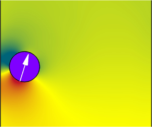
Figure 1. Schematic diagram of a circular squirmer heading downward.
In the above, the coefficient B 1 contributes to the propulsion of the squirmer, thereby determining the steady-state swimming velocity Us = B 1/2 at the Stokes flow limit. In contrast, the coefficient B 2 determines the vorticity intensity around the squirmer. Accordingly, a key parameter, defined as β = B 2/B 1, is usually introduced to represent the three types of squirmers: pushers (β < 0), pullers (β > 0) and neutral squirmers (β = 0). As indicated by the type names, pushers (e.g. bacteria such as E. coli and B. subtilis) gain thrust from their rear ends. In contrast, pullers (e.g. algae, such as C. reinhardti) gain thrust from their front ends (Koch & Subramanian Reference Koch and Subramanian2011). Neutral squirmers (e.g. Volvox) are associated with symmetric flow without vorticity (Fadda et al. Reference Fadda, Molina and Yamamoto2020). The streamline structures may provide a direct view of the propulsion mechanism for each type of squirmer, as described in § 4.2.
2.3. Boundary conditions
The improved bounce-back scheme proposed by Lallemand & Luo (Reference Lallemand and Luo2003) was used to impose no-slip boundary conditions on the surfaces of the squirmers. In their study, it was demonstrated that, based on an interpolation method, the improved bounce-back scheme shows second-order accuracy in lattice Boltzmann simulations compared with the classical bounce-back scheme with first-order accuracy (Lallemand & Luo Reference Lallemand and Luo2003). The same scheme was used in our previous studies (Nie & Lin Reference Nie and Lin2019, Reference Nie and Lin2020; Nie, Guan & Lin Reference Nie, Guan and Lin2021).
A schematic diagram for briefly introducing the scheme is shown in figure 2. As shown in the figure, the solid squares represent solid nodes located inside the solid boundary, whereas the solid circles represent the fluid nodes. The open circle denotes the boundary node where the bounce back occurs. As indicated by Lallemand & Luo (Reference Lallemand and Luo2003), a propagation action is applied to all fluid and solid nodes after the collision step. Accordingly, the distribution functions advected from solid nodes to fluid nodes must be updated depending on the exact locations of the boundary nodes; this approach differs from that of the classical scheme. To provide a better description, we consider node A as an example. As shown in figure 2, f 8 of node A is advected from a solid node (i.e. node B) during the propagation process. To update f 8, both the nearest and second nearest-neighbouring nodes along the boundary link (i.e. e8) are considered, that is, nodes B, C and D. Correspondingly, a parameter q, defined as q = |AE|/|AB|, is introduced to determine the location of the boundary node E. Then, an interpolation method can be employed to recompute f 8 according to the value of q
 \begin{align}{f_8}(\textrm{A}) = \left\{ {\begin{array}{@{}ll} {q(1 \!+\! 2q){f_6}(\textrm{B}) \!+\! (1 - 4{q^2}){f_6}(\textrm{A}) - q(1 - 2q){f_6}(\textrm{C}) + 2{w_8}\rho \dfrac{{{\boldsymbol{e}_8}\boldsymbol{\cdot }{\boldsymbol{u}_\textrm{E}}}}{{c_s^2}}}&{q < \dfrac{1}{2}}\\ {\dfrac{1}{{q(2q \!+\! 1)}}{f_6}(\textrm{B}) \!+\! \dfrac{{2q - 1}}{q}{f_8}(\textrm{C}) - \dfrac{{2q - 1}}{{2q + 1}}{f_8}(\textrm{D}) + \dfrac{{2{w_8}\rho }}{{q(2q + 1)}}\dfrac{{{\boldsymbol{e}_8}\boldsymbol{\cdot }{\boldsymbol{u}_\textrm{E}}}}{{c_s^2}}}&{q\mathrm{\ \ge }\dfrac{1}{2}} \end{array}} \right..\end{align}
Figure 2. Schematic diagram of the improved bounce-back scheme used in this work (Lallemand & Luo Reference Lallemand and Luo2003). Solid squares, solid nodes; solid circles, fluid nodes; open circles, boundary nodes.
In the above, uE is the velocity of the moving surface at boundary node E, as illustrated in figure 2. Notably, the classical bounce-back boundary is realized by (2.9) if we set q = 0.5. Further details on this scheme can be found in Lallemand & Luo (Reference Lallemand and Luo2003).
To account for the self-propelled motion of a squirmer, the velocity of the boundary node (e.g. node E) is updated by adding the slip velocity indicated in (2.8) before the interpolations, as follows:
 \begin{equation}{\boldsymbol{u}_\textrm{E}} = {\boldsymbol{u}_b} + {\boldsymbol{u}^s} = \boldsymbol{U} + \boldsymbol{\varOmega } \times \boldsymbol{R} + {\boldsymbol{u}^S}.\end{equation}
Here, U and Ω denote the translational and rotational speeds of the squirmer, respectively, and R is the position vector from the squirmer mass centre to node E. It is inferred that the self-propelled swimming of a squirmer can only be accurately resolved if there are enough boundary nodes, suggesting that squirmers with a sufficiently large diameter are needed in the simulations.
By scanning every fluid–solid boundary link, the force and torque exerted on a squirmer can be computed using a momentum exchange scheme (Mei et al. Reference Mei, Yu, Shyy and Luo2002; Lallemand & Luo Reference Lallemand and Luo2003). In addition, to account for the effects of covered or uncovered fluid nodes as a squirmer moves in a fluid, the method proposed by Aidun, Lu & Ding (Reference Aidun, Lu and Ding1998) can be used to calculate the added force and torque. Accordingly, the motion of a squirmer is determined by solving Newton's equations using the net force and torque.
2.4. Repulsive force model
When two squirmers come close to each other, a collision may occur. To address this issue, the popular repulsive model proposed by Glowinski et al. (Reference Glowinski, Pan, Hesla, Joseph and Periaux2001) was introduced, as follows:
 \begin{equation}\boldsymbol{F}_{ij}^p =
\left\{ {\begin{array}{@{}ll} 0&{\textrm{if}\ {S_{ij}} >
{R_i} + {R_j} + \xi }\\
{\dfrac{{{c_{ij}}}}{{{\varepsilon_p}}}{{\left(
{\dfrac{{{R_i} + {R_j} + \xi - {S_{ij}}}}{\xi }}
\right)}^2}\dfrac{{({\boldsymbol{X}_i} -
{\boldsymbol{X}_j})}}{{{S_{ij}}}}}&{\textrm{if}\ {S_{ij}}\le{R_i} + {R_j} + \xi } \end{array}}
\right..\end{equation}
\begin{equation}\boldsymbol{F}_{ij}^p =
\left\{ {\begin{array}{@{}ll} 0&{\textrm{if}\ {S_{ij}} >
{R_i} + {R_j} + \xi }\\
{\dfrac{{{c_{ij}}}}{{{\varepsilon_p}}}{{\left(
{\dfrac{{{R_i} + {R_j} + \xi - {S_{ij}}}}{\xi }}
\right)}^2}\dfrac{{({\boldsymbol{X}_i} -
{\boldsymbol{X}_j})}}{{{S_{ij}}}}}&{\textrm{if}\ {S_{ij}}\le{R_i} + {R_j} + \xi } \end{array}}
\right..\end{equation}
Here, Ri and Rj denote the radii of the two squirmers with mass centres at positions Xi and Xj, respectively, Sij is the distance between the mass centres, i.e.  ${S_{ij}} = |{\boldsymbol{X}_i}-{\boldsymbol{X}_j}|$, and ξ represents the cutoff distance below which the repulsive force takes effect, which was set to be 1.5Δx, where εp is a given positive stiffness parameter chosen to separate the two squirmers. As noted by Glowinski et al. (Reference Glowinski, Pan, Hesla, Joseph and Periaux2001), cij serves as a force scaling factor, and is defined as the difference between the gravitational and buoyancy forces of the squirmer in the simulations. A squirmer–wall collision is treated in a similar manner, as follows:
 \begin{equation}\boldsymbol{F}_{ij}^w =
\left\{ {\begin{array}{@{}ll}
0&{\textrm{if}\ S_{ij}^{\prime} > {R_i} + {R_j} + \xi
}\\
{\dfrac{{{c_{ij}}}}{{{\varepsilon_w}}}{{\left(
{\dfrac{{{R_i} + {R_j} + \xi - S_{ij}^{\prime}}}{\xi }}
\right)}^2}\dfrac{{({\boldsymbol{X}_i} -
\boldsymbol{X}_j^{\prime})}}{{S_{ij}^{\prime}}}}&{\textrm{if}\
S_{ij}^{\prime}\le{R_i} + {R_j} + \xi }
\end{array}} \right..\end{equation}
\begin{equation}\boldsymbol{F}_{ij}^w =
\left\{ {\begin{array}{@{}ll}
0&{\textrm{if}\ S_{ij}^{\prime} > {R_i} + {R_j} + \xi
}\\
{\dfrac{{{c_{ij}}}}{{{\varepsilon_w}}}{{\left(
{\dfrac{{{R_i} + {R_j} + \xi - S_{ij}^{\prime}}}{\xi }}
\right)}^2}\dfrac{{({\boldsymbol{X}_i} -
\boldsymbol{X}_j^{\prime})}}{{S_{ij}^{\prime}}}}&{\textrm{if}\
S_{ij}^{\prime}\le{R_i} + {R_j} + \xi }
\end{array}} \right..\end{equation}
In the above,  $\boldsymbol{X}_j^{\prime}$ is the position of the nearest imaginary squirmer's mass centre located on a wall, and accordingly, ${S^{\prime}_{ij}} = |{\boldsymbol{X}_i}-\boldsymbol{X}_j^{\prime}|$; εw is similar to εp, and is used for squirmer–wall collisions. In this study, both εp and εw were fixed at 10−3 in the simulations. This choice had little influence on the motions of the squirmers, as discussed in § 5.2.
To check the influence of collision strategy, another repulsive force model (Ishikawa et al. Reference Ishikawa, Sekiya, Imai and Yamaguchi2007; Ishikawa, Locsei & Pedley Reference Ishikawa, Locsei and Pedley2008) was also introduced, which is in exponential form as follows:
 \begin{equation}\boldsymbol{F}_{ij}^p =
\left\{ {\begin{array}{@{}ll} 0&{\textrm{if}\ {S_{ij}} >
{R_i} + {R_j} + \xi }\\
{{\alpha_1}\dfrac{{{\alpha_2}\exp [ - {\alpha_2}({S_{ij}} -
{R_i} - {R_j})/{R_i}]}}{{1 - \exp [ - {\alpha_2}({S_{ij}} -
{R_i} - {R_j})/{R_i}]}}\dfrac{{({\boldsymbol{X}_i} -
{\boldsymbol{X}_j})}}{{{S_{ij}}}}}&{\textrm{if}\
{S_{ij}}\le{R_i} + {R_j} + \xi } \end{array}}
\right.,\end{equation}
\begin{equation}\boldsymbol{F}_{ij}^p =
\left\{ {\begin{array}{@{}ll} 0&{\textrm{if}\ {S_{ij}} >
{R_i} + {R_j} + \xi }\\
{{\alpha_1}\dfrac{{{\alpha_2}\exp [ - {\alpha_2}({S_{ij}} -
{R_i} - {R_j})/{R_i}]}}{{1 - \exp [ - {\alpha_2}({S_{ij}} -
{R_i} - {R_j})/{R_i}]}}\dfrac{{({\boldsymbol{X}_i} -
{\boldsymbol{X}_j})}}{{{S_{ij}}}}}&{\textrm{if}\
{S_{ij}}\le{R_i} + {R_j} + \xi } \end{array}}
\right.,\end{equation}
where α 1 is a dimensional coefficient and α 2 is a dimensionless coefficient.
3. Problem
As illustrated in figure 3, we simulated the motion and interactions of the two squirmers under gravity in a vertical channel of a width L filled with a fluid with a density ρ and viscosity ν. The density and diameter of the squirmers are denoted by ρs and d, respectively. We use X and Y to characterize the horizontal and vertical positions, respectively. The orientation (or swimming direction) of the squirmer is denoted by ϕ. Moreover, the subscripts indexed by ‘1’ and ‘2’ are used to represent the lower (squirmer 1) and upper (squirmer 2) squirmers in the initial arrangement shown in figure 3, respectively. A moving computational domain was used to simulate an infinite channel. Doing this shifts the fluid field and squirmer positions up by one lattice spacing once the lower squirmer falls below a height of Hu from the bottom boundary. This ensures that the top boundary is always Hd away from the lower squirmer, leading to  $H = {H_u} + {H_d}$. The normal derivative of the velocity is zero at the top boundary, and the velocity at the bottom boundary is zero.

Figure 3. Schematic diagram of the problem and some notations used herein. The initial settings are as follows unless otherwise stated: X 1(0) = X 2(0) = 0, Y 1(0) = 10d, Y 2(0) = 12d, ϕ 1(0) = ϕ 2(0) = 0. The channel width is L = 5d, and the lower squirmer (squirmer 1) is initially located at a height away from the bottom boundary Hu = 10d and from the top boundary Hd = 30d. This results in a 5d × 40d computational domain.
For most of the cases studied in this work, the squirmers were initially placed at the channel centreline with a centre-to-centre distance of S (0) = 2d, as indicated in figure 3. Although the symmetrical in-line arrangement is simple, it rules out other factors to the greatest extent, suggesting that we can directly check the interactions (e.g. attraction or repulsion) between different types of squirmers. The influence of the initial arrangement is examined in § 5.2.
To account for the self-propelling strength of the squirmers in a gravitational field, a key control parameter is introduced as follows:
 \begin{equation}\alpha = \frac{{{U_s}}}{{{U_g}}}.\end{equation}
 In the above,  ${U_s} = {B_1}/2$, and Ug represents the sedimentation velocity of a non-squirmer particle settling under gravity in a channel. Notably, a Stokes-like sedimentation velocity is usually achieved for a three-dimensional study at low Reynolds numbers, based on the assumption that the gravitational and buoyancy forces are balanced by the Stokes drag for a spherical particle settling in an unbounded medium. However, there is no Stokes solution for a two-dimensional analysis. To address this issue, we adopted the analytical formula established by Happel & Brenner (Reference Happel and Brenner1965) to determine the sedimentation velocity Ug. The formula accounts for the drag of a circular cylinder of diameter d settling in a two-dimensional channel of width L at low Reynolds numbers, as follows:
 \begin{equation}{F_d} = 4{\rm \pi} K\mu {U_g}.\end{equation}
Here, μ = ρν, and K is a coefficient associated with the inverse of the blockage ratio (i.e. γ = L/d); K is defined as follows (Happel & Brenner Reference Happel and Brenner1965):
 \begin{equation}K = \frac{1}{{\ln \gamma - 0.9157 + 1.7244/{\gamma ^2} - 1.7302/{\gamma ^4} + 2.4056/{\gamma ^6} - 4.5913/{\gamma ^8}}}.\end{equation}
When the drag is balanced by the gravitational and buoyancy forces, the sedimentation velocity of a circular cylinder can be expressed as follows:
 \begin{equation}{U_g} = \frac{{{d^2}}}{{16K\mu }}({\rho _s} - \rho )g.\end{equation}
Accordingly, we can vary the value of α to adjust the strength of the self-propulsion with respect to the effect of gravity. Meanwhile, based on Ug or Us, the corresponding Reynolds number can be defined as follows:
 \begin{gather}R{e_g} = \frac{{\rho {U_g}d}}{\mu },\end{gather}
 \begin{gather}R{e_s} = \frac{{\rho {U_s}d}}{\mu }.\end{gather}
Certain parameters in the simulations were fixed as follows, unless otherwise specified: L = 5d (corresponding to γ = 5), Hu = 10d, Hd = 30d (resulting in H = 40d), ρ = 1, ρs = 1.01, d = 40 and Reg = 0.5. The initial positions of the squirmers were set as follows: X 1(0) = X 2(0) = 0, Y 1(0) = 10d and Y 2(0) = 12d. The swimming directions of both squirmers were initially downward, i.e. ϕ 1(0) = ϕ 2(0) = 0.
4. Validation
The present LBM was previously validated in our two-dimensional (Nie & Lin Reference Nie and Lin2019; Nie et al. Reference Nie, Guan and Lin2021) and three-dimensional (Nie & Lin Reference Nie and Lin2020) studies. To add credibility, the relationship for the drag of a circular cylinder (3.2) is confirmed in § 4.1. We provide a validation for the squirmer model (Blake Reference Blake1971b) in § 4.2.
4.1. Sedimentation of a non-squirmer particle in a vertical channel
Figure 4 shows the terminal velocity of a (circular) non-squirmer particle settling under gravity in a 5d channel as a function of Reg. The terminal velocity is normalized by the theoretical velocity indicated by (3.4), i.e.  $|U_T^\ast |= |{U_T}|/{U_g}$. Equation (3.4) accurately predicts the sedimentation velocity of a non-squirmer particle in a channel with a negligible fluid inertia (i.e. Reg < 1), validating the effectiveness of (3.2). Figure 4 also shows that, as Reg increases, (3.4) begins to overpredict the terminal velocity, i.e. $|U_T^\ast |< 1$. The reason for this is that the linear relationship between the drag of a particle and its velocity, as indicated by (3.2), no longer holds when the fluid inertia becomes significant.

Figure 4. Normalized terminal velocity of a non-squirmer particle (i.e.  $|U_T^\ast |= |{U_T}|/{U_g}$) settling under gravity in a 5d channel as a function of Reg. Note that $|U_T^\ast | \approx 0.99$ at Reg = 1.
4.2. Free-swimming motion of a single squirmer in an unconfined domain
To validate the squirmer model used in this study (2.8), we simulated the free-swimming motion of a single squirmer in a 20d × 20d square domain with periodic boundary conditions in all directions. Two sets of Reynolds numbers were considered: Res = 0.01 and Res = 0.5. The swimming velocity of the squirmer was normalized to Us, as shown in figure 5. As shown, the pusher is represented by β = −5, whereas the puller is represented by β = 5. It is clearly seen that the theoretical swimming velocity is achieved for each type of squirmer at Res = 0.01 (figure 5a). In addition, there is no visible difference in the time evolution of UT for all of the studied squirmers. Figure 6 (top row) shows the streamline structures around each squirmer for the same Reynolds number. The upward streamlines behind the pusher are generated by the ‘push’ action of the pusher from its rear end, as shown in figure 6 (a, top row). Accordingly, the downward swimming motion of the pusher generates downward streamlines ahead. The opposite behaviour is observed for the puller, as shown in figure 6 (c, top row). In contrast, figure 6 (b, top row) shows the streamlined structure around a neutral squirmer; it is similar to that of a non-squirmer particle. Our results agree well with those of previous studies (Ouyang et al. Reference Ouyang, Lin and Ku2018; Shen, Würger & Lintuvuori Reference Shen, Würger and Lintuvuori2018), confirming that the present computation method combined with the choice of d = 40 can accurately resolve the swimming motions of squirmers.

Figure 5. Time history of the normalized terminal velocities (UT/Us) of free-swimming squirmers in a 20d × 20d square domain with periodic boundary conditions in all directions for (a) Res = 0.01 and (b) Res = 0.5, respectively. The width of the square domain is 20d.

Figure 6. Streamlines around the squirmer at Res = 0.01 (top row) and Res = 0.5 (bottom row), respectively, for: (a) β = −5 (a pusher), (b) β = 0 (a neutral squirmer) and (c) β = 5 (a puller). Note that the arrow on each squirmer denotes its squirming axis or swimming direction (the same as below).
The situation is different at low but finite fluid inertia (e.g. Res = 0.5), as shown in figure 5(b). The pusher obtains a swimming velocity larger than  ${U_s}({U_T} \approx 1.5{U_s})$, whereas the puller obtains a smaller swimming velocity $({U_T} \approx 0.7{U_s})$. In contrast, the neutral squirmer still swims at the theoretical speed at this Reynolds number. One possible mechanism for these results is discussed in § 5.1. Note that the observations shown in figure 5(b) are qualitatively consistent with those from previous numerical studies (Lin & Gao Reference Lin and Gao2019) and theoretical predictions (Khair & Chisholm Reference Khair and Chisholm2014) for a spherical squirmer freely swimming at low but finite Reynolds numbers. The corresponding streamlines are shown in figure 6 (bottom row). It can be seen that, for both the pusher and puller, the recirculation regions upstream are suppressed whereas those downstream are stretched (owing to the higher swimming speed). However, no visible difference in the streamline structures is observed for the neutral squirmer when Res = 0.5.
5. Results
The simulation results and discussion are provided in this section. To better illustrate the interactions between two squirmers in a channel, an overview of the motion of a single squirmer settling in a channel is presented in § 5.1. The interactions between the pullers or pushers in the channel are examined in §§ 5.2 and 5.3, respectively. In particular, we describe how a puller interacts with a pusher with different initial arrangements in § 5.4. For all studied cases, the self-propelling strength factor ranges between 0.4 and 1.2, i.e. 0.4 ≤ α ≤ 1.2, and the squirmer-type factor falls within [−5, 5], i.e. −5 ≤ β ≤ 5. The results for small but non-zero α (e.g. 0 < α < 0.4) are not included in this study, because gravity nearly dominates the motions of squirmers when α is small. This is beyond our concern. However, the special case of α = 0, corresponding to the case of non-squirmer particles, is included for the purpose of comparison.
5.1. Overview of the sedimentation of a single squirmer in a channel
Figure 7 shows the instantaneous streamlines around a pusher (β = −1, −3 or −5) at a steady state at α = 1.2. The results for a non-squirmer particle are shown in figure 7(a). All cases in figure 7 exhibit a similar pattern, referred to as the ‘steady downward falling’ (SDF) pattern in this work. The most significant feature characterizing the flow around a pusher may be the ‘trailing negative flow’ behind it, as seen in figure 7(b–d). The ‘trailing negative flow’ exhibits an opposite direction as the pusher moves downward, becoming stronger and getting closer to the pusher with increasing |β|. The terminal Reynolds number (ReT) based on the terminal velocity UT is also indicated for each case in figure 8. It is clear that the UT of the pushers is more than twice that of the non-squirmer particle. In addition, the UT is larger for a pusher with a larger |β| when the self-propelling strength factor remains the same (i.e. α = 1.2); this is associated with the ‘trailing negative flow’. The stronger the ‘trailing negative flow’, the larger the reversed thrust the pusher experiences.

Figure 7. Instantaneous streamlines around a non-squirmer particle or squirmer settling in the channel, showing states of SDF for all cases: (a) α = 0 (non-squirmer), (b) β = −1 (α = 1.2), (c) β = −3 (α = 1.2) and (d) β = −5 (α = 1.2). Each result was obtained when the particle/squirmer reaches its steady state. Also shown in each panel is the terminal Reynolds number (ReT), which is based on the terminal velocity of the particle or squirmer. Note that the ‘trailing negative flow’ is seen behind the pusher, as shown in (b–d).

Figure 8. Instantaneous streamlines around a squirmer settling in the channel at α = 0.6 for (a) β = 0 (SDF), (b) β = 1 (SIF), (c) β = 3 (LSO) and (d) β = 5 (SDF). For β = 3, the result when the puller reaches its rightmost position was chosen. Note that the ‘leading negative flow’ is seen ahead of the puller for β = 5, as shown in (d).
For the settling of a single puller (β > 0), the situation is quite different. Figures 8 and 9 show the instantaneous streamlines around a puller (β = 1, 3 and 5) at α = 0.6 and 1.2, respectively. The case of a neutral squirmer is also included for comparison (figures 8a and 9a). The puller exhibits a steady state of falling downward at β = 5 for both values of α (figures 8d and 9d), similar to the behaviour of a pusher (figure 7). However, in this case, the ‘negative flow’ leads the puller. The puller gains a reversed thrust owing to the ‘leading negative flow’, resulting in a decrease in its terminal velocity (as demonstrated by the terminal Reynolds numbers indicated in figures 8a and 8d or 9a and 9d). No ‘negative flow’ is observed for the neutral squirmer (figures 8a and 9a). This also explains why the puller and pusher reach different swimming velocities at a higher Res, as shown in figure 5(b).

Figure 9. Instantaneous streamlines around a squirmer at α = 1.2 for (a) β = 0 (SDF), (b) β = 1 (SIR), (c) β = 3 (SSO) and (d) β = 5 (SDF). For β = 3, the result when the puller reaches its leftmost position was chosen. Note that the upward arrow in (b) indicates that the squirmer eventually rises (the same as below). The ‘leading negative flow’ is seen ahead of the puller for β = 5, as shown in (d).
In contrast, at β = 1, the puller ultimately reaches a steady state of inclined falling (α = 0.6, figure 8b) or inclined rising (α = 1.2, figure 9b), with its orientation upward. These patterns are referred to as ‘steady inclined falling’ (SIF) and ‘steady inclined rising’ (SIR), respectively. One possible reason for these inclined patterns is provided below. In particular, no steady state is achieved at β = 3 for the puller, which instead undergoes a periodic motion in the channel with a large scale (α = 0.6, figure 8c) or that with small scale (α = 1.2, figure 9c), designated here as ‘large-scale oscillating’ (LSO) and ‘small-scale oscillating’ (SSO) patterns, respectively. The SSO pattern was reported and referred to as the ‘attracted oscillatory mode’ in a previous study (Ouyang & Lin Reference Ouyang and Lin2022).
To better illustrate the LSO and SSO patterns, figure 10 shows the time series of the puller's horizontal position (X* = X/d) and orientation (ϕ * = ϕ/ ${\rm \pi}$) at β = 3 for α = 0.6 and α = 1.2, respectively. It is observed that for α = 0.6, the puller moves from one channel wall (X* = −2) to the other (X* = 2), with its orientation varying approximately from − ${\rm \pi}$/2 to ${\rm \pi}$/2 (figure 10a). Therefore, the pattern of the LSO is characterized by a large variation in its displacement, as well as a large variation in its orientation. In contrast, figure 10(b) shows the SSO pattern with a puller oscillating around a line close to a channel wall (i.e. X* = −2), with small amplitudes in both its displacement and orientation.

Figure 10. Time history of the horizontal position as well as the orientation of a puller (β = 3) at (a) α = 0.6 and (b) α = 1.2, illustrating the LSO and SSO patterns, respectively. Note that the horizontal position and orientation of squirmers are normalized through X* = X/d and ϕ * = ϕ/ ${\rm \pi}$ (the same as below).
It seems that pullers (β > 0) are more likely to lose their stability than pushers (β < 0) or neutral squirmers (β = 0) under the same conditions (see figures 7–9). Regarding the issue, we show the pressure contours around squirmers of different types (β = −5, 0, and 5) at α = 1.2 in figure 11. For these cases, the same state (SDF) is ultimately realized. As shown in figure 11(b), the pressure distribution of the neutral squirmer is similar to that of a non-squirmer particle (not shown here), with high-pressure and low-pressure regions observed before and behind it, respectively. For the pusher, however, significant high-pressure regions are seen both before and behind it, whereas low-pressure regions are located at both lateral sides of the pusher (figure 11a). Accordingly, the pressure distribution around the puller exhibits the opposite trend (figure 11c). Therefore, a puller may experience large repulsive forces exerted on its lateral sides as it settles downward in a channel, resulting in an unstable situation. Once the symmetrical configuration of a puller is broken, it may change into a state of SIF (figure 8b), SIR (figure 9b), LSO (figure 8c) or SSO (figure 9c). This usually occurs at a small or intermediate β value for the puller. However, at a large value of β, the wall-repulsive effects become strong, owing to the significant high-pressure regions. This suppresses the puller from deviating from the channel centreline in the presence of a flow disturbance (figures 8d and 9d). In addition, we can predict from figure 11 that two pushers attract each other when in a side-by-side arrangement, whereas two pullers repel each other. This is consistent with the findings of Götze & Gompper (Reference Götze and Gompper2010), who simulated the motion of a pair of squirmers using MPCD. To address the motion of a single puller more clearly, we conducted extensive simulations and summarized the patterns in the parametric space (α, β), as shown in figure 12.

Figure 11. Instantaneous pressure distribution around a squirmer showing the SDF pattern at α = 1.2: (a) β = −5, (b) β = 0 and (c) β = 5. Note that the pressure is normalized through  ${p^\ast } = (p - {p_\infty })/(\rho U_T^2)$, where p ∞ represents the pressure of the undisturbed flow.

Figure 12. Summarization of the patterns of motion for a puller settling in the channel in the parametric space (α, β). Each pattern of motion is characterized by one symbol (the same as below). Circle, SDF; plus, LSO; square, SSO; filled gradient, SIF; open gradient, SIR. Note that the boundaries between regions of different patterns (i.e. βc 1, βc 2 and βc 3) were obtained through the least-square scheme.
As shown in figure 12, five patterns are revealed according to both self-propelling strength (α) and squirmer type factor (β): SDF, LSO, SSO, SIF and SIR. Three boundary limits (indicated by βc 1, βc 2 and βc 3) were obtained through the least-squares scheme based on the boundary data between regions of different patterns. For β ≥ βc 1, the puller maintains its initial symmetrical configuration, and exhibits the SDF pattern of regardless of α. On the opposite side, it is widely observed that the puller loses its stability at the channel centreline before it regains it somewhere close to the channel walls when undergoing the SIF or SIR pattern, depending on both α and β.
Moreover, figure 12 shows the SSO pattern for the puller at intermediate values of β (βc 2 < β < βc 3). In particular, it is rare to find the LSO pattern for a puller, which occurs in a very narrow range of β approximately centred at βc 2, as shown in figure 12. Notably, no LSO-like pattern was reported for a puller in a 2d channel (Ouyang & Lin Reference Ouyang and Lin2022). In addition, the two oscillating patterns differ not only in their amplitudes but also in their frequencies, as shown in figure 13. This provides a comparison of the dimensionless frequency (Strouhal number, St) for the SSO and LSO patterns. It can be observed that St is much smaller for the LSO pattern than for the SSO pattern. Furthermore, the oscillating frequency exhibits opposite trends with increasing β for the two patterns (figure 13).

Figure 13. Dimensionless oscillating frequencies (Strouhal number, i.e.  $St = {f^\ast }d/{U_g}$ where f is the frequency) of a puller undergoing an LSO or SSO motion. The symbols (plus, LSO; square, SSO) are identical to those used in figure 13.
As stated above, the pusher (β < 0) maintains its initial symmetrical configuration and exhibits the SDF pattern for all values of α and β studied here in the initial downward orientation, i.e. ϕ*(0) = 0. To provide references for the study of the interactions between squirmers, we conducted extra simulations for a pusher at another initial orientation, i.e. ϕ*(0) = 0.1. The patterns are summarized in figure 14. Five similar patterns are revealed for the pushers, which are represented by the same symbols used in figure 12. Figure 14 indicates that the SDF pattern only exists at a large |β| for the pusher, similar to the case of a puller. In contrast, for almost every β falling within [−4, −2], the pusher undergoes LSO or SSO motions, depending primarily on β. However, the inclined patterns (SIF and SIR) are only observed at β = −1. Notably, the present LSO is similar to the ‘oscillatory mode’ for pushers reported by Ouyang & Lin (Reference Ouyang and Lin2022). Ahana & Thampi (Reference Ahana and Thampi2019) also revealed that weak pushers (small |β|) confined in a channel may undergo an oscillatory trajectory spanning the channel width. This type of swimming pattern can potentially be used to enhance the mixing of suspensions in microfluidic channels at low Reynolds numbers (Najafi, Raad & Yousefi Reference Najafi, Raad and Yousefi2013; Jalali, Khoshnood & Alam Reference Jalali, Khoshnood and Alam2015).

Figure 14. Summary of the pattern of a pusher's motion in the parametric space (α, β) for ϕ*(0) = 0.1. The same symbols as those in figure 13 are used, i.e. circle, SDF; plus, LSO; square, SSO; filled gradient, SIF; open gradient, SIR.
As shown in figure 14, a pusher may also form a stable inclined structure adjacent to its nearby wall, corresponding to the SIF or SIR patterns. However, a significant difference is observed between the pusher and puller, as shown in figure 15. The former has an outward orientation, whereas the latter has an inward orientation. This difference is also visible in the SSO pattern for both squirmers. To address this point, we mark all the forces experienced by each squirmer in figure 15. For the pusher, to achieve a stable structure, a self-propelling force is needed to balance the attractive force owing to the significant low-pressure regions on its left side. This requires the pusher to swim outward (figure 15a). Note that Berke et al. (Reference Berke, Turner, Berg and Lauga2008) experimentally studied the distribution of swimming bacteria (E. coli) between two glass plates and found significant attraction of the bacteria by the surfaces. From a theoretical perspective, Berke et al. (Reference Berke, Turner, Berg and Lauga2008) proposed that it is the hydrodynamic interactions with the walls that lead to the reorientation of the bacteria in the direction parallel to the walls and the attraction. This is qualitatively consistent with figure 15(a) when we consider the difference between the shapes of our pushers (circular) and the actual bacteria E. coli (spheroidal with lengths of approximately 2–3 μm and diameters of approximately 1 μm, as indicated by Koch & Subramanian Reference Koch and Subramanian2011).

Figure 15. Instantaneous contours of normalized pressure at steady state (SIF) at α = 0.6 for (a) a pusher (β = −1) and (b) a puller (β = 1). To illustrate the orientations of the squirmers, schematic diagrams of the forces experienced by each squirmer are also shown.
In contrast to the pusher, the puller needs to swim inward to ensure that its self-propelling force balances the repulsive force resulting from the high-pressure regions on its left side (figure 15b). For the swimming cells such as algae Chlamydomonas which are pullers, Berke et al. (Reference Berke, Turner, Berg and Lauga2008) predicted the attraction mechanism as well: they will simply crash into the walls. This is consistent with our observation for pullers. The low-pressure regions are located at the top and bottom of a puller (see figure 12c), so it may be attracted by nearby wall as it is reoriented in the direction perpendicular to the wall when the gravity-driven settling is not taken into account. This looks like that the puller crashes into its nearby wall.
Finally, we show the terminal velocities of squirmers of different types (β = −5, 0 and 5) as a function of α (when γ is fixed at 5) and the channel width (when α is fixed at 1.2) in figure 16. Notably, for all cases in the figure, the squirmer ultimately reaches the SDF state, except for β = 5 at γ = 8, for which the puller is seen to be steadily settling in the channel for a long time before changing to the SSO motion. To make a reasonable comparison, we adopted the steady velocity of the puller before the onset of the SSO for this case. It is clearly seen that the terminal velocity increases linearly with α (0.4 ≤ α ≤ 1.2) for all types of squirmers, with a larger growth rate for pushers and smaller rate for pullers, as shown in figure 16(a). Note that the terminal velocity of the squirmers is normalized by Ug, that is,  $|U_T^\ast |= |{U_T}|/{U_g}$. It should be stated here that for all cases considered the Reynolds numbers are so small (ReT < 2) that the flow is dominated by viscous effects. This gives rise to a linear relationship between the squirmer velocity and the driving force of squirmer. For a larger α, both the ‘trailing negative flow’ and the ‘leading negative flow’ become stronger, resulting in a larger difference in the |UT| values between a puller and pusher (figure 16a).

Figure 16. Terminal velocity of a squirmer ( $|U_T^\ast |= |{U_T}|/{U_g}$, the same as below) settling in the channel as a function of (a) α (when γ is fixed at 5) and (b) the channel width (when α is fixed at 1.2). All of the fitting curves indicated in the figure were obtained through the least-square scheme.
In contrast, the terminal velocity shows distinct trends upon varying the channel width (5 ≤ γ ≤ 8) for different squirmers, as shown in figure 16(b). This suggests different wall effects on the motions of different types of squirmers. For the pusher, |UT| monotonically increases with γ; however, for the puller, it shows a slow decreasing trend when γ > 4. In particular, it appears that the terminal velocity remains constant when γ > 4 for a neutral squirmer. This indicates that among all types of squirmers, the pullers are the most sensitive to walls when the other conditions remain the same. Similar rational formulations, i.e. (5.1a)–(5.1c), were found to fit our simulation results excellently for all squirmers (figure 16b)
 \begin{gather}|U_T^\ast |= (2.48{\gamma ^2} + 8.63\gamma + 21.66)/({\gamma ^2} + 3.16\gamma + 17.92),\end{gather}
 \begin{gather}|U_T^\ast |= (1.85{\gamma ^2} - 1.47\gamma + 11.27)/({\gamma ^2} - 1.4\gamma + 8.04),\end{gather}
 \begin{gather}|U_T^\ast |= (1.49{\gamma ^2} - 2.14\gamma + 17.42)/({\gamma ^2} - 2.46\gamma + 12.36).\end{gather}
5.2. When a puller (β > 0) meets another puller (β > 0)
In this section, we examine the interactions between two identical pullers settling under gravity in a 5d channel. Figure 17 shows the instantaneous streamlines and pressure distributions around the two settling pullers (β = 2.3) at different times for α = 1.

Figure 17. Instantaneous streamlines and pressure contours around two settling pullers at different times at β = 2.3 for α = 1: (a) t* ≈ 0.5, (b) t* ≈ 1, (c) t* ≈ 5, (d) t* ≈ 8 and (e) t* ≈ 11.
It can be seen that the pullers attract each other in the initial stage, owing to the low-pressure region between them (figures 17a and 17b). After the collision, the upper puller (referred to as ‘squirmer 2’ in figure 3) turns its orientation upward, and is driven to move toward the right wall. The lower puller (referred to as ‘squirmer 1’ in figure 3), however, remains in its downward orientation, and moves toward the other wall instead (figures 17c and 17d). Owing to their opposite orientations, the pullers quickly separate from each other (figure 17d). Our results show that the upper puller ultimately achieves the SIR state, whereas the lower puller undergoes LSO motion.
The different behaviours of the two pullers (figure 17) are not sensitive to the collision strategy ((2.11) or (2.12)). To verify this point, we performed additional simulations for the same values of α and β while choosing different stiffness parameters, i.e. εp and εw. The trajectories of the upper puller are shown in figure 18(a). There are small differences between the present computations using  ${\varepsilon _p} = {\varepsilon _w} = {10^{ - 3}}$ and those obtained using 10−5 or 10−7. However, the collision parameters do not change the patterns of the squirmers, as demonstrated in our previous studies (Nie & Lin Reference Nie and Lin2019, Reference Nie and Lin2020; Nie et al. Reference Nie, Guan and Lin2021). This is also true when the other repulsive force model (2.12) was taken into account. Note that the model (Ishikawa et al. Reference Ishikawa, Sekiya, Imai and Yamaguchi2007, Reference Ishikawa, Locsei and Pedley2008) is in exponential form, completely different from the algebraic one we adopted here (Glowinski et al. Reference Glowinski, Pan, Hesla, Joseph and Periaux2001). In addition, we checked the influence of the initial arrangements by varying the initial position of the upper puller while keeping that of the lower one unchanged. Selected results are shown in figure 18(b), and show the same solution (SIR) as that obtained from the initial arrangement indicated in figure 3 or its symmetrical counterpart, despite the fact that the upper puller was released from various positions. Correspondingly, the lower puller undergoes an LSO motion for all settings, as indicated in figure 18(b). Therefore, the patterns revealed here are applicable to various initial configurations.

Figure 18. Effects of (a) collision parameter and (b) initial arrangement on the trajectory of the upper puller (i.e. squirmer 2 shown in figure 3). The repulsive force model (2.12) which is in exponential form was also checked in (a). The same α and β as those in figure 17 were chosen. The small circles represent the initial positions of the upper puller. Note that the initial position of the lower puller (referred to as ‘squirmer 1’ in figure 3) remains unchanged for all cases studied.
Our results indicate that both pullers are likely to gain a stable structure adjacent to their nearby channel walls (i.e. SIF or SIR) after they interact or collide with each other, especially at a large α. Figure 19 shows the instantaneous streamlines around two settling squirmers at steady states at different values of β for α = 1, i.e. the same α as in figure 17. β = 0 corresponds to neutral squirmers. Both figures 17 and 19 suggest that the pullers may change their orientations noticeably when they come to contact, qualitatively in accord with previous studies (Ishikawa et al. Reference Ishikawa, Simmonds and Pedley2006, Reference Ishikawa, Sekiya, Imai and Yamaguchi2007). The SIF pattern is seen for both squirmers at small values of β (figures 19a and 19b), whereas the SIR is seen at large values of β (figures 19c and 19d). In addition, squirmers are more inclined with respect to the channel walls at larger values of β. The reason is explained as follows. The larger the value of β , the more significant the high-pressure regions on the lateral sides of a puller (see figure 11c). As a result, the pullers need to be more inclined to attain a larger horizontal component of the self-propelling force to achieve a stable structure (see figure 15b). In particular, neutral squirmers showed no visible inclination when they reach a steady state in the channel (figure 19a). This is reasonable, because there are no significant low-pressure or high-pressure regions on the lateral sides of a neutral squirmer, unlike in the case of a puller or pusher (see figure 11). As a result, there is no need for a neutral squirmer to incline its swimming direction to attain a stable configuration. Figure 19 also indicates that the squirmers come closer to their nearby walls at a larger β. The primary reason for this is provided below. For a puller, low-pressure regions can be seen at its front (figure 11c); these turn into an attractive force when the puller is inclined to its nearby wall (see also figure 15b). The attractive force becomes stronger at a larger β, causing the puller to move closer to the wall.

Figure 19. Instantaneous streamlines around two settling squirmers at steady state for α = 1: (a) β = 0 (neutral), (b) β = 1, (c) β = 3 and (d) β = 5.
To provide greater insight into the interactions between squirmers (β ≥ 0), we performed a large number of simulations. The patterns of the lower and upper squirmers are summarized in figures 20(a) and 20(b), respectively. The same symbols as those used in figure 12 are adopted except for the symbol of the cross (X), a new symbol used to represent a new pattern for which the squirmers interact with each other all the time and oscillate in the channel. Note that the oscillations are non-periodic. This new pattern is beyond the scope of this paper. It is clearly seen from figure 20 that the squirmers (β ≥ 0) settle separately in the channel while exhibiting the same or different patterns for all α and β values considered, except for those indicated by X (small β at 0.4 ≤ α ≤ 0.9). This is significantly different from the situation in which two non-squirmer particles settle under gravity in a channel at similar Reynolds numbers. Previous studies (Feng, Hu & Joseph Reference Feng, Hu and Joseph1994; Nie & Lin Reference Nie and Lin2019) have indicated that non-squirmer particles may form a stable staggered configuration in which they rotate in the same direction at Re ∼ O(1). Further increasing the Reynolds number may lead to a periodic motion of particles or drafting–kissing–tumbling (DKT) interactions between the particles (Feng et al. Reference Feng, Hu and Joseph1994). Notably, no DKT motions are observed for any of the cases considered here.

Figure 20. Summary of the patterns of two interacting squirmers (β ≥ 0) in the channel in the parametric space (α, β): (a) lower squirmer (squirmer 1) and (b) upper squirmer (squirmer 2). Note that all the symbols (plus, LSO; square, SSO; filled gradient, SIF; open gradient, SIR) are identical to those in figure 12 except for a new one, i.e. the symbol of the cross ‘X’, which was used here to represent a pattern of squirmers oscillating.
The interactions between pullers have significant influences on the motion of both pullers as compared with figure 12 (showing the patterns of a single one). Interestingly, there is no SDF pattern for either puller (figure 20). This is primarily because the pullers always attract each other once they are released and eventually collide with each other (see also figure 17). Then, both pullers, which are initially moving downward, change their orientations, leading to patterns other than SDF. The close contact of the pullers changes their respective orientations in different manners, with the upper one always facing upward, whereas the lower one may remain downward or face upward depending on β at a certain α (figure 20). Consequently, the upper puller is always attracted by its nearby wall and reaches a steady inclined state (SIF or SIR), as shown in figure 20(b). The boundary between the SIF and SIR regions can be approximately formulated by a linear function related to a critical β, i.e. βc 4(α), as indicated in figure 20(b) (with its value decreasing with α). In contrast, it is the lower puller exhibits the LSO pattern for a narrow range of β; this can still be accounted for by the same formulation βc 2(α), as indicated in figure 12. However, the SSO pattern only exists at β values slightly larger than βc 2, which differs from figure 12, suggesting that the pullers are highly likely to lose stability and give rise to oscillating motions at intermediate values of β. In general, an inclined state (SIF or SIR) is largely observed for the lower puller, owing to its interactions with the upper puller.
5.3. When a pusher (β < 0) meets another pusher (β < 0)
Compared with the case for pullers, the interactions between two pushers are much simpler, and are in accordance with the observation of a single squirmer as discussed in § 5.1. In general, only the SDF pattern is observed for the pushers. Figure 21 shows the instantaneous streamlines and pressure contours around two pushers (β = −3) at different times for α = 1.2. The pushers repel each other once they are released in the channel owing to the high-pressure regions between them (figure 21a,b), which is contrary to the case with the pullers (figure 17). As the upper pusher moves farther away, the ‘trailing negative flow’ behind the lower pusher becomes more significant (figure 21c,d), further driving the pushers apart from each other. Figure 22 shows the instantaneous streamlines around two pushers with different β values at t* ≈ 100. Figure 22(a,b) suggests that the ‘trailing negative flow’ is not the basic reason for the repulsion of the pushers. At small values of |β|, no visible ‘negative flow’ is seen behind the lower pusher; it becomes visible at larger values of |β| and helps to accelerate the separation of the pushers, as indicated in figure 22(c,d).

Figure 21. Instantaneous streamlines and pressure distributions around two settling pushers (β = −3) for α = 1.2 at different times: (a) t* ≈ 1, (b) t* ≈ 10, (c) t* ≈ 40 and (d) t* ≈ 100.

Figure 22. Instantaneous streamlines around settling pushers at t* ≈ 100 for α = 1.2: (a) β = −1, (b) β = −2, (c) β = −4 and (d) β = −5.
Our simulations show that the pushers move farther away from each other over time. In other words, the pushers will never come close to each other, owing to the high-pressure regions between them (figure 21). To address this point, we present the time history of the distances between the pushers at different values of β for both α = 0.6 and 1.2 in figure 23. The distance is normalized by d, i.e. S* = S/d. It is clearly seen that S* increases monotonically with time for all cases considered. In particular, a similar slope is obtained at t* > 10 at a large |β| (e.g. |β| ≥ 3) for either α.

Figure 23. Time history of the normalized distances (S* = S/d) between pushers at different β for (a) α = 0.6 and (b) α = 1.2.
5.4. When a puller (β > 0) meets a pusher (β < 0)
In this section, we examine the interactions between the puller and pusher. We only consider two situations: a pusher initially placed above a puller, and its opposite. For simplicity, the squirmers are assumed to have the same value of |β|. Figure 16 indicates that a pusher always moves faster in a channel than a puller if it has the same value of |β|. Accordingly, for the former situation, it is commonly observed that the pusher (say β = −5) approaches the puller (say β = 5) once they are released from rest, and ultimately, a stable doublet is formed, as shown in figure 24. For comparison, the case of non-squirmer particles is also shown in figure 24(a).

Figure 24. Instantaneous streamlines around settling doublets at steady state: (a) α = 0 (non-squirmer), (b) α = 0.4, (c) α = 0.6, (d) α = 0.8 and (e) α = 1. Note that the doublet consists of a pusher (β = −5, upper) and a puller (β = 5, lower) for α > 0 (the same as below).
Our results also indicate that the doublets remain stable for a very long time (t* > 500) before the computations are terminated. They may collapse at the end, but this was not observed. In addition, the doublet formed by squirmers moves much faster than one formed by non-squirmer particles. For instance, the terminal velocity of the doublet for α = 0.8 is more than twice that for α = 0 (non-squirmer particle).
Another significant feature in the flow around a doublet concerns the absence of the ‘leading negative flow’ before the puller (figure 24b–e). The ‘trailing negative flow’, however, is visible behind the doublet for all values of α (α > 0). To address this issue, we show the instantaneous streamlines and contours of the vertical fluid velocity (normalized by Ug, i.e.  ${v^\ast } = v/{U_g}$) during the initial stage at α = 1.2 in figure 25. In fact, the ‘leading negative flow’ is visible before the doublet at t* ≤ 0.2, whose intensity decays quickly, as reflected by the magnitude of the vertical fluid velocity (figure 25a–c). At t* ≈ 0.3, the ‘leading negative flow’ completely disappears as the doublet is finally formed (figure 25d). The reason is simple. The settling velocity of the puller increases as the pusher comes closer to it, driving the ‘leading negative flow’ farther away from the puller, as shown in figure 25(a–c). As the doublet is formed, the puller attains a much larger velocity than that of itself without the presence of a pusher (see figures 8d and 24c). In addition, the resulting accelerated doublet also drives the ‘trailing negative flow’ farther behind, whose intensity is significantly reduced (figure 25d).

Figure 25. Instantaneous streamlines around two settling squirmers (upper pusher: β = −5, lower puller: β = 5) and contours of the vertical fluid velocity during the initial stage for α = 1.2: (a) t* ≈ 0.03, (b) t* ≈ 0.08, (c) t* ≈ 0.2 and (d) t* ≈ 0.3. Note that the vertical velocity of fluid is normalized through  ${v^\ast } = v/{U_g}$.
When a puller is initially above a pusher (corresponding to the second situation), the squirmers are always observed to separate from each other at the initial stage, because a pusher moves faster than a puller at the same |β|. It was shown in § 5.1 that a pusher always achieves a steady state (i.e. SDF) at the channel centreline if it is initially facing downward. However, this may not be the case if a puller is trailing. As shown in figure 12, a puller is very likely to lose its initial symmetrical configuration and subsequently exhibit different patterns; this may alter the steady state of a pusher below, owing to their interactions. To provide a quantitative analysis, we summarized the patterns of interacting squirmers for the second situation, and show them separately in figure 26. It can be seen that the pusher achieves the SDF pattern only at large values of |β| (figure 26a), because the puller above settles steadily along the channel centreline at the same |β| (figure 26b). Except for the SDF pattern, the pusher is largely seen to undergo an oscillating motion (LSO or SSO) at intermediate |β| values, or to reach an inclined state (SIF or SIR) at small |β| values (figure 26a). These results are very similar to those of figure 14, which shows the patterns of a pusher with non-zero initial orientations. In contrast, the puller always exhibits an SIF or SIR pattern at these values of |β| (figure 26b). In particular, the effects of interactions on the motion of the puller are clearly indicated by the results marked with a grey background in figure 26(b); these are designated as the LSO or the SSO in figure 12, which summarizes the patterns of a single puller in the same channel. However, the interactions between the squirmers show no influence on the motion of the pusher, in contrast to figure 14. For additional details, we present the results for interacting squirmers (a puller with β = 3 and pusher with β = −3) at α = 0.8 in figures 27 and 28.

Figure 26. Summary of the patterns of interacting squirmers in the parametric space (α, β) for the situation where a puller is initially placed above a pusher: (a) the pusher and (b) the puller. As a reminder, each pattern represented by one symbol is reiterated as follows. Circle, SDF; square, SSO; plus, LSO; filled gradient, SIF; open gradient, SIR.

Figure 27. Time history of the positions of the pusher (β = −3) and the puller (β = 3) at α = 0.8: (a) horizontal component and (b) vertical component.

Figure 28. Instantaneous streamlines around the settling squirmers at α = 0.8 at different times showing the interactions between a pusher (β = −3) and puller (β = 3): (a) t* ≈ 10, (b) t* ≈ 40, (c) t* ≈ 130, (d) t* ≈ 150 and (e) t* ≈ 160.
Figure 27 shows the time histories of the horizontal and vertical positions of the squirmers at t* ≤ 180. The instantaneous streamlines around the squirmers at the representative times are illustrated in figure 28. It is clear that the pusher loses its stability at t* ≈ 30, the same time at which the puller departs from the channel centreline, as indicated by their horizontal positions in figure 27(a). Subsequently, the puller quickly changes to an oscillating motion (SSO) near the left wall (figure 28b). In contrast, it takes a much longer time (t* > 115) for the pusher to finally realize a LSO motion (figure 27a). Figure 28(c) shows the corresponding streamlines. Before t* = 115, the distance between the squirmers increases with time as the pusher attains a larger settling velocity, as indicated in figure 27(b).
The onset of the LSO motion leads to a significant drop in the settling velocity of the pusher, leading to the fact that the puller settles faster than the pusher. This is confirmed by figure 27(b), which shows a decreasing trend in the distance between the squirmers at t* > 115. The puller finally approaches the pusher at t* ≈ 150 (figures 27b and 28d). After contact, the puller turns its orientation upward and ultimately reaches a steady state (SIR) near the right wall (i.e. X* = 2) instead of oscillating. In contrast, the pusher retains its oscillating motion (LSO) in the channel (figures 27a and 28e). Because the puller has an upward orientation while the pusher remains downward, the two squirmers begin to separate once again (t* > 150), as indicated by figure 27(b).
6. Summary
We conducted a numerical study on the motions and interactions of squirmers in a vertical channel using two-dimensional lattice Boltzmann simulations. In addition to the squirmer-type factor (β), another control parameter, namely the self-propelling strength factor, was introduced as α = Us/Ug. In this calculation, Us denotes the steady swimming velocity of a squirmer, and Ug represents the gravity-driven settling velocity of a non-squirmer particle with the same diameter in a channel in the Stokes flow regime. To better understand the interactions of the squirmers, we first considered the motion of a single squirmer under gravity in a 5d (d is the diameter of the squirmers) channel at 0.4 ≤ α ≤ 1.2 and −5 ≤ β ≤ 5. Based on this, the interactions between two pullers (β > 0) and two pushers (β < 0) in the same channel were successively investigated. Finally, we considered the interactions between the pusher and puller. The summary of this study is provided below.
(i) Results show that a single puller reaches a steady state (SDF) along the channel centreline at a large β (β ≥ βc 1 where βc 1 is a critical β). At β < βc 1, the puller is likely to lose its stability and symmetrical structure, owing to the high-pressure regions on both lateral sides. Accordingly, an LSO motion is eventually achieved for the puller when β is close to another critical value, that is, β ≈ βc 2. In contrast, it is observed that the puller undergoes an SSO motion at βc 2 < β ≤ βc 3, where βc 3 denotes the third critical value of β. Otherwise, the puller achieves an inclined state adjacent to its nearby wall, that is, the SIF or SIR pattern, depending on both α and β. Notably, all of these critical β values (βc 1, βc 2 and βc 3) are dependent on α. In particular, an LSO motion rarely occurs for a puller, which differs from an SSO motion in terms of the amplitudes in both the position and orientation of the puller.
The situation is much simpler for a pusher or neutral squirmer, which always reaches a steady state (SDF) when initially facing downward (i.e. at zero initial orientation). A pusher may undergo an oscillating motion (LSO or SSO) or achieve an inclined state (SIF or SIR) at non-zero initial orientations. However, for the inclined patterns, a distinct difference is found between different squirmers, with a puller facing toward its nearby wall and a pusher facing outward from its nearby wall. This is primarily caused by the different pressure distributions around the different squirmers.
For the SDF pattern, the terminal velocity of a single squirmer increases linearly with α for all types of squirmers. For a fixed α, the pusher always moves faster than the puller, whereas the neutral squirmer is in between. The primary reason is associated with the ‘leading negative flow’ before a puller and ‘trailing negative flow’ behind a pusher, which become more significant at larger values of β. A puller experiences a reversed thrust from the ‘leading negative flow’ as it falls, resulting in a decrease in its settling velocity. However, the ‘trailing negative flow’ does the opposite to a pusher. There is no ‘negative flow’ for a neutral squirmer. Different types of squirmers show different trends in their terminal velocities with increasing channel width.
(ii) The interactions between two pullers are complex. The SDF pattern observed for a single puller at a large β does not exist in this situation. For most cases of two squirmers (−5 ≤ β ≤ 5) released in a channel, they may interact with each other for a certain time, but in the end, they settle in the channel separately while exhibiting the same or different patterns of motion. In general, our simulations show that both pullers begin to attract each other once they are released from rest, owing to the low-pressure regions between them. They may quickly come into contact. After that, the upper puller attains an upward orientation and reaches an inclined state (SIF or SIR, respectively). However, the lower puller undergoes an LSO motion at β ≈ βc 2, similar to the case of a single puller. In particular, the SSO motion occurs only at some values of β that are slightly larger than βc 2. Otherwise, the lower puller exhibits an SIF or SIR pattern.
(iii) In comparison with pullers, the interactions between two pushers are simple. Only the SDF pattern is observed for both pushers in all studied cases. Pushers always repel each other and begin to separate once they are released, owing to the high-pressure regions between them. In addition, the ‘trailing negative flow’ behind the lower pusher, which becomes strong at larger values of β, is seen to further increase the separation between the pushers.
(iv) Regarding the interactions between a puller and pusher, two situations were considered: a pusher initially leading a puller and its opposite. For both cases, we assumed that both squirmers had the same |β|. In the former situation, the pusher always approaches the puller, because the pusher moves faster than a puller at the same |β|. Then, a stable doublet is quickly formed, and shows a noticeably large settling velocity compared with the case of non-squirmer particles or a single squirmer. In contrast, the latter situation is quite different. Both squirmers separate at the initial stage. However, apart from the SDF pattern at large |β| values observed for a single pusher at all values of |β|, the pusher may exhibit an oscillating motion (LSO or SSO) at an intermediate |β| or an inclined state (SIF or SIR) at a small |β|, as a result of its interactions with the puller. The most significant effect of the interactions on the puller is that there is no oscillating motion (LSO or SSO) for it, as compared with the case of a single puller undergoing the LSO or SSO motion at intermediate values of |β|. The reason for this is briefly explained below. The puller quickly turns into an oscillating motion as it separates from the pusher. The pusher loses stability and requires a long time to realize an oscillating motion. This significantly reduces the settling velocity. Subsequently, the puller approaches it. After contact, the puller turns its orientation upward, and ultimately reaches a steady state adjacent to its nearby wall. However, the contact does not change the orientation of the pusher. In other words, it remains downward, and continues to oscillate.
(v) It should be more interesting to perform three-dimensional analysis of squirmers settling under gravity in a tube. In addition to the patterns exhibited by circular squirmers, the extra dimension may allow different dynamical features to occur for spherical squirmers (e.g. the spiral or zigzagging trajectory). On the other hand, the gravity-driven motion of interacting squirmers at moderate Reynolds numbers where the fluid inertia play an important role deserves more efforts. This becomes our future work.
Funding
This study was supported by the National Natural Science Foundation of China (nos 12132015 and 11972336).
Declaration of interests
The authors report no conflict of interest.


