


1. Introduction
Information about bathymetry, or the topography of the seafloor, is critical for a wide range of applications, such as the safety of navigation, accuracy of ocean wave models, habitat mapping and hydrographic charting (Matsuyama, Walsh & Yeh Reference Matsuyama, Walsh and Yeh1999; Wilson et al. Reference Wilson, O'Connell, Brown, Guinan and Grehan2007; Holman & Haller Reference Holman and Haller2013; Wölfl et al. Reference Wölfl2019; Monteiro et al. Reference Monteiro, Jiménez, Gizzi, Přikryl, Lefcheck, Santos and Canning-Clode2021). To obtain bathymetric data, there are several direct measurement techniques using acoustic devices, satellite-derived bathymetry (SDB) and bathymetric light detection and ranging (LiDAR). Acoustic devices such as echo-sounders emit and receive acoustic signals, and the depths of the seafloor are estimated by measuring the two-way travel time of a sound wave transmitted to and back from the seafloor (De Moustier Reference De Moustier1986). In another seafloor mapping technique, SDB, satellite platforms obtain multispectral satellite imagery covering the visible to infrared portions of the spectrum. The attenuation of the electromagnetic signal in the water column as a function of the wavelength is used to calculate the water depth (Cahalane et al. Reference Cahalane, Magee, Monteys, Casal, Hanafin and Harris2019). The use of SDB is limited by environmental conditions such as cloud cover and water turbidity. Bathymetric LiDAR, a technology that sends laser pulses from an airborne platform and records their return, is another method for mapping bathymetry data. The time difference between the reflection from the water surface and that from the seafloor is used to calculate the water depth (Irish & White Reference Irish and White1998). However, such optical solutions can be obtained only in shallow waters with good water clarity.
In contrast to the direct measurement techniques reviewed above, which are expensive and limited by environmental conditions, there have been studies to invert bathymetry by combining surface wave information, which can be measured using modern wave gauging and mapping techniques, with wave dynamics. In early years, the methods to invert bathymetry from surface waves were based on the dependence of the linear dispersion relation of surface waves on the depth (e.g. Lubard et al. Reference Lubard, Krimmel, Thebaud, Evans and Shemdin1980; Grilli Reference Grilli1998; Trizna Reference Trizna2001; Piotrowski & Dugan Reference Piotrowski and Dugan2002). In addition to the methods solely relying on the dispersion relation, Nicholls & Taber (Reference Nicholls and Taber2009) derived explicit formulae to obtain bathymetry data from the free-surface data using a Dirichlet to Neumann operator. However, their method is only focused on standing waves, which are uncommon in oceans. Vasan & Deconinck (Reference Vasan and Deconinck2013) presented a method based on the Euler equations that can be applied to transient free-surface data. However, the computational cost, which is related to the number of Fourier modes, is non-trivial for recovering two-dimensional bathymetry. Vasan et al. (Reference Vasan, Manisha and Auroux2021) introduced an algorithm for estimating the ocean bottom using shallow-water wave equations by assuming a relatively inaccurate initial bottom guess. Khan & Kevlahan (Reference Khan and Kevlahan2021) proposed a method based on variational data assimilation for a one-dimensional shallow water equation by assuming that the wavelength is much larger than the water depth. These wave physics-based methodologies mainly focus on relatively simple conditions where the bathymetry exhibits one-dimensional variation, the surface waves are assumed to be periodic and narrow-banded, and the effect of measurement noise is neglected.
Nearshore surface wave modelling has been studied extensively in the past several decades. The methods can be divided into two main categories. The first category of methods is based on the long-wave approximation, such as the Boussinesq or shallow water equations, by assuming that the wavelength is much larger than the water depth (Peregrine Reference Peregrine1966; Grimshaw Reference Grimshaw1970; Wei et al. Reference Wei, Kirby, Grilli and Subramanya1995; Madsen, Bingham & Liu Reference Madsen, Bingham and Liu2002; Feddersen Reference Feddersen2014). The second category of methods relies on computing power advancement to enable solution of the full Euler equations, including methods that solve nonlinear potential flow-based equations with a free surface using the boundary integral method (Clamond & Grue Reference Clamond and Grue2001; Grilli, Guyenne & Dias Reference Grilli, Guyenne and Dias2001; Wilkening & Vasan Reference Wilkening and Vasan2015) and methods that utilise spectral methods based on nonlinear perturbation expansions to perform nonlinear wave simulations for infinite or constant depth (Dommermuth & Yue Reference Dommermuth and Yue1987; West et al. Reference West, Brueckner, Janda, Milder and Milton1987; Craig & Sulem Reference Craig and Sulem1993; Nicholls Reference Nicholls1998) and extensions to variable bottoms (Liu & Yue Reference Liu and Yue1998; Smith Reference Smith1998; Guyenne & Nicholls Reference Guyenne and Nicholls2008). These methods have a wide range of applications, such as nonlinear wave shoaling, Bragg scattering and tsunami generation (Liu & Yue Reference Liu and Yue1998; Guyenne & Nicholls Reference Guyenne and Nicholls2008; Alam, Liu & Yue Reference Alam, Liu and Yue2009a,Reference Alam, Liu and Yueb; Gouin, Ducrozet & Ferrant Reference Gouin, Ducrozet and Ferrant2016; Hao & Shen Reference Hao and Shen2022).
As a powerful tool, adjoint-based data assimilation methods aim to find the optimal control variables that minimise a predefined cost function used to quantify the difference between measurement data and model prediction. Gradient-based optimisation approaches are often employed to solve constrained optimisation problems in data assimilation. Compared with stochastic methods (Cavazzuti Reference Cavazzuti2012), gradient-based optimisation techniques require fewer iterations to reach convergence, resulting in a lower computational cost for complex systems. For instance, the limited-memory Broyden–Fletcher–Goldfarb–Shanno (L-BFGS) method (Byrd et al. Reference Byrd, Lu, Nocedal and Zhu1995; Zhu et al. Reference Zhu, Byrd, Lu and Nocedal1997) has been widely used because the memory requirement is affordable even when the dimension of the Hessian matrix is high, e.g.  $O(10^9)$. The gradients of the cost function with respect to the control parameters are used to identify the search direction for minimising the cost function. In a complex system with high degrees of freedom, however, calculating the gradients directly is computationally expensive. To solve this problem, the adjoint method is employed with the key benefit that the computational cost of gradient calculation is independent of the degrees of freedom of the control variables (Gronskis, Heitz & Mémin Reference Gronskis, Heitz and Mémin2013; Foures et al. Reference Foures, Dovetta, Sipp and Schmid2014; Wu, Hao & Shen Reference Wu, Hao and Shen2022).
In this study, we propose a bathymetry reconstruction method that can be applied to realistic coastal environments involving complex two-dimensional bathymetry features, non-periodic incident waves and nonlinear broadband multidirectional waves. We also address issues related to the surface wave data quality, including limited sampling frequency and noise. Our method combines the high-order spectral (HOS) method for finite-depth waves developed by Liu & Yue (Reference Liu and Yue1998) to capture the nonlinear wave evolution over complex bathymetry and the adjoint-based data assimilation method that is widely used in fields such as meteorology, oceanography, fluid dynamics and climate modelling (Errico Reference Errico1997; Moore et al. Reference Moore, Arango, Di Lorenzo, Cornuelle, Miller and Neilson2004; Foures et al. Reference Foures, Dovetta, Sipp and Schmid2014; Xu & Wei Reference Xu and Wei2016). Note that Khan & Kevlahan (Reference Khan and Kevlahan2021, Reference Khan and Kevlahan2022) adopted the variational data assimilation approach using the shallow-water wave equation to reconstruct bathymetry from a limited subset of surface elevation measurements. Their work primarily focused on bathymetry detection from sparse measurements of surface elevation. In contrast, our work focuses on precise bathymetry detection from dense surface measurements, such as from marine radars in realistic coastal environments. Additionally, deriving an adjoint model for the HOS model for arbitrarily high perturbation orders is a non-trivial task. Previous studies on the adjoint method for the HOS model have been limited to the third perturbation order and relied on expanding the water wave equations to the specific perturbation order and then deriving adjoint terms accordingly (Aragh & Nwogu Reference Aragh and Nwogu2008; Wu et al. Reference Wu, Hao and Shen2022). However, the number of terms in the wave equations increases rapidly with the perturbation order, making it infeasible for higher perturbation orders. Nonetheless, high perturbation orders are necessary for accurately capturing bottom–wave interaction using the HOS method. Our recursive adjoint model overcomes the limitations of previous work and enables the use of adjoint-based HOS methods effectively for the task of bathymetry reconstruction.
The remainder of this paper is organised as follows. The proposed bathymetry inversion algorithm is first introduced in § 2. Test cases for laboratory-scale and field-scale bathymetry reconstruction under monochromatic and broadband waves are then presented in § 3. The effects of the measurement sampling frequency and measurement noise are studied in § 4. The effects of small bottom variations and limited measurements are discussed in § 5. Finally, discussion and conclusions are provided in § 6.
2. Bathymetry inversion method using adjoint-based data assimilation
2.1. Nonlinear wave simulation over variable bathymetry
We employ the HOS method (Dommermuth & Yue Reference Dommermuth and Yue1987; West et al. Reference West, Brueckner, Janda, Milder and Milton1987; Liu & Yue Reference Liu and Yue1998; Alam et al. Reference Alam, Liu and Yue2009a,Reference Alam, Liu and Yueb) to simulate nonlinear wave propagation over bathymetry by assuming that the flow is inviscid, irrotational and incompressible. Thus, the flow velocity can be expressed using the velocity potential function  $\varPhi (x,y,z,t)$ which satisfies the Laplace equation inside the fluid domain and the boundary conditions at the free surface $z=\eta (x,y,t)$ and bottom $z=-h+\beta (x,y)$, where $h$ is a constant reference depth and $\beta (x,y)$ denotes the bottom spatial variation. The governing equations and boundary conditions are
 $$\begin{gather} \nabla^2\varPhi +\varPhi_{zz}= 0 \quad \text{for} \ -h+\beta(x,y)< z<\eta(x,y,t), \end{gather}$$
 $$\begin{gather}\varPhi_z-\boldsymbol{\nabla}\beta \boldsymbol{\cdot} \boldsymbol{\nabla}\varPhi=0 \quad \text{on} \ z={-}h+\beta(x,y), \end{gather}$$
 $$\begin{gather}\eta_{t}+\boldsymbol{\nabla}\eta\boldsymbol{\cdot}\boldsymbol{\nabla}\varPhi-\varPhi_z=0 \quad \text{on}\ z=\eta(x,y,t), \end{gather}$$
 $$\begin{gather}\varPhi_t+g\eta+\tfrac{1}{2}(\boldsymbol{\nabla}\varPhi\boldsymbol{\cdot}\boldsymbol{\nabla}\varPhi+\varPhi_z^2)=0 \quad \text{on} \ z=\eta(x,y,t), \end{gather}$$
where  $x$ and $y$ denote the horizontal coordinates, $z$ denotes the vertical coordinate, $\boldsymbol {\nabla }=(\partial /\partial x, \partial / \partial y)$ is the gradient operator in the horizontal directions, the subscripts in $\varPhi _z$ and $\varPhi _{zz}$ denote the first-order and second-order partial derivatives in the $z$-coordinate, respectively, and $g$ represents gravitational acceleration.
As pointed out in Liu & Yue (Reference Liu and Yue1998), assuming both bottom and free-surface slopes are measured by the same small quantity  $\epsilon \ll 1$, we can write the velocity potential, surface elevation and bottom profile in perturbation series as
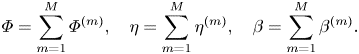 \begin{equation} \varPhi = \sum_{m=1}^M\varPhi^{(m)}, \quad \eta=\sum_{m=1}^M\eta^{(m)}, \quad \beta=\sum_{m=1}^M\beta^{(m)}. \end{equation}
In the equation above,  $()^{(m)}$ is a quantity of magnitude $O(\epsilon ^m)$; $\varPhi ^{(m)}$ satisfies the Laplace equation within the fluid; $M$ is the nonlinear perturbation order. Through the Taylor expansion, we can obtain the vertical velocity at the free surface expressed by the surface velocity potential $\varPhi ^s(x,y,t)\equiv \varPhi (x,y,z=\eta,t)$ and surface elevation $\eta (x,y,t)$ as (Dommermuth & Yue Reference Dommermuth and Yue1987; West et al. Reference West, Brueckner, Janda, Milder and Milton1987; Liu & Yue Reference Liu and Yue1998; Alam et al. Reference Alam, Liu and Yue2009a,Reference Alam, Liu and Yueb)
 $$\begin{gather} \varPhi^{(1)}(x,0,t) = \varPhi^s, \end{gather}$$
 $$\begin{gather}\varPhi^{(m)}(x,0,t) ={-}\sum_{l=1}^{m-1}\frac{\eta^l}{l!}\frac{\partial ^l}{\partial z^l}\varPhi^{(m-l)}(x,0,t), \quad m=2,3,\ldots,M, \end{gather}$$
 $$\begin{gather}\varPhi_z^{(1)}(x,-h,t) = 0, \end{gather}$$
 $$\begin{gather}\varPhi_z^{(m)}(x,-h,t) = \sum_{l=1}^{m-1}\boldsymbol{\nabla}\boldsymbol{\cdot}\left(\frac{\beta^l}{l!}\frac{\partial^{l-1}}{\partial z^{l-1}}\boldsymbol{\nabla }\varPhi^{(m-l)}(x,-h,t)\right), \quad m=2,3,\ldots,M. \end{gather}$$
 By employing the HOS method, one can use only the free-surface elevation  $\eta$ and surface velocity potential $\varPhi ^s$ to evolve the wave field. The time evolution of $\eta$ and $\varPhi ^s$ can be written as (Dommermuth & Yue Reference Dommermuth and Yue1987; West et al. Reference West, Brueckner, Janda, Milder and Milton1987; Liu & Yue Reference Liu and Yue1998; Alam et al. Reference Alam, Liu and Yue2009a,Reference Alam, Liu and Yueb)
 $$\begin{gather} \eta_t+\boldsymbol{\nabla} \varPhi^s\boldsymbol{\cdot}\boldsymbol{\nabla}\eta=(1+\boldsymbol{\nabla}\eta\boldsymbol{\cdot}\boldsymbol{\nabla}\eta)W, \end{gather}$$
 $$\begin{gather}\varPhi^s_t+\tfrac{1}{2}\boldsymbol{\nabla}\varPhi^s\boldsymbol{\cdot}\boldsymbol{\nabla}\varPhi^s+g\eta=\tfrac{1}{2}(1+\boldsymbol{\nabla}\eta\boldsymbol{\cdot}\boldsymbol{\nabla}\eta)W^2, \end{gather}$$
 $$\begin{gather}W=\sum_{m=1}^{M}\sum_{l=0}^{M-m}\frac{\eta^l}{l!}\frac{\partial ^{l+1}}{\partial z^{l+1}}\varPhi^{(m)}(x,0,t), \end{gather}$$
where  $W=\partial \varPhi /\partial z$ is the vertical velocity at the free surface. Periodic boundary conditions are imposed in the horizontal directions. The spatial derivatives are calculated in the spectral space using fast Fourier transform. For time advancement, the fourth-order Runge–Kutta method is employed. More details on the numerical schemes and their validations can be found in Liu & Yue (Reference Liu and Yue1998), Mei, Stiassnie & Yue (Reference Mei, Stiassnie and Yue2005) and Hao & Shen (Reference Hao and Shen2022) and discussions about the efficiency and stability of HOS methods based upon boundary perturbations can be found in Nicholls & Reitich (Reference Nicholls and Reitich2005, Reference Nicholls and Reitich2006).
2.2. Recursive adjoint equations and gradients
As shown in Appendix A, we have derived the recursive adjoint equations for the HOS method with arbitrary nonlinear perturbation order  $M$. We define three linear operators, namely, $\mathcal {L}$, $\mathcal {G}$ and $\mathcal {H}$, as
 $$\begin{gather} \mathcal{L}[f] = \mathcal{F}^{{-}1}{|\boldsymbol k|\tanh[|\boldsymbol k|h]\mathcal{F}[f]}], \end{gather}$$
 $$\begin{gather}\mathcal{G}[f] = \mathcal{F}^{{-}1}\left[\frac{\mathcal{F}[f]}{\cosh[|\boldsymbol k|h]}\right], \end{gather}$$
 $$\begin{gather}\mathcal{H}[f]
=\left\{\begin{array}{ll}
\mathcal{F}^{{-}1}\left[\dfrac{-\tanh[|\boldsymbol
k|h]}{|\boldsymbol k|} \mathcal{F}[f] \right] \quad | \boldsymbol
k|>0 \\ \mathcal{F}^{{-}1}[{-}h
\mathcal{F}[f]] \quad\quad\quad\quad \quad \ \ \ |\boldsymbol
k|=0 \end{array}\right.,
\end{gather}$$
$$\begin{gather}\mathcal{H}[f]
=\left\{\begin{array}{ll}
\mathcal{F}^{{-}1}\left[\dfrac{-\tanh[|\boldsymbol
k|h]}{|\boldsymbol k|} \mathcal{F}[f] \right] \quad | \boldsymbol
k|>0 \\ \mathcal{F}^{{-}1}[{-}h
\mathcal{F}[f]] \quad\quad\quad\quad \quad \ \ \ |\boldsymbol
k|=0 \end{array}\right.,
\end{gather}$$
where  $\mathcal {F}$ and $\mathcal {F}^{-1}$ denote the Fourier and inverse Fourier transforms, respectively, and $|\boldsymbol k|$ is the wavenumber magnitude. Note that all the operators $\mathcal {L}$, $\mathcal {G}$ and $\mathcal {H}$ are self-adjoint operators. With the aid of the defined operators, the vertical derivatives $\partial ^l\varPhi ^{(m)}/\partial z^l$ are written as
 $$\begin{gather} \frac{\partial^l\varPhi^{(m)}}{\partial z^l}(x,0,t) = a^{(l)}[\varPhi^{(m)}(x,0,t)] +b^{(l)}[\varPhi_z^{(m)}(x,-h,t)], \end{gather}$$
 $$\begin{gather}\frac{\partial^l\varPhi^{(m)}}{\partial z^l}(x,-h,t) = c^{(l)}[\varPhi^{(m)}(x,0,t)] +d^{(l)}[\varPhi_z^{(m)}(x,-h,t)], \end{gather}$$
where the operators  $a^{(l)}$, $b^{(l)}$, $c^{(l)}$ and $d^{(l)}$ are
 $$\begin{gather} a^{(l)} =\begin{cases} ({-}1)^{{(l-1)}/{2}}\nabla^{l-1}\mathcal{L}, & \text{if } l \text{ is odd}, \\ ({-}1)^{{l}/{2}}\nabla^{l}, & \text{if } l \text{ is even}, \end{cases} \end{gather}$$
 $$\begin{gather}b^{(l)} =\begin{cases} ({-}1)^{{(l-1)}/{2}}\nabla^{l-1}\mathcal{G}, & \text{if } l \text{ is odd}, \\ 0, & \text{if } l \text{ is even}, \end{cases} \end{gather}$$
 $$\begin{gather}c^{(l)} =\begin{cases} 0, & \text{if } l \text{ is odd}, \\ ({-}1)^{{l}/{2}}\nabla^{l}\mathcal{G}, & \text{if } l \text{ is even}, \end{cases} \end{gather}$$
 $$\begin{gather}d^{(l)} =\begin{cases} ({-}1)^{{(l-1)}/{2}}\nabla^{l-1}, & \text{if } l \text{ is odd}, \\ ({-}1)^{{l}/{2}}\nabla^{l}\mathcal{H}, & \text{if } l \text{ is even}. \end{cases} \end{gather}$$
 As shown in the derivations in Appendix A and the supplementary material available at https://doi.org/10.1017/jfm.2023.712, the adjoint equations of the HOS method with variable bathymetry for arbitrary nonlinear perturbation order  $M$ are
 \begin{align} \lambda_{1,t}&={-}\boldsymbol{\nabla}\boldsymbol{\cdot}(\lambda_1\boldsymbol{\nabla}\varPhi^s) +2\boldsymbol{\nabla}\boldsymbol{\cdot}(\lambda_1W\boldsymbol{\nabla}\eta)+g\lambda_2 +\boldsymbol{\nabla}\boldsymbol{\cdot}(\lambda_2W^2\boldsymbol{\nabla}\eta)\nonumber\\ &\quad +\left[\sum_{m=1}^{M}\sum_{l=1}^{M-m}\frac{\eta^{l-1}}{(l-1)!}\frac{\partial ^{l}}{\partial z^{l}}\varPhi^{(m)}(x,0,t) \right]\gamma\nonumber\\ &\quad - \sum_{m=2}^{M} \left[ \sum_{l=1}^{m-1}\frac{\eta^{l-1}}{(l-1)!}\frac{\partial ^{l}}{\partial z^{l}}\varPhi^{(m-l)}(x,0,t) \right]\alpha_1^{(m)}, \end{align}
 \begin{align} \lambda_{2,t}&={-}\boldsymbol{\nabla}\boldsymbol{\cdot}(\lambda_2\boldsymbol{\nabla}\varPhi^s) -\boldsymbol{\nabla}\boldsymbol{\cdot}(\lambda_1\boldsymbol{\nabla}\eta)+\alpha_1^{(1)}, \end{align}
where  $\lambda _1$ and $\lambda _2$ are adjoint variables, corresponding to $\eta$ and $\varPhi ^s$, respectively, and $\gamma$, $\alpha _1^{(m)}$ and $\alpha _2^{(m)}$ are adjoint variables corresponding to $W$,
$W$,  $\varPhi ^{(m)}(x,0,t)$ and $\varPhi _z^{(m)}(x,-h,t)$ as
 \begin{equation} \gamma={-}\lambda_1(1+\boldsymbol{\nabla}\eta\boldsymbol{\cdot}\boldsymbol{\nabla}\eta) -\lambda_2W(1+\boldsymbol{\nabla}\eta\boldsymbol{\cdot}\boldsymbol{\nabla}\eta), \end{equation}
 \begin{align} \alpha_1^{(m)}&=\sum_{l=0}^{M-m}a^{(l+1)}\left[\frac{\eta^l}{l!}\gamma \right] +\sum_{l=1}^{M-m}a^{(l)}\left[-\frac{\eta^l}{l!}\alpha_1^{(l+m)} \right]\nonumber\\ &\quad +\sum_{l=1}^{M-m}c^{(l-1)}\left[\boldsymbol{\nabla}\boldsymbol{\cdot} \frac{\beta^l}{l!}\boldsymbol{\nabla}\alpha_2^{(l+m)}\right], \quad m=M,M-1,\ldots,1, \end{align}
 \begin{align} \alpha_2^{(m)}&=\sum_{l=0}^{M-m}b^{(l+1)}\left[\frac{\eta^l}{l!}\gamma \right] +\sum_{l=1}^{M-m}b^{(l)}\left[-\frac{\eta^l}{l!}\alpha_1^{(l+m)} \right]\nonumber\\ &\quad +\sum_{l=1}^{M-m}d^{(l-1)}\left[\boldsymbol{\nabla}\boldsymbol{\cdot} \frac{\beta^l}{l!}\boldsymbol{\nabla}\alpha_2^{(l+m)}\right], \quad m=M,M-1,\ldots,1. \end{align}
The adjoint equations, (2.25) and (2.26), share the same recursion relation as the wave model (2.6)–(2.8). However, contrary to the wave model (which progresses forwards), the recursion relation for the adjoint equations is from the highest to the lowest nonlinear perturbation orders. While the numerical method for time advancing the adjoint equations uses the same fourth-order Runge–Kutta scheme as that for the wave model, the adjoint equations are integrated backwards in time.
In this study, we define the cost function based on the widely used  $L^2$ norm error,
 \begin{equation} {J}=\frac{1}{2}\sum_{i=1}^{N_X}\sum_{j=1}^{N_Y}\sum_{k=1}^{N_T} (\eta(i,j,k)- \eta_{M}(i,j,k))^2,\end{equation}
where  $\eta _{M}$ denotes the measured surface elevation, $N_X$ and $N_Y$ denote the grid numbers of the measurement in the $x$ and $y$ coordinates, respectively, and $N_T$ denotes the number of available time instants of the measurement. The simulated surface elevation $\eta (x,y)$ and thus the cost function ${J}$ are functions of the bathymetry data $\beta (x,y)$, bounded by the wave model. At each observation time instant, the difference between the predicted surface elevation obtained from the wave model and the measured data, i.e. $(\eta -\eta _{M})$, is added to the adjoint variable $\lambda _1$ at the corresponding measurement locations as $\lambda _1 = \lambda _1 + (\eta - \eta _M)$. As shown in the derivations in Appendix A, the sensitivity of the cost function $J$ with respect to the bottom bathymetry variable $\beta$ is
 \begin{equation} \frac{\partial{J}}{\partial{\beta}}={-}\sum^{N_T}_{n=1}\sum_{m=2}^{M}\sum_{l=1}^{m-1} \left[\frac{\beta^{l-1}}{(l-1)!}\boldsymbol{\nabla}\alpha_2^{(m)} \right]\boldsymbol{\cdot}\left[\boldsymbol{\nabla}\frac{\partial^{l-1}}{\partial z^{l-1}}\varPhi^{(m-l)}(x,-h,t_n) \right]. \end{equation}
2.3. Lateral boundary conditions
The bathymetry distributions and surface waves generally do not satisfy the periodic boundary conditions in real applications. However, the HOS method is designed to simulate waves with periodic conditions in space. We adopt a numerical treatment from Guyenne & Nicholls (Reference Guyenne and Nicholls2008) to accommodate the inflow condition to simulate the evolution of spatially non-periodic waves over the bathymetry features. In addition, we develop the corresponding treatment in the adjoint model. As shown in figure 1, we add a wave absorption and generation zone at the inlet and add a wave absorption zone at the outlet. In the forward wave simulation, the free-surface elevation and surface velocity potential are updated for each computational step as
 $$\begin{gather} \begin{pmatrix} \eta \\ \varPhi \end{pmatrix}= c_r(x_r) \begin{pmatrix} \eta \\ \varPhi \end{pmatrix}+ [1-c_r(x_r)] \begin{pmatrix} \tilde{\eta} \\ \tilde{\varPhi} \end{pmatrix}, \end{gather}$$
 $$\begin{gather}c_r(x_r) = \frac{1}{2}+\frac{1}{2}\tanh{\left(2{\rm \pi} \left(\frac{x_r}{L}-\frac{1}{2} \right)\right)}. \end{gather}$$
Here,  $L$ is the length of the wave generation zone and wave absorption zone, $x_r$ is the relative distance from the boundary of the wave generation zone or wave absorption zone in the $x$-direction, and $c_r$ is a relaxation coefficient ranging from 0 to 1 in the absorption and generation zones and equal to 1 in the bathymetry variation region. In the wave generation zone, $(\tilde {\eta }, \tilde {\varPhi })$ are the inlet wave fields. In the wave absorption zone, $(\tilde {\eta }, \tilde {\varPhi })$ are set to 0. Therefore, the wave state $(\eta, \varPhi )$ diminishes at the two ends of the computational domain to satisfy the periodic boundary conditions in the $x$ direction, while the waves satisfy the inlet boundary conditions when entering the bathymetry region. In the $y$ direction, we add a mirrored computational region to accommodate the periodic boundary conditions.
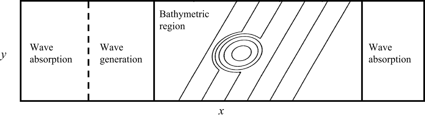
Figure 1. Schematic of lateral boundary condition treatment for the case of a shoal on a sloping beach.
In the adjoint model, we apply the adjoint lateral boundary conditions as
 \begin{equation} \begin{pmatrix} \lambda_1 \\ \lambda_2 \end{pmatrix}= c_r(x_r) \begin{pmatrix} \lambda_1 \\ \lambda_2 \end{pmatrix}. \end{equation}
Therefore,  $(\lambda _1,\lambda _2)$ is zero at the two ends of the computational domain to satisfy the periodic boundary conditions in the $x$ direction. In the $y$ direction, owing to the mirrored region, the adjoint boundary conditions are also periodic.
2.4. Sufficient measured information
Sections 2.2 and 2.3 introduce the adjoint system developed in this study for finding the optimal bathymetry  $\beta (x,y)$ to minimise the cost function $J$. However, a remaining important question is what measured information should be used to detect $\beta$. Fontelos et al. (Reference Fontelos, Lecaros, López and Ortega2017) theoretically proved the sufficiency of the free-surface elevation $\eta$, its first time derivative $\eta _t$, and the surface velocity potential $\varPhi ^s$ at a single time to uniquely determine the underlying bathymetry based on the potential flow theory. Vasan & Deconinck (Reference Vasan and Deconinck2013) showed high reconstruction accuracy for one-dimensional bathymetry by using the information of surface elevation $\eta$ and its two time derivatives, i.e. $\eta _t$ and $\eta _{tt}$, at a single time instant. However, the time derivatives are challenging to measure and can be easily contaminated by measurement noise in applications. Therefore, in our tests below, for the test cases that assume measurement without noise, we utilise the surface elevation and velocity potential at a single time instant and the surface elevation at the next available measured time instant as the measured information; for test cases of measurement with noise, we utilise more time instants of observed surface elevation. Our setting differs from the one-dimensional setting by Vasan & Deconinck (Reference Vasan and Deconinck2013) in that we consider measurements that may be contaminated by noise and use surface elevation information from only two consecutive time instants for perfect measurements. In contrast to the five-point finite-difference stencil used by Vasan & Deconinck (Reference Vasan and Deconinck2013), our time derivative calculation relies on less available information, a larger time interval, and potential measurement inaccuracies, leading to larger numerical errors. As a result, the error introduced by the time derivative calculation cannot be neglected in our case. In applications, the surface elevation and velocity potential can be obtained from the measured radial velocities using marine radar (Nwogu & Lyzenga Reference Nwogu and Lyzenga2010; Lyzenga et al. Reference Lyzenga, Nwogu, Beck, O'Brien, Johnson, de Paolo and Terrill2015).
2.5. Multiscale optimisation
With the gradient information calculated from the adjoint model in (2.28), the L-BFGS method (Byrd et al. Reference Byrd, Lu, Nocedal and Zhu1995; Zhu et al. Reference Zhu, Byrd, Lu and Nocedal1997) is then used to optimise the control parameters  $\beta (x,y)$ to reduce the cost function $J$ in (2.27). However, we find that the algorithm tends to overestimate the reconstructed bathymetry in the high-wavenumber region, as shown in the supplementary material. To solve this problem, we propose a treatment called multiscale optimisation. The main point of multiscale optimisation is to imitate the human sketching strategy to capture the large-scale structure of bathymetry first and then gradually refine the details. The following results show that our proposed multiscale treatment significantly improves the bathymetry reconstruction performance. The key step of the multiscale optimisation is an adaptive low-pass filter
 $$\begin{gather} \beta_{LP} = \mathcal{F}^{{-}1} [ \gamma_k(\theta_f) \mathcal{F} [\beta] ], \end{gather}$$
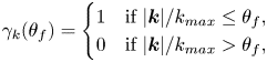 $$\begin{gather}\gamma_k(\theta_f) =\begin{cases} 1 & \text{if} \ |\boldsymbol k|/k_{max} \leq \theta_f,\\ 0 & \text{if} \ |\boldsymbol k|/k_{max}>\theta_f, \end{cases} \end{gather}$$
where  $k_{max}$ is the largest wavenumber available for the computational set-up, $\theta _f$ is the adjustable cutoff threshold ranging from 0 to 1, and $\beta _{LP}$ is the low-pass-filtered bathymetry. As shown in figure 2, the corresponding gradient for this treatment is
 \begin{equation} \frac{\partial J}{\partial \beta} = \mathcal{F}^{{-}1} \left[ \gamma_k(\theta_f) \mathcal{F} \left[\frac{\partial J}{\partial \beta_{LP}}\right] \right], \end{equation}
where the intermediate gradient  $\partial J / \partial \beta _{LP}$ is calculated using (2.28) and the final gradient $\partial J / \partial \beta$ is updated based on (2.34). In the first several optimisation iterations, $\theta _f$ is set to small values to capture the large-scale structures of $\beta$. In later iterations, we gradually increase $\theta _f$ to 1 to capture the fine details of $\beta$. We define $\theta _f$ at the $n$th iteration as
 \begin{equation} \theta_f = \min \{ n/1000+0.02,1 \}, \quad n=1,2,3\ldots. \end{equation}
We remark that the adjustable threshold  $\theta _f$ is not necessarily 1 when the optimisation process completes if the change in the cost function in two consecutive iterations is less than a threshold or the number of optimisation iterations reaches a predefined large value. The other potential alternative method to improve the performance of the reconstructed bathymetry is to add the regularisation term to penalise high wavenumber components in the cost function (e.g. Bewley, Moin & Temam Reference Bewley, Moin and Temam2001). However, the hyperparameters in the method are not trivial to tune to obtain the optimal results.
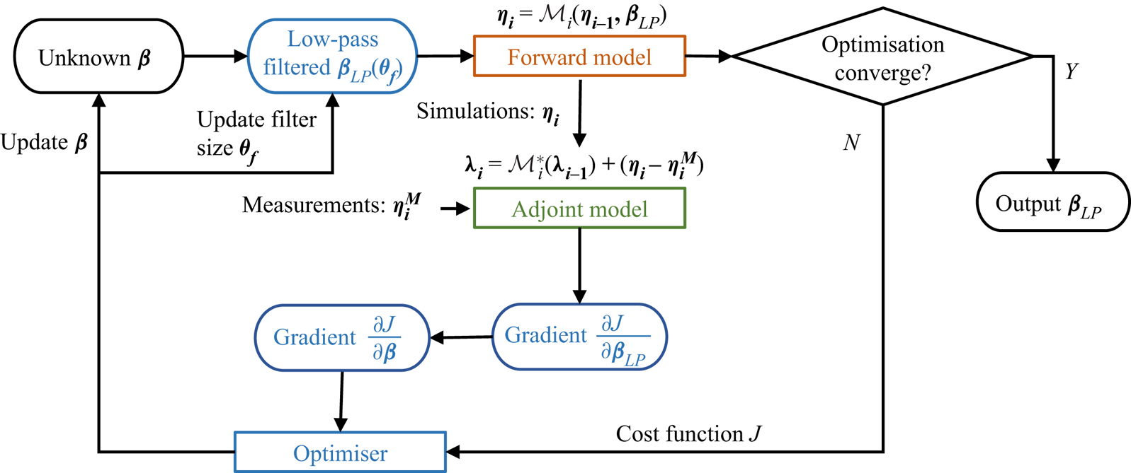
Figure 2. Bathymetry reconstruction algorithm based on the HOS method (brown), its adjoint model (green) and the multiscale optimisation (blue).
2.6. Bathymetry inversion algorithm
The bathymetry reconstruction problem is widely recognised to be ill-posed, primarily due to the presence of non-unique bottom solutions. In this context, we have endeavoured to alleviate these challenges through the careful design of surface observations in § 2.4, which aims at providing sufficient information to invert the bottom profile. Moreover, in § 2.5, we propose a multiscale optimisation scheme that is capable of effectively removing non-physical high-wavenumber bottom components, further improving the quality of the bottom reconstruction. The key steps to reconstruct and predict the wave field from the measurement are sketched in figure 2 and summarised below.
(i) Step 1. An initial guess for $\beta$ is given, and the low-pass-filtered $\beta _{LP}$ is calculated using (2.32) for starting the wave simulation.
(ii) Step 2. The HOS method is used for the forward simulation of the wave field from the initial time
$t_0$ to the final time $t_f$.(iii) Step 3. If the change in the cost function in two consecutive iterations is smaller than a threshold or the number of optimisation iterations reaches a predefined large value, the process ends, and
$\beta _{LP}$ is considered the optimal solution. Otherwise, we continue with Step 4.(iv) Step 4. The adjoint model is integrated from the final time
$t_f$ to the initial time $t_0$ to calculate the intermediate gradient $\partial {J}/\partial \beta _{LP}$ using (2.28).(v) Step 5. The final gradient
$\partial {J}/\partial \beta$ is calculated based on the intermediate gradient $\partial {J}/\partial \beta _{LP}$ using (2.34).(vi) Step 6. The cost function
${J}$ is calculated using (2.27). The gradient information and the cost function are fed into the multiscale optimisation method to optimise the bathymetry $\beta$ to reduce the cost function ${J}$.(vii) Step 7. We return to Step 2. A new optimisation iteration starts with the new bathymetry
$\beta _{LP}$ calculated from the modified bathymetry $\beta$ and the updated filter size $\theta _f$.


3. Performance of bathymetry inversion
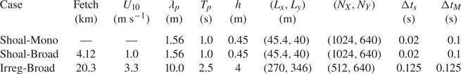
In this section, we evaluate the performance of our algorithm for two bathymetry feature types, shoal and irregular bathymetry, using monochromatic waves or broadband waves as the incident waves, as shown in table 1.
Table 1. Parameters of case set-up. Here, ‘Shoal’ and ‘Irreg’ represent shoal and irregular bathymetry, respectively; ‘Mono’ and ‘Broad’ represent monochromatic wave and broadband waves, respectively. The following variables are defined: surface wavelength,  $\lambda _p$; wave period, $T_p$; simulation domain length, $L_x$ and $L_y$; number of simulation grid points, $N_X$ and $N_Y$; simulation time interval, $\Delta t_s$; measurement time interval, $\Delta t_M$.
3.1. Reconstruction with monochromatic waves
We first apply our bathymetry inversion algorithm to a canonical case of the diffraction of a monochromatic wave over an elliptic shoal. We follow the design in a laboratory experiment by Berkhoff, Booy & Radder (Reference Berkhoff, Booy and Radder1982), which has been a benchmark test case widely used for validating numerical models for nonlinear wave and bottom interactions (e.g. Smith Reference Smith1998; Ricchiuto & Filippini Reference Ricchiuto and Filippini2014; Marche Reference Marche2020). The bathymetry features are characterised by a sloping plane, which has an oblique angle of 20 $^{\circ }$ with respect to the $y$-axis, surrounded by an ellipsoidal shoal (figure 3a). We introduce a coordinate system $(x',y')$ that is rotated by 20 $^{\circ }$ from the $(x,y)$ coordinate of the simulation
 \begin{equation} x' = x\cos{20^{{\circ}}}-y\sin{20^{{\circ}}},\quad y'=x\sin{20^{{\circ}}}+y\cos{20^{{\circ}}}. \end{equation}
With the reference water depth  $h=0.45$ m, the bathymetry spatial variation is defined by $\beta = z_b + z_s$, where
 $$\begin{gather} z_b(x',y') =\begin{cases} 0.02(x'+5.84) & \text{if } x'>{-}5.84, \\ 0 & \text{otherwise}, \end{cases} \end{gather}$$
 $$\begin{gather}z_s(x',y') =\begin{cases} -0.3+0.5\sqrt{1-\left(\dfrac{x'}{3.75}\right)^2-\left(\dfrac{y'}{5}\right)^2} & \text{if}\ \left(\dfrac{x'}{4}\right)^2+\left(\dfrac{y'}{3}\right)^2<1,\\ 0 & \text{otherwise}. \end{cases} \end{gather}$$
All lengths here are in metres. The incident waves have a period of 1 s and a wave height of 0.0464 m in the deep-water region. Figure 3(b) shows the surface elevation manifestation induced by the bottom.
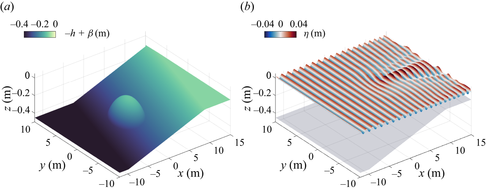
Figure 3. Monochromatic wave propagation over a shoal. (a) Shoal bathymetry  $-h+\beta (x,y)$; (b) surface elevation $\eta (x,y)$ at $t=36$ s.
For the simulation, the bathymetry geometry  $\beta$ described in (3.1)–(3.3) is embedded for $x\in [-12.4,15]$ m and $y\in [-10,10]$ m in the computational domain of $45.4~{\rm m}\times 40~{\rm m}$, as shown in table 1. A mirrored bathymetry with respect to $y=10$ m is given for $y\in [10,30]$ m. The bathymetry is extended to a flat region for $x\in [-24.4,-12.4]$ m and a sloping beach with a depth from 0.35 to 0 m for $x\in [15,21]$ m, similar to what was used in Smith (Reference Smith1998). As described in § 2.3, two wave absorption zones at $x\in [-24.4,-18.4]$ m and $x\in [15,21]$ m are placed near the inlet and outlet boundaries of the computational domain, respectively, and a wave generation zone at $x\in [-18.4,-12.4]$ m is included near the left-hand inlet boundary.
We first examine the performance of the HOS method for the forward wave simulation. As shown in figure 4, we compare the HOS simulation using nonlinear perturbation orders  $M=3$ and $M=5$ with the measured wave height at eight transects in Berkhoff et al. (Reference Berkhoff, Booy and Radder1982). The wave height is defined as the difference between the maximum and minimum surface elevations. Figure 4 shows that the simulation using the high nonlinear perturbation order ( $M=5$) agrees well with the measurement by Berkhoff et al. (Reference Berkhoff, Booy and Radder1982), while the results from the low nonlinear perturbation order ( $M=3$) exhibit deviations from the measurement. This result is consistent with the previous observation that it is necessary to have a high nonlinear perturbation order ( $M>3$) to accurately simulate wave evolution over complex bathymetry features for nonlinear perturbation-based methods (Guyenne & Nicholls Reference Guyenne and Nicholls2008; Gouin et al. Reference Gouin, Ducrozet and Ferrant2016), which indicates the importance of the high-order terms in the wave–bottom interaction simulations and thus the necessity to incorporate these terms into the inversion algorithms. Our proposed reconstruction method has the capability of accommodating a high nonlinear perturbation order. Our tests with other nonlinear perturbation orders $M=4,5,6$ show that $M=5$ is adequate (results not shown here for space consideration). In the following sections, we use $M=5$ for both the HOS method and the adjoint equations.
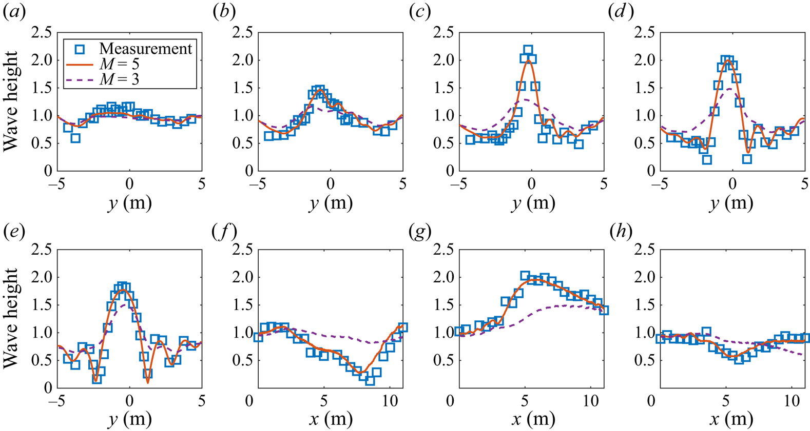
Figure 4. Comparison of our HOS simulations using  $M=5$ or $M=3$ with the measurement in Berkhoff et al. (Reference Berkhoff, Booy and Radder1982). The wave height is normalised by that of the incident wave, 0.0464 m. The locations of the transects are (a) $x=1$ m; (b) $x=3$ m; (c) $x=5$ m; (d) $x=7$ m; (e) $x=9$ m; ( f) $y=-2$ m; (g) $y=0$ m; (h) $y=-2$ m.
For the bathymetry reconstruction, we choose the measurement sampling frequency as 10 Hz with  $\Delta t_M=0.1$ s in table 1, which is in the range of the ocean wave radar measurement sampling frequency (Ewans, Feld & Jonathan Reference Ewans, Feld and Jonathan2014). As discussed in § 2.4, we use wave states $\eta |_{t_0}$, $\varPhi |_{t_0}$ and $\eta |_{t_0+\Delta t_M}$ to detect the bathymetry, where $t_0$ can be an arbitrary time instant. For the presentation of the results, we set $t_0=36$ s, where $t=0$ corresponds to the time instant at which our simulation begins. We have tested the algorithm performance using different choices of $t_0$, and the results obtained are similar. To provide an overview of the gradient of the cost function with respect to the bathymetry, figure 5(a) presents $\partial J/\partial \beta$ at the initial guess $\beta =0$ calculated by (2.28). In addition to the bathymetric characteristics, such as the elliptical shape near $(0,0)$ and the tilted sloping plane, the gradients also share similar surface wave characteristics, such as the sinusoidal shape and the surface distortion pattern. The surface wave-induced sensitivity introduces high-wavenumber components at the surface wavelength scales, which do not exist in the true bathymetry. Similar observations of the high-wavenumber oscillation are also obtained in the reconstructed bathymetry as shown in the supplementary material, unless our proposed multiscale optimisation treatment is employed (§ 2.5).
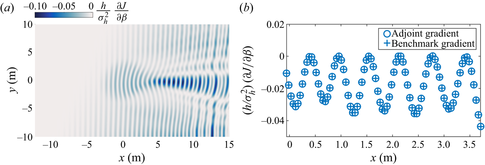
Figure 5. (a) Gradient of the cost function with respect to the bathymetry at the initial guess  $\beta =0$; (b) comparison between the adjoint gradient by the adjoint model in (2.28) and the benchmark gradient calculated using the finite difference method in (3.4) on 86 grid points along the horizontal line $y=0$ m. The gradient is normalised by the standard deviation of the surface elevation at the initial time instant $\sigma _\eta =0.014$ m and $h =0.45$ m.
To verify the calculation of adjoint gradients, we compare them with the gradients calculated directly using the finite difference method. The latter is treated as the benchmark solution of the gradients and is obtained using a finite difference scheme, in which the gradient of the cost function with respect to  $\beta$ at any point $(i,j)$ is calculated as
 \begin{equation} \left.\frac{\partial {J}}{\partial \beta (i,j)} \right|_{Benchmark} = \frac {{J}_{\beta+\delta}-{J}_{\beta}}{\delta}, \end{equation}
where  ${J}_{\beta }$ is calculated by (2.27) with $\beta$ and where ${J}_{\beta +\delta }$ is calculated by adding a small perturbation $\delta$ to $\beta (i,j)$. We set the magnitude of $\delta$ to be $1.0\times 10^{-4}$ m, which is sufficiently small to reduce the error caused by the finite difference approximation. Figure 5(b) shows a comparison of the gradients at 86 grid points along the line $y=0$ m near the bump at the initial guess of $\beta =0$. There is good agreement between the adjoint gradients calculated using (2.28) and the gradients calculated by the finite difference method using (3.4). We have also compared the gradients at other locations and have found good agreement.
To illustrate the bathymetry reconstruction performance, we present in figure 6 the result after the cost function has converged after 400 optimisation iterations. A reference depth  $h$ is required by the HOS method for water wave time evolution, and, as a result, our algorithm requires an estimate of $h$ beforehand. Similarly, Nicholls & Taber (Reference Nicholls and Taber2009) also required an estimate of $h$ in the Dirichlet–Neumann operator for their reconstruction algorithm, while Vasan & Deconinck (Reference Vasan and Deconinck2013) only needed a reference depth above the bathymetry and solved the initial value problem for Laplace's equation in the vertical direction to find the bottom location. Our bottom reconstruction algorithm does not necessarily require an accurate a priori estimate of $h$ and the discrepancy in $h$ can be rectified by adjusting the bottom profile $\beta$ as long as the HOS method converges. In future work with the increase in computer power, more simulations with varying initial estimates of $h$ can be conducted to quantitatively and systematically evaluate the validity range and impact of this parameter on bottom reconstruction performance. Figure 6(a) shows the reconstructed bathymetry, which agrees with the ground truth well as shown in figure 3(a). For quantitative comparison, figure 6(b,c) shows good agreement between the reconstructed bathymetry elevation and ground truth along lines $x=0$ m and $y=0$ m, respectively.

Figure 6. (a) Reconstructed bathymetry after 400 optimisation iterations; (b) comparison of reconstructed bathymetry and ground truth along the line  $x=0$ m; (c) same as (b) but for the line along $y=0$ m.
To quantitatively assess the reconstruction performance, we define a relative error based on the  $L^2$ norm as
 \begin{equation} \epsilon_\beta = \frac{\|\beta_d-\beta \|_{2}}{\|\beta\|_{2}}, \end{equation}
where  $\beta _d$ denotes the reconstructed bathymetry and $\beta$ is the ground truth. Because we use an initial guess of $\beta _d=0$ at the beginning of the optimisation, the initial value of the relative reconstruction error $\epsilon _\beta$ is one. Figure 7 shows the decrease in the cost function and detection error with iterations, resulting in less than 1 % of their original values at the end of optimisation. The results confirm the effectiveness of the proposed multiscale optimisation method, which leads to a 99.6 % reduction in detection error and a 99.75 % reduction in the cost function compared with the results without using the multiscale method as shown in the supplementary material.
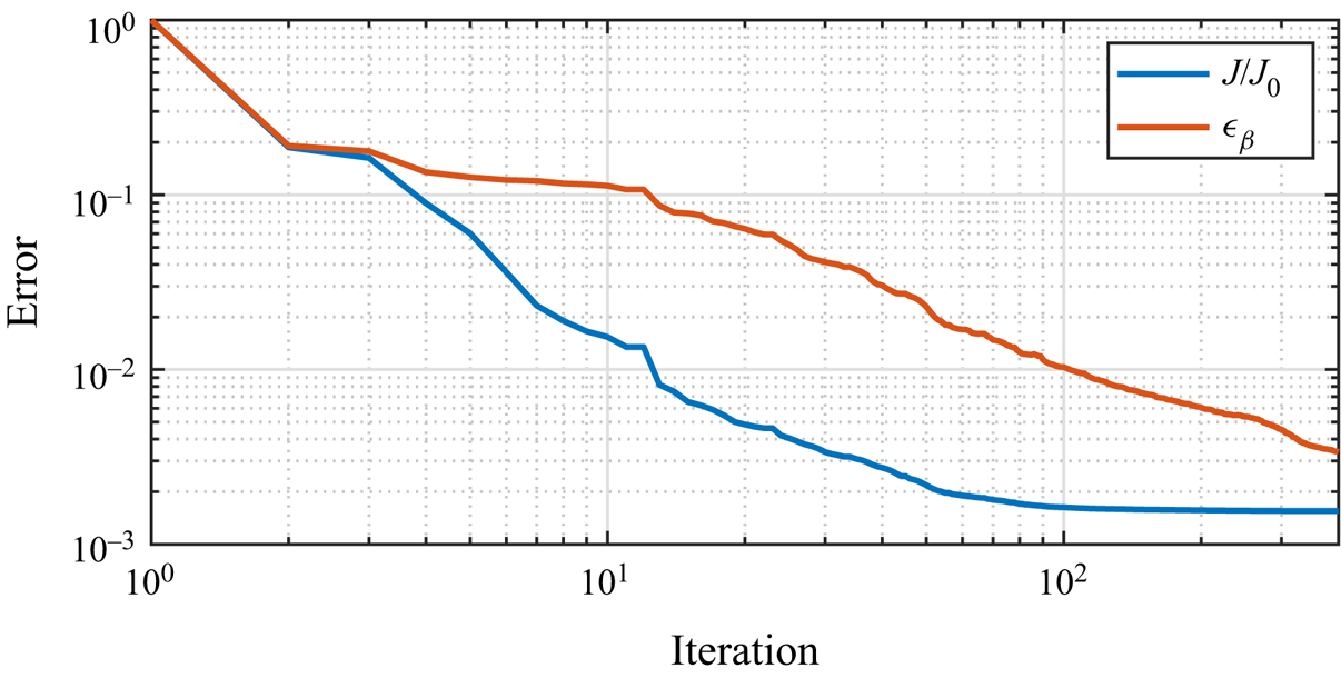
Figure 7. Variations of cost function and detection error with the number of optimisation iterations with multiscale optimisation method for case Shoal-Mono.
3.2. Reconstruction with broadband waves
In this section, we consider a more general problem in the coastal environment for the reconstruction of bathymetry with multidirectional broadband waves. The incident wave field is constructed from the directional Joint North Sea Wave Project (JONSWAP) spectrum (Hasselmann et al. Reference Hasselmann1973)
 \begin{equation} S(\omega,\theta)=\frac{\alpha g^2}{\omega^5}\exp\left[-\frac{5}{4}\left(\frac{\omega} {\omega_p}\right)^ {{-}4}\right]\gamma^{\exp[-{(\omega-\omega_p)^2}/{(2\sigma^2\omega_p^2)}]}D(\theta) , \end{equation}
where  $\alpha$ is the Phillips parameter, $\omega$ is the wave frequency, $\omega _p$ is the peak wave frequency, $\lambda _p$ is the peak wavelength, $T_p$ is the peak wave period, $\gamma =3.3$ is the peak-enhancement parameter, $\sigma =0.07$ for $\omega \leq \omega _p$, $\sigma =0.09$ for $\omega >\omega _p$, and $D(\theta )=2\cos ^2(\theta )/{\rm \pi}$ with $\theta \in [-{\rm \pi} /2,{\rm \pi} /2]$ is the angular spreading function. The parameter $\alpha$ and wave frequency $\omega _p$ are calculated as
 \begin{equation} \alpha = 0.076\left(\frac{U^2_{10}}{Fg}\right)^{0.22}, \quad \omega_p = 22\left(\frac{g^2}{U_{10}F}\right)^{1/3}, \end{equation}
where  $g$ corresponds to gravity acceleration with a value of 9.8 m s $^{-2}$, $U_{10}$ is the wind speed 10 m above the mean water surface, and $F$ is the fetch. As shown in table 1, we choose $U_{10}$ of 1 m s $^{-1}$ and $F$ of $4.12$ km such that the peak wavelength and the peak wave period are the same for those in the monochromatic wave case with $\lambda _p=1.56$ m and $T_p=1$ s. We first perform an auxiliary simulation where the initial wave field evolves for a sufficiently long time over a constant water depth $h=0.45$ m ( $k_p h = 1.81$) and then input the simulated broadband waves as the incident waves in the wave generation zone of
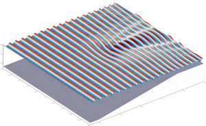
  $x\in [-18.4,-12.4]~\mathrm {m}$. Compared with the long waves, the short waves barely interact with the bathymetry and can be seen as a type of noise in bathymetry reconstruction. In this study, the short waves are present because of the high resolution used in our forward simulations. The bathymetry reconstruction does not rely on these short waves, and thus we expect our algorithm to perform well for data with a coarser resolution. However, the existence of these short waves is still meaningful because they demonstrate the robustness of our algorithm against noise.
Figure 8(a) shows an instantaneous surface elevation field for broadband wave propagation over the shoal. Contrary to the strong surface manifestation induced by bathymetry variations on the monochromatic wave shown in figure 3(b), the bathymetry does not introduce a prominent surface pattern for broadband waves. Figure 8(b) shows the gradient  $\partial J/\partial \beta$ at the initial guess $\beta =0$. We can observe that the gradient contains both the characteristics of the bathymetry variation and the surface waves; for example, the almost-zero values for $x<0$ m are consistent with the flat regions of $\beta$ and the surface pattern of broadband waves for $x>5$ m. However, these characteristics are less distinct compared with those of the monochromatic wave shown in figure 5(a).

Figure 8. Broadband waves propagating over the shoal. (a) Surface elevation at  $t=50$ s; (b) gradient of cost function with respect to the bathymetry at the initial guess $\beta =0$. In (b), the results are normalised by ${\sigma _\eta =0.0095}$ m and $h=0.45$ m.
We utilise the surface elevation and velocity potential at  $t=50$ s and another snapshot of surface elevation at $t=50.1$ s to test the bathymetry inversion algorithm performance. Figure 9(a) plots the reconstructed bathymetry for broadband waves after 400 iterations. We also show a comparison between the reconstruction results and the ground truth along the two lines $x=0$ m and $y=0$ m in figure 9(b,c), respectively. The reconstructed bathymetry recovers the ground truth well for most of the locations except for some oscillations near the left-hand inlet, $x=-12.4$ m. This is because of the numerical treatment of the inlet boundary conditions described in § 2.3. We nudge the simulated waves to the prescribed incident wave conditions in the wave generation zone $x\in [-18.4,-12.4]$ m, and thus the bathymetry variation in the wave generation zone has less impact on the surface waves, which results in a higher reconstruction error. Figure 10 plots the variations of the normalised cost function and detection error with optimisation iterations. The normalised cost function decreases continuously with iterations, reaching a value close to 0.1 %. In contrast, the detection error first decreases to less than 1 % with iterations and then exhibits a slight increase, which may indicate an overfitting phenomenon.

Figure 9. The legend is the same as in figure 6. The results for the Shoal-Broad case are plotted.

Figure 10. Variations of cost function and detection error with the number of optimisation iterations with multiscale optimisation method for case Shoal-Broad.
3.3. Detection of field-scale irregular bathymetry
In this section, we apply our method to the reconstruction of irregular bathymetry in a field case. We use the bathymetry data extracted from a field experiment in Duck, North Carolina, USA reported by Moulton et al. (Reference Moulton, Elgar, Raubenheimer, Warner and Kumar2017). As shown in figure 11(a), the bathymetry variation is characterised by an irregular slope and a concave channel. The field conditions in Moulton et al. (Reference Moulton, Elgar, Raubenheimer, Warner and Kumar2017) are incorporated into our computational domain of size  $150~ {\rm m} \times 346~{\rm m}$, as shown in table 1. The bathymetry features extend to a flat region for $x<0$ m and a sloping plane for $150~{\rm m} < x<190~{\rm m}$. Two wave absorption zones of width $L=40$ m are placed near the inlet and outlet boundaries of the computational domain, and a wave generation zone of width $L=40$ m is added near $x=0$ m. Owing to the requirement for wave simulations of $-h+\beta <\eta$ from (2.1), we set the water depth $h=4$ m to ensure that the bathymetry is always underwater (because the run-up of waves on beaches is beyond the scope of this study), but the spatial variation $\beta$ is kept the same. The domain is mirrored with respect to $y=173$ m to satisfy the periodic boundary conditions in the $y$ direction.
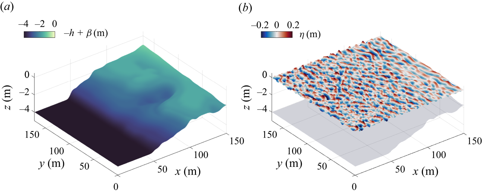
Figure 11. Broadband waves propagating over field-scale irregular bathymetry. Plotted are contours of the (a) bathymetry  $-h+\beta (x,y)$ and (b) surface elevation $\eta (x,y)$ at $t=100$ s.
As shown in table 1, the broadband waves are constructed from the JONSWAP spectrum with  $U_{10}=3.3$ m s $^{-1}$ and $F=20.3$ km, which results in a wave field with a peak wavelength $\lambda _p$ of 10 m and a peak wave period $T_p$ of 2.5 s. The wave field in the generation zone is produced from an auxiliary simulation, similar to § 3.2. The wave evolution is simulated using the HOS method with $M=5$. Figure 11(b) plots a snapshot of the broadband waves over the irregular bathymetry. Similarly, as shown in figure 8(a), it is not easy for the naked eye to see how the spatial variations in the bathymetry induce manifestations in the surface waves. Figure 12(a) plots the reconstructed irregular bathymetry using our inversion algorithm after 400 iterations, and figure 12(b,c) shows a comparison between the reconstructed bathymetry data and the ground truth for two cross-sections at the concave channel. Figure 12 shows that the reconstructed bathymetry agrees well with the ground truth. Owing to the page limit, the evolution of the reconstructed bathymetry with optimisation iterations is depicted in the supplementary movie. Figure 13 depicts the variations of the normalised cost function and detection error with optimisation iterations. Both the normalised cost function and detection error decrease continuously with iterations, achieving values less than 10 % and 1 %, respectively.

Figure 12. (a) Reconstructed bathymetry after 400 optimisation iterations for case Irreg-Broad; (b) comparison of reconstructed bathymetry and the ground truth along the line  $x=100$ m; (c) same as (b) but for the line along $y=70$ m.
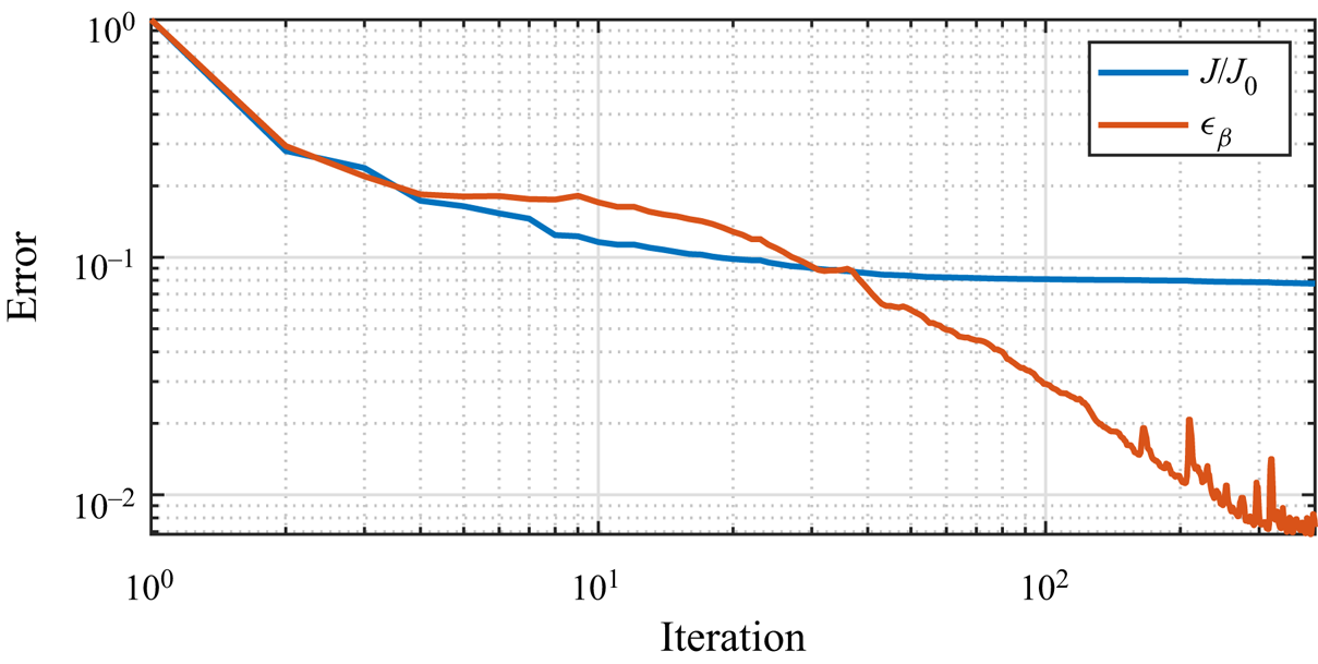
Figure 13. Variations of cost function and detection error with the number of optimisation iterations with multiscale optimisation method for case Irreg-Broad.
4. Effects of the sampling frequency and measurement noise
In § 3, we show that noise-free surface wave measurements at a sampling frequency of  $\sim$10 Hz are sufficient for our inversion algorithm to obtain satisfactory bathymetry reconstruction results for both monochromatic and broadband incident waves with peak wave frequencies of $\sim$1 Hz. In this section, we further examine the algorithm performance in a more realistic situation involving the effects of limited sampling frequency and measurement noise.
4.1. Effect of the sampling frequency
To investigate the effect of the sampling frequency, we choose the measurement  $\eta |_{t_0+\Delta t_M}$ at different measurement time intervals $\Delta t_M={0.02,0.1,0.2,0.4,0.6,0.8}$ s for the Shoal-Mono and Shoal-Broad cases for bathymetry reconstruction while keeping the other parameters the same as those in table 1. Figure 14 presents the reconstruction errors with different sampling frequencies for the Shoal-Mono and Shoal-Broad cases. The algorithm performance is robust, with reconstruction errors less than 1.5 % for all different choices of measurement time intervals in the range of $\Delta t_M/T_p\le 0.8$, where $T_p=1$ s for both monochromatic and broadband waves. We remark that the seemingly counter-intuitive good bathymetry detection performance under large measurement time intervals is related to the usage of the entire wave state at the first time instant. Given the wave state (including the surface elevation and surface velocity potential) at the earliest time instant, the observed wave state at the later time instants can be a good indicator of the bathymetry even though the time interval is large. Moreover, we focus on the effect of the sampling frequency by neglecting the measurement noise effect in this section, and we anticipate that the reconstruction error increases as the measurement time interval increases if the measurement noise is taken into account. The reconstruction errors in the broadband wave cases are slightly larger than those in the monochromatic wave cases, which is consistent with the less prominent surface manifestation and more irregular gradient $\partial J/\partial \beta$ present in broadband waves, as shown in figure 8. Nevertheless, the bathymetry can still be reconstructed with satisfactory accuracy ( $\sim$1.4 % error) with multidirectional broadband waves.

Figure 14. Relative reconstruction error  $\epsilon _\beta$ for different sampling frequencies for the Shoal-Mono and Shoal-Broad cases.
4.2. Effect of measurement noise
In this section, we consider the effect of measurement noise on the bathymetry reconstruction performance. We generate synthetic surface wave data with random noise added to the true surface elevation as
 \begin{equation} \eta_{M}(x,y,t) = \eta(x,y,t) + \mu(x,y,t), \end{equation}
where the noise  $\mu (x,y,t)$ satisfies the Gaussian distribution with standard deviation $\sigma _{noise}$. To exclude the effect of inaccurate initial conditions on the inverse problem, we prescribe the wave state at $t=t_0$ using the accurate solution and perturb the surface elevation at later time instants with random noise. In this case, the perturbed surface elevation at a single time instant is insufficient to accurately recover the bathymetry. To reduce the effect caused by the noise, we choose snapshots of the perturbed surface elevation at five time instants to recover the bathymetry in the following discussion.
Figure 15 illustrates how the cost function and relative reconstruction error vary with the optimisation iteration for broadband waves over the shoal described in § 3.2. We set up three more cases with different levels of noise, of which the standard deviations are  $\sigma _{noise}/\sigma _\eta = 10\,\%, 20\,\%$ and $30\,\%$. We choose the cutoff iteration at 400, at which the cost function $J$ has converged. The normalised cost function (figure 15a) decreases with additional optimisation iteration, and the converged normalised cost function increases from 0.15 % to 20 % with an increasing noise level $\sigma _{\text {noise}}/\sigma _\eta$ from 0 to 30 %. In contrast, the reconstruction error (figure 15b) first decreases with additional optimisation iteration and then increases, which suggests an overfitting phenomenon in all cases. With the increase in noise levels, the smallest reconstruction errors increase, and the critical iteration number, at which the smallest error occurs, decreases. This qualitative feature is related to the surface wave-induced high-wavenumber components in the gradient $\partial J/\partial \beta$. For large numbers of iterations, the obtained optimal $\beta$ overfits the noisy wave observations by containing spurious high-wavenumber components that do not exist in the ground truth bathymetry data. Consequently, the error increases with an increasing noise level because there is more energy in the high-wavenumber modes induced by the measurement noise; therefore, the overfitting becomes more severe.
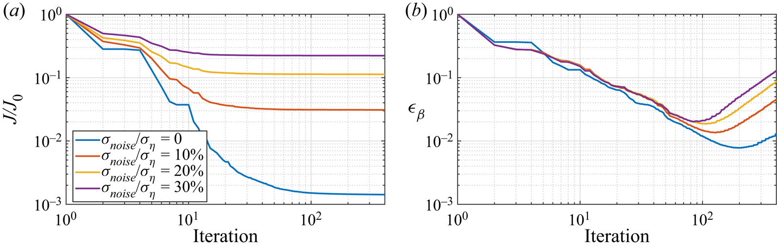
Figure 15. (a) Cost function  $J$ and (b) relative reconstruction error $\epsilon _\beta$ as functions of the optimisation iteration numbers for measurement with noise. In (a), the cost function $J$ is normalised by $J_0$, its initial value before the optimisation process.
In figure 16, we plot representative  $\beta$ obtained during early iterations, near the critical iteration, and at the final iteration for the case with the highest noise level at $\sigma _{noise}/\sigma _\eta = 30\,\%$. We find that the reconstructed bathymetry can capture the main characteristics, such as the slope and bump, after 20 iterations, which addresses approximately $4\,\%$ of the degrees of freedom in the physical space of the original bathymetry data. Next, after 90 iterations, the bathymetry can be refined with a reconstruction error of approximately 2 %. When the number of iterations further increases to 400, the reconstructed bathymetry geometrically fits the ground truth. However, abundant oscillations exist on the bathymetry obtained. Note that the surface wave dynamics are not affected by these bottom variations of short length scales. The cost function remains nearly the same between 90 iterations and 400 iterations, as shown in figure 15(a). To mitigate the overfitting with noisy data, some empirical knowledge or an approximate estimate of the length scales of the bathymetry data $\beta$ would be beneficial to determine the cutoff $\theta _f$ in (2.33), such that the high-wavenumber components in figure 16(c) can be avoided.

Figure 16. Reconstructed bathymetry for the Shoal-Broad case with  $\sigma _{noise}/\sigma _\eta =30\,\%$ after (a) 20 iterations; (b) 90 iterations; (c) 400 iterations.
5. Effects of small bottom variations and limited measurements
In this section, we evaluate the performance of our algorithm in the scenario of small bottom variations and a limited number of measurements.
5.1. Algorithm performance with small bottom variations
To evaluate the performance of our algorithm with small bottom variations, we apply it to a canonical case of a monochromatic wave propagating over a Gaussian bump. This scenario was investigated by Nicholls & Taber (Reference Nicholls and Taber2009) and Khan & Kevlahan (Reference Khan and Kevlahan2021) previously. The prescribed bottom profile is given by
 \begin{equation} \beta(x) = b \,{\rm sech}(2x), \end{equation}
where the bottom variation amplitude is  $b=0.02$ m and the water depth $h$ is set to 0.2 m, resulting in a small bottom variation ratio $b/h=0.1$. A monochromatic wave with a wave period 1 s and wave height 0.0464 m propagates from the $-x$ to $+x$ direction. To facilitate the simulation of the incident wave condition, as discussed in § 2.3, we introduce zones for wave generation and absorption, each has 6 m in length, extending the computational domain from 10 m to a total of 28 m. The other computational parameters can be found in table 2.
Table 2. Parameters of the case set-up for bathymetry inversion in the scenario of a monochromatic wave over a Gaussian bump. The following variables are defined: simulation grid length,  $\Delta x_s$; measurement grid length, $\Delta x_M$; measurement starting time instant, $T_s$; measurement ending time instant, $T_e$.
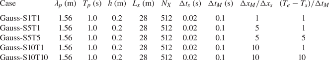
For the bathymetry reconstruction, we employ a measurement sampling interval of  $\Delta t_M=0.1$ s (table 2). To evaluate the performance of the bathymetry inversion algorithm, we utilise the surface elevation and velocity potential data at $t=30$ s, along with the subsequent observed snapshot of surface elevation at $t=30.1$ s. Figure 17(a) presents the results of the optimisation process, showcasing the decreases in the cost function and detection error with iterations. At the end of the optimisation, the cost function and detection error decrease to approximately $10^{-4}$ and $10^{-2}$ of their original values, respectively. The phenomenon that the cost function remains nearly constant and the bathymetry is not updated much before 100 iterations can be attributed to the small bottom variations in the problem configuration. As discussed in § 2.5, our multiscale optimisation method prioritises capturing the large-scale structures in the early stage of optimisation. For the local variations, the minimisation process takes effect primarily in the optimisation iterations later. In figure 17(b), we depict the comparison between the detected bathymetry and the ground truth, further confirming the algorithm's satisfactory performance in addressing the scenario of small bottom variations.
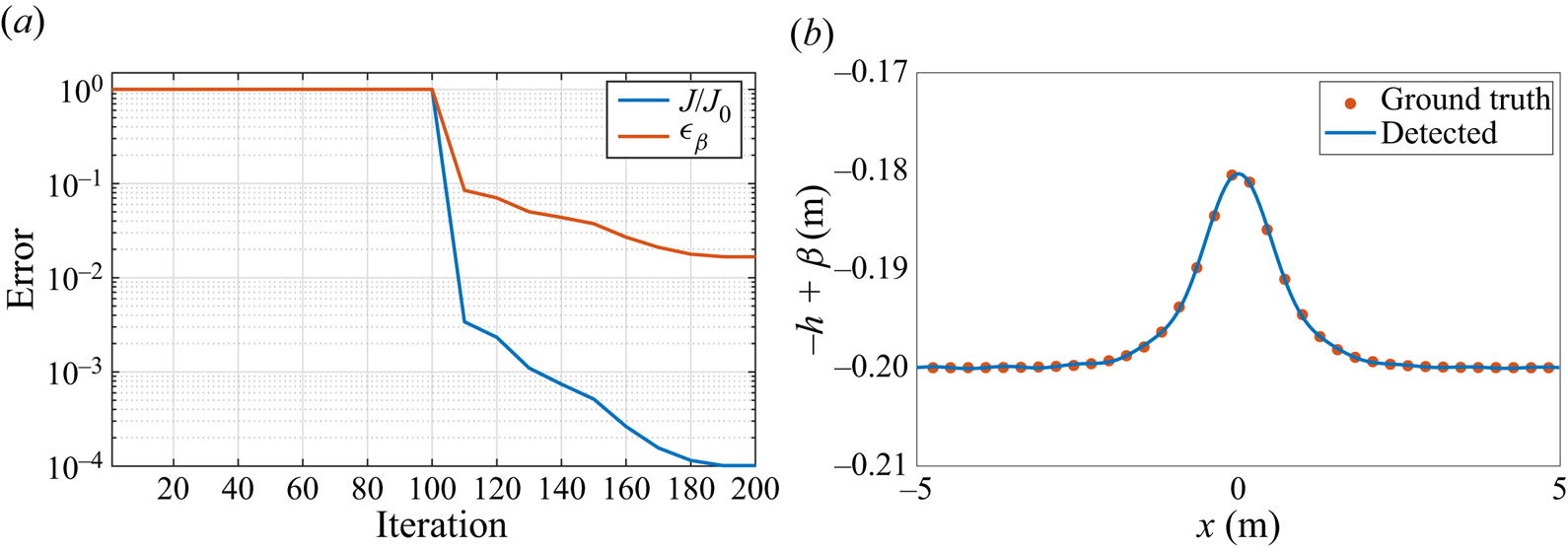
Figure 17. (a) Variations of the cost function and detection error with the number of optimisation iterations. (b) Comparison of the reconstructed bathymetry and ground truth. Results are plotted for case Gauss-S1T1.
5.2. Algorithm performance with limited measurements
In this section, we analyse the performance of the algorithm when there are only a limited number of measurements. We design three test cases with different degrees of sparsity in the observations, which is characterised by the parameter  $\Delta x_M/\Delta x_s$ ranging from 1 to 10, where $\Delta x_M$ represents the spatial distance between the observation points and $\Delta x_s$ refers to the grid length in the simulation (see cases Gauss-S1T1, Gauss-S5T1 and Gauss-S10T1 in table 2). It is important to note that, as discussed in § 2.4, sparse observations at a single time instant are insufficient to uniquely determine the bathymetry. To address the challenges arising from sparse observations, we investigate two additional cases with an increased number of observation time instances, calculated as $(T_e-T_s)/\Delta t_M$, based on different sparsity levels. These cases are denoted as Gauss-S5T5 and Gauss-S10T10 in table 2.
Figure 18(a) presents a comparison between two cases, Gauss-S5T1 and Gauss-S5T5, regarding their cost function and detection error. Gauss-S5T1 utilises observations from a single time instant, while Gauss-S5T5 benefits from observations spanning five time instants, both with a data sparsity level of  $\Delta x_M/\Delta x = 5$. Throughout the optimisation iterations, the two cases exhibit a similar trend of decreasing cost function and detection error. By the end of the optimisation process, the cost function and detection error saturate at similar values as case Gauss-S1T1 shown in figure 17. For further insight, in figure 18(b), we provide a comparison of the detected bottom with the ground truth for cases Gauss-S5T1 and Gauss-S5T5. Both cases demonstrate that the reconstructed bathymetry agrees well with the ground truth, indicating the robustness and effectiveness of our algorithm when handling data that are 80 % less.

Figure 18. Legends are the same as in figure 17. Results are plotted for cases Gauss-S5T1 and Gauss-S5T5.
In figure 19, we present the performance of our algorithm for cases Gauss-S10T1 and Gauss-S10T10. Figure 19(a) shows that, by the end of the optimisation iteration, the detection error for case Gauss-S10T1 becomes evident, saturating at 10 %, primarily due to the scarcity of observation data, which is reduced by 90 %. However, a noticeable improvement is observed with an increase in the number of observation snapshots, resulting in a reduced detection error of 2 % for Gauss-S10T10. Moreover, as shown in figure 19(b), there is a noticeable difference between the ground truth and the result obtained solely from a single time instant in case Gauss-S10T1. In contrast, the reconstructed bathymetry in case Gauss-S10T10 agrees well with the ground truth, demonstrating the effectiveness of incorporating more measurement snapshots and the robustness of our algorithm in the challenging scenario of increasing data sparsity.

Figure 19. Legends are the same as in figure 17. Results are plotted for cases Gauss-S10T1 and Gauss-S10T10.
6. Summary and discussion
In this study, we propose an adjoint-based variational data assimilation method for inferring coastal bathymetry from surface wave data. In our approach, we utilise the HOS method to simulate nonlinear wave propagation over variable bathymetry. We derive the recursion-formed adjoint HOS equations with the capability of accommodating any given nonlinear perturbation order, based on which we obtain the gradient expression of the cost function with respect to the bathymetry. We further propose a multiscale optimisation method that combines the L-BFGS optimiser with a size-adjustable low-pass filter to obtain satisfactory bathymetric reconstruction results.
To evaluate the algorithm performance, we conduct test cases considering different bathymetry feature types, surface waves, measurement sampling frequencies and measurement noise. We first consider a benchmark case of wave diffraction over a shoal on an oblique sloping beach. We find that it is necessary to utilise a high nonlinear perturbation order ( $M=5$) to accurately predict the nonlinear wave evolution over the bathymetry features. This result indicates the importance of nonlinear terms in wave–bottom interactions, for which our method has the advantage of accommodating an arbitrarily high nonlinear perturbation order. The gradients of the cost function with respect to the bathymetry calculated using the adjoint model are validated against the values obtained from a finite difference method. We find that the gradient distribution exhibits the characteristics of both the bathymetry and the surface waves, which are at different length scales. With the multiscale optimisation method, excellent reconstruction results are obtained for monochromatic incident waves, broadband waves, laboratory-scale shoals on an oblique sloping beach and field-scale irregular bathymetry data extracted from field measurements. We also tested the algorithm performance for different measurement sampling frequencies. We find that the algorithm can produce good reconstruction results with errors less than 1.5 % for a wide range of wave observation sampling time intervals. It is also found that the algorithm can still produce good results when the measurement is contaminated by noise. However, a priori knowledge or an empirical estimate of the length scales in the bathymetry data $\beta$ would be beneficial to mitigate the overfitting that arises with noisy data. Additionally, we demonstrate the robustness of our algorithm in the scenarios of small bottom variations and a limited number of measurements.
We note that the performance of the proposed algorithm is tested using the surface wave information  $\eta |_{t_0}$, $\varPhi ^s|_{t_0}$ and $\eta |_{t_0+\Delta t_M}$, which can be obtained from the measured radial velocities from marine radars (Nwogu & Lyzenga Reference Nwogu and Lyzenga2010; Lyzenga et al. Reference Lyzenga, Nwogu, Beck, O'Brien, Johnson, de Paolo and Terrill2015). Moreover, the algorithm can also accommodate other measurement types with straightforward modifications, although it remains an open question whether the exact bathymetry can be recovered owing to the unknown sufficiency of the measurement provided (Fontelos et al. Reference Fontelos, Lecaros, López and Ortega2017).
While our bottom reconstruction algorithm shows promising results for both laboratory and field-scale bathymetry under monochromatic and broadband wave scenarios, we emphasise that there is a need, with the increase in computer power to enable more extensive computations, for studies to further test the limits of its performance. Specifically, we plan to conduct simulations to assess the accuracy and robustness of our method under extreme cases where the reconstruction error is likely to be large, such as small relative amplitude of irregular bathymetry, limited number of measurements, and measurement location outside the support of bathymetry. We believe that such analyses will provide insight into the useful range of applications of our method and identify areas for potential improvement. Additionally, we will conduct simulations to evaluate the algorithm's accuracy and robustness for a range of sparse observation configurations, with different relative amplitudes of irregular bathymetry. With that, we can further directly compare with the results reported by Khan & Kevlahan (Reference Khan and Kevlahan2021, Reference Khan and Kevlahan2022) who considered similar scenarios and demonstrated the effectiveness of their method using the variational data assimilation technique. Finally, we emphasise that the present study focuses on the mathematical formulation, algorithm development and numerical tests with synthetic wave data. More studies in the future are needed to further test our model with real wave data, for which laboratory and field measurement studies are necessary.
Supplementary material and movie
Supplementary material and movies are available at https://doi.org/10.1017/jfm.2023.733.
Acknowledgements
The support of the Office of Naval Research to this research is gratefully acknowledged.
Funding
This work is supported by the Office of Naval Research.
Declaration of interests
The authors report no conflict of interest.
Appendix A. Derivation of the adjoint model and gradients
Let  $\boldsymbol {\mathcal {M}}(\boldsymbol {q})=\boldsymbol {0}$ denote the nonlinear wave model, where $\boldsymbol {q}=[\eta, \varPhi ^s, W]^{\text {T}}$ with the superscript $\text {T}$ denoting the transpose. Specifically, $\boldsymbol {\mathcal {M}}(\boldsymbol {q})=\boldsymbol {0}$ can be interpreted as reorganising (2.10)–(2.12) by moving all the terms to the left-hand side of the equations. A small perturbation $\delta \beta$ to the bathymetry $\beta$ result in a perturbation $\delta \boldsymbol {q} = [\delta \eta,\delta \varPhi ^s, \delta W]^{\text {T}}$. Let $\boldsymbol {\mathcal {M}}' (\boldsymbol {\delta q}) =\boldsymbol {0}$ denote the linearised wave model that governs the evolution of perturbation $\delta \boldsymbol {q}$ resulting from given perturbation $\delta \beta$. Specifically, $\boldsymbol {\mathcal {M}}' (\boldsymbol {\delta q}) =\boldsymbol {0}$ includes three parts, namely, $\delta \eta _t$, $\delta \varPhi ^s_t$ and $\delta W$, as
 $$\begin{gather} \delta \eta_t + \boldsymbol{\nabla} \delta \varPhi^s \boldsymbol{\cdot} \boldsymbol{\nabla} \eta + \boldsymbol{\nabla} \varPhi^s \boldsymbol{\cdot} \boldsymbol{\nabla} \delta \eta - (1+\boldsymbol{\nabla} \eta \boldsymbol{\cdot} \boldsymbol{\nabla} \eta)\delta W - 2(\boldsymbol{\nabla} \delta \eta \boldsymbol{\cdot} \boldsymbol{\nabla} \eta)W = 0, \end{gather}$$
 $$\begin{gather}\delta \varPhi^s_t + \boldsymbol{\nabla} \delta \varPhi^s \boldsymbol{\cdot} \boldsymbol{\nabla} \varPhi^s + g\delta\eta - (1+\boldsymbol{\nabla}\eta\boldsymbol{\cdot}\boldsymbol{\nabla}\eta)W\delta W -(\boldsymbol{\nabla}\delta\eta \boldsymbol{\cdot} \boldsymbol{\nabla }\eta)W^2 = 0, \end{gather}$$
 $$\begin{gather}\delta W = \delta \eta \sum_{m=1}^M \sum_{l=1}^{M-m} \frac{\eta^{l-1}}{(l-1)!} \frac{\partial^{l+1}}{\partial z^{l+1}} \varPhi^{(m)}(x,0,t) + \sum_{m=1}^M \sum_{l=0}^{M-m} \frac{\eta^{l}}{l!} \frac{\partial^{l+1}}{\partial z^{l+1}} \delta \varPhi^{(m)}(x,0,t). \end{gather}$$
Based on (2.6)–(2.9),  $\delta \varPhi ^{(m)}(x,0,t)$ and $\delta \varPhi _z^{(m)}(x,-h,t)$ can be written as
 \begin{gather} \delta \varPhi^{(1)}(x,0,t) = \delta \varPhi^s, \end{gather}
 \begin{align} \delta \varPhi^{(m)}(x,0,t) &={-}\delta \eta \sum_{l=1}^{m-1}\frac{\eta^{l-1}}{(l-1)!}\frac{\partial^l}{\partial z^l}\varPhi^{(m-l)}(x,0,t) \nonumber\\ &\quad - \sum_{l=1}^{m-1}\frac{\eta^l}{l!}\frac{\partial^l}{\partial z^l}\delta \varPhi^{(m-l)}(x,0,t), \quad m=2,3,\ldots,M, \end{align}
 \begin{gather} \delta \varPhi_z^{(1)}(x,-h,t) =0, \end{gather}
 \begin{align} \delta
\varPhi_z^{(m)}(x,-h,t) &=
\sum_{l=1}^{m-1}\boldsymbol{\nabla}\boldsymbol{\cdot}
\frac{ \beta^{l-1}\delta
\beta}{(l-1)!}\frac{\partial^{l-1}}{\partial
z^{l-1}}\boldsymbol{\nabla} \varPhi^{(m-l)}(x,-h,t)
\nonumber\\ &\quad
+\sum_{l=1}^{m-1}\boldsymbol{\nabla} \boldsymbol{\cdot}
\frac{\beta^{l}}{l!}\frac{\partial^{l-1}}{\partial
z^{l-1}}\boldsymbol{\nabla} \delta \varPhi^{(m-l)}(x,-h,t),
\quad m=2,3,\ldots,M.
\end{align}
\begin{align} \delta
\varPhi_z^{(m)}(x,-h,t) &=
\sum_{l=1}^{m-1}\boldsymbol{\nabla}\boldsymbol{\cdot}
\frac{ \beta^{l-1}\delta
\beta}{(l-1)!}\frac{\partial^{l-1}}{\partial
z^{l-1}}\boldsymbol{\nabla} \varPhi^{(m-l)}(x,-h,t)
\nonumber\\ &\quad
+\sum_{l=1}^{m-1}\boldsymbol{\nabla} \boldsymbol{\cdot}
\frac{\beta^{l}}{l!}\frac{\partial^{l-1}}{\partial
z^{l-1}}\boldsymbol{\nabla} \delta \varPhi^{(m-l)}(x,-h,t),
\quad m=2,3,\ldots,M.
\end{align}
With the operators defined in (2.18)–(2.21), the vertical derivative of  $\delta \varPhi ^{(m)}(x,0,t)$ and $\delta \varPhi ^{(m)}(x,-h,t)$ can be written as
 $$\begin{gather} \frac{\partial^l}{\partial z^l}\delta\varPhi^{(m)} (x,0,t) = a^{(l)}[\delta \varPhi^{(m)}(x,0,t)] + b^{(l)}[\delta \varPhi_z^{(m)}(x,-h,t)], \end{gather}$$
 $$\begin{gather}\frac{\partial^l}{\partial z^l}\delta\varPhi^{(m)} (x,-h,t) = c^{(l)}[\delta \varPhi^{(m)}(x,0,t)] + d^{(l)}[\delta \varPhi_z^{(m)}(x,-h,t)]. \end{gather}$$
Incorporating (A8) and (A9) into (A3), (A5) and (A7), we obtain
 \begin{align} \delta W &= \delta \eta \sum_{m=1}^{M}\sum_{l=1}^{M-m} \frac{\eta^{l-1}}{(l-1)!}\frac{\partial ^{l+1}}{\partial z^{l+1}}\varPhi^{(m)}(x,0,t) \nonumber\\ &\quad + \sum_{m=1}^{M}\sum_{l=0}^{M-m}\frac{\eta^l}{l!}(a^{(l+1)}[\delta \varPhi^{(m)}(x,0,t)]+b^{(l+1)}[\delta\varPhi_z^{(m)}(x,-h,t)]), \end{align}
 \begin{align} \delta \varPhi^{(m)}(x,0,t) & ={-}\delta \eta \sum_{l=1}^{m-1}\frac{\eta^{l-1}}{(l-1)!}\frac{\partial^l}{\partial z^l}\varPhi^{(m-l)}(x,0,t) \nonumber\\ & \quad -\sum_{l=1}^{m-1}\frac{\eta^l}{l!}(a^{(l)}[\delta \varPhi^{(m-l)}(x,0,t)] + b^{(l)}[\delta\varPhi_z^{(m-l)}(x,-h,t)]), \end{align}
 \begin{align} \delta \varPhi^{(m)}_z(x,0,t) &= \sum_{l=1}^{m-1}\boldsymbol{\nabla}\boldsymbol{\cdot}\frac{\beta^{l-1}\delta\beta}{(l-1)!}\frac{\partial^{l-1}}{\partial z^{l-1}}\boldsymbol{\nabla}\varPhi^{(m-l)}(x,-h,t) \nonumber\\ &\quad +\sum_{l=1}^{m-1}\boldsymbol{\nabla}\boldsymbol{\cdot} \frac{\beta^l}{l!}\boldsymbol{\nabla}(c^{(l-1)}[\delta\varPhi^{(m-l)}(x,0,t)] +d^{(l-1)}[\delta\varPhi_z^{(m-l)}(x,-h,t)]). \end{align}
As a result, we obtain the mathematical formula of the linearised wave model  $\mathcal {M}'$ to obtain $\delta \varPhi ^s$ and $\delta \eta$ at $t=t_0+\Delta t$ from $\delta \varPhi ^s$, $\delta \eta$ and $\delta \beta$ at $t=t_0$.
We define an inner product
 \begin{equation} \langle f,g\rangle = \int_t\int_y\int_x f(x,y,t)g^*(x,y,t) \,{\rm d} x\,{\rm d} y\,{\rm d}t, \end{equation}
where  $g^*$ is the complex conjugate of function $g$. The cost function can be written as
 \begin{equation} J = \frac{1}{2} \int_t \int_y \int_x (\eta - \eta_{M})^2 \,{\rm d}x\,{\rm d}y\,{\rm d}t=\frac{1}{2}\langle \eta-\eta_{M},\eta-\eta_{M}\rangle . \end{equation}
We define a Lagrangian as
 \begin{align} L&=J + \langle \boldsymbol{\mathcal{ M}(q)}, \boldsymbol{\lambda}\rangle \nonumber\\ &\quad + \sum_{m=2}^M\langle \mathcal{M}(\varPhi^{(m)}(x,0,t)),\alpha_1^{(m)}\rangle + \langle -\varPhi^{(1)}(x,0,t)+\varPhi^s,\alpha_1^{(1)}\rangle\nonumber\\ &\quad + \sum_{m=2}^M\langle \mathcal{M}(\varPhi_z^{(m)}(x,-h,t)),\alpha_2^{(m)}\rangle + \langle -\varPhi_z^{(1)}(x,-h,t),\alpha_2^{(1)}\rangle , \end{align}
where  $\boldsymbol {\lambda } = [\lambda _1,\lambda _2,\gamma ]^{\rm T}$, $\alpha _1$ and $\alpha _2$ are the Lagrangian variables and $\mathcal {M}(\varPhi ^{(m)}(x,0,t))$ and $\mathcal {M}(\varPhi _z^{(m)}(x,-h,t))$ can be interpreted as reorganising (2.7) and (2.9) by moving all the terms to the left-hand side of the equations. Because all other terms on the right-hand side of (A15) except for $J$ equal zero at every instant, $L$ equals $J$.
$J$.
Introducing a small perturbation  $\delta \beta$ to the bathymetry $\beta$ induces a small perturbation in the Lagrangian as
 \begin{align} \delta L&=\langle \delta\eta,\eta-\eta_M\rangle + \langle \boldsymbol{\mathcal{ M}'(\delta q)}, \boldsymbol{\lambda}\rangle \nonumber\\ &\quad + \sum_{m=2}^M\langle \mathcal{M}'(\delta\varPhi^{(m)}(x,0,t)),\alpha_1^{(m)}\rangle + \langle -\delta\varPhi^{(1)}(x,0,t)+\delta\varPhi^s,\alpha_1^{(1)}\rangle \nonumber\\ &\quad + \sum_{m=2}^M\langle \mathcal{M}'(\delta\varPhi_z^{(m)}(x,-h,t)),\alpha_2^{(m)}\rangle + \langle -\delta\varPhi_z^{(1)}(x,-h,t),\alpha_2^{(1)}\rangle , \end{align}
where  $\mathcal {M}'(\delta \varPhi ^{(m)}(x,0,t))$ and $\mathcal {M}'(\delta \varPhi _z^{(m)}(x,-h,t))$ can be interpreted as reorganising (A5) and (A7) by moving all the terms to the right-hand side of the equations. Note that operators $a^{(l)}$, $b^{(l)}$, $c^{(l)}$, and $d^{(l)}$ are self-adjoint operators. Using integration by parts, we apply the operators on the state variables to the adjoint variables and finally obtain
 \begin{equation} \delta L = \left\langle \delta\beta,-\sum_{m=2}^{M}\sum_{l=1}^{m-1}\left(\frac{\beta^{l-1}}{(l-1)!}\boldsymbol{\nabla}\alpha_2^{(m)}\right)\boldsymbol{\cdot} \left(\boldsymbol{\nabla}\frac{\partial^{l-1}}{\partial z^{l-1}}\varPhi^{(m-l)}(x,-h,t)\right)\right\rangle , \end{equation}
with the adjoint variables  $\lambda _1$, $\lambda _2$, $\gamma$, $\alpha _1^{(m)}$ and $\alpha _2^{(m)}$ satisfying the adjoint equations shown in § 2.2 and the boundary conditions shown in § 2.3. The detailed derivation steps are cumbersome and we provide them in the supplementary material.
Note that
 \begin{equation} \delta J=\delta L = \int_x\int_y \frac{\partial J}{\partial \beta}(x,y)\delta \beta(x,y)\, {\rm d} x\, {\rm d} y. \end{equation}
Based on (A17), we can obtain the gradient in the discrete time advancement form as
 \begin{equation} \frac{\partial J}{\partial \beta} ={-}\sum_{n=1}^{N_T}\sum_{m=2}^{M}\sum_{l=1}^{m-1}\left(\frac{\beta^{l-1}}{(l-1)!}\boldsymbol{\nabla}\alpha_2^{(m)}\right)\boldsymbol{\cdot}\left(\boldsymbol{\nabla}\frac{\partial^{l-1}}{\partial z^{l-1}}\varPhi^{(m-l)}(x,-h,t_n)\right). \end{equation}


 Open access